Large-Scale Methods for
Distributionally Robust Optimization

Abstract

We propose and analyze algorithms for distributionally robust optimization of convex losses with conditional value at risk (CVaR) and $\chi^{2}$ divergence uncertainty sets. We prove that our algorithms require a number of gradient evaluations independent of training set size and number of parameters, making them suitable for large-scale applications. For $\chi^{2}$ uncertainty sets these are the first such guarantees in the literature, and for CVaR our guarantees scale linearly in the uncertainty level rather than quadratically as in previous work. We also provide lower bounds proving the worst-case optimality of our algorithms for CVaR and a penalized version of the $\chi^{2}$ problem. Our primary technical contributions are novel bounds on the bias of batch robust risk estimation and the variance of a multilevel Monte Carlo gradient estimator due to Blanchet and Glynn [7]. Experiments on MNIST and ImageNet confirm the theoretical scaling of our algorithms, which are 9–36 times more efficient than full-batch methods.

1 Introduction

The growing role of machine learning in high-stakes decision-making raises the need to train reliable models that perform robustly across subpopulations and environments [10, 25, 63, 51, 32, 47, 35]. Distributionally robust optimization (DRO) [2, 59] shows promise as a way to address this challenge, with recent interest in both the machine learning community [61, 67, 18, 62, 30, 48] and in operations research [16, 2, 4, 23]. Yet while DRO has had substantial impact in operations research, a lack of scalable optimization methods has hindered its adoption in common machine learning practice.

In contrast to empirical risk minimization (ERM), which minimizes an expected loss $\operatorname{\mathbb{E}}_{S\sim P_{0}}\ell(x;S)$ over $x\in\mathcal{X}\subset\mathbb{R}^{d}$ with respect to a training distribution $P_{0}$, DRO minimizes the expected loss with respect to the worst distribution in an uncertainty set $\mathcal{U}(P_{0})$, that is, its goal is to solve

$$\mathop{\rm minimize}_{x\in\mathcal{X}}\ \mathcal{L}(x;P_{0})\coloneqq\sup_{Q\in\mathcal{U}(P_{0})}\operatorname{\mathbb{E}}_{S\sim Q}\ell(x;S).$$ (1)

The literature considers several uncertainty sets [2, 4, 6, 23], and we focus on two particular choices: (a) the set of distributions with bounded likelihood ratio to $P_{0}$, so that $\mathcal{L}$ becomes the conditional value at risk (CVaR) [52, 60], and (b) the set of distributions with bounded $\chi^{2}$ divergence to $P_{0}$ [2, 13]. Some of our results extend to more general $\phi$-divergence (or Rényi divergence) balls [65]. Minimizers of these objectives enjoy favorable statistical properties [18, 30], but finding them is more challenging than standard ERM. More specifically, stochastic gradient methods solve ERM with a number of $\nabla\ell$ computations independent of both $N$, the support size of $P_{0}$ (i.e., number of data points), and $d$, the dimension of $x$ (i.e., number of parameters). These guarantees do not directly apply to DRO because the supremum over $Q$ in (1) makes cheap sampling-based gradient estimates biased. As a consequence, existing techniques for minimizing the $\chi^{2}$ objective [1, 16, 2, 4, 41, 18] have $\nabla\ell$ evaluation complexity scaling linearly (or worse) in either $N$ or $d$, which is prohibitive in large-scale applications.

In this paper, we consider the setting in which $\ell$ is a Lipschitz convex loss, a prototype case for stochastic optimization and machine learning [69, 43], and we propose methods for solving the problem (1) with $\nabla\ell$ complexity independent of sample size $N$ and dimension $d$, and with optimal (linear) dependence on the uncertainty set size.

Let us define the three objectives we consider. For ease of comparison to prior work, we focus in the introduction on the case where $P_{0}$ is the uniform distribution on the points $\{s_{i}\}_{i=1}^{N}$. However, our developments in the remainder of the paper make no assumptions on $P_{0}$, and our results hold for non-uniform distributions with infinite support. Let $\Delta^{N}\coloneqq\{q\in\mathbb{R}^{N}_{\geq 0}\mid\boldsymbol{1}^{T}q=1\}$ denote the probability simplex in $\mathbb{R}^{N}$. The first first objective is the conditional value at risk (CVaR) at level $\alpha$, corresponds to the uncertainty set $\mathcal{U}(P_{0})=\{q\in\Delta^{N}\mid\|q\|_{\infty}\leq\frac{1}{\alpha N}\}$,

$$\mathcal{L}_{\textup{CVaR}}(x;P_{0})\coloneqq\sup_{q\in\Delta^{N}}\bigg{\{}\sum_{i=1}^{N}q_{i}\ell(x;s_{i})~{}\textrm{s.t.}~{}\|q\|_{\infty}\leq\tfrac{1}{\alpha N}\bigg{\}}=\inf_{\eta\in\mathbb{R}}\left\{\frac{1}{\alpha N}\sum_{i=1}^{N}\left({\ell(x;s_{i})-\eta}\right)_{+}+\eta\right\},$$ (2)

where the equality is a standard duality relationship [2, 60]. The second is the $\chi^{2}$-constrained objective, where the $\chi^{2}$ divergence is $\mathrm{D}_{\chi^{2}}(Q,P)=\frac{1}{2}\int(\frac{\mathrm{d}Q}{\mathrm{d}P}-1)^{2}\mathrm{d}P$. For $q\in\Delta^{N}$ we slightly overload notation to write

$$\mathrm{D}_{\chi^{2}}(q)\coloneqq\mathrm{D}_{\chi^{2}}\left(\sum_{i=1}^{N}q_{i}\delta_{s_{i}},P_{0}\right)=\frac{1}{2N}\sum_{i=1}^{N}(Nq_{i}-1)^{2},$$

so that $\mathcal{U}(P_{0})=\{q\in\Delta^{N}\mid\mathrm{D}_{\chi^{2}}(q)\leq\rho\}$ for a constraint $\rho\geq 0$, and the $\chi^{2}$-constrained objective is

$$\mathcal{L}_{\chi^{2}}(x;P_{0})\coloneqq\sup_{q\in\Delta^{N}}\bigg{\{}\sum_{i=1}^{N}q_{i}\ell(x;s_{i})~{}\mbox{s.t.}~{}\mathrm{D}_{\chi^{2}}(q)\leq\rho\bigg{\}}.$$ (3)

Finally, the penalized $\chi^{2}$ objective replaces the hard constraint (3) with regularization,

$$\mathcal{L}_{\chi^{2}\textup{-pen}}(x;P_{0})\coloneqq\sup_{q\in\Delta^{N}}\bigg{\{}\sum_{i=1}^{N}q_{i}\ell(x;s_{i})-\lambda\mathrm{D}_{\chi^{2}}(q)\bigg{\}}.$$ (4)

We develop sampling-based algorithms for each of the objectives (2)–(4). In Table 1 we summarize their complexities and compare them to previous work. Each entry of the table shows the number of (sub)gradient evaluations to obtain a point with optimality gap $\epsilon$; for reference, recall that for ERM the stochastic subgradient method requires order $\epsilon^{-2}$ evaluations, independent of $d$ and $N$. We discuss related work further in Section 1.1 after outlining our approach.

	CVaR at level $\alpha$	$\chi^{2}$ constraint $\rho$	$\chi^{2}$ penalty $\lambda$
Objective	$\mathcal{L}_{\textup{CVaR}}$ (2)	$\mathcal{L}_{\chi^{2}}$ (3)	$\mathcal{L}_{\chi^{2}\textup{-pen}}$ (4)
Subgradient method	$N\epsilon^{-2}$	$N\epsilon^{-2}$	$N\epsilon^{-2}$
Dual SGM [Appendix A.3]	$\alpha^{-2}\epsilon^{-2}$	-	$\lambda^{-2}\epsilon^{-2}$
Subsampling [18]	-	$\rho^{2}d\epsilon^{-4}$	-
Stoch. primal-dual [14, 41]	$N\epsilon^{-2}$	$N\rho\epsilon^{-2}$	-
Ours	$\alpha^{-1}\epsilon^{-2}$ (Thm. 2)	$\rho\epsilon^{-3}$ (Thm. 4)	$\lambda^{-1}\epsilon^{-2}$ (Thm. 2)
Lower Bound	$\alpha^{-1}\epsilon^{-2}$ (Thm. 3)	$\rho\epsilon^{-2}$ [18]	$\lambda^{-1}\epsilon^{-2}$ (Thm. 3)

Table 1: Number of $\nabla\ell$ evaluations to obtain $\operatorname{\mathbb{E}}[\mathcal{L}(x;P_{0})]-\inf_{x^{\prime}\in\mathcal{X}}\mathcal{L}(x^{\prime};P_{0})\leq\epsilon$ when $P_{0}$ is uniform on $N$ training points. For simplicity we omit the Lipschitz constant of $\ell$, the size of the domain $\mathcal{X}$, and logarithmic factors.

We employ two gradient estimation strategies; the first uses a biased subsampling approximation to the objective $\mathcal{L}$, and the second uses an essentially unbiased multi-level Monte Carlo [27, 28] gradient estimator. We begin by describing the former, which we develop in Section 3. Let $\widehat{P}_{n}$ be uniform distribution on a random mini-batch of size $n$ (typically much smaller than $N$) sampled i.i.d. from $P_{0}$, and define the surrogate objective $\overline{\mathcal{L}}(x;n)=\operatorname{\mathbb{E}}\mathcal{L}(x;\widehat{P}_{n})$, where the expectation is over the mini-batch samples. In contrast to the full objective (1), it is straightforward to obtain unbiased gradient estimates for $\overline{\mathcal{L}}$—using the mini-batch estimator $\nabla\mathcal{L}(x;\widehat{P}_{n})$—and to optimize it efficiently with stochastic gradient methods.

We establish that $\overline{\mathcal{L}}$ is a useful surrogate for $\mathcal{L}$ by proving uniform bounds on the error $|\mathcal{L}(x;P_{0})-\overline{\mathcal{L}}(x;n)|$. For CVaR (2) we prove a bound scaling as $1/\sqrt{n}$ and extend it to other objectives, including (3), via the Kusuoka representation [37]. Notably, for the penalty version of the $\chi^{2}$ objective (4) we prove a stronger bound scaling as $1/n$.

This analysis implies that, for large enough mini-batch size $n$, an $\frac{\epsilon}{2}$-minimizer of $\overline{\mathcal{L}}$ is also an $\epsilon$-minimizer of $\mathcal{L}$. Further, for CVaR and the $\chi^{2}$ penalized objective, we show that the variance of the gradient estimator decreases as $1/n$, and we use Nesterov acceleration to decrease the required number of (stochastic) gradient steps.

To obtain algorithms with improved oracle complexities, in Section 4 we present a theoretically more efficient multi-level Monte Carlo (MLMC) [27, 28] gradient estimator which is a slight modification of the general technique of Blanchet and Glynn [7]. The resulting estimator is unbiased for $\nabla\overline{\mathcal{L}}(x;n)$ but requires only a logarithmic number of samples in $n$ in expectation. (In contrast, the above-mentioned mini-batch estimator requires $n$ samples). For CVaR and $\chi^{2}$ penalty we control the second moment of the gradient estimator, resulting in complexity bounds scaling with $\epsilon^{-2}$. In Section 5 we prove that these rates are worst-case optimal up to logarithmic factors.

Unfortunately, direct application of the MLMC estimator for the $\chi^{2}$-constrained objective (3) demonstrably fails to achieve a second moment bound. Instead, in Section 6 we optimize its Lagrange dual—the $\chi^{2}$ penalty—with respect to $x$ and Lagrange multiplier $\lambda$. Using a doubling scheme on the $\lambda$ domain, we obtain a complexity guarantee scaling as $\epsilon^{-3}$.

Section 7 presents experiments where we use DRO to train linear models for digit classification (on a mixture between MNIST [39] and typed digits [15]), and ImageNet [53]. To the best of our knowledge, the latter is the largest DRO problem solved to date. In both experiments DRO provides generalization improvements over ERM, and we show that our stochastic gradient estimators require far fewer $\nabla\ell$ computations—between 9$\times$ and 36$\times$—than full-batch methods. Our experiments also reveal two facts that our theory only hints at. First, using the mini-batch gradient estimator the error due to the difference between $\overline{\mathcal{L}}(x;n)$ and $\mathcal{L}(x;P_{0})$ becomes negligible even for batch sizes as small as 10. Second, while the MLMC estimator avoids these errors altogether, its increased variance makes it practically inferior to the mini-batch estimator with properly tuned batch size and learning rate. Our code, which is available at https://github.com/daniellevy/fast-dro/, implements our gradient estimators in PyTorch [49] and combines them seamlessly with the framework’s optimizers; we show an example code snippet in Appendix F.3.

We conclude the paper in Section 8 with some remarks and directions for future research.

1.1 Related work

Distributionally robust optimization grows from the robust optimization literature in operations research [2, 1, 3, 4], and the fundamental uncertainty about the data distribution at test time makes its application to machine learning natural. Experiments in the papers [41, 24, 18, 30, 14, 36] show promising results for CVaR (2) and $\chi^{2}$-constrained (3) DRO, while other works highlight the importance of incorporating additional constraints into the uncertainty set definition [34, 20, 48, 54]. Below, we review the prior art on solving these DRO problems at scale.

Full-batch subgradient method.

When $P_{0}$ has support of size $N$ it is possible to compute a subgradient of the objective $\mathcal{L}(x;P_{0})$ by evaluating $\ell(x;s_{i})$ and $\nabla\ell(x;s_{i})$ for $i=1,\ldots,N$, computing the $q\in\Delta^{N}$ attaining the supremum (1), whence $g=\sum_{i=1}^{N}q_{i}\nabla\ell(x;s_{i})$ is a subgradient of $\mathcal{L}$ at $x$. As the Lipschitz constant of $\mathcal{L}$ is at most that of $\ell$, we may use these subgradients in the subgradient method [45] and find an $\epsilon$ approximate solution in order $\epsilon^{-2}$ steps. This requires order $N\epsilon^{-2}$ evaluations of $\nabla\ell$, regardless of the uncertainty set.

CVaR.

Robust objectives of the form (1) often admit tractable expression in terms of joint minimization over $x$ and the Lagrange multipliers associated with the constrained maximization over $Q$ [e.g., 52, 59]. For CVaR, this dual formulation (the second equality (2)) is an ERM problem in $x$ and $\eta\in\mathbb{R}$, which we can solve in time independent of $N$ using stochastic gradient methods. We refer to this as “dual SGM,” providing the associated complexity bounds in Appendix A.3. Fan et al. [24] apply dual SGM for learning linear classifiers, and Curi et al. [14] compare it to their proposed stochastic primal-dual method based on determinantal point processes. While the latter performs better in practice, its worst-case guarantees scale roughly as $N\epsilon^{-2}$, similarly to the full-batch method. Kawaguchi and Lu [36] propose to only use gradients from the highest $k$ losses in every batch, which is essentially identical to our mini-batch estimator for CVaR; they do not, however, relate their algorithm to CVaR optimization. We contribute to this line of work by obtaining tight characterizations of the mini-batch and MLMC gradient estimators, resulting in optimal complexity bounds scaling as $\alpha^{-1}\epsilon^{-2}$.

DRO with $\chi^{2}$ divergence.

Similar dual formulations exist for both the constrained and penalized $\chi^{2}$ objectives (3) and (4), and dual SGM provides similar guarantees to CVaR for the penalized $\chi^{2}$ objective (4). For the constrained problem (3), the additional Lagrange multiplier associated with the constraint induce a so-called “perspective transform” [2, 18], making the method unstable. Indeed, Namkoong and Duchi [41] report that it fails to converge in practice and instead propose a stochastic primal-dual method with convergence rate $(1+\rho N)\epsilon^{-2}$. Their guarantee is optimal in the weak regularization regime where $\rho\lesssim 1/N$ , but is worse than the full-batch method in the setting where $\rho\gtrsim 1$. Hashimoto et al. [30] propose a different scheme alternating between ERM on $x$ and line search over a Lagrange multiplier, but do not provide complexity bounds. Duchi and Namkoong [18] prove that for a sample of size $N^{\prime}\approx\rho^{2}d\epsilon^{-2}$ the empirical objective converges to $\mathcal{L}(x;P_{0})$ uniformly in $x\in\mathcal{X}$; substituting $N^{\prime}$ into the full-batch complexity bound implies a rate of $\rho^{2}d\epsilon^{-4}$. This guarantee is independent of $N$, but features an undesirable dependence on $d$. Ghosh et al. [26] use the mini-batch gradient estimator and gradually increase the batch size to $N$ as optimization progresses; they do not provide convergence rate bounds. We establish concrete rates for fixed batch sizes independent of $N$.

MLMC gradient estimators.

Multi-level Monte Carlo techniques [27, 28] facilitate the estimation of expectations of the form $\operatorname{\mathbb{E}}\mathsf{F}(S_{1},\ldots,S_{n})$, where the $S_{i}$ are i.i.d. In this work we leverage a variant of a particular MLMC estimator proposed by Blanchet and Glynn [7]. Prior work [5] uses the estimator of [7] in a DRO formulation of semi-supervised learning with Wasserstein uncertainty sets and $\mathsf{F}(\cdot)$ a ratio of expectations, as opposed to a supremum of expectations in our setting.

2 Preliminaries

We collect notation, establish a few assumptions, and provide the most important definitions for the remainder of the paper in this section.

Notation.

We denote the optimization variable by $x\in\mathbb{R}^{d}$, and use $s$ (or $S$ when it is random) for a data sample in $\mathbb{S}$. We use $z_{l}^{m}$ as shorthand for the sequence $z_{l},\ldots,z_{m}$. For fixed $x$ we denote the cdf of $\ell(x,S)$ by $F(t)\coloneqq\mathbb{P}(\ell(x,S)\leq t)$ and its inverse by $F^{-1}(u)\coloneqq\inf\{t:F(t)>u\}$, leaving the dependence on $x$ and $P_{0}$ implicit. We use $\|\cdot\|$ to denote Euclidean norm, but remark that many of our results carry over to general norms. We let $\Delta^{m}$ denote the simplex in $m$ dimensions. We write $1_{\{A\}}$ for the indicator of event $A$, i.e., 1 if $A$ holds and 0 otherwise, and write $\mathbb{I}_{\mathcal{C}}$ for the infinite indicator of the set $\mathcal{C}$, $\mathbb{I}_{\mathcal{C}}(x)=0$ if $x\in\mathcal{C}$ and $\mathbb{I}_{\mathcal{C}}(x)=\infty$ otherwise. The Euclidean projection to a set $\mathcal{C}$ is $\Pi_{\mathcal{C}}$. We use $\nabla$ to denote gradient with respect to $x$, or, for non-differentiable convex functions, an arbitrary subgradient. We denote the positive part of $t\in\mathbb{R}$ by $\left({t}\right)_{+}\coloneqq\max\{t,0\}$. Finally, $f\lesssim g$ means that there exists $C\in\mathbb{R}_{+}$, independent of any problem parameters, such that $f\leq Cg$ holds; we also write $f\asymp g$ if $f\lesssim g\lesssim f$.

Assumptions.

Throughout, we assume that the domain $\mathcal{X}$ is closed convex and satisfies $\|x-y\|\leq R$ for all $x,y\in\mathcal{X}$. Moreover, we assume the loss function $\ell:\mathcal{X}\times\mathbb{S}\to[0,B]$ is convex and $G$-Lipschitz in $x$, i.e., $0\leq\ell(x,s)\leq B$ and $|\ell(x;s)-\ell(y;s)|\leq G\|x-y\|$ for $x,y\in\mathcal{X}$ and $s\in\mathbb{S}$. In some cases, we entertain two additional assumptions:

Assumption A1.

The gradient $\nabla\ell(x,s)$ is $H$-Lipschitz in $x$.

Assumption A2.

The inverse cdf $F^{-1}$ of $\ell(x;S)$ is $G_{\textup{icdf}}$-Lipschitz for each $x\in\mathcal{X}$.

Most of our bounds do not require Assumptions A1 and A2. Moreover, in Appendix B.2 we argue that these assumptions are frequently not restrictive.

The distributionally robust objective.

We consider a slight generalization of $\phi$-divergence distributionally robust optimization (DRO). For a convex $\phi:\mathbb{R}_{+}\to\mathbb{R}\cup\{+\infty\}$ satisfying $\phi(1)=0$, the $\phi$-divergence between distributions $P$ and $Q$ absolutely continuous w.r.t. $P$ by

$$\mathrm{D}_{\phi}\left({Q},{P}\right)\coloneqq\int\phi\bigg{(}\frac{\mathrm{d}Q}{\mathrm{d}P}(s)\bigg{)}\mathrm{d}P(s).$$

Then, for convex $\phi,\psi$ with $\phi(1)=\psi(1)=0$, a constraint radius $\rho\geq 0$, and penalty $\lambda\geq 0$ the general form of the objectives we consider is

$$\mathcal{L}(x;P)\coloneqq\sup_{Q:\mathrm{D}_{\phi}(Q,P)\leq\rho}\Big{\{}\operatorname{\mathbb{E}}_{Q}[\ell(x;S)]-\lambda\mathrm{D}_{\psi}(Q,P)\Big{\}}.$$ (5)

The form (5) allows us to redefine the objectives (2)–(4) for general $P_{0}$ (nonuniform and with infinite support):

• $\chi^{2}$ constraint. $\mathcal{L}_{\chi^{2}}$ corresponds to $\phi(t)=\chi^{2}(t)\coloneqq\frac{1}{2}(t-1)^{2}$ and $\psi=0$.

• $\chi^{2}$ penalty. $\mathcal{L}_{\chi^{2}\textup{-pen}}$ corresponds to $\phi=0$ and $\psi(t)=\chi^{2}(t)=\frac{1}{2}(t-1)^{2}$.

• Conditional value at risk $\boldsymbol{\alpha\in(0,1]}$ (CVaR). $\mathcal{L}_{\textup{CVaR}}$ corresponds to $\phi=0$ and $\psi=\mathbb{I}_{[0,1/\alpha)}$.

Additionally, define the following smoothed version of the CVaR objective, which we use in Section 3.

• KL-regularized CVaR. $\mathcal{L}_{\textup{kl-CVaR}}$ corresponds to $\phi=0$ and and $\psi(t)=\mathbb{I}_{[0,1/\alpha]}(t)+t\log t-t+1$.

In Appendix A we present additional standard formulations and useful properties of these objectives.

With mild abuse of notation, for a sample $s_{1}^{n}\in\mathbb{S}^{n}$, we let

$$\mathcal{L}(x;s_{1}^{n})\coloneqq\mathcal{L}(x;\widehat{P}[s_{1}^{n}])=\sup_{q\in\Delta^{n}:\sum_{i\leq n}\frac{1}{n}\phi(nq_{i})\leq\rho}\bigg{\{}\sum_{i=1}^{n}\left(q_{i}\ell(x;s_{i})-\tfrac{1}{n}\psi(nq_{i})\right)\bigg{\}}$$ (6)

denote the loss with respect to the empirical distribution on $s_{1}^{n}$. Averaging the robust objective over random batches of size $n$, we define the surrogate objective

$$\overline{\mathcal{L}}(x;n)\coloneqq\operatorname{\mathbb{E}}_{S_{1}^{n}\sim P_{0}^{n}}\mathcal{L}(x;S_{1}^{n}).$$ (7)

Complexity metrics.

We measure complexity of our methods by the number of computations of $\nabla\ell(x;s)$ they require to reach a solution with accuracy $\epsilon$. We can bound (up to a constant factor) the runtime of every method we consider by our complexity measure multiplied by $d+\mathsf{T}_{\mathrm{eval}}$, where $\mathsf{T}_{\mathrm{eval}}$ denotes the time to evaluate $\ell(x;s)$ and $\nabla\ell(x;s)$ at a single point $x$ and sample $s$, and is typically $O(d)$. (In the problems we study, solving the problem (7) given $\ell(x;S_{1}^{n})$ takes $O(n\log n)$ time; see Appendix A.2).

3 Mini-batch gradient estimators

In this section, we develop and analyze stochastic subgradient methods using the subgradients of the mini-batch loss (6). That is, we estimate $\nabla\mathcal{L}(x;P_{0})$ by sampling a mini-batch $S_{1},\ldots,S_{n}\stackrel{{\scriptstyle\textup{iid}}}{{\sim}}P_{0}$ and computing

$$\nabla\mathcal{L}(x;S_{1}^{n})=\sum_{i=1}^{n}q_{i}^{\star}\nabla\ell(x;S_{i}),$$

where $q^{\star}\in\Delta^{n}$ attains the supremum in Eq. (6). By definition (7) of the surrogate objective $\overline{\mathcal{L}}$, we have that $\operatorname{\mathbb{E}}\nabla\mathcal{L}(x;S_{1}^{n})=\nabla\overline{\mathcal{L}}(x;n)$. Therefore, we expect stochastic subgradient methods using $\nabla\mathcal{L}(x;S_{1}^{n})$ to minimize $\overline{\mathcal{L}}$. However, in general, $\overline{\mathcal{L}}(x;n)\neq\mathcal{L}(x;P_{0})$ and $\operatorname{\mathbb{E}}\nabla\mathcal{L}(x;S_{1}^{n})\neq\nabla\mathcal{L}(x;P_{0})$.

To show that the mini-batch gradient estimator is nevertheless effective for minimizing $\mathcal{L}$, we proceed in three steps. First, in Section 3.1 we prove uniform bounds on the bias $\mathcal{L}-\overline{\mathcal{L}}$ that tend to zero with $n$. Second, in Section 3.2 we complement them with $1/n$ variance bounds on $\nabla\mathcal{L}(x;S_{1}^{n})$. Finally, Section 3.3 puts the pieces together: we apply the SGM guarantees to bound the complexity of minimizing $\overline{\mathcal{L}}$ to accuracy $\epsilon/2$, using Nesterov acceleration to exploit our variance bounds, and choose the mini-batch size $n$ large enough to guarantee (via our bias bounds) that the resulting solution is also an $\epsilon$ minimizer of the original objective $\mathcal{L}$.

3.1 Bias analysis

Proposition 1 (Bias of the batch estimator).

For all $x\in\mathcal{X}$ and $n\in\mathbb{N}$ we have

$$B\min\big{\{}1,(\alpha n)^{-1/2}\big{\}} \mbox{for~{}~{}}\mathcal{L}=\mathcal{L}_{\textup{CVaR}}$$ (8)

$$B\sqrt{{(1+\rho)(\log n)/n}} \mbox{for~{}~{}}\mathcal{L}=\mathcal{L}_{\chi^{2}}$$ (9)

$${B^{2}}(\lambda n)^{-1} \mbox{for~{}~{}}\mathcal{L}=\mathcal{L}_{\chi^{2}\textup{-pen}}$$ (10)

$${G_{\textup{icdf}}}\,{n^{-1}}$$ for any loss (5), (11)

where the bound (11) holds under Assumption A1.

We present the proof in Appendix B.1.1 and make a few remarks before proceeding to discuss the main proof ideas. First, the bounds (8), (9) and (10) are all tight up to constant or logarithmic factors when $\ell(x,S)$ has a Bernoulli distribution, and so are unimprovable without further assumptions (see Proposition 5 in Appendix B.1.2). One such assumption is that $\ell(x;S)$ has $G_{\textup{icdf}}$-Lipschitz inverse-cdf, and it allows us to obtain a general $1/n$ bias bound (11) independent of the uncertainty set size. As we discuss in Appendix B.2.2, this assumption has natural relaxations for uniform distributions with finite supports and, for CVaR at level $\alpha$, we only need the inverse cdf $F^{-1}(\beta)$ to be Lipschitz around $\beta=\alpha$, a common assumption in the risk estimation literature [64].

Proof sketch.

To show that $\mathcal{L}(x;P_{0})\geq\overline{\mathcal{L}}(x;n)$ for every loss of the form (5), we use Lagrange duality to write

$$\mathcal{L}(x;P_{0})=\inf_{\eta,\nu}\operatorname{\mathbb{E}}_{S_{1}^{n}\sim P_{0}^{n}}\frac{1}{n}\sum_{i=1}^{n}\Upsilon(x;\eta,\nu;S_{i})~{}~{}\mbox{and}~{}~{}\overline{\mathcal{L}}(x;n)=\operatorname{\mathbb{E}}_{S_{1}^{n}\sim P_{0}^{n}}\inf_{\eta,\nu}\frac{1}{n}\sum_{i=1}^{n}\Upsilon(x;\eta,\nu;S_{i}),$$

for some $\Upsilon:\mathcal{X}\times\mathbb{R}\times\mathbb{R}_{+}\times\mathbb{S}\to\mathbb{R}$. This exposes the fundamental source of the mini-batch estimator bias: when infimum and expectation do not commute (as is the case in general), exchanging them strictly decreases the result.

Our upper bound analysis begins with CVaR, where $\mathcal{L}_{\textup{CVaR}}=\frac{1}{\alpha}\int 1_{\{\beta\geq 1-\alpha\}}F^{-1}(\beta)\mathrm{d}\beta$ and $\overline{\mathcal{L}}_{\textup{CVaR}}=\frac{1}{\alpha}\int\mathcal{I}_{\alpha}(\beta)F^{-1}(\beta)\mathrm{d}\beta$, with $F^{-1}$ the inverse cdf of $\ell(x,S)$ and $\mathcal{I}_{\alpha}$ a “soft step function” that we write in closed form as a sum of Beta densities. To obtain the bound (8) we express $\int(1_{\{\beta\geq 1-\alpha\}}-\mathcal{I}_{\alpha}(\beta))_{+}\mathrm{d}\beta$ as a sum of binomial tail probabilities and apply Chernoff bounds. For CVaR only, the improved bound (11) follows from arguing that replacing $F^{-1}(\beta)$ with $G_{\textup{icdf}}\cdot\beta$ overestimates the bias, and showing that $\int(1_{\{\beta\geq 1-\alpha\}}-\mathcal{I}_{\alpha}(\beta))\beta\mathrm{d}\beta\leq(n+1)^{-1}$ for any $\alpha$.

To transfer the CVaR bounds to other objectives we express the objective (5) as a weighted CVaR average over different $\alpha$ values, essentially using the Kusuoka representation of coherent risk measures [37]. Given any bias bound $\mathrm{bb}(\alpha)$ for CVaR at level $\alpha$, this expression implies the bound $\mathcal{L}-\overline{\mathcal{L}}\leq\sup_{w\in\mathcal{W}(\mathcal{L})}\int\mathrm{bb}(\alpha)\mathrm{d}w(\alpha)$, where $\mathcal{W}(\mathcal{L})$ is a set of probability measures. Substituting $\mathrm{bb}(\alpha)=1/\sqrt{n\alpha}$ and using the Cauchy-Schwartz inequality gives the bound (9), while substituting $\mathrm{bb}(\alpha)=G_{\textup{icdf}}/n$ shows this bound in fact holds for any $\mathcal{L}$, as we claim in (11).

Showing the bound (10) requires a fairly different argument. Our proof uses the dual representation of $\mathcal{L}_{\chi^{2}\textup{-pen}}$ as a minimum of an expected risk over a Lagrange multiplier $\eta$ imposing the constraint that $q$ in (6) sums to $1$ (or that $Q$ in (5) integrates to $1$). Using convexity with respect to $\eta$ we relate the value of the risk at $\eta_{n}$ (the minimizer for sample $S_{1}^{n}$) to $\eta^{\star}$ (the population minimizer), which on expectation are $\overline{\mathcal{L}}_{\chi^{2}\textup{-pen}}$ and $\mathcal{L}_{\chi^{2}\textup{-pen}}$, respectively. We then apply Cauchy-Schwartz and bound the variance of $\eta_{n}$ with the Efron-Stein inequality [22] to obtain a $1/n$ bias bound. ∎

3.2 Variance analysis

With the bias bounds in Proposition 5 established, we analyze the variance of the stochastic gradient estimators $\nabla\mathcal{L}(x;S_{1}^{n})$. More specifically, we prove that the variance of the mini-batch gradient estimator decreases as $1/n$ for penalty-type robust objectives (with $\phi=0$) for which the maximizing $Q$ has bounded $\chi^{2}$ divergence from $P_{0}$, which we call “$\chi^{2}$-bounded objectives” (see Section A.4). Noting that $\mathcal{L}_{\textup{kl-CVaR}}$ (with $\mathcal{L}_{\textup{CVaR}}$ as a special case) and $\mathcal{L}_{\chi^{2}\textup{-pen}}$ are $\chi^{2}$-bounded yields the following.

Proposition 2 (Variance of the batch estimator).

For all $n\in\mathbb{N}$, $x\in\mathcal{X}$, and $S_{1}^{n}\sim P_{0}^{n}$,

$$\mathrm{Var}\Big{[}\nabla\mathcal{L}_{\textup{kl-CVaR}}(x;S_{1}^{n})\Big{]}\lesssim\frac{G^{2}}{\alpha n}\mbox{~{}~{}and~{}~{}}\mathrm{Var}\Big{[}\nabla\mathcal{L}_{\chi^{2}\textup{-pen}}(x;S_{1}^{n})\Big{]}\lesssim\frac{G^{2}(1+B/\lambda)}{n}.$$

(Note that the variance bound on $\mathcal{L}_{\textup{kl-CVaR}}$ is independent of $\lambda$ and therefore holds also for $\mathcal{L}_{\textup{CVaR}}$ where $\lambda=0$).

We prove Proposition 2 in Appendix B.3 and provide a proof sketch below. Unfortunately, the bounds do not extend to the $\chi^{2}$ constrained formulation (3): in Appendix B.3 (Proposition 6) we prove that for any $n$ there exist $\ell$, $P_{0}$, and $x$ such that $\mathrm{Var}[\nabla\mathcal{L}_{\chi^{2}}(x;P_{0})]\gtrsim\rho$. Whether Proposition 2 holds when adding a $\chi^{2}$ penalty to the $\chi^{2}$ constraint remains an open question.

Proof sketch.

The Efron-Stein inequality [22] is $\mathrm{Var}[\nabla\mathcal{L}(x;S_{1}^{n})]\leq\frac{n}{2}\operatorname{\mathbb{E}}{}\|\nabla\mathcal{L}(x;S_{1}^{n})-\nabla\mathcal{L}(x;\tilde{S}_{1}^{n})\|^{2}$, where $S_{1}^{n}$ and $\tilde{S}_{1}^{n}$ are identical except in a random entry $I\in[n]$ for which $\tilde{S}_{I}$ is an i.i.d. copy of $S_{I}$. We bound $\|\nabla\mathcal{L}(x;S_{1}^{n})-\nabla\mathcal{L}(x;\tilde{S}_{1}^{n})\|\leq Gq_{I}+G\|q-\tilde{q}\|_{1}$ with the triangle inequality, where $q$ and $\tilde{q}$ attain the maximum in (6) for $S$ and $\tilde{S}$, respectively. The crux of our proof is the equality $\|q-\tilde{q}\|_{1}=2|q_{I}-\tilde{q}_{I}|$, which holds since increasing one coordinate of $\ell(x;S_{1}),\ldots,\ell(x;S_{n})$ must decrease all other coordinates in $q$. Noting that $\operatorname{\mathbb{E}}{}(q_{I}-\tilde{q}_{I})^{2}\leq 4\operatorname{\mathbb{E}}(q_{I}-1/n)^{2}=\frac{8}{n^{2}}\operatorname{\mathbb{E}}\mathrm{D}_{\chi^{2}}(q,\frac{1}{n}\boldsymbol{1})$, the results follow by observing that $\mathrm{D}_{\chi^{2}}(q,\frac{1}{n}\boldsymbol{1})$ is bounded by $1/\alpha$ and $B/\lambda$ for $\mathcal{L}_{\textup{kl-CVaR}}$ and $\mathcal{L}_{\chi^{2}\textup{-pen}}$, respectively. ∎

3.3 Complexity guarantees

With the bias and variance guarantees established, we now provide bounds on the complexity of minimizing $\mathcal{L}(x;P_{0})$ to arbitrary accuracy $\epsilon$ using standard gradient methods with the gradient estimator $\tilde{g}(x)=\nabla\mathcal{L}(x;S_{1}^{n})$. (Recall from Section 2 that we measure complexity by the number of individual first order evaluations $(\ell(x;s),\nabla\ell(x;s))$.) Writing $\Pi_{\mathcal{X}}$ for the Euclidean projection onto $\mathcal{X}$, the stochastic gradient method (SGM) with fixed step-size $\eta$ and $x_{0}\in\mathcal{X}$ iterates

$$x_{t+1}=\Pi_{\mathcal{X}}(x_{t}-\eta\tilde{g}(x_{t})),~{}\mbox{and}~{}~{}\bar{x}_{t}=\frac{1}{t}\sum_{\tau\leq t}x_{\tau}.$$ (12)

We also consider Nesterov’s accelerated gradient method [44, 38]. For $x_{0}=y_{0}=z_{0}\in\mathcal{X}$, a fixed step-size $\eta>0$ and a sequence $\{\theta_{t}\}$, we iterate

$$z_{t+1}=\Pi_{\mathcal{X}}(z_{t}-\tfrac{\eta}{\theta_{t}}\tilde{g}(x_{t})),~{}y_{t+1}=\theta_{t}z_{t+1}+(1-\theta_{t})y_{t},~{}\mbox{and}~{}~{}x_{t+1}=\theta_{t+1}z_{t+1}+(1-\theta_{t})y_{t+1}.$$ (13)

We now state the rates of convergence of the iterations (12) and (13) following the analysis in [38], with a small variation where the stochastic gradient estimates are unbiased for a uniform approximation of the true objective with additive error $\delta$. We provide a short proof in Appendix B.4.

Proposition 3 (Convergence of stochastic gradient methods [38, Corollary 1]).

Let $F:\mathcal{X}\to\mathbb{R}$ and $\overline{F}:\mathcal{X}\to\mathbb{R}$ satisfy $0\leq F(x)-\overline{F}(x)\leq\delta$ for all $\mathcal{X}\in\mathbb{R}$. Assume that $\overline{F}$ is convex and that a stochastic gradient estimator $\tilde{g}$ satisfies $\operatorname{\mathbb{E}}{}\tilde{g}(x)\in\partial\overline{F}(x)$ and $\operatorname{\mathbb{E}}{}\|\tilde{g}(x)\|^{2}\leq\Gamma^{2}$ for all $x\in\mathcal{X}$. For $T\in\mathbb{N}$, the iterate $\bar{x}_{T}$ in the sequence (12) with $\eta\asymp\frac{R}{T^{1/2}\Gamma}$ satisfies

$$\operatorname{\mathbb{E}}F(\bar{x}_{T})-\inf_{x^{\prime}}F(x^{\prime})\lesssim\delta+\frac{\Gamma R}{\sqrt{T}}.$$ (14)

If in addition $\nabla\overline{F}$ is $\Lambda$-Lipschitz and $\mathrm{Var}\left[\tilde{g}(x)\right]\leq\sigma^{2}$ for all $x\in\mathcal{X}$, the iterate $y_{T}$ in the sequence (13) with $\eta\asymp\min\{\frac{1}{\Lambda},\frac{R}{T^{3/2}\sigma}\}$ and $\theta_{t}=\frac{2}{t+1}$ satisfies

$$\operatorname{\mathbb{E}}F(y_{T})-\inf_{x^{\prime}}F(x^{\prime})\lesssim\delta+\frac{\Lambda R^{2}}{T^{2}}+\frac{\sigma R}{\sqrt{T}}.$$ (15)

Since our gradient estimator has norm bounded by $G$, SGM allows us to find an $\epsilon$-minimizer of $\overline{\mathcal{L}}$ in $T\asymp{(GR)^{2}}/{\epsilon^{2}}$ steps. Therefore, choosing $n$ large enough in accordance to Proposition 1 guarantees that we find an $\epsilon$-minimizer of $\mathcal{L}$. The accelerated scheme (13) admits convergence guarantees that scale with the gradient estimator variance instead of its second moment, allowing us to leverage Proposition 2 to reduce $T$ to the order of $1/\epsilon$. The accelerated guarantees require the loss $\mathcal{L}$ to have order $1/\epsilon$-Lipschitz gradients—fortunately, this holds for $\mathcal{L}_{\chi^{2}\textup{-pen}}$ and $\mathcal{L}_{\textup{kl-CVaR}}$.

Claim 1.

Let Assumption A1 hold. For all $P$, $\nabla\mathcal{L}_{\textup{kl-CVaR}}(x;P)$ and $\nabla\mathcal{L}_{\chi^{2}\textup{-pen}}(x;P)$ are $(\frac{G^{2}}{\lambda}+H)$-Lipschitz in $x$, and $0\leq\mathcal{L}_{\textup{CVaR}}(x;P)-\mathcal{L}_{\textup{kl-CVaR}}(x;P)\leq\lambda\log({1}/{\alpha})$ for all $x$.

See proof in Appendix A.1.6. Thus, to minimize $\mathcal{L}_{\textup{CVaR}}$ we instead minimize $\mathcal{L}_{\textup{kl-CVaR}}$ and choose $\lambda\asymp\epsilon/\log({1}/{\alpha})$ to satisfy the smoothness requirement while incurring order $\epsilon$ approximation error. For $\mathcal{L}_{\chi^{2}\textup{-pen}}$ with $\lambda\geq\epsilon$ we get sufficient smoothness for free.

As computing every gradient estimator requires $n$ evaluations of $\nabla\ell$, the total gradient complexity is $nT$, and we have the following suite of guarantees (see Appendix B.5 for proof).

Theorem 1.

Let Assumptions A1 and A2 hold, possibly trivially (with $H=\infty$ or $G_{\textup{icdf}}=\infty$). Let $\epsilon\in(0,B)$ and write $\nu=\frac{H}{G^{2}}\epsilon$. With suitable choices of the batch size $n$ and iteration count $T$, the gradient methods (12) and (13) find $\bar{x}$ satisfying $\operatorname{\mathbb{E}}\mathcal{L}(\bar{x},P_{0})-\inf_{x^{\prime}\in\mathcal{X}}\mathcal{L}(x^{\prime};P_{0})\leq\epsilon$ with complexity $nT$ admitting the following bounds.

• For $\mathcal{L}=\mathcal{L}_{\textup{CVaR}}$, we have $nT\lesssim\frac{(GR)^{2}}{\alpha\epsilon^{2}}\left(1+\min\Big{\{}\frac{\alpha G_{\textup{icdf}}\sqrt{\log\frac{1}{\alpha}+\nu}}{GR},\frac{B^{2}\sqrt{\log\frac{1}{\alpha}+\nu}}{GR\epsilon},\frac{B^{2}}{\epsilon^{2}}\Big{\}}\right)$.

• For $\mathcal{L}=\mathcal{L}_{\chi^{2}\textup{-pen}}$ with $\lambda\leq B$, we have $nT\lesssim\frac{(GR)^{2}B}{\lambda\epsilon^{2}}\left(1+\min\Big{\{}\frac{B}{GR}\sqrt{\frac{\epsilon(1+\nu)}{\lambda}},\frac{B}{\epsilon}\Big{\}}\right)$.

• For $\mathcal{L}=\mathcal{L}_{\chi^{2}}$, we have $nT\lesssim\frac{(1+\rho)(GR)^{2}B^{2}}{\epsilon^{4}}\log\frac{(1+\rho)B^{2}}{\epsilon^{2}}$.

• For any loss of the from (5), we have $nT\lesssim\frac{(GR)^{2}G_{\textup{icdf}}}{\epsilon^{3}}$.

The smoothness parameter $H$ only appears in rates resulting from Nesterov acceleration. Even there, $H$ appears in lower-order terms in $\epsilon$ since $\nu=\frac{H}{G^{2}}\epsilon$. We also note that the final $G_{\textup{icdf}}\epsilon^{-3}$ rate holds even when the uncertainty set is the entire simplex; therefore, when $G_{\textup{icdf}}<\infty$ it is possible to approximately minimize the maximum loss [57] in sublinear time. Theorem 1 achieves the claimed rates of convergence in Table 1 in certain settings. In particular, it recovers the rates for $\mathcal{L}_{\textup{CVaR}}$ and $\mathcal{L}_{\chi^{2}\textup{-pen}}$ (the first and last column of the table) when $\nu\lesssim 1$, $\lambda\gtrsim(B/(GR))^{2}\epsilon$, and $\alpha\lesssim GR/G_{\textup{icdf}}$. In the next section, we show how to attain the claimed optimal rates for $\mathcal{L}_{\textup{CVaR}}$ and $\mathcal{L}_{\chi^{2}\textup{-pen}}$ without conditions, returning to address the rates for the constrained $\chi^{2}$ objective $\mathcal{L}_{\chi^{2}}$ in Section 6.

4 Multi-level Monte Carlo (MLMC) gradient estimators

In the previous section, we optimized the mini-batch surrogate $\overline{\mathcal{L}}(x;n)$ to the risk $\mathcal{L}(x;P_{0})$, using Proposition 1 to guarantee the surrogate’s fidelity for sufficiently large $n$. The increasing (linear) complexity of computing the estimator $\nabla\mathcal{L}(x;S_{1}^{n})$ as $n$ grows limits the (theoretical) efficiency of the method. To that end, in this section we revisit a multi-level Monte Carlo (MLMC) gradient estimator of Blanchet and Glynn [7] to form an unbiased approximation to $\nabla\overline{\mathcal{L}}(x;n)$ whose sample complexity is logarithmic in $n$. We provide new bounds on the variance of this MLMC estimator, leading immediately to improved (and, as we shall see, optimal) efficiency estimates for stochastic gradient methods using it.

To define the estimator, let $J\sim\min\{\mathsf{Geo}(1/2),j_{\max}\}$ be a truncated geometric random variable supported on $\{1,\ldots,j_{\max}\}$, and let $q(j)=\mathbb{P}(J=j)=2^{-j+1_{\{j=j_{\max}\}}}$. Furthermore, for any $k\in 2\mathbb{N}$ we define the “bias increment” estimate

$$\widehat{\mathcal{D}}_{k}\coloneqq\nabla\mathcal{L}(x;S_{1}^{k})-\frac{\nabla\mathcal{L}(x;S_{1}^{k/2})+\nabla\mathcal{L}(x;S_{k/2+1}^{k})}{2}.$$

For a given minimum sample size parameter $n_{0}\geq 1$, we define $\widehat{\mathcal{M}}[\nabla\mathcal{L}]$, the MLMC estimator of $\nabla\mathcal{L}$, via

Draw $$J\sim\min\left\{\mathsf{Geo}(1/2),j_{\max}\right\}~{}~{}\mbox{and}~{}S_{1},\ldots,S_{2^{J}n_{0}}\stackrel{{\scriptstyle\textup{iid}}}{{\sim}}P_{0}$$

Estimate $$\widehat{\mathcal{M}}[\nabla\mathcal{L}]\coloneqq\nabla\mathcal{L}(x;S_{1}^{n_{0}})+\frac{1}{q(J)}\widehat{\mathcal{D}}_{2^{J}n_{0}}.$$ (16)

Our estimator differs from the proposal [7] in two aspects: the distribution of $J$ and the option to set $n_{0}>1$. As we further discuss in Appendix C.3, the former difference is crucial for our setting, while the latter is pratically and theoretically helpful yet not crucial. The following properties of the MLMC estimator are key to our analysis (see Appendix C.1 for proofs).

Claim 2.

The estimator $\widehat{\mathcal{M}}[\nabla\mathcal{L}]$ with parameters $n=2^{j_{\max}}n_{0}$ satisfies

$$\operatorname{\mathbb{E}}\widehat{\mathcal{M}}[\nabla L]=\operatorname{\mathbb{E}}\nabla\mathcal{L}(x;S_{1}^{n})=\nabla\overline{\mathcal{L}}(x;n),~{}\text{requiring expected sample size}~{}\operatorname{\mathbb{E}}2^{J}n_{0}=n_{0}(1+\log_{2}(n/n_{0})).$$

Proposition 4 (Second moment of MLMC gradient estimator).

For all $x\in\mathcal{X}$, the multi-level Monte Carlo estimator with parameters $n$ and $n_{0}$ satisfies

$$\operatorname{\mathbb{E}}{}\,\Big{\|}\widehat{\mathcal{M}}\big{[}\nabla\mathcal{L}_{\textup{CVaR}}\big{]}\Big{\|}^{2}\lesssim\left(1+\frac{\log\frac{n}{n_{0}}}{\alpha n_{0}}\right)G^{2}~{}~{}\mbox{and}~{}~{}\operatorname{\mathbb{E}}{}\,\Big{\|}\widehat{\mathcal{M}}\big{[}\nabla\mathcal{L}_{\chi^{2}\textup{-pen}}\big{]}\Big{\|}^{2}\lesssim\left(1+\frac{B\log\frac{n}{n_{0}}}{\lambda n_{0}}\right)G^{2}.$$

Claim 2 follows from a simple calculation, while the core of Proposition 4 is a sign-consistency argument for simplifying a 1-norm, similar to the proof of Proposition 2. Specifically, for $q$ and $q^{\prime}$ attaining the maximum (6) for samples $S_{1}^{k}$ and $S_{1}^{k/2}$, respectively, we show that $\operatorname{\mathbb{E}}\|\widehat{\mathcal{D}}_{k}\|^{2}\lesssim G^{2}\operatorname{\mathbb{E}}\|q_{1}^{k/2}-\frac{1}{2}q^{\prime}\|^{2}_{1}$. Then, we argue that $\|q_{1}^{k/2}-\frac{1}{2}q^{\prime}\|_{1}=|\boldsymbol{1}^{\top}q_{1}^{k/2}-\frac{1}{2}|$ as $q_{i}-\frac{1}{2}q^{\prime}_{i}$ has the same sign for $i\leq k/2$. This implies that $\operatorname{\mathbb{E}}\|\widehat{\mathcal{D}}_{k}\|^{2}$ scales as $1/k$, and the desired bound on the expected gradient estimator norm follows by direct calculation. The proof extends to any unconstrained $\chi^{2}$-bounded objective (see Section A.4), including $\mathcal{L}_{\textup{kl-CVaR}}$ (independently of $\lambda$).

Further paralleling Proposition 2, we obtain similar bounds on the MLMC estimates of $\mathcal{L}_{\textup{CVaR}}$ and $\mathcal{L}_{\chi^{2}\textup{-pen}}$ (in addition to their gradients), and demonstrate that similar bounds fail to hold for $\nabla\mathcal{L}_{\chi^{2}}$ (Proposition 7 in Appendix C.1). Therefore, directly using the MLMC estimator on $\nabla\mathcal{L}_{\chi^{2}}$ cannot provide guarantees for minimizing $\mathcal{L}_{\chi^{2}}$; instead, in Section 6 we develop a doubling scheme that minimizes the dual objective $\mathcal{L}_{\chi^{2}\textup{-pen}}(x;P_{0})+\lambda\rho$ jointly over $x$ and $\lambda$. This scheme relies on MLMC estimators for both the gradient $\nabla\mathcal{L}_{\chi^{2}\textup{-pen}}$ and the derivative of $\mathcal{L}_{\chi^{2}\textup{-pen}}$ with respect to $\lambda$.

Proposition 4 guarantees that the second moment of our gradient estimators remain bounded by a quantity that depends logarithmically on $n$. For these estimators, Proposition 3 thus directly provides complexity guarantees to minimize $\mathcal{L}_{\textup{CVaR}}$ and $\mathcal{L}_{\chi^{2}\textup{-pen}}$. We also provide a high probability bound on the total complexity of the algorithm using a one-sided Bernstein concentration bound. We state the guarantee below and present a short proof in Appendix C.2.

Theorem 2 (MLMC complexity guarantees).

For $\epsilon\in(0,B)$, set $n\asymp\frac{B^{2}}{\alpha\epsilon^{2}}$, $1\lesssim n_{0}\lesssim\frac{\log n}{\alpha}$ and $T\asymp\frac{(GR)^{2}}{n_{0}\alpha\epsilon^{2}}\log^{2}{n}$. The stochastic gradient iterates (12) with $\tilde{g}(x)=\widehat{\mathcal{M}}[\nabla\mathcal{L}_{\textup{CVaR}}(x;\cdot)]$ satisfy $\operatorname{\mathbb{E}}[\mathcal{L}_{\textup{CVaR}}(\bar{x}_{T};P_{0})]-\inf_{x\in\mathcal{X}}\mathcal{L}_{\textup{CVaR}}(x;P_{0})\leq\epsilon$ with complexity at most

$$n_{0}\log_{2}\left(\frac{n}{n_{0}}\right)T+5\sqrt{(n\log n)^{2}+n_{0}nT\log n}\lesssim\frac{(GR+B)^{2}}{\alpha\epsilon^{2}}\log^{2}\frac{B^{2}}{\alpha\epsilon^{2}}\mbox{~{}~{}w.p~{}~{}}\geq 1-\frac{1}{n}.$$

The same conclusion holds when replacing $\mathcal{L}_{\textup{CVaR}}$ with $\mathcal{L}_{\chi^{2}\textup{-pen}}$ and $\alpha^{-1}$ with $1+B/\lambda$.

5 Lower bounds

We match the guarantees of Theorem 2 with lower bounds that hold in a standard stochastic oracle model [42, 38, 9], where algorithms interact with a problem instance by iteratively querying $x_{t}\in\mathcal{X}$ (for $t\in\mathbb{N}$) and observing $\ell(x_{t};S)$ and $\nabla\ell(x_{t};S)$ with $S\sim P_{0}$ (independent of $x_{t}$). All algorithms we consider fit into this model, with each gradient evaluation corresponding to an oracle query. Therefore, to demonstrate that our MLMC guarantees are unimprovable in the worst case (ignoring logarithmic factors), we formulate a lower bound on the number of queries any oracle-based algorithm requires.

Theorem 3 (Minimax lower bounds).

Let $G,R,\alpha,\lambda>0$, $\epsilon\in(0,GR/64)$, and sample space $\mathbb{S}=[-1,1]$. There exists a numerical constant $c>0$ such that the following holds.

• For each $d\geq 1$, domain $\mathcal{X}=\{x\in\mathbb{R}^{d}\mid\|x\|\leq R\}$, and any algorithm, there exists a distribution $P_{0}$ on $\mathbb{S}$ and convex $G$-Lipschitz loss $\ell:\mathcal{X}\times\mathbb{S}\to[0,GR]$ such that

  $$T\leq c\frac{(GR)^{2}}{\alpha\epsilon^{2}}\mbox{~{}~{}implies~{}~{}}\operatorname{\mathbb{E}}[\mathcal{L}_{\textup{CVaR}}(x_{T};P_{0})]-\inf_{x^{\prime}\in\mathcal{X}}\mathcal{L}_{\textup{CVaR}}(x^{\prime};P_{0})>\epsilon.$$

• There exists $d_{\epsilon}\lesssim(GR)^{2}\epsilon^{-2}\log\frac{GR}{\epsilon}$ such that for $\mathcal{X}=\{x\in\mathbb{R}^{d}\mid\|x\|\leq R\}$, the same conclusion holds when replacing $\mathcal{L}_{\textup{CVaR}}$ with $\mathcal{L}_{\chi^{2}\textup{-pen}}$ and $\alpha$ with $\lambda/(GR)$.

We present the proof in Appendix D and provide a sketch below. Our proof for the penalized $\chi^{2}$ lower bound leverages a classical high-dimensional hard instance construction for oracle-based optimization, while our proof for CVaR is information-theoretic. Consequently, the CVaR lower bound is stronger: it holds for $d=1$ and extends to a global model where at every round the oracle provides the entire function $\ell(\cdot;S)$ rather than $\ell(x;S)$ and $\nabla\ell(x;S)$ at the query point $x$.

Proof sketch.

The proof of the CVaR lower bound relies on the classical reduction from optimization to testing [17, Chapter 5] in conjunction with the Le Cam method [68]. More precisely, we construct a pair of distributions $P_{-1}$ and $P_{1}$ that are statistically hard to distinguish yet are such that $\mathcal{L}(\cdot;P_{-1})$ and $\mathcal{L}(\cdot;P_{1})$ have well-separated values at their respective minima. Our construction takes the loss to be $\ell(x;s)=x\cdot s$, and the distributions $P_{\pm 1}$ to be perturbations of $\mathsf{Bernoulli}(\alpha)$, similarly to the lower bound of Duchi and Namkoong [18] for constrained-$\chi^{2}$.

Unlike the CVaR and constrained-$\chi^{2}$ objectives, the penalized-$\chi^{2}$ objective with the loss $\ell(x;s)=x\cdot s$ is not positively homogeneous in $x$, making the Le Cam lower bound strategy difficult to apply. Instead, we appeal to a classical high-dimensional hard instance construction for convex optimization [42, 9]. Choosing the sample space $\mathbb{S}=\{0,1\}$, we construct $\ell(x;s)$ such that $\ell(x;1)$ is equal to the hard instance at $x$ and $\ell(x;0)=-GR$ is uninformative. We show that the robust loss is (up to an additive constant) equal to the hard instance and thus minimizing it requires sampling $S=1$ roughly $\Omega(\epsilon^{-2})$ times; setting $\mathbb{P}(S=1)=\lambda/GR$ thus establishes the desired lower bound. ∎

6 A doubling scheme for minimizing $\mathcal{L}_{\chi^{2}}$

The remaining technical contribution in the paper is to revisit the constrained $\chi^{2}$ objective (3), which is resistant to many of the techniques we have thus far developed. In this section, we leverage duality relationships to approximate the constrained objective (3) via its penalized counterpart (4), $\mathcal{L}_{\chi^{2}\textup{-pen}}$. We adjust notation to make the dependence of $\mathcal{L}_{\chi^{2}\textup{-pen}}^{\lambda}$ on $\lambda$ explicit, and defer all proofs to Appendix E.

Our starting point is the recognition that, by duality (cf. [59, Sec. 3.2]),

$$\mathcal{L}_{\chi^{2}}(x;P_{0})=\inf_{\lambda\geq 0}\left\{\mathcal{L}_{\chi^{2}\textup{-pen}}^{\lambda}(x;P_{0})+\lambda\rho\right\}=\inf_{\lambda\geq 0}\sup_{Q\ll P_{0}}\left\{\operatorname{\mathbb{E}}_{Q}\ell(x;S)-\lambda\left[\mathrm{D}_{\chi^{2}}(Q,P_{0})-\rho\right]\right\}$$

for any distribution $P_{0}$. For $0\leq\underline{\lambda}\leq\overline{\lambda}$, we may thus consider the approximation

$$\mathcal{L}_{\chi^{2}[\underline{\lambda},\overline{\lambda}]}(x;P_{0})\coloneqq\min_{\lambda\in[\underline{\lambda},\overline{\lambda}]}f_{\rho}(x,\lambda)~{}~{}\mbox{where}~{}~{}f_{\rho}(x,\lambda)\coloneqq\mathcal{L}_{\chi^{2}\textup{-pen}}^{\lambda}(x;P_{0})+\lambda\rho.$$

By restricting $\lambda$ to an appropriate range, we can then approximate $\mathcal{L}_{\chi^{2}}$ by its truncated version, as the next lemma shows.

Lemma 1.

For all $P_{0}$, $\rho$ and $\epsilon$,

$$\min_{x\in\mathcal{X}}\mathcal{L}_{\chi^{2}[\frac{\epsilon}{2\rho},\frac{B}{\rho}]}(x;P_{0})\leq\min_{x^{\prime}\in\mathcal{X}}\mathcal{L}_{\chi^{2}}(x^{\prime};P_{0})+\frac{\epsilon}{2}.$$

Our strategy is therefore to jointly minimize $f_{\rho}(x,\lambda)=\mathcal{L}_{\chi^{2}\textup{-pen}}^{\lambda}(x;P_{0})+\lambda\rho$ over both $x\in\mathcal{X}$ and $\lambda\in[\underline{\lambda},\overline{\lambda}]$ (rather than $[0,\infty]$), using the approximation guarantee in Lemma 1 to argue that the restriction of $\lambda$ will have limited effect on the quality of the resulting solution. We iterate the projected stochastic gradient method with the multi-level Monte Carlo (MLMC) gradient estimator (16) via

$$\begin{split}x_{t+1}&=\Pi_{\mathcal{X}}\left(x_{t}-\gamma_{x}\widehat{\mathcal{M}}\big{[}\nabla\mathcal{L}_{\chi^{2}\textup{-pen}}^{\lambda_{t}}(x_{t})\big{]}\right)\\ \lambda_{t+1}&=\Pi_{[\underline{\lambda},\overline{\lambda}]}\left(\lambda_{t}-\gamma_{\lambda}\widehat{\mathcal{M}}\big{[}\tfrac{\partial}{\partial\lambda}\mathcal{L}_{\chi^{2}\textup{-pen}}^{\lambda_{t}}(x_{t})+\rho\big{]}\right).\end{split}$$ (17)

If we can bound the moments of the MLMC-approximated gradients $\widehat{\mathcal{M}}$, we can then leverage standard stochastic gradient analyses to prove convergence. We use the following bound.

Lemma 2.

We have

$$\operatorname{\mathbb{E}}\left(\widehat{\mathcal{M}}\big{[}\tfrac{\partial}{\partial\lambda}\mathcal{L}_{\chi^{2}\textup{-pen}}^{\lambda}(x;\cdot)+\rho\big{]}\right)^{2}\lesssim\frac{B^{2}}{\lambda^{2}}\left(1+\frac{B\log\frac{n}{n_{0}}}{\lambda n_{0}}\right)+\rho^{2}.$$

Therefore, we may find an $\epsilon$ approximate minimizer with complexity roughly $B^{3}\overline{\lambda}^{2}/(\underline{\lambda}^{3}\epsilon^{2})$:

Lemma 3.

Fix $\epsilon\in(0,B)$ and $\overline{\lambda}\geq\underline{\lambda}>0$. For a suitable setting of the parameters $n_{0},n,T,\gamma_{x}$ and $\gamma_{\lambda}$, the average $\bar{x}_{T}=\sum_{t\leq T}x_{t}$ of the iterates (17) satisfies $\operatorname{\mathbb{E}}\mathcal{L}_{\chi^{2}[\underline{\lambda},\overline{\lambda}]}(\bar{x}_{T};P_{0})\leq\min_{x\in\mathcal{X}}\mathcal{L}_{\chi^{2}[\underline{\lambda},\overline{\lambda}]}(x;P_{0})+\epsilon$, with complexity

$$\lesssim\left(1+\frac{B}{\underline{\lambda}}\right)\frac{(GR)^{2}+B^{2}\overline{\lambda}^{2}/\underline{\lambda}^{2}+\overline{\lambda}^{2}\rho^{2}}{\epsilon^{2}}\log^{2}\left(1+\frac{B}{\underline{\lambda}\epsilon}\right)~{}~{}\mbox{with probability }\geq 1-\frac{\epsilon^{2}}{B^{2}}.$$

Directly substituting $\underline{\lambda}=\frac{\epsilon}{2\rho}$ and $\overline{\lambda}=\frac{B}{\rho}$ results in a guarantee scaling as $\epsilon^{-5}$, which is worse than the mini-batch rate of $\epsilon^{-4}$. To improve on this, we divide $[\frac{\epsilon}{2\rho},\frac{B}{\rho}]$ into $K=\log_{2}\frac{B}{\epsilon}$ sub-intervals $[\lambda^{(i+1)},\lambda^{(i)}]$ satisfying $\lambda^{(i+1)}/\lambda^{(i)}=2$. We then perform the stochastic gradient method (17) on each of these intervals $[\lambda^{(i+1)},\lambda^{(i)}]$ in turn, yielding estimates $\bar{x}^{(i)}$ that are each $\lesssim\epsilon$-suboptimal for the approximate objective $\mathcal{L}_{\chi^{2}[\lambda^{(i+1)},\lambda^{(i)}]}$. Using the bounded ratio $\lambda^{(i+1)}/\lambda^{(i)}=2$, this requires complexity roughly $1/(\lambda^{(i+1)}\epsilon^{2})\lesssim\rho/\epsilon^{3}$, giving the following theorem.

Theorem 4.

Fix $\epsilon\in(0,B)$, and for $i\in\mathbb{N}$ set $\lambda^{(i)}=\frac{B}{\rho}2^{-i+1}$ and let $\bar{x}^{(i)}$ be an $\epsilon/2$-approximate minimizer of $\mathcal{L}_{\chi^{2}[\lambda^{(i+1)},\lambda^{(i)}]}$ computed via stochastic gradient iterations according to Lemma 3. Then, for $1+K=\lceil\log_{2}\frac{2B}{\epsilon}\rceil$ and some $i^{\star}\leq K$ we have $\operatorname{\mathbb{E}}\mathcal{L}_{\chi^{2}}(\bar{x}^{(i^{\star})};P_{0})\leq\min_{x\in\mathcal{X}}\mathcal{L}_{\chi^{2}}(x;P_{0})+\epsilon$. Computing $\bar{x}^{(1)},\ldots,\bar{x}^{(K)}$ requires a total number of $\nabla\ell$ evaluations

$$\lesssim\frac{(GR)^{2}(\rho B+\epsilon\log_{2}\frac{B}{\epsilon})}{\epsilon^{3}}\log^{2}\left(1+\frac{\rho B}{\epsilon^{2}}\right)~{}~{}\mbox{with probability }\geq 1-\frac{\epsilon}{B}.$$

The index $i^{\star}$ is independent of randomness in our procedure, but we do not know it in advance. Instead, we may estimate the minimized objective for each $i$ and select the index with the lowest estimate. Let $\hat{\lambda}^{(i)}$ be the average of the $\lambda$ iterations of our stochastic gradient method (17) for a particular interval $[\lambda^{(i+1)},\lambda^{(i)}]$. Our bias and variance bounds on $\mathcal{L}_{\chi^{2}\textup{-pen}}$ (Proposition 1 and Proposition 2’ in the appendix) imply the we can estimate $f_{\rho}(\bar{x}^{(i)},\hat{\lambda}^{(i)})$ to accuracy $\lesssim\epsilon$ with a sample of size $\asymp B^{2}/(\lambda^{(i)}\epsilon^{2})\asymp 2^{i-K}B^{3}\rho\epsilon^{-3}$. Taking $i^{\star}$ to be the index $i$ minimizing this estimate, it is straightforward to argue that $\operatorname{\mathbb{E}}\mathcal{L}_{\chi^{2}}(\bar{x}^{(i^{\star})};P_{0})-\min_{x\in\mathcal{X}}\mathcal{L}_{\chi^{2}}(x;P_{0})\lesssim\epsilon$. Therefore, the cost of selecting the best $i$ is at most the cost of performing the optimization.

Theorem 4 provides a rigorous guarantee on the complexity of minimizing $\mathcal{L}_{\chi^{2}}$ with a fixed constraint $\rho$ by optimizing the parameter $\lambda$ of $\mathcal{L}_{\chi^{2}\textup{-pen}}^{\lambda}$. In practice, we usually have no prior knowledge of $\rho$, so it will often make sense to directly tune $\lambda$ according to validation criteria rather than a target $\rho$. We also note that Duchi and Namkoong [18] prove a lower bound of order ${\rho}{\epsilon^{-2}}$, which is smaller than our ${\rho}{\epsilon^{-3}}$ rate. Establishing the optimal rate for this problem remains an open question.

7 Experiments

We test our theoretical predictions with experiments on two datasets. Our main focus is measuring how the total work in solving the DRO problems depends on different gradient estimators. In particular, we quantify the tradeoffs in choosing the mini-batch size $n$ in the estimator $\nabla\mathcal{L}(x;S_{1}^{n})$ of Section 3 and the effect of using the MLMC technique of Section 4. To ensure that we operate in practically meaningful settings, our experiments involve heterogeneous data, and we tune the DRO objective to improve the generalization performance of ERM on the hardest subpopulation. We provide a full account of experiments in Appendix F and summarize them below.

Our digit recognition experiment reproduces [18, Section 3.2], where the training data includes the 60K MNIST training images mixed with 600 images of typed digits from [15], while our ImageNet experiment uses the ILSVRC-2012 1000-way classification task. In each experiment we use DRO to learn linear classifiers on top of pretrained neural network features (i.e., training the head of the network), taking $\ell$ to be the logarithmic loss with squared-norm regularization; see Appendix F.1. Each experiments compares different gradient estimators for minimizing the $\mathcal{L}_{\textup{CVaR}}$, $\mathcal{L}_{\chi^{2}}$ and $\mathcal{L}_{\chi^{2}\textup{-pen}}$ objectives. Appendix F.2 details our hyper-parameter settings and their tuning procedures.

Figure 1 plots the training objective as optimization progresses. In Appendix F.4 we provide expanded figures that also report the robust generalization performance. We find that the benefits of DRO manifest mainly when the metric of interest is continuous (e.g., log loss) as opposed to the 0-1 loss.

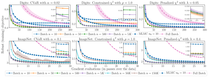
Figure 1: Convergence of DRO objective in our digits and ImageNet classification experiments. Shaded areas indicate range of variability across 5 repetitions (minimum to maximum), and the zoomed-in regions highlight the (often very low) “bias floor” of small batch sizes.

Discussion.

Our analysis in Section 3.1 bounds the suboptimality of solutions resulting from using a mini-batch estimators with batch size $n$, showing it must vanish as $n$ increases. Figure 1 shows that smaller batch sizes indeed converge to suboptimal solutions, and that their suboptimality becomes negligible very quickly: essentially every batch size larger than $10$ provides fairly small bias (with the exception of $\mathcal{L}_{\chi^{2}}$ in the digits experiment). The effect of bias is particularly weak for $\mathcal{L}_{\chi^{2}\textup{-pen}}$, consistent with its superior theoretical guarantees. We note, however, that the suboptimality we see in practice is far smaller than the worst-case bounds in Proposition 1. We investigate this in Appendix F.5, where we show that the bias $\mathcal{L}-\overline{\mathcal{L}}$ is in fact consistent with our theory, but the minimizers of $\mathcal{L}$ and $\overline{\mathcal{L}}$ are more similar than expected a priori.

While the MLMC estimator does not suffer from a bias floor (by design), it is also much slower to converge. This may appear confusing, since the MLMC convergence guarantees are optimal (for $\mathcal{L}_{\textup{CVaR}}$ and $\mathcal{L}_{\chi^{2}\textup{-pen}}$) while the mini-batch estimator achieves the optimal rate only under certain assumptions. Recall, however, that these assumptions are smoothness of the loss (which holds in our experiments) and—for CVaR—sufficiently rapid decay of the bias floor, which we verify empirically.

For batch sizes in the range 50–5K, the traces in Figure 1 look remarkably similar. This is consistent with our theoretical analysis for $\mathcal{L}_{\textup{CVaR}}$ and $\mathcal{L}_{\chi^{2}\textup{-pen}}$, which shows that the variance decreases linearly with the batch size and we may therefore (with Nesterov acceleration) increase the step size proportionally and expect the total work to remain constant. As theory predicts, this learning rate increase is only possible up to a certain batch size (roughly 5K in our experiments), after which larger batches become less efficient. Indeed, to reach within 2% of the optimal value, the full-batch method requires 27–36$\times$ more work than batch sizes 50–5K for ImageNet, and 9–16$\times$ more work for the digits experiment (see Table 5 and 6 for a precise breakdown of the number of epochs required per algorithm for each robust objective).

We also repeat our experiments with the dual SGM and prima-dual methods mentioned in Table 1 and compare them with them our proposed method; see Appendix F.6 for details.

We conclude the discussion by briefly touching upon the improvement that DRO yields in terms of generalization metrics; we provide additional detail in Appendix F.5. In digit recognition experiment we observe that, compared to ERM with tuned $\ell_{2}$ regularization, DRO enables strictly better tradeoff between average and worst-subgroup performance. Specifically, it provides significant improvements in the worst sub-group loss—between 17.5% and 27% compared to ERM—with no negligible degradation in average loss and accuracy. It also provides minor gains in worst-group accuracy. For ImageNet the effect is more modest: in the worst-performing 10 classes we observe improvements of 5–10% in log loss, as well as a roughly 4 point improvement in accuracy. These improvements, however, come at the cost of degradation in average performance: the average loss increases by up to 10% and the average accuracy drops by roughly 1 point.

Runtime comparison.

In Table 2 we report the gradient complexity and wallclock time to reach accuracy within 2% of the optimal value. For brevity, we show it for a single robust objective (penalized-$\chi^{2}$), but we observe that similar results across robust objectives. We note that for small batch sizes the time per epoch is significantly larger than for larger batch sizes, this due in part to parallelization in evaluating $\ell$ and $\nabla\ell$ and in part to logging and Python interpreter overhead, which increase linearly with the number of iterations. However, these effects diminish as the batch size grows, and for batch size 5K the wallclock time to reach an accurate solution is an order of magnitude smaller than with the full-batch method. We run our experiments with 4 Intel Xeon E5-2699 CPUs and 12–32Gb of memory. Increasing the number of CPUs or using GPUs would allow for greater parallelism and improve the runtime at greater batch sizes. However, increasing the model complexity (e.g., to a deep neural network) would have the opposite effect. Using 4 CPUs for linear classification gives roughly the same range of feasible batch sizes as a ResNet-50 on large GPU arrays.

		ImageNet times [minutes]			Digits times [minutes]
Algorithm		per epoch	to 2% of opt	# epochs	per epoch	to 2% of opt	# epochs
Batch	$n=10$	$120\pm 5$	$850\pm 30$	7	$0.80\pm 0.1$	$\infty$	$\infty$
	$n=50$	$23\pm 0.7$	$116\pm 4$	$\boldsymbol{5}$	$0.23\pm 0.01$	$24\pm 1$	$107\pm 1$
	$n=500$	$5.9\pm 0.2$	$29\pm 1$	$\boldsymbol{5}$	$0.056\pm 0.004$	$5.8\pm 0.4$	$\boldsymbol{104}\pm 1$
	$n=5K$	$3.3\pm 0.04$	$\boldsymbol{16.5}\pm 0.2$	$\boldsymbol{5}$	$0.033\pm 0.004$	$\boldsymbol{4.4}\pm 0.7$	$131\pm 6$
	$n=50K$	$2.2\pm 0.03$	$50\pm 0.9$	$22$	–	–	–
	$n=150K$	$2.1\pm 0.03$	$55\pm 0.7$	$26$	–	–	–
MLMC	$n_{0}=10$	$16\pm 1$	$\infty$	$\infty$	$0.34\pm 0.02$	$\infty$	$\infty$
Full-batch		$2.1$	$380$	$180$	$0.022$	$37.0$	$1680$

Table 2: Comparison wallclock time (in minutes) of the different algorithms, in terms of time per epoch and time to reach within 2% of the best training loss. In the last two columns, we report the number of epochs required to reach within 2% of the best training loss. We report $\infty$ for configurations that do not reach the sub-optimality goal for the duration of the experiment, and omit standard deviations when then they are $0$.

8 Conclusion

This work provides rigorous convergence guarantees for solving large-scale convex $\phi$-divergence DRO problems with stochastic gradient methods, laying out a foundation for their use in practice; we conclude it by highlighting two directions for further research.

First, while our work resolves the optimal theoretical convergence rates for CVaR and $\chi^{2}$ penalty objectives, the corresponding result for $\chi^{2}$ constraint remains open. In particular, there is a gap between our $O(\rho\epsilon^{-3})$ upper and the $\Omega(\rho\epsilon^{-2})$ lower bound of Duchi and Namkoong [18]. Moreover, combining the uniform convergence results in Duchi and Namkoong [18] with a cutting plane method gives complexity guarantees scaling a roughly as $\rho^{2}d^{2}\epsilon^{-2}$, so the $O(\rho\epsilon^{-3})$ rate can only be optimal in high-dimensional settings.

Second, understanding the practical benefit of large-scale $\phi$-divergence DRO for machine learning requires further research. Our experiments suggest that larger benefits are likely when (a) distinct subgroups are present in the data and (b) good calibration and hence low logarithmic loss (rather than simply high accuracy) is important. While our work focuses on convex losses $\ell$ for theoretical clarity and experimental simplicity, we note that all the algorithms we develop apply directly for non-convex losses. Furthermore, our bias and variance analyses are independent of the convexity of $\ell$, and our PyTorch implementation supports any prediction model via automatic differentiation. Therefore, a natural next step is to apply DRO for training modern predictors such as neural networks.

Acknowledgments

The authors would like to thank Hongseok Namkoong for discussions and insights, as well as Nimit Sohoni for comments on an earlier draft. DL, YC and JCD were supported by the NSF under CAREER Award CCF-1553086 and HDR 1934578 (the Stanford Data Science Collaboratory) and Office of Naval Research YIP Award N00014-19-2288. YC was supported by the Stanford Graduate Fellowship. AS is supported by a Microsoft Research Faculty Fellowship, NSF CAREER Award CCF-1844855, NSF Grant CCF-1955039, a PayPal research gift, and a Sloan Research Fellowship.

Appendix

Appendix A Extended preliminaries

In this section we collect several basic results which we use in subsequent derivations in the paper: Section A.1 gives several additional characterization of the robust objective $\mathcal{L}$, Section A.2 briefly discusses the computation of $\mathcal{L}$ and its costs, Section A.3 gives a short derivation of the complexity guarantees for “dual SGM” in Table 1, and Section A.4 introduces the notion of losses contained in a $\chi^{2}$ divergence ball. Finally, Section A.5 lists a few standard probabilistic bounds.

A.1 Characterization of the robust objective

Here we give several equivalent characterizations of the robust objective

$$\mathcal{L}(x;P)\coloneqq\sup_{Q\ll P:\mathrm{D}_{\phi}(Q,P)\leq\rho}\Big{\{}\operatorname{\mathbb{E}}_{S\sim Q}[\ell(x;S)]-\lambda\mathrm{D}_{\psi}(Q,P)\Big{\}}.$$ (18)

where $\psi$, $\phi$ are closed convex functions from $\mathbb{R}_{+}$ to $\mathbb{R}$ satisfying $\psi(1)=\phi(1)=0$,

$$\mathrm{D}_{\phi}(Q,P)\coloneqq\int\phi\left(\frac{\mathrm{d}Q}{\mathrm{d}P}\right)\mathrm{d}P,~{}~{}\mbox{and}~{}~{}\mathrm{D}_{\psi}(Q,P)\coloneqq\int\psi\left(\frac{\mathrm{d}Q}{\mathrm{d}P}\right)\mathrm{d}P.$$

For $\widehat{P}[s_{1}^{n}]$ uniform on $s_{1},s_{2},\ldots,s_{n}$ (which we abbreviate $s_{1}^{n}$), we write

$$\mathcal{L}(x;s_{1}^{n})\coloneqq\mathcal{L}(x;\widehat{P}[s_{1}^{n}])=\sup_{q\in\Delta^{n}:\sum_{i\leq n}\frac{1}{n}\phi(nq_{i})\leq\rho}\Bigg{\{}\sum_{i\leq n}\left(q_{i}\ell(x;s_{i})-\tfrac{1}{n}\psi(nq_{i})\right)\Bigg{\}}.$$ (19)

A.1.1 Inverse-cdf formulation

Instead of expressing the objective in terms of distribution over $\mathbb{S}$, we can characterize the robust loss in terms of the inverse cdf of the distribution (over $\mathbb{R}$) of $\ell(x;S)$. Let $F^{-1}$ denotes the inverse cdf of $\ell(x;S)$ under $P$. Note that $\ell(x;S)$ with $S\sim P$ is equal in distribution to $F^{-1}(U)$ with $U\sim\mathsf{Unif}([0,1])$. Therefore,

$$\mathcal{L}(x;P) \coloneqq\sup_{Q^{\prime}:\mathrm{D}_{\phi}(Q^{\prime},\mathsf{Unif}([0,1]))\leq\rho}\Big{\{}\operatorname{\mathbb{E}}_{U\sim Q^{\prime}}[F^{-1}(U)]-\lambda\mathrm{D}_{\psi}(Q^{\prime},\mathsf{Unif}([0,1]))\Big{\}}$$

$$=\sup_{r\in\mathcal{R}}\int_{0}^{1}\Big{[}r(u)F^{-1}(u)-\lambda\psi(r(u))\Big{]}\mathrm{d}u,$$ (20)

where the last equality follows from writing $r(u)=\frac{\mathrm{d}Q^{\prime}}{\mathrm{d}\mathsf{Unif}([0,1])}(u)$, and the set $\mathcal{R}$ is

$$\mathcal{R}\coloneqq\left\{r:[0,1]\to\mathbb{R}_{+}~{}\bigg{|}~{}\int_{0}^{1}r(u)\mathrm{d}u=1~{}~{}\mbox{and}~{}~{}\int_{0}^{1}\phi(r(u))\mathrm{d}u\leq\rho\right\}.$$ (21)

A.1.2 Dual formulation

We can convert the maximization over $r$ in Eq. (20) (or $Q$ in (18)) with minimization over Lagrange multipliers for the constraint that $r$ sums to 1 and the $\phi$-divergence constraint, yielding

$$\mathcal{L}(x;P) =\inf_{\eta\in\mathbb{R},\nu\geq 0}\Upsilon(x,\eta,\nu;P),~{}\mbox{where}~{}$$

$$\Upsilon(x,\eta,\nu;P)\coloneqq\int_{0}^{1}\sup_{r\in\mathbb{R}_{+}}\Big{[}rF^{-1}(u)-\eta(r-1)-\nu(\phi(r)-\rho)-\lambda\psi(r)\Big{]}\mathrm{d}u,$$ (22)

where the strong duality follows Shapiro [59, Sec. 3.2]. Writing $(g)^{*}[v]\coloneqq\sup_{t\in\mathrm{dom}(g)}\left\{vt-g(t)\right\}$ for the conjugate function of $g$, we may express $\Upsilon$ as

$$\Upsilon(x,\eta,\nu;P)=\int_{0}^{1}(\nu\phi+\lambda\psi)^{*}[F^{-1}(u)-\eta]\mathrm{d}u+\eta+\nu\rho=\operatorname{\mathbb{E}}(\nu\phi+\lambda\psi)^{*}[\ell(x;S)-\eta]+\eta+\nu\rho,$$ (23)

where the expectation is over $S\sim P$, i.e. the distribution from which we observe samples. On a finite sample $s_{1}^{n}$ we have

$$\Upsilon(x,\eta,\nu;s_{1}^{n})\coloneqq\Upsilon(x,\eta,\nu;\widehat{P}[s_{1}^{n}])=\frac{1}{n}\sum_{i\leq n}(\nu\phi+\lambda\psi)^{*}[\ell(x;s_{i})-\eta]+\eta+\nu\rho.$$

For pure-constraint objectives (with $\psi=0$), $\Upsilon$ simplifies to

$$\psi=0\implies\Upsilon(x,\eta,\nu;P)=\nu\operatorname{\mathbb{E}}_{S\sim P}\phi^{*}\left[\frac{\ell(x;S)-\eta}{\nu}\right]+\eta+\nu\rho.$$ (24)

For pure-penalty objective (with $\phi=0$) the Lagrange multiplier $\nu$ is unnecessary and we have

$$\phi=0\implies\Upsilon(x,\eta;P)=\lambda\operatorname{\mathbb{E}}_{S\sim P}\psi^{*}\left[\frac{\ell(x;S)-\eta}{\lambda}\right]+\eta.$$ (25)

Note that $\Upsilon$ is an expectation (i.e., an empirical risk) which means that to minimize $\mathcal{L}(x;P)$ we can, in principle, apply ERM jointly on $x,\eta$ and $\nu$, as we further discuss in Section A.3.

Finally, we note that any $Q^{\star}$ attaining the supremum in (18) is of the form

$$\frac{\mathrm{d}Q^{\star}}{\mathrm{d}P}(s)={(\nu^{\star}+\lambda\psi)^{*}}^{\prime}[\ell(x;s)-\eta^{\star}].$$

where $\eta^{\star}$ and $\nu^{\star}$ are optimal Lagrange multipliers in (22) and ${(\nu^{\star}+\lambda\psi)^{*}}^{\prime}$ is a subderivative of $(\nu^{\star}+\lambda\psi)^{*}$. For $\phi=0$ this specializes to

$$\frac{\mathrm{d}Q^{\star}}{\mathrm{d}P}(s)={\psi^{*}}^{\prime}\left[\frac{\ell(x;s)-\eta^{\star}}{\lambda}\right].$$

For a finite sample, we have

$$q^{\star}_{i}=\frac{1}{n}{\psi^{*}}^{\prime}\left[\frac{\ell(x;s_{i})-\eta^{\star}}{\lambda}\right].$$ (26)

A.1.3 Expressions for CVaR

Recall that CVaR at level $\alpha$ corresponds to $\phi=0$ and $\psi=\mathbb{I}_{[0,1/\alpha)}$. The dual expression of CVaR simplifies to [60, Example 6.16]

$$\mathcal{L}_{\textup{CVaR}}(x;P)=\inf_{\eta\in\mathbb{R}}\left\{\frac{1}{\alpha}\operatorname{\mathbb{E}}_{S\sim P}(\ell(x;S)-\eta)_{+}+\eta\right\}.$$

It also has a simple closed-form expression in terms of the inverse cdf of $\ell(x;S)$ [60, Theorem 6.2]:

$$\mathcal{L}_{\textup{CVaR}}(x;P)=\frac{1}{\alpha}\int_{1-\alpha}^{1}F^{-1}(u)\mathrm{d}u.$$ (27)

We note that this last expression is a direct consequence of (20), since $\mathcal{R}$ is the set of measures never exceeding $\frac{1}{\alpha}$. On a finite sample $s_{1}^{n}$ this gives the closed-form expression

$$\mathcal{L}_{\textup{CVaR}}(x;s_{1}^{n})=\frac{1}{\alpha n}\sum_{i=1}^{\lfloor\alpha n\rfloor}\ell(x;s_{(i)})+\left(1-\frac{\lfloor\alpha n\rfloor}{\alpha n}\right)\ell(x;s_{(\lfloor\alpha n\rfloor+1)}),$$ (28)

where $s_{(1)},\ldots,s_{(n)}$ are a permutation of $s_{1}^{n}$ satisfying $\ell(x;s_{(1)})\geq\ell(x;s_{(2)})\geq\cdots\geq\ell(x;s_{(n)})$. For $\alpha\leq 1/n$ we simply have $\mathcal{L}_{\textup{CVaR}}(x;s_{1}^{n})=\max_{i\leq n}\ell(x;s_{i})$.

The KL-divergence penalized CVaR at level $\alpha$ corresponds to $\psi(t)=\mathbb{I}_{[0,1/\alpha]}(t)+t\log t-t+1$, for which

$$\psi^{*}[v]=\begin{cases}e^{v}-1&v<\log\frac{1}{\alpha}\\ \frac{1}{\alpha}-1+\frac{1}{\alpha}(v-\log\frac{1}{\alpha})&\text{otherwise},\\ \end{cases}$$

and the dual expression for $\mathcal{L}_{\textup{kl-CVaR}}$ is given by (25). In the special case $\alpha\leq 1/n$ the CVaR constraint becomes inactive, and we can minimize over $\eta$ in closed form to obtain the standard “soft max” objective $\mathcal{L}_{\textup{kl-CVaR}}(x;s_{1}^{n})=\lambda\log\big{(}\frac{1}{n}\sum_{i\leq n}\exp\left(\ell(x;s_{i})/\lambda\right)\big{)}$.

A.1.4 Expressions for $\mathcal{L}_{\chi^{2}\textup{-pen}}$ and $\mathcal{L}_{\chi^{2}}$

The penalized version of the $\chi^{2}$ objective corresponds to $\phi(t)=0$ and $\psi(t)=\frac{1}{2}(t-1)^{2}$. Note that $\mathrm{D}_{\phi}(Q,P)$ is invariant under $\psi(t)\mapsto\psi(t)+c\cdot(t-1)$ for any $c\in\mathbb{R}$ because $\int(\frac{\mathrm{d}Q}{\mathrm{d}P}-1)\mathrm{d}P=0$. We find it more convenient to work with $\psi(t)=\frac{1}{2}(t-1)^{2}+(t-1)=\frac{1}{2}(t^{2}-1)$, for which the conjugate is simply $\psi^{*}[v]=\frac{1}{2}((v)^{2}_{+}+1)$. The dual form (25) gives

$$\mathcal{L}_{\chi^{2}\textup{-pen}}(x;P)=\inf_{\eta\in\mathbb{R}}\left\{\frac{1}{2\lambda}\operatorname{\mathbb{E}}_{S\sim P}{(\ell(x;S)-\eta)_{+}^{2}}+\frac{\lambda}{2}+\eta\right\}.$$ (29)

The infimum is attained at the $\eta^{\star}$ solving $\operatorname{\mathbb{E}}(\ell(x;S)-\eta^{\star})_{+}=\lambda$. In other words,

$$\eta^{\star}=\operatorname{\mathbb{E}}\left[\ell(x;S)\mid\ell(x;S)\geq\eta^{\star}\right]-\frac{\lambda}{\mathbb{P}(\ell(x;S)\geq\eta^{\star})}=\mathcal{L}_{\textup{CVaR}}^{F(\eta^{\star})}(x;P)-\frac{\lambda}{1-F(\eta^{\star})},$$

where $F(t)=\mathbb{P}(\ell(x;S)\leq t)$ is the cdf of $\ell(x;S)$. Letting $\mathfrak{G}(\eta^{\star})$ denote the event that $\ell(x;S)\geq\eta^{\star}$, substituting back to the expression for $\mathcal{L}_{\chi^{2}\textup{-pen}}$ gives

$$\mathcal{L}_{\chi^{2}\textup{-pen}}(x;P)=\operatorname{\mathbb{E}}\left[\ell(x;S)\mid\mathfrak{G}(\eta^{\star})\right]+\frac{1}{2\lambda}\mathrm{Var}\left[\ell(x;S)\mid\mathfrak{G}(\eta^{\star})\right]+\frac{\lambda}{2}\left(\frac{1}{\mathbb{P}(\mathfrak{G}(\eta^{\star}))}-1\right)^{2}.$$

In words, $\mathcal{L}_{\chi^{2}\textup{-pen}}$ is a sum of a CVaR (at level $F(\eta^{\star})$), a conditional variance regularization term and an outage probability regularization term. This expression simplifies considerably when $\lambda$ is sufficiently large. Specifically, we have,

$$\lambda\geq B \implies\lambda\geq\operatorname{\mathbb{E}}\ell(x;S)-F^{-1}(0)$$

$$\implies\eta^{\star}=\operatorname{\mathbb{E}}\ell(x;S)-\lambda~{}~{}\mbox{and}~{}~{}\mathbb{P}(\mathfrak{G}(\eta^{\star}))=1$$

$$\implies\mathcal{L}_{\chi^{2}\textup{-pen}}(x;P)=\operatorname{\mathbb{E}}\ell(x;S)+\frac{1}{2\lambda}\mathrm{Var}[\ell(x;S)].$$ (30)

That is, for sufficiently large $\lambda$ the objective $\mathcal{L}_{\chi^{2}\textup{-pen}}$ is simply the empirical risk with variance regularization (see also [18]).

For a finite sample we have

$$\mathcal{L}_{\chi^{2}\textup{-pen}}(x;s_{1}^{n})=\frac{1}{2\lambda n}\sum_{i\leq n}{(\ell(x;s_{i})-\eta^{\star}_{n})_{+}^{2}}+\frac{\lambda}{2}+\eta^{\star}_{n}.$$

Where $\eta^{\star}_{n}$ is the solution to $\sum_{i\leq n}{(\ell(x;s_{i})-\eta^{\star}_{n})_{+}}=n\lambda$, or equivalently

$$\eta^{\star}_{n}=\frac{1}{i^{\star}}\sum_{i\leq i^{\star}}\ell(x;s_{(i)})-\frac{\lambda n}{i^{\star}}~{}~{}\mbox{for the unique $i^{\star}$ such that}~{}~{}\ell(x;s_{(i^{\star}+1)})\leq\eta^{\star}_{n}\leq~{}\ell(x;s_{(i^{\star})}),$$ (31)

where $\{\ell(x;s_{(i)})\}$ are the sorted $\{\ell(x;s_{i})\}$ and $\ell(x;s_{(n+1)})\coloneqq-\infty$.

An expression for $\mathcal{L}_{\chi^{2}}$ follows via (29)

$$\mathcal{L}_{\chi^{2}}(x;P)=\inf_{\lambda\geq 0}\left\{\mathcal{L}_{\chi^{2}\textup{-pen}}(x;P)+\lambda\rho\right\}=\inf_{\eta\in\mathbb{R}}\left\{\sqrt{1+2\rho}\sqrt{\operatorname{\mathbb{E}}_{S\sim P}{(\ell(x;S)-\eta)_{+}^{2}}}+\eta\right\},$$ (32)

and the maximizing $Q$ is

$$\frac{\mathrm{d}Q^{\star}}{\mathrm{d}P}(s)=\frac{(\ell(x;s)-\eta^{\star})_{+}}{\operatorname{\mathbb{E}}_{S\sim P}(\ell(x;S)-\eta^{\star})_{+}}.$$ (33)

A.1.5 Expression for $\nabla\mathcal{L}$

Let $Q^{\star}$ by a distribution attaining the supremum in (18) and recall that $\nabla\ell(x;s)$ denotes an element in the sub-differential of $\ell(x;s)$ w.r.t. $x$. Then the following vector is a subgradient of $\mathcal{L}$ [33, Corollary 4.4.4],

$$\nabla\mathcal{L}(x;P)=\operatorname{\mathbb{E}}_{S\sim Q^{\star}}\nabla\ell(x;S).$$

Similarly, for a sample of size $n$ and a maximizing $q^{\star}$, we have

$$\nabla\mathcal{L}(x;s_{1}^{n})=\sum_{i\leq n}q^{\star}_{i}\nabla\ell(x;s_{i}).$$ (34)

A.1.6 Smoothness of $\mathcal{L}_{\chi^{2}\textup{-pen}}$ and $\mathcal{L}_{\textup{kl-CVaR}}$

The smoothness of $\mathcal{L}$ (i.e., Lipschitz continuity of its gradient) plays a role in our mini-batch gradient estimator complexity guarantees. When the penalty term $\psi$ is strongly convex, the maximizing $Q^{\star}$ (or $q^{\star}$) is unique, and if $\nabla\ell$ is $H$-Lipschitz then $\mathcal{L}$ is differentiable [33, Corollary 4.4.5]. In particular, writing $Q^{\star}_{x}$ for the maximizing $Q$ at point $x$, we have

$$\|\nabla\mathcal{L}(x;P)-\nabla\mathcal{L}(y;P)\|=\left\|\int\left\{\nabla\ell(x;s)\mathrm{d}Q^{\star}_{x}(y)-\nabla\ell(y;s)\mathrm{d}Q^{\star}_{y}(s)\right\}\right\|$$

$$\quad\quad\leq\int{\|\nabla\ell(x;s)-\nabla\ell(y;s)\|\mathrm{d}Q^{\star}_{x}(s)}+\int\|\nabla\ell(y;s)\|\left\lvert\frac{\mathrm{d}Q^{\star}_{x}}{\mathrm{d}P}(s)-\frac{\mathrm{d}Q^{\star}_{y}}{\mathrm{d}P}(s)\right\rvert\mathrm{d}P(s)$$

$$\quad\quad\leq H\|x-y\|+G\left\|Q^{\star}_{x}-Q^{\star}_{y}\right\|_{1}.$$ (35)

Therefore, if $Q^{\star}_{x}$ is Lipschitz w.r.t. $x$ in the 1-norm then $\nabla\mathcal{L}$ is Lipschitz as well. This is indeed the case $\mathcal{L}_{\chi^{2}\textup{-pen}}$ and $\mathcal{L}_{\textup{kl-CVaR}}$.

See 1

Proof.

Since entropy is 1-strongly-convex w.r.t. the 1-norm, for $\mathcal{L}_{\textup{kl-CVaR}}$ we have that the penalty $\lambda\psi$ is $\lambda$-strongly-convex w.r.t. the 1-norm and therefore [56, Lemma 2]

$$\left\|Q^{\star}_{x}-Q^{\star}_{y}\right\|_{1}\leq\frac{1}{\lambda}\|\ell(x;\cdot)-\ell(y;\cdot)\|_{\infty}\leq\frac{G}{\lambda}\|x-y\|,$$

which by (35) implies that $\nabla\mathcal{L}_{\textup{kl-CVaR}}$ is $(H+G^{2}/\lambda)$-Lipschitz as required. For $\mathcal{L}_{\chi^{2}\textup{-pen}}$, we find it easier to argue for a finite sample $s_{1}^{n}$. By (19) we have $q^{\star}_{x}=\operatorname*{arg\,max}_{q\in\Delta^{n}}\left\{q\top\ell(x)-\frac{1}{2}\lambda n\|q\|_{2}^{2}\right\}$, where $\ell_{i}(x)=\ell(x;s_{i})$. Therefore, by $\lambda n$ -strong-convexity w.r.t. the 2-norm, we have

$$\|q^{\star}_{x}-q^{\star}_{y}\|_{1}\leq\sqrt{n}\|q^{\star}_{x}-q^{\star}_{y}\|_{2}\leq\frac{1}{\lambda\sqrt{n}}\|\ell(x)-\ell(y)\|_{2}\leq\frac{G}{\lambda}\|x-y\|,$$

establishing that $\nabla\mathcal{L}_{\chi^{2}\textup{-pen}}$ is also $(H+G^{2}/\lambda)$-Lipschitz.

Finally, we note that $\mathcal{L}_{\textup{kl-CVaR}}(x;P)\leq\mathcal{L}_{\textup{CVaR}}$ because $D_{\psi}(Q,P)\geq 0$ for all $Q$. Conversely since any feasible $Q$ satisfies $\mathrm{d}Q/\mathrm{d}P\leq 1/\alpha$ we have $D_{\psi}(Q,P)=\int\mathrm{d}Q\log\frac{\mathrm{d}Q}{\mathrm{d}P}\leq\log\frac{1}{\alpha}$ and therefore $\mathcal{L}_{\textup{kl-CVaR}}(x;P)\geq\mathcal{L}_{\textup{CVaR}}(x;P)-\lambda\log\frac{1}{\alpha}$. ∎

A.2 Computational cost

To compute $\mathcal{L}(x;s_{1}^{n})$ and its (sub)gradient from $\{\ell(x;s_{i})\}_{i\leq n}$ and $\{\nabla\ell(x;s_{i})\}_{i\leq n}$ we compute $q^{\star}$ that maximizes (19) and substitute it back in (34). The substitution requires $O(nd)$ work, so it remains to account for the work in computing $q^{\star}$.

For CVaR, this clearly amounts to sorting $\{\ell(x;s_{i})\}_{i\leq n}$ and therefore takes $O(n\log n)$ time. Similarly, for $\mathcal{L}_{\chi^{2}\textup{-pen}}$ we may find sort the losses and find $i^{\star}$ in (31), and hence $\eta^{\star}_{n}$ and $q^{\star}$, in $O(n)$ time. Alternatively, for any objective with $\phi=0$ (including $\mathcal{L}_{\chi^{2}\textup{-pen}}$ and $\mathcal{L}_{\textup{kl-CVaR}}$ we can bisect directly on $\eta$, either to minimize the expression (25) or to satisfy the the simplex constraint $\sum_{i\leq n}q^{\star}_{i}=\frac{1}{n}\sum_{i\leq n}(\psi^{*})^{\prime}[(\ell(x;s_{i})-\eta^{\star})/\lambda]=1$.

For $\mathcal{L}_{\chi^{2}}$ we may find $q^{\star}$ by performing similar bisection over $\eta$ via the expression (32), again either minimizing it or solving for the condition $\frac{1}{n}\sum_{i\leq n}(\ell(x;s_{i})-\eta^{\star})_{+}^{2}=(1+2\rho)\big{(}\frac{1}{n}\sum_{i\leq n}(\ell(x;s_{i})-\eta^{\star})_{+}\big{)}^{2}$. Finding an $\varepsilon$ accurate solution via bisection requires roughly $n\log\frac{B}{\varepsilon}$ time.

Since we are interested in large-scale application, we assume that $d\gg\log(nB/\varepsilon)$ and therefore the time to compute the objective and its gradient is $O(nd)$.

For simplicity and stability, our code implements the computation of $q^{\star}$ using bisection over $\eta$ for each of $\mathcal{L}_{\chi^{2}\textup{-pen}},\mathcal{L}_{\chi^{2}}$ and $\mathcal{L}_{\textup{kl-CVaR}}$.

A.3 Stochastic gradient method on the dual objective

Here we discuss the convergence guarantees for a simple stochastic gradient method using the dual expression (22) for $\mathcal{L}(x;P_{0})$ in order to minimize it over $x$. While several works consider such methods (see Section 1.1), we could not find direct reference for their runtime guarantees, and we therefore briefly derive it below.

Focusing on objectives with $\phi=0$ (as in (25)), and writing $\gamma_{x}$ and $\gamma_{\eta}$ for step sizes, we write the iterations on $x$ and the Lagrange multiplier $\eta$ as

$$x_{t+1} =\Pi_{\mathcal{X}}\left(x_{t}-\gamma_{x}\nabla\Upsilon(x_{t},\eta_{t};P_{0})\right)=\Pi_{\mathcal{X}}\left(x_{t}-\gamma_{x}{\psi^{*}}^{\prime}\left[\frac{\ell(x;S_{i})-\eta_{t}}{\lambda}\right]\nabla\ell(x;S_{i})\right),~{}~{}\mbox{and}$$

$$\eta_{t+1} =\Pi_{[\underline{\eta},\overline{\eta}]}\left(\eta_{t}-\gamma_{\eta}\frac{\partial}{\partial\eta}\Upsilon(x_{t},\eta_{t};P_{0})\right)=\Pi_{[\underline{\eta},\overline{\eta}]}\left(\eta_{t}+\gamma_{\eta}{\psi^{*}}^{\prime}\left[\frac{\ell(x;S_{i})-\eta_{t}}{\lambda}\right]-\gamma_{\eta}\right),$$ (36)

Where $S_{1},S_{2},\ldots$ are drawn iid from $P_{0}$.

For CVaR, we have $(\psi^{*})^{\prime}[v]=\frac{1}{\alpha}1_{\{v\geq 0\}}$ and we may restrict $\eta$ to the range $[\underline{\eta},\overline{\eta}]=[0,B]$, as the optimal $\eta$ is the value at risk level $\alpha$ and therefore in the range of $\ell$. For $\mathcal{L}_{\chi^{2}\textup{-pen}}$ we have $(\psi^{*})^{\prime}[v]=(v)_{+}$ and we may take $[\underline{\eta},\overline{\eta}]=[-\lambda,B]$ due to the condition $\operatorname{\mathbb{E}}(\ell(x;S)-\eta^{\star})_{+}=\lambda$. In these settings, the method (36) has the following guarantee

Claim 3.

Let $\epsilon\in(0,B)$. For CVaR and a suitable choice of $\gamma_{x},\gamma_{\eta}$ the average iterate $\bar{x}_{T}=\frac{1}{T}\sum_{t\leq T}x_{t}$ satisfies

$$\operatorname{\mathbb{E}}\mathcal{L}_{\textup{CVaR}}(\bar{x}_{T};P_{0})-\min_{x^{\prime}\in\mathcal{X}}\mathcal{L}_{\textup{CVaR}}(x^{\prime};P_{0})\leq\epsilon~{}~{}\mbox{for}~{}~{}T\asymp\frac{(GR)^{2}+B^{2}}{\alpha^{2}\epsilon^{2}}.$$

Similarly, for $\chi^{2}$ penalty we have

$$\operatorname{\mathbb{E}}\mathcal{L}_{\chi^{2}\textup{-pen}}(\bar{x}_{T};P_{0})-\min_{x^{\prime}\in\mathcal{X}}\mathcal{L}_{\chi^{2}\textup{-pen}}(x^{\prime};P_{0})\leq\epsilon~{}~{}\mbox{for}~{}~{}T\asymp\frac{(GR)^{2}+B^{2}}{\epsilon^{2}}\left(1+\frac{B^{2}}{\lambda^{2}}\right).$$

Proof.

By Proposition 3, the expected sub-optimality of $\bar{x}_{T}$ is $\lesssim(\Gamma_{x}R+\Gamma_{\eta}(\overline{\eta}-\underline{\eta})/\sqrt{T}$, where $\Gamma_{x}^{2}$ (respectively $\Gamma_{\eta}$) is an upper bound on the second moment of $\nabla\Upsilon(x,\eta;S)$ (respectively $\frac{\partial}{\partial\eta}\Upsilon(x,\eta;S)$). For $\mathcal{L}_{\textup{CVaR}}$ we have $\Gamma_{x}\leq G/\alpha$, $\Gamma_{\eta}\leq 1/\alpha$ and $\overline{\eta}-\underline{\eta}=B$. For $\mathcal{L}_{\chi^{2}\textup{-pen}}$ we have $\Gamma_{x}\leq G(1+B/\lambda)$, $\Gamma_{\eta}=1+B/\lambda$ and $\overline{\eta}-\underline{\eta}=B+\lambda$. The result follows from substituting $T\asymp\left(\Gamma_{x}^{2}R^{2}+\Gamma_{\eta}^{2}(\overline{\eta}-\underline{\eta})^{2}\right)\epsilon^{-2}$. ∎

A.4 Uncertainty sets contained in $\chi^{2}$ divergence balls

A number of our results hold for general subclass of the objective (18) with the following property.

Definition 1 ($\chi^{2}$-bounded objective).

An objective $\mathcal{L}(x;P_{0})$ is $C$-$\chi^{2}$-bounded if for all $x$ and all $Q^{\star}$ attaining the supremum in (18) we have $\mathrm{D}_{\chi^{2}}(Q^{\star},P_{0})\leq C$.

The three objectives we focus on are $\chi^{2}$-bounded.

Claim 4.

The objectives $\mathcal{L}_{\textup{kl-CVaR}},\mathcal{L}_{\chi^{2}}$ and $\mathcal{L}_{\chi^{2}\textup{-pen}}$ are $\chi^{2}$-bounded with constants $C=\frac{1}{\alpha}-1$, $C=\rho$ and $C=B/\lambda$, respectively.

Proof.

That $\mathcal{L}_{\chi^{2}}$ is $\rho$-$\chi^{2}$-bounded is obvious from definition. For $\mathcal{L}_{\chi^{2}\textup{-pen}}$ we have

$$\mathcal{L}_{\chi^{2}\textup{-pen}}(x;P_{0}) =\operatorname{\mathbb{E}}_{S\sim Q^{\star}}\ell(x;S)-\lambda\mathrm{D}_{\chi^{2}}(Q^{\star},P_{0})$$

$$\geq\operatorname{\mathbb{E}}_{S\sim P_{0}}\ell(x;S)-\lambda\mathrm{D}_{\chi^{2}}(P_{0};P_{0})=\operatorname{\mathbb{E}}_{S\sim P_{0}}\ell(x;S)$$

and consequently

$$\mathrm{D}_{\chi^{2}}(Q^{\star},P_{0})\leq\frac{E_{S\sim Q^{\star}}\ell(x;S)-\operatorname{\mathbb{E}}_{S\sim P_{0}}\ell(x;S)}{\lambda}\leq\frac{B}{\lambda}.$$

Finally, for $\mathcal{L}_{\textup{kl-CVaR}}$ every feasible $Q$ satisfies $\mathrm{d}Q/\mathrm{d}P_{0}\leq 1/\alpha$ and therefore

$$\mathrm{D}_{\chi^{2}}(Q,P_{0})=\int\left(\frac{\mathrm{d}Q}{\mathrm{d}P_{0}}(s)\right)^{2}\mathrm{d}P_{0}(s)-1\leq\frac{1}{\alpha}\left(\frac{\mathrm{d}Q}{\mathrm{d}P_{0}}(s)\right)\mathrm{d}P_{0}(s)-1=\frac{1}{\alpha}-1.$$

∎

A.5 General results

We conclude this section of the appendix by stating three general results that aid our analysis. First, we give a lemma stating that a binomial random variable with parameters $n$ and $\alpha$ has a constant probability of being at least $\sqrt{\alpha(1-\alpha)n}$ below its mean.

Lemma 4.

Let $n\in\mathbb{N}$ and $\alpha\in(0,1)$. There exists a numerical constant $C\in\mathbb{R}$ such that

$$\mathbb{P}\big{(}\mathsf{Bin}(n,\alpha)\leq n\alpha-\sqrt{n\alpha(1-\alpha)}\big{)}\geq\mathbb{P}(\mathcal{N}(0,1)\leq-1)-\frac{C}{\sqrt{\alpha(1-\alpha)n}}.$$

Proof.

Note that $\mathbb{P}\big{(}\mathsf{Bin}(n,\alpha)\leq n\alpha-\sqrt{n\alpha(1-\alpha)}\big{)}=\mathbb{P}(Y\sqrt{n}\leq-1)$ where $Y=\frac{1}{n}\frac{\mathsf{Bin}(n,\alpha)-n\alpha}{\sqrt{\alpha(1-\alpha)}}$ is the mean of $n$ independent random variable with zero mean, unit variance, and absolute third moment $\rho=\frac{\alpha^{2}+(1-\alpha)^{2}}{\sqrt{\alpha(1-\alpha)}}\leq\frac{1}{\sqrt{\alpha(1-\alpha)}}$. The Berry-Esseen theorem [21, Theorem 3.4.17] states that for such $Y$ we have $|\mathbb{P}(Y\sqrt{n}\leq t)-\mathbb{P}(\mathcal{N}(0,1)\leq t)|\leq C\rho/\sqrt{n}$, for all $t\in\mathbb{R}$; substituting $t=1$ and $\rho\leq\frac{1}{\sqrt{\alpha(1-\alpha)}}$ concludes the proof. ∎

Second, we state the Efron-Stein inequality in vector form, which follows from applying the standard scalar bound element-wise.

Lemma 5 (Efron-Stein inequality [8, Theorem 3.1]).

Let $X_{1}^{n+1}$ be i.i.d random variables and $f:\mathcal{X}^{n}\to\mathbb{R}^{m}$. Let $I$ be uniform on $\{1,\ldots,n\}$ and let $\tilde{X}_{1}^{N}$ be such that $\tilde{X}_{i}=X_{i}$ for $i\neq I$ and $\tilde{X}_{I}=X_{n+1}$. Then

$$\mathrm{Var}[f(X_{1}^{n})]\leq\frac{n}{2}\operatorname{\mathbb{E}}{}\|f(X_{1}^{n})-f(\tilde{X}_{1}^{n})\|^{2}.$$ (37)

Third, we give a general lemma on the variance of sampling without replacement, which we specialize to the simplex for later use.

Lemma 6.

Let $p\in\Delta^{k}$ and let $\mathcal{I}$ be a random subset of $[k]$ of size $k/2$. Then

$$\operatorname{\mathbb{E}}\Bigg{(}\sum_{i\in\mathcal{I}}p_{i}-\frac{1}{2}\Bigg{)}^{2}\leq\frac{1}{2}\Big{\|}p-\tfrac{1}{k}\boldsymbol{1}\Big{\|}^{2}=\frac{1}{2k}\mathrm{D}_{\chi^{2}}(p,\tfrac{1}{k}\boldsymbol{1}).$$

Proof.

Let us denote $q=p-\tfrac{1}{k}\boldsymbol{1}$. We have

$$\operatorname{\mathbb{E}}\left(\sum_{i\leq k}p_{i}1_{\{i\in\mathcal{I}\}}-\frac{1}{2}\right)^{2} =\operatorname{\mathbb{E}}\left(\sum_{i\leq k}q_{i}1_{\{i\in\mathcal{I}\}}\right)^{2}$$

$$\stackrel{{\scriptstyle(i)}}{{=}}\frac{1}{2}\sum_{i\leq k}q_{i}^{2}+\sum_{i\neq j}q_{i}q_{j}\operatorname{\mathbb{E}}1_{\{i\in\mathcal{I}\mbox{~{}and~{}}j\in\mathcal{I}\}}$$

$$\stackrel{{\scriptstyle(ii)}}{{=}}\frac{1}{2}\|q\|^{2}+\frac{k-2}{4(k-1)}\sum_{i\leq k}\sum_{j\neq i}q_{i}q_{j}=\frac{1}{2}\|q\|^{2}+\frac{k-2}{4(k-1)}\sum_{i\leq k}q_{i}(1-q_{i})$$

$$\stackrel{{\scriptstyle(iii)}}{{=}}\left(\frac{1}{2}-\frac{k-2}{4(k-1)}\right)\|q\|^{2}\leq\frac{1}{2}\|q\|^{2},$$

where $(i)$ stems from $\mathbb{P}(i\in\mathcal{I})=\frac{1}{2}$, $(ii)$ from $\mathbb{P}(i\in I\mbox{~{}and~{}}j\in I)=\frac{1}{2}\frac{k/2-1}{k-1}$ and $(iii)$ from $\sum_{i\leq k}q_{i}=0$. Noting that $\mathrm{D}_{\chi^{2}}(p,\tfrac{1}{k}\boldsymbol{1})=k\|q\|^{2}$ concludes the proof. ∎

Appendix B Proofs from Section 3

This section completes the proof and discussion of the results in Section 3. First, in Section B.1, we prove the bias bounds in Proposition 1 and argue their tightness in the worst case. Section B.2 provides additional discussion of the smoothness and Lipschitz inverse-cdf assumptions sometimes used in this section. Then, in Section B.3 we bound the variance of the mini-batch estimators for $\chi^{2}$-bounded penalty objectives and their gradient, obtaining Proposition 2 as a corollary. We also argue that similar bounds do not hold for the $\chi^{2}$ constraint objective. In Section B.4 we review the standard convergence guarantees for stochastic gradients iterations with and without Nesterov acceleration, and in Section B.5 we combine all these ingredients to prove Theorem 1.

B.1 Bias of batch estimator

B.1.1 Proof of Proposition 1

See 1

Proof.

We first show that the bound $\mathcal{L}\geq\overline{\mathcal{L}}$ holds for any loss of the form (18) and then proceed to show each of the bounds (8)–(11). We remark here that the bound (9) actually holds for any $\rho$-$\chi^{2}$-bounded objective (Definition 1).

Proof of $\mathcal{L}(x;P_{0})\geq\overline{\mathcal{L}}(x;n)$.

The dual expression (23) gives

$$\mathcal{L}(x;P_{0}) =\inf_{\eta\in\mathbb{R},\nu\geq 0}\operatorname{\mathbb{E}}_{S\sim P_{0}}\left\{(\nu\phi+\lambda\psi)^{*}[\ell(x;S)-\eta]+\eta+\nu\rho\right\}$$

$$=\inf_{\eta\in\mathbb{R},\nu\geq 0}\operatorname{\mathbb{E}}_{S_{1}^{n}\sim P_{0}^{n}}\Bigg{\{}\frac{1}{n}\sum_{i\leq n}(\nu\phi+\lambda\psi)^{*}[\ell(x;S_{i})-\eta]+\eta+\nu\rho\Bigg{\}}$$

$$\geq\operatorname{\mathbb{E}}_{S_{1}^{n}\sim P_{0}^{n}}\inf_{\eta\in\mathbb{R},\nu\geq 0}\Bigg{\{}\frac{1}{n}\sum_{i\leq n}(\nu\phi+\lambda\psi)^{*}[\ell(x;S_{i})-\eta]+\eta+\nu\rho\Bigg{\}}=\operatorname{\mathbb{E}}\mathcal{L}(x;S_{1}^{n})=\overline{\mathcal{L}}(x;n),$$

where the inequality follows from exchanging the expectation and the infimum.

Proof of the CVaR bias bound (8).

By Eq. (28) we have

$$\overline{\mathcal{L}}_{\textup{CVaR}}(x;n)=\operatorname{\mathbb{E}}\mathcal{L}_{\textup{CVaR}}(x;S_{1}^{n})=\frac{1}{\alpha n}\sum_{i=1}^{\lfloor\alpha n\rfloor}\operatorname{\mathbb{E}}\ell(x;S_{(i)})+\left(1-\frac{\lfloor\alpha n\rfloor}{\alpha n}\right)\operatorname{\mathbb{E}}\ell(x;S_{(\lfloor\alpha n\rfloor+1)}),$$

where $\ell(x;S_{(i)})$ is the $i$th order statistic of $\ell(x;S_{1}^{n})$ (in decreasing order). Recalling that $F$ denotes the cdf of $\ell(x;S)$, we may write $\ell(x;S)=F^{-1}(U)$ with $U$ uniform on $[0,1]$. Therefore, $\ell(x;S_{(i)})=F^{-1}(U_{(i)})$ where $U_{(i)}\sim\mathsf{Beta}(n-i+1,i)$ is the $i$th order statistic of $n$ iid $\mathsf{Unif}([0,1])$ random variables [50, Sec. 4.6]. Taking expectation, we have

$$\operatorname{\mathbb{E}}_{S_{1}^{n}\sim P_{0}^{n}}\ell(x;S_{(i)})=\int_{0}^{1}F_{Z}^{-1}(u)f_{\mathsf{Beta}(n-i+1,i)}(u)\mathrm{d}u,$$

where $f_{\mathsf{Beta}(a,b)}$ is the density function of the Beta random variable of parameters $a,b$. Substituting back, we have

$$\overline{\mathcal{L}}_{\textup{CVaR}}(x;n) =\frac{1}{\alpha}\int_{0}^{1}\mathcal{I}_{\alpha}(u)F^{-1}(u)\mathrm{d}u,~{}~{}\mbox{where}~{}~{}$$

$$\mathcal{I}_{\alpha}(u)=\frac{1}{n}\sum_{i=1}^{\lfloor\alpha n\rfloor}f_{\mathsf{Beta}(n-i+1,i)}(u)+\left(\alpha-\frac{\lfloor\alpha n\rfloor}{n}\right)f_{\mathsf{Beta}(n-\lfloor\alpha n\rfloor,\lfloor\alpha n\rfloor+1)}(u).$$ (38)

Using

$$\begin{split}\frac{1}{n}\sum_{i=1}^{n}f_{\mathsf{Beta}(n-i+1,i)}(u)&=\frac{1}{n}\sum_{i=1}^{n}\frac{n!}{(n-i)!(i-1)!}u^{n-i}(1-u)^{i-1}\\ &=\sum_{i=0}^{n-1}{n-1\choose i-1}(1-u)^{i}u^{n-1-i}=1,\end{split}$$ (39)

we have that

$$1-\mathcal{I}_{\alpha}(u)\leq\frac{1}{n}\sum_{i=\lfloor\alpha n\rfloor+1}^{n}f_{\mathsf{Beta}(n-i+1,i)}(u).$$

Recalling Eq. (27) for $\mathcal{L}_{\textup{CVaR}}(x;P_{0})$, and recalling that $F^{-1}(u)\in[0,B]$ for all $u$ by assumption, we bound the bias as

$$\mathcal{L}_{\textup{CVaR}}(x;P_{0})-\overline{\mathcal{L}}_{\textup{CVaR}}(x;n) =\frac{1}{\alpha}\int_{0}^{1}\left[1_{\{u\geq 1-\alpha\}}-\mathcal{I}_{\alpha}(u)\right]F^{-1}(u)\mathrm{d}u$$

$$\leq\frac{B}{\alpha}\int_{1-\alpha}^{1}\left[1_{\{u\geq 1-\alpha\}}-\mathcal{I}_{\alpha}(u)\right]\mathrm{d}u$$

$$\leq\frac{B}{\alpha}\int_{1-\alpha}^{1}\left(\frac{1}{n}\sum_{i=\lfloor\alpha n\rfloor+1}^{n}f_{\mathsf{Beta}(n-i+1,i)}(u)\right)\mathrm{d}u$$

$$=\frac{B}{\alpha n}\sum_{i=\lfloor\alpha n\rfloor+1}^{n}\mathbb{P}(\mathsf{Beta}(n-i+1,i)\geq 1-\alpha).$$ (40)

To conclude, it suffices to bound the tail probability of the Beta random variables. We have [see, e.g., 50, Ex. 5 in Sec. 4.6]

$$\mathbb{P}(\mathsf{Beta}(n-i+1,i)\geq 1-\alpha) =1-\mathbb{P}(\mathsf{Beta}(n-i+1,i)\leq 1-\alpha)$$

$$=\mathbb{P}(\mathsf{Bin}(n;1-\alpha)\leq n-i)=\mathbb{P}(\mathsf{Bin}(n;\alpha)\geq i),$$

and the multiplicative Chernoff bound [40, Theorem 4.3] gives

$$\mathbb{P}(\mathsf{Bin}(n;\alpha)\geq i)\leq\exp\left(-\frac{i-n\alpha}{3}\min\left\{\frac{i-n\alpha}{n\alpha},1\right\}\right).$$

Therefore, for $\alpha n\geq 9$,

$$\sum_{i=\lfloor\alpha n\rfloor+1}^{n}\mathbb{P}(\mathsf{Bin}(n;\alpha)\geq i) \leq\sum_{i=\lfloor\alpha n\rfloor+1}^{2\lfloor\alpha n\rfloor}\exp\left(-\frac{(i-n\alpha)^{2}}{3n\alpha}\right)+\sum_{i=2\lfloor\alpha n\rfloor+1}^{\infty}\exp\left(-\frac{i-n\alpha}{3}\right)$$

$$\leq 1+\int_{0}^{\infty}\exp\left(-\frac{u^{2}}{3n\alpha}\right)\mathrm{d}u+\exp\left(-\frac{2\lfloor\alpha n\rfloor+1-\alpha n}{3}\right)\sum_{i=0}^{\infty}e^{-i/3}$$

$$\leq 1+\frac{\sqrt{3\pi\alpha n}}{2}+\frac{e^{-3}}{1-e^{-1/3}}\leq 3\sqrt{\alpha n}.$$

Substituting into (40) and using $\mathcal{L}_{\textup{CVaR}}(x;P_{0})\leq B$ when $\alpha n\leq 9$ gives the final bound

$$\mathcal{L}_{\textup{CVaR}}(x;P_{0})-\overline{\mathcal{L}}_{\textup{CVaR}}(x;n)\leq B\min\left\{\frac{3}{\sqrt{\alpha n}},1\right\}.$$ (41)

Proof of the bound (9).

We start with the expression (20) specialized for the $\mathcal{L}_{\chi^{2}}$,

$$\mathcal{L}_{\chi^{2}}(x;P_{0})=\sup_{r\in\mathcal{R}}\int_{0}^{1}r(\beta)F^{-1}(1-\beta)\mathrm{d}\beta,$$

where

$$\mathcal{R}=\left\{r:[0,1]\to\mathbb{R}_{+}~{}\Big{|}~{}\|r\|_{1}=1,~{}\|r\|_{2}^{2}\leq 1+2\rho,~{}\mbox{and $r$ is non-increasing}\right\};$$

The restriction of $\mathcal{R}$ to non-increasing functions is “free” since $F^{-1}$ is non-decreasing. Our strategy is to relate $F^{-1}$ to CVaR and then apply the corresponding bias bounds (8)—this type of transformation is closely related to the Kusuoka representation of coherent risk measures [37]. Specifically, note that

$$\mathcal{L}_{\textup{CVaR}}^{\alpha}=\frac{1}{\alpha}\int_{0}^{\alpha}F^{-1}_{Z}(1-\beta)\mathrm{d}\beta\implies F^{-1}_{Z}(1-\alpha)=\frac{\mathrm{d}}{\mathrm{d}\alpha}(\alpha\mathcal{L}_{\textup{CVaR}}^{\alpha}).$$

Therefore, for any $r\in\mathcal{R}$ integration by parts gives

$$\int_{0}^{1}r(\beta)F_{Z}^{-1}(1-\beta)\mathrm{d}\beta=\int_{0}^{1}r(\alpha)\frac{\mathrm{d}}{\mathrm{d}\alpha}(\alpha\mathcal{L}_{\textup{CVaR}}^{\alpha})\mathrm{d}\alpha=r(1)\mathcal{L}_{\textup{CVaR}}^{1}-\int_{0}^{1}r^{\prime}(\alpha)\alpha\mathcal{L}_{\textup{CVaR}}^{\alpha}d\alpha.$$

The CVaR bias bound (41) tells us that $\mathcal{L}_{\textup{CVaR}}^{\alpha}\leq\overline{\mathcal{L}}_{\textup{CVaR}}^{\alpha}+\mathrm{bb}(\alpha)$ where $\mathrm{bb}(\alpha)=3B\min\left\{\sqrt{\frac{1}{\alpha n}},1\right\}$. Moreover, we may write $\overline{\mathcal{L}}_{\textup{CVaR}}^{\alpha}=\frac{1}{\alpha}\int_{0}^{\alpha}\operatorname{\mathbb{E}}\widehat{F}^{-1}(1-\beta)\mathrm{d}\beta$, where $\widehat{F}$ denotes the empirical cdf of the losses $\ell(x;S_{1}),\ldots,\ell(x;S_{n})$. Noting that $r^{\prime}(\alpha)\leq 0$ for all $\alpha$, we may write

$$-\int_{0}^{1}r^{\prime}(\alpha)\alpha\mathcal{L}_{\textup{CVaR}}^{\alpha}d\alpha \leq-\int_{0}^{1}r^{\prime}(\alpha)\alpha\overline{\mathcal{L}}_{\textup{CVaR}}^{\alpha}d\alpha-\int_{0}^{1}r^{\prime}(\alpha)\alpha\cdot\mathrm{bb}(\alpha)d\alpha$$

$$=\operatorname{\mathbb{E}}\int_{0}^{1}r(\beta)\widehat{F}^{-1}(1-\beta)\mathrm{d}\beta-r(1)\overline{\mathcal{L}}_{\textup{CVaR}}^{1}+\int_{0}^{1}[r(\alpha)-r(1)](\alpha\cdot\mathrm{bb}(\alpha))^{\prime}\mathrm{d}\alpha,$$

where in the final equality we used again integration by parts along with $\operatorname{\mathbb{E}}\widehat{F}^{-1}(1-\alpha)=\frac{\mathrm{d}}{\mathrm{d}\alpha}(\alpha\overline{\mathcal{L}}_{\textup{CVaR}})$.

Substituting back and using $\mathcal{L}_{\textup{CVaR}}^{1}=\overline{\mathcal{L}}_{\textup{CVaR}}^{1}=\operatorname{\mathbb{E}}\ell(x;S)$, we obtain

$$\int_{0}^{1}r(\beta)F_{Z}^{-1}(1-\beta)\mathrm{d}\beta-\operatorname{\mathbb{E}}\int_{0}^{1}r(\beta)\widehat{F}^{-1}(1-\beta)\mathrm{d}\beta\leq\sup_{r\in\mathcal{R}}\int_{0}^{1}[r(\alpha)-r(1)](\alpha\cdot\mathrm{bb}(\alpha))^{\prime}\mathrm{d}\alpha\eqqcolon E$$

Taking a supremum over $r\in\mathcal{R}$, we conclude that

$$\mathcal{L}_{\chi^{2}}(x;P_{0}) =\sup_{r\in\mathcal{R}}\int_{0}^{1}r(\beta)F_{Z}^{-1}(1-\beta)\mathrm{d}\beta\leq\sup_{r\in\mathcal{R}}\operatorname{\mathbb{E}}\int_{0}^{1}r(\beta)\widehat{F}^{-1}(1-\beta)\mathrm{d}\beta+E$$

$$\leq\operatorname{\mathbb{E}}\sup_{r\in\mathcal{R}}\int_{0}^{1}r(\beta)\widehat{F}^{-1}(1-\beta)\mathrm{d}\beta+E=\overline{\mathcal{L}}_{\chi^{2}}(x;n)+E.$$ (42)

It remains to bound the quantity $E$, which we do via the the Cauchy-Schwarz inequality and the definition of $\mathcal{R}$, which gives

$$E=\int_{0}^{1}[r(\alpha)-r(1)](\alpha\cdot\mathrm{bb}(\alpha))^{\prime}\mathrm{d}\alpha\leq\|r\|_{2}\|(\alpha\cdot\mathrm{bb}(\alpha)^{\prime}\|_{2}\leq\sqrt{1+2\rho}\cdot\|(\alpha\cdot\mathrm{bb}(\alpha))^{\prime}\|_{2}$$

for all $r\in\mathcal{R}$. We calculate $(\alpha\cdot\mathrm{bb}(\alpha))^{\prime}=\mathrm{bb}(0)1_{\{\alpha\leq 1/n\}}+\frac{1}{2}\mathrm{bb}(\alpha)1_{\{\alpha>1/n\}}$, so that

$$\|(\alpha\cdot\mathrm{bb}(\alpha)^{\prime}\|_{2}^{2}=\frac{\mathrm{bb}^{2}(0)}{n}\left(1+\int_{1/n}^{1}\frac{\mathrm{d}\beta}{4\beta}\right)\leq(3B)^{2}\cdot\frac{4+\log n}{4n}.$$

for all $r\in\mathcal{R}$, giving the required bound.

Remark 1.

The bound (42) hold for any loss (18) and not just $\mathcal{L}_{\chi^{2}}$. Moreover, the final bound using Cauchy-Schwarz is equally valid for any $\rho$-$\chi^{2}$-bounded uncertainty set. In particular, consider the Cressie-Read uncertainty sets [12] corresponding to $k$-norm the constraint $\|r\|_{k}^{2}\leq 1+2\rho$. For $k>2$ they satisfy $\|r\|_{2}^{2}\leq 1+2\rho$ and our bias bounds holds (using Hölder’s inequality instead of Cauchy-Schwarz removes the logarithmic factor). For $k\in(1,2)$ Hölder’s inequality gives bounds decaying as $n^{-(k-1)/k}$.

Proof of the bound (11)

Starting with CVaR, we return to the expression (38) for the bias and note that

$$\left[1_{\{u\geq 1-\alpha\}}-\mathcal{I}_{\alpha}(u)\right]F^{-1}(u)\leq\left[1_{\{u\geq 1-\alpha\}}-\mathcal{I}_{\alpha}(u)\right]\left\{F^{-1}(1-\alpha)+G_{\textup{icdf}}\cdot(u-(1-\alpha))\right\}$$

holds for all $u$, because when $u<1-\alpha$ we have that $1_{\{u\geq 1-\alpha\}}-\mathcal{I}_{\alpha}(u)\leq 0$ and so we increase the LHS by replacing $F^{-1}$ with an under-estimate, while for $u\geq 1-\alpha$ we have $1-\mathcal{I}_{\alpha}(u)\geq 0$ due to (39) and we increase the LHS be replacing it with an $F^{-1}$ with an over-estimate. Substituting into (38) and calculating gives

$$\mathcal{L}_{\textup{CVaR}}(x;P_{0})-\overline{\mathcal{L}}_{\textup{CVaR}}(x;n)$$

$$\quad\leq\frac{1}{\alpha}\int_{0}^{1}\left(1_{\{u\geq 1-\alpha\}}-\mathcal{I}_{\alpha}\left(u\right)\right)\left[F^{-1}\left(1-\alpha\right)+G_{\textup{icdf}}\cdot\left(u-\left[1-\alpha\right]\right)\right]\mathrm{d}u$$

$$\quad\overset{\left(i\right)}{=}\frac{G_{\textup{icdf}}}{\alpha}\int_{0}^{1}\left(1_{\{u\geq 1-\alpha\}}-\mathcal{I}_{\alpha}\left(u\right)\right)u\mathrm{d}u$$

$$\quad\overset{\left(ii\right)}{=}G_{\textup{icdf}}\left[\frac{1}{2\alpha}\left(1-\left(1-\alpha\right)^{2}\right)-\frac{1}{\alpha n}\sum_{i=n-\left\lfloor\alpha n\right\rfloor+1}^{n}\frac{i}{n+1}-\left(1-\frac{\left\lfloor\alpha n\right\rfloor}{\alpha n}\right)\frac{n-\left\lfloor\alpha n\right\rfloor}{n+1}\right]$$

$$\quad=G_{\textup{icdf}}\left[1-\frac{\alpha}{2}-\frac{1}{\alpha n\left(n+1\right)}\frac{\left\lfloor\alpha n\right\rfloor}{2}\left(2n-\left\lfloor\alpha n\right\rfloor+1\right)-\left(1-\frac{\left\lfloor\alpha n\right\rfloor}{\alpha n}\right)\frac{n-\left\lfloor\alpha n\right\rfloor}{n+1}\right]$$

$$\quad=G_{\textup{icdf}}\left[1-\frac{\alpha}{2}-\frac{1}{2}\frac{\left\lfloor\alpha n\right\rfloor}{\alpha n\left(n+1\right)}\left(\left\lfloor\alpha n\right\rfloor+1\right)-\frac{n-\left\lfloor\alpha n\right\rfloor}{n+1}\right]$$

$$\quad=G_{\textup{icdf}}\left[\frac{1}{n+1}+\frac{\left\lfloor\alpha n\right\rfloor}{n+1}\left[1-\frac{\left\lfloor\alpha n\right\rfloor}{2\alpha n}\right]-\frac{\alpha}{2}-\frac{1}{2}\frac{\left\lfloor\alpha n\right\rfloor}{\alpha n\left(n+1\right)}\right]$$

$$\quad\leq G_{\textup{icdf}}\left[\frac{1}{n+1}+\frac{\alpha n}{2\left(n+1\right)}-\frac{\alpha}{2}\right]\leq\frac{G_{\textup{icdf}}}{n+1}.$$ (43)

Above, $(i)$ uses the fact that $\frac{1}{\alpha}\mathcal{I}_{\alpha}$ is a convex combination of densities to deduce that

$$\int_{0}^{1}\left(1_{\{u\geq 1-\alpha\}}-\mathcal{I}_{\alpha}\left(u\right)\right)\left[F^{-1}\left(1-\alpha\right)-G_{\textup{icdf}}\cdot\left(1-\alpha\right)\right]\mathrm{d}u=0,$$

and $(ii)$ uses the definition (38) of $\mathcal{I}_{\alpha}$ along with the fact that $\operatorname{\mathbb{E}}\mathsf{Beta}(a,b)=\frac{a}{a+b}$.

This bound extends to any $\mathcal{L}$ of the form (18) via (42), since we have $\mathrm{bb}(\alpha)=G_{\textup{icdf}}/(n+1)$ independent of $\alpha$ and consequently $(\alpha\cdot\mathrm{bb}(\alpha))^{\prime}=G_{\textup{icdf}}/(n+1)$, giving

$$E=\sup_{r\in\mathcal{R}}\int_{0}^{1}[r(\alpha)-r(1)](\alpha\cdot\mathrm{bb}(\alpha))^{\prime}\mathrm{d}\alpha=\frac{G_{\textup{icdf}}}{n+1}\cdot\sup_{r\in\mathcal{R}}\int_{0}^{1}[r(\alpha)-r(1)]\mathrm{d}\alpha\leq\frac{G_{\textup{icdf}}}{n+1},$$

since $\int r(\alpha)\mathrm{d}\alpha=1$ for all $r\in\mathcal{R}$ regardless of $\phi$ and $\psi$.

Penalized-$\chi^{2}$

We use the shorthand $Z=\ell(x,S)$ and for a sample $S_{1}^{n}$ we let $Z_{i}=\ell(x,S_{i})$. By Eq. (29),

$$\mathcal{L}_{\chi^{2}\textup{-pen}}(x;P_{0})=\Upsilon(\eta^{\star};P_{0})=\operatorname{\mathbb{E}}\frac{(Z-\eta^{\star})_{+}^{2}}{2\lambda}+\eta^{*}+\frac{\lambda}{2},$$

where $\eta^{*}$ is the unique solution to $\operatorname{\mathbb{E}}(Z-\eta^{\star})_{+}=\lambda$. (We omit the dependence of $\Upsilon$ on $x$ as $x$ is constant throughout). Similarly, we have that

$$\mathcal{L}_{\chi^{2}\textup{-pen}}(x;S_{1}^{n})=\Upsilon(\eta_{n};S_{1}^{n}),~{}~{}\mbox{where}~{}~{}\Upsilon(\eta_{n};S_{1}^{n})\coloneqq\sum_{i=1}^{n}\frac{(Z_{i}-\eta)_{+}^{2}}{2\lambda n}+\eta+\frac{\lambda}{2}$$

and $\eta_{n}$ is the unique solution to $\frac{1}{n}\sum_{i=1}^{n}(Z_{i}-\eta)_{+}=\lambda$. Convexity of $\Upsilon$ w.r.t. $\eta$ gives us

$$\Upsilon(\eta_{n};S_{1}^{n})\geq\Upsilon(\eta^{\star};S_{1}^{n})+\Upsilon^{\prime}(\eta^{\star};S_{1}^{n})(\eta_{n}-\eta^{\star}).$$

Taking expectation, we observe that $\operatorname{\mathbb{E}}\Upsilon(\eta_{n};S_{1}^{n})=\overline{\mathcal{L}}_{\chi^{2}\textup{-pen}}(x;n)$ and $\operatorname{\mathbb{E}}\Upsilon(\eta^{\star};S_{1}^{n})=\Upsilon(\eta^{\star};P_{0})=\mathcal{L}_{\chi^{2}\textup{-pen}}(x;P_{0})$. Therefore, by the Cauchy-Schwarz inequality

$$\overline{\mathcal{L}}_{\chi^{2}\textup{-pen}}(x;n)-\mathcal{L}_{\chi^{2}\textup{-pen}}(x;P_{0})=\operatorname{\mathbb{E}}\Upsilon^{\prime}(\eta^{\star};S_{1}^{n})(\eta_{n}-\eta^{\star})$$

$$\quad\quad\quad\stackrel{{\scriptstyle(\star)}}{{=}}\operatorname{\mathbb{E}}\Upsilon^{\prime}(\eta^{\star};S_{1}^{n})(\eta_{n}-\operatorname{\mathbb{E}}\eta_{n})\geq-\sqrt{\mathrm{Var}\Upsilon^{\prime}(\eta^{\star};S_{1}^{n})}\sqrt{\mathrm{Var}\eta_{n}},$$ (44)

where $(\star)$ uses that $\operatorname{\mathbb{E}}\Upsilon^{\prime}(\eta^{\star};S_{1}^{n})=\operatorname{\mathbb{E}}\Upsilon^{\prime}(\eta^{\star};P_{0})=0$ by the definition of $\eta^{\star}$, and therefore we may replace $\eta_{n}-\eta^{\star}$ with $\eta_{n}-\operatorname{\mathbb{E}}\eta_{n}$. We now proceed to bound each variance separately. First, we have

$$\mathrm{Var}\Upsilon^{\prime}(\eta^{\star};S_{1}^{n}) =\operatorname{\mathbb{E}}\left[\frac{1}{n}{\sum_{i=1}^{n}\left(\frac{(Z_{i}-\eta^{*})_{+}}{\lambda}-1\right)}\right]^{2}=\frac{1}{n}\operatorname{\mathbb{E}}\left(\frac{(Z-\eta^{*})_{+}}{\lambda}-1\right)^{2}$$

$$=\frac{1}{n}\left[\operatorname{\mathbb{E}}\frac{(Z-\eta^{\star})_{+}^{2}}{\lambda^{2}}-1\right]=\frac{1}{n}\left[\frac{1}{\lambda}(2\mathcal{L}_{\chi^{2}\textup{-pen}}(x;P_{0})-2\eta^{*}-\lambda)-1\right]\leq\frac{2B}{\lambda n},$$ (45)

where in the final transition we used $\mathcal{L}_{\chi^{2}\textup{-pen}}(x;P_{0})\leq B$ and $\eta^{\star}\geq-\lambda$ due to $\operatorname{\mathbb{E}}(Z-\eta^{\star})_{+}=\lambda$ and $Z\geq 0$.

To handle the second variance we use the Efron-Stein inequality (Lemma 5). Let $I$ be uniformly distributed on $[n]$, and define

$$\tilde{Z}_{1}^{n}=(Z_{1},\ldots,Z_{I-1},Z^{\prime}_{I},Z_{I+1},\ldots,Z_{n}),$$

where $Z^{\prime}$ is an i.i.d. copy of $Z$. Let $\tilde{\eta}_{n}$ be the solution to $\frac{1}{n}\sum_{i=1}^{n}(\tilde{Z}_{i}-\eta)_{+}=\lambda$. Then,

$$\mathrm{Var}\eta_{n}\leq\frac{n}{2}\operatorname{\mathbb{E}}(\eta_{n}-\tilde{\eta}_{n})^{2}$$ (46)

Define the random set

$$\mathcal{A}\coloneqq\{i\mid Z_{i}-\eta_{n}>0\}.$$

Recalling that $\sum_{i=1}^{n}(\tilde{Z}_{i}-\tilde{\eta}_{n})_{+}=\sum_{i=1}^{n}({Z}_{i}-\eta_{n})_{+}=\lambda n$, we have

$$0 =\sum_{i\in[n]}\left\{({Z}_{i}-\eta_{n})_{+}-(\tilde{Z}_{i}-\tilde{\eta}_{n})_{+}\right\}\leq\sum_{i\in\mathcal{A}}\left\{({Z}_{i}-\eta_{n})-(\tilde{Z}_{i}-\tilde{\eta}_{n})_{+}\right\}$$

$$\leq\sum_{i\in\mathcal{A}}\left\{({Z}_{i}-\eta_{n})-(\tilde{Z}_{i}-\tilde{\eta}_{n})\right\}=|\mathcal{A}|(\tilde{\eta}_{n}-\eta_{n})+(Z_{I}-Z_{I}^{\prime})1_{\{I\in\mathcal{A}\}},$$

and therefore $\eta_{n}-\tilde{\eta}_{n}\leq\frac{B1_{\{I\in\mathcal{A}\}}}{|\mathcal{A}|}$. Similarly defining $\tilde{\mathcal{A}}\coloneqq\{i\mid\tilde{Z}_{i}-\tilde{\eta}_{n}>0\}$ and applying the same argument with $\tilde{\eta}_{n}$ and $\eta_{n}$ swapped allows us to conclude that

$$(\eta_{n}-\tilde{\eta}_{n})^{2}\leq B^{2}\max\left\{\frac{1_{\{I\in\mathcal{A}\}}}{|\mathcal{A}|^{2}},\frac{1_{\{I\in\tilde{\mathcal{A}}\}}}{|\tilde{\mathcal{A}}|^{2}}\right\}\leq B^{2}\left(\frac{1_{\{I\in\mathcal{A}\}}}{|\mathcal{A}|^{2}}+\frac{1_{\{I\in\tilde{\mathcal{A}}\}}}{|\tilde{\mathcal{A}}|^{2}}\right).$$

Taking expectation, we obtain

$$\operatorname{\mathbb{E}}(\eta_{n}-\tilde{\eta}_{n})^{2}\leq 2B^{2}\operatorname{\mathbb{E}}\left[\frac{1_{\{I\in\mathcal{A}\}}}{|\mathcal{A}|^{2}}\right]=\frac{2B^{2}}{n}\operatorname{\mathbb{E}}\left[\frac{1}{|\mathcal{A}|}\right],$$

where the final transition follows from $\operatorname{\mathbb{E}}[\,1_{\{I\in\mathcal{A}\}}\mid|\mathcal{A}|]={|\mathcal{A}|}/{n}$ (since $I$ is uniform on $[n]$). Assume for the moment that $\lambda\leq B$. Then we must have $\eta_{n}\geq 0$ and moreover $|\mathcal{A}|\geq n\min\{1,\lambda/B\}$ with probability 1. Substituting back into (46), we get the variance bound

$$\mathrm{Var}\eta_{n}\leq\frac{B^{3}}{\lambda n}.$$ (47)

Combining (47), (45) and (44) gives the result for $\lambda\leq B$.

In the edge case that $\lambda\geq B$, Eq. (A.1.4) gives us that

$$\overline{\mathcal{L}}_{\chi^{2}\textup{-pen}}(x;n) =\operatorname{\mathbb{E}}\frac{1}{n}\sum_{i\leq n}Z_{i}+\frac{1}{2\lambda}\operatorname{\mathbb{E}}\mathrm{Var}[Z_{1}^{n}]=\operatorname{\mathbb{E}}Z+\frac{n-1}{2n\lambda}\mathrm{Var}[Z]$$

$$=\mathcal{L}(x;P_{0})-\frac{1}{2\lambda}\mathrm{Var}[Z]\geq\mathcal{L}(x;P_{0})-\frac{B^{2}}{2\lambda n}.$$

We note that in this case may easily form an unbiased estimator of $\mathcal{L}_{\chi^{2}\textup{-pen}}$ by using the standard unbiased variance estimator. ∎

B.1.2 Worst-case tightness of bias bounds

Proposition 5.

For $p\in[0,1]$, let $P_{0}=\mathsf{Bernoulli}(p_{0})$ and $\ell(x;s)=B\cdot s$. The following results hold.

• Set $p_{0}=\alpha$, then

  $$\mathcal{L}_{\textup{CVaR}}(x;P_{0})-\overline{\mathcal{L}}_{\textup{CVaR}}(x;n)\gtrsim\frac{B\sqrt{1-\alpha}}{\sqrt{\alpha n}}.$$

• Set $p_{0}=(1+2\rho)^{-1}$, then

  $$\mathcal{L}_{\chi^{2}}(x;P_{0})-\overline{\mathcal{L}}_{\chi^{2}}(x;n)\gtrsim B\sqrt{\frac{\rho}{n}}.$$

• Set $p_{0}=\lambda/B\leq 1/2$, then

  $$\mathcal{L}_{\chi^{2}\textup{-pen}}(x;P_{0})-\overline{\mathcal{L}}_{\chi^{2}\textup{-pen}}(x;n)\gtrsim\frac{B^{2}}{\lambda n}.$$

Proof.

As before, we treat each case separately.

CVaR.

First, note that $\mathcal{L}_{\textup{CVaR}}(x;P_{0})=B$ since for $Q$ such that $Q(1)=1$ we have $\frac{\mathrm{d}Q}{\mathrm{d}P_{0}}(s)=\frac{1}{\alpha}1_{\{s=1\}}$ and therefore $Q\in\mathcal{U}^{\alpha}_{\textup{CVaR}}(P_{0})$. Second, for a sample $S_{1}^{n}\in\{0,1\}^{n}$ we have

$$\mathcal{L}_{\textup{CVaR}}(x;S_{1}^{n})=B\max\Bigg{\{}1,\frac{1}{\alpha n}\sum_{i\in[n]}S_{i}\Bigg{\}}.$$

Therefore

$$\mathcal{L}_{\textup{CVaR}}(x;P_{0})-\overline{\mathcal{L}}_{\textup{CVaR}}(x;n) =\frac{B}{\alpha n}\,\operatorname{\mathbb{E}}\Bigg{(}n\alpha-\sum_{i\in[n]}S_{i}\Bigg{)}_{+}$$

$$\geq\frac{B\sqrt{1-\alpha}}{\sqrt{\alpha n}}\mathbb{P}\big{(}\mathsf{Bin}(n,\alpha)\leq n\alpha-\sqrt{n\alpha(1-\alpha)}\big{)}\gtrsim\frac{B\sqrt{1-\alpha}}{\sqrt{\alpha n}},$$

where the final bound follows from the Berry-Esseen theorem (see Lemma 4).

Constrained-$\chi^{2}$.

The $\chi^{2}$ divergence between two Bernoulli random variables is

$$\mathrm{D}_{\chi^{2}}(\mathsf{Bernoulli}(q),\mathsf{Bernoulli}(p))=\frac{1}{2}p\left(\frac{q}{p}-1\right)^{2}+\frac{1}{2}(1-p)\left(\frac{1-q}{1-p}-1\right)^{2}=\frac{(q-p)^{2}}{2p(1-p)}.$$

Therefore, for any $p\in(0,1)$, the element in $\mathcal{U}^{\rho}_{\chi^{2}}(\mathsf{Bernoulli}(p))$ that maximizes $Q(1)$ is $Q=\mathsf{Bernoulli}(q)$ with $q=\min\left\{1,p+\sqrt{2\rho}\sqrt{p(1-p)}\right\}$. Set $p_{0}=\frac{1}{1+2\rho}$ and note that the function $f(p)=p+\sqrt{2\rho}\sqrt{p(1-p)}=p+\sqrt{(1-p_{0})/p_{0}}\sqrt{p(1-p)}$ satisfies $f(p_{0})=1$ and $f^{\prime}(p)\geq\frac{1}{2p_{0}}$ for all $p\leq p_{0}$. Therefore, we have

$$\mathcal{L}_{\chi^{2}}(x;\mathsf{Bernoulli}(p))\leq B\left[1-\left(\frac{p_{0}-p}{2p_{0}}\right)_{+}\right]$$

for all $p\in(0,1)$, with equality at $p=p_{0}$. In particular, setting $P_{0}=\mathsf{Bernoulli}(p_{0})$ implies $\mathcal{L}_{\chi^{2}}(x;P_{0})=B$ and for a sample $S_{1}^{n}\sim P_{0}^{n}$ with $\hat{p}=\frac{1}{n}\sum_{i\in[n]}S_{i}$ we have $\mathcal{L}_{\chi^{2}}(x;S_{1}^{n})\leq B\left(1-\frac{p_{0}-\hat{p}}{2p_{0}}\right)$. Therefore

$$\mathcal{L}_{\chi^{2}}(x;P_{0})-\overline{\mathcal{L}}_{\chi^{2}}(x;n)\geq\frac{B}{2p_{0}}\operatorname{\mathbb{E}}(p_{0}-\hat{p})_{+}=\frac{B}{2p_{0}n}\cdot\operatorname{\mathbb{E}}\Bigg{(}np_{0}-\sum_{i\in[n]}S_{i}\Bigg{)}_{+}\stackrel{{\scriptstyle(\star)}}{{\gtrsim}}\frac{B\sqrt{1-p_{0}}}{\sqrt{p_{0}n}}=B\sqrt{\frac{2\rho}{n}},$$

where $(\star)$ follows from the CVaR case and for the final equality we substitute the definition of $p_{0}$.

Penalized-$\chi^{2}$.

For any $p\in(0,1)$ we have

$$\mathcal{L}(x;\mathsf{Bernoulli}(p)) =\sup_{q\in[0,1]}\left\{qB-\lambda\mathrm{D}_{\chi^{2}}(\mathsf{Bernoulli}(q),\mathsf{Bernoulli}(p))\right\}$$

$$=\sup_{q\in(0,1)}\left\{qB-\frac{\lambda(q-p)^{2}}{2p(1-p)}\right\}=\begin{cases}pB\left(1+\frac{(1-p)B}{2\lambda}\right)&p\leq\lambda/B\\ B-\frac{\lambda(1-p)}{2p}&\mbox{otherwise.}\\ \end{cases}$$

Simplifying, we have,

$$\mathcal{L}(x;\mathsf{Bernoulli}(p))\leq\frac{B+\lambda}{2}+\frac{B^{2}}{2\lambda}\cdot\left[\left(p-\frac{\lambda}{B}\right)-\frac{B}{\lambda}\frac{\left(p-\frac{\lambda}{B}\right)_{+}^{2}}{1+\frac{B}{\lambda}{\left(p-\frac{\lambda}{B}\right)_{+}}}\right],$$

with equality at $p=\lambda/B$. Taking $p_{0}=\lambda/B$ and and for a sample $S_{1}^{n}\sim P_{0}^{n}$ letting $\hat{p}=\frac{1}{n}\sum_{i\in[n]}S_{i}$, we have

$$\mathcal{L}_{\chi^{2}\textup{-pen}}(x;P_{0})-\overline{\mathcal{L}}_{\chi^{2}\textup{-pen}}(x;n)\geq-\frac{B}{2p_{0}}\operatorname{\mathbb{E}}(\hat{p}-p_{0})+\frac{B}{2p_{0}^{2}}\operatorname{\mathbb{E}}\frac{\left(\hat{p}-p_{0}\right)_{+}^{2}}{1+\frac{1}{p_{0}}{\left(\hat{p}-p_{0}\right)_{+}}}.$$

Since $\operatorname{\mathbb{E}}\hat{p}=p_{0}$, we may lower bound this as

$$\mathcal{L}_{\chi^{2}\textup{-pen}}(x;P_{0})-\overline{\mathcal{L}}_{\chi^{2}\textup{-pen}}(x;n)\geq\frac{B(1-p_{0})}{4np_{0}}\mathbb{P}(\sqrt{n^{-1}p_{0}(1-p_{0})}\leq\hat{p}-p_{0}\leq p_{0}).$$

We have

$$\mathbb{P}(\sqrt{n^{-1}p_{0}(1-p_{0})}\leq\hat{p}-p_{0}\leq p_{0})$$

$$\quad\quad\geq\mathbb{P}(\mathsf{Bin}(n,p_{0})\geq np_{0}+\sqrt{np_{0}(1-p_{0})})-\mathbb{P}(\mathsf{Bin}(n,p_{0})\geq 2np_{0})\gtrsim 1$$

by Berry-Esseen and Chernoff, and the result follows by substituting $p_{0}=\lambda/B$. ∎

B.2 Discussion of additional assumptions

B.2.1 Smoothness of $\ell$

The guarantees for the accelerated gradient iterations (13), detailed in Appendix B.4, require the objective function be smooth, i.e., have Lipschitz gradient. However, the degree of smoothness need not be high: as Nesterov [46] and subsequent work [38, 19] observed, even if $\nabla\mathcal{L}$ is order $G^{2}/\epsilon$ Lipschitz, acceleration allows finding an $\epsilon$ accurate solution in roughly $GR/\epsilon$ steps (a quadratic improvement over the SGM rate), as long as the gradient variance is itself of order $\epsilon$; the accelerated rates in Theorem 1 stem from this fact.

By Claim 1, for $\mathcal{L}$ to have roughly $G^{2}/\epsilon$ Lipschitz gradient, the loss gradients $\nabla\ell$ have to be $H=G^{2}/\epsilon$ Lipschitz. This is in fact a weak assumption, because every $G$-Lipschitz loss $\ell$ has a smoothed version $\tilde{\ell}$ that satisfies $|\tilde{\ell}(x;s)-\ell(x;s)|\lesssim\epsilon$ for all $x,s$ and that $\nabla\tilde{\ell}(x;s)$ is $G^{2}/\epsilon$ Lipschitz. For example, we may replace the hinge loss $\ell(x;s)=(1-x^{\top}s)_{+}$ with $\tilde{\ell}(x;s)=\epsilon\log(1+\exp([1-x^{\top}s]/\epsilon))$. More generally, the smoothing [29]

$$\tilde{\ell}(x;s)=\inf_{y\in\mathcal{X}}\left\{\ell(y;s)+\frac{G^{2}}{2\epsilon}\|y-x\|^{2}\right\}$$ (48)

works for any $G$-Lipschitz $\ell$.

In practice, we are often at liberty to replace the original loss $\ell$ with its smoothed version $\tilde{\ell}$ and minimize the resulting objective $\tilde{\mathcal{L}}$ which is guaranteed to be sufficiently smooth and approximates $\mathcal{L}$ to accuracy $\epsilon$. Indeed, in the “statistical learning” model where we observe the entire $\ell(\cdot;S)$ per sample of $S\sim P_{0}$, we can apply the smoothing (48) to enforce the smoothness requirement without loss of generality. Therefore, our smoothness assumption can fail to hold only in situation where $\ell$ is non-smooth and $\ell$ and $\nabla\ell$ are strict black-boxes, so we cannot compute (48) without multiple black-box queries.

B.2.2 Lipschitz inverse-cdf

The inverse-cdf of $\ell(x;S)$ is Lipschitz if and only if the distribution of $\ell(x;S)$ has positive density in the interval $[\min_{s\in\mathbb{S}}\ell(x;s),\max_{s\in\mathbb{S}}\ell(x;s)]$. This is a rather strong assumption that fails whenever $\mathbb{S}$ is discrete or $\ell(x;S)$ is distributed as two separate bulks. However, the conclusions of our analysis under the Lipschitz inverse-cdf assumption hold under two natural relaxations.

Near-Lipschitz inverse-cdf and discrete loss distributions.

Note that if $F^{-1}$ satisfies $|F^{-1}(u)-\tilde{F}^{-1}(u)|\leq\delta$ for all $u\in[0,1]$ and a $G_{\textup{icdf}}$-Lipschitz $\tilde{F}^{-1}(u)$, then we can repeat the proof of the bound (11) to show that $\mathcal{L}(x;P_{0})-\overline{\mathcal{L}}(x;n)\leq\delta+\frac{G_{\textup{icdf}}}{n+1}$ for all objectives of the form (18). Moreover, suppose that $P_{0}$ is uniform on $N$ elements $s_{1}^{N}$ such that $\ell(x;s_{i})$ is increasing in $i$, and suppose that it holds that

$$\ell(x;s_{i+1})-\ell(x;s_{i})\leq\frac{G_{\textup{icdf}}}{N}.$$ (49)

That is, the increments in the loss are not too far from uniform. Then, the piecewise linear function $\tilde{F}^{-1}$ connecting the steps in $F^{-1}$ is $G_{\textup{icdf}}$-Lipschitz and satisfies $|F^{-1}(u)-\tilde{F}^{-1}(u)|\leq G_{\textup{icdf}}/N$. Therefore, the assumption (49) implies that for any mini-batch size $n<N$, we have $\mathcal{L}(x;P_{0})-\overline{\mathcal{L}}(x;n)\leq 2G_{\textup{icdf}}/(n+1)$. We note also that the assumption $n<N$ is essentially without loss of generality, since for $n=N$ we can simply use a full-batch method with no bias at all.

CVaR bias bounds with locally Lipschitz inverse-cdf.

The proof of the bound (43) also works if $F^{-1}$ is Lipschitz in a small neighborhood of the CVaR cutoff $1-\alpha$, because for values of $u$ that are roughly $\sqrt{n^{-1}\alpha}$ far from $1-\alpha$ we may bound $|1_{\{u\geq 1-\alpha\}}-\mathcal{I}_{\alpha}(u)|$ via tail bounds, as in the proof of the bound (8). Therefore, we expect the bias of $\mathcal{L}_{\textup{CVaR}}(x;P_{0})-\overline{\mathcal{L}}(x;n)$ to vanish with rate $1/n$ whenever the distribution of $\ell(x;S)$ has a density at the $1-\alpha$ quantile loss value. Prior work shows that, from an asymptotic perspective, the converse is also true: when $\ell(x;S)$ does not have a density at the $1-\alpha$ quantile, the bias vanishes with asymptotic rate $n^{-1/2}$ [cf. 64, Theorem 2].

B.3 Proofs of variance bounds

We give a more general statement of the variance bound using the notion of $C$-$\chi^{2}$-bounded objectives (Definition 1); Proposition 2 follows immediately from Claim 4.

Proposition 2’.

Let $\mathcal{L}$ be an objective of the form (18). If $\mathcal{L}$ is $C$-$\chi^{2}$-bounded, we have that for all $n\in\mathbb{N}$ and $x\in\mathcal{X}$

$$\mathrm{Var}[\mathcal{L}(x;S_{1}^{n})]\leq\frac{2(1+C)}{n}B^{2}.$$

If in addition $\phi=0$ and $\psi$ is strictly convex, we have

$$\mathrm{Var}[\nabla\mathcal{L}(x;S_{1}^{n})]\leq\frac{8(1+C)}{n}G^{2}.$$

Proof.

We first show the bound on the objective variance. By the the Efron-Stein inequality (see Lemma 5), we have

$$\mathrm{Var}[\mathcal{L}(x;S_{1}^{n})]\leq\frac{n}{2}\operatorname{\mathbb{E}}{}(\mathcal{L}(x;S_{1}^{n})-\mathcal{L}(x;\tilde{S}_{1}^{n}))^{2},$$ (50)

where $S$ and $\tilde{S}$ are identical except in a random entry $I$ for which $\tilde{S}_{I}$ is an iid copy of $S_{I}$. Let $q$ and $\tilde{q}$ denote the maximizers of (19) for samples $S_{1}^{n}$ and $\tilde{S}_{1}^{n}$ respectively. In addition, let $Z_{i}=\ell(x;S_{i})$ and $\tilde{Z}_{i}=\ell(x;\tilde{S}_{i})$. Clearly, $\mathcal{L}(x;S_{1}^{n})$ is convex in $Z$ and satisfies $\frac{\partial}{\partial Z}\mathcal{L}(x;S_{1}^{n})=q$. Therefore,

$$\mathcal{L}(x;S_{1}^{n})-\mathcal{L}(x;\tilde{S}_{1}^{n})\leq\left<\frac{\partial}{\partial Z}\mathcal{L}(x;S_{1}^{n}),Z-\tilde{Z}\right>=q_{I}(\ell(x;S_{I})-\ell(x;\tilde{S}_{I})).$$

Applying the argument again with $S$ and $\tilde{S}$ swapped, we find that

$$|\mathcal{L}(x;S_{1}^{n})-\mathcal{L}(x;\tilde{S}_{1}^{n})|\leq\max\{q_{I},\tilde{q}_{I}\}|\ell(x;S_{I})-\ell(x;\tilde{S}_{I})|\leq B\sqrt{q_{I}^{2}+\tilde{q}_{I}^{2}}.$$

Therefore, using the fact the $q_{I}$ and $\tilde{q}_{I}$ are identically distributed, we have

$$\operatorname{\mathbb{E}}(\mathcal{L}(x;S_{1}^{n})-\mathcal{L}(x;\tilde{S}_{1}^{n}))^{2}\leq 2B^{2}\operatorname{\mathbb{E}}q_{I}^{2}=\frac{2G^{2}}{n}\operatorname{\mathbb{E}}\|q\|_{2}^{2}=\frac{4B^{2}}{n^{2}}(C+1),$$

where the final bound is due to $\|q\|_{2}^{2}=\frac{1}{n}(2\mathrm{D}_{\chi^{2}}(q,\frac{1}{n}\boldsymbol{1})+1)$ and the $C$-$\chi^{2}$-bounded property of $\mathcal{L}$. Substituting back into (50) gives the claimed objective variance bound.

Next, to show the bound on the gradient variance we invoke Efron-Stein elementwise to obtain

$$\mathrm{Var}[\nabla\mathcal{L}(x;S_{1}^{n})]\leq\frac{n}{2}\operatorname{\mathbb{E}}{}\|\nabla\mathcal{L}(x;S_{1}^{n})-\nabla\mathcal{L}(x;\tilde{S}_{1}^{n})\|^{2}.$$

By the expression (34) for $\nabla\mathcal{L}$ we have

$$\|\nabla\mathcal{L}(x;S_{1}^{n})-\nabla\mathcal{L}(x;\tilde{S}_{1}^{n})\| =\Bigg{\|}\sum_{i\neq I}(q_{i}-\tilde{q}_{i})\nabla\ell(x;S_{i})+q_{I}\nabla\ell(x;S_{I})-\tilde{q}_{I}\nabla\ell(x;\tilde{S}_{I})\Bigg{\|}$$

$$\leq G\Bigg{(}\sum_{i\neq I}|q_{i}-\tilde{q}_{i}|+q_{I}+\tilde{q}_{I}\Bigg{)},$$

where the bound follows from the triangle inequality and the fact that $\ell$ is $G$-Lipschitz.

Now, observe that $q_{i}=\frac{1}{n}{\psi^{*}}^{\prime}[(\ell(x;S_{i})-\eta)/\lambda]$ for some $\eta\in\mathbb{R}$ by Eq. (26). Similarly, $q_{i}=\frac{1}{n}{\psi^{*}}^{\prime}[(\ell(x;S_{i})-\tilde{\eta})/\lambda]$ for some $\tilde{\eta}$. Since $\psi$ is strictly convex we have that ${\psi^{*}}^{\prime}$ is continuous and monotonic non-decreasing. Consequently, either $q_{i}\geq\tilde{q}_{i}$ for all $i\neq I$ (if $\eta\leq\tilde{\eta}$), or $q_{i}\leq\tilde{q}_{i}$ for all $i\neq I$ (if $\eta\geq\tilde{\eta}$). In either case, we have

$$\sum_{i\neq I}|q_{i}-\tilde{q}_{i}|=\Bigg{\lvert}\sum_{i\neq I}(q_{i}-\tilde{q}_{i})\Bigg{\rvert}=\left\lvert q_{I}-\tilde{q}_{I}\right\rvert,$$

where the final equality used the fact that $\sum_{i\leq n}q_{i}=\sum_{i\leq n}\tilde{q}_{i}=1$. Substituting back, we find that

$$\|\nabla\mathcal{L}(x;S_{1}^{n})-\nabla\mathcal{L}(x;\tilde{S}_{1}^{n})\|\leq 2G\max\{q_{I},\tilde{q}_{I}\}\leq 2G\sqrt{q_{I}^{2}+\tilde{q}_{I}^{2}}.$$

The remainder of the proof is identical to that of the objective variance bound, except with $2G$ replacing $B$. ∎

Proposition 2’ implies that the variance of the $\chi^{2}$ constraint objective $\mathcal{L}_{\chi^{2}}$ is at most $2(1+\rho)B^{2}/n$. However, our gradient variance bound requires $\phi=0$ and therefore does not apply to $\nabla\mathcal{L}_{\chi^{2}}$. The following proposition shows that the requirement $\phi=0$ is necessary, since no upper bound of the from $O(1)(1+\rho)G^{2}/n$ holds for $\mathrm{Var}[\nabla\mathcal{L}_{\chi^{2}}]$.

Proposition 6 (Variance of the mini-batch gradient estimator for $\mathcal{L}_{\chi^{2}}$).

For any $n>4$ and $\rho\geq 0$, there exists a distribution $P_{0}$ over $\mathbb{S}=\{0,1,2\}$ and a $G$-Lipschitz loss $\ell:[-1,1]\times\mathbb{S}\to[0,1]$ such that

$$\mathrm{Var}\left[\nabla\mathcal{L}_{\chi^{2}}(0;S_{1}^{n})\right]\gtrsim\frac{\rho^{2}}{(1+\rho)^{2}}G^{2}.$$

Proof.

We construct $P_{0}$ as follows,

$$\mathbb{P}(S=2)=p_{2}=1-2^{1/n}\approx\frac{\log 2}{n}~{}~{}\mbox{and}~{}~{}\mathbb{P}(S=1)=p_{1}=\frac{1}{1+2\rho}.$$

(Note that we may assume without loss of generality that $\rho\gtrsim 1/n$, so that $P(S=0)=1-p_{1}-p_{2}>0$, since for $\rho=0$ we already have a standard $1/n$ lower bound on the variance). We set the loss values to be

$$\ell(0;0)=0~{}~{},~{}~{}\ell(0;1)=\frac{1}{30n}~{}~{}\mbox{and}~{}~{}\ell(0;2)=1,$$

and the loss gradients as

$$\nabla\ell(0;2)=\nabla\ell(0;0)=-G~{}~{}\mbox{and}~{}~{}\ell(0;1)=G.$$

The source of high variance in this construction is that, for a sample $S_{1}^{n}$, the maximizing $q^{\star}$ behaves very differently when $S_{i}=2$ for some $i$ and when $S_{i}\neq 2$ for all $i$. In the former case, we show that $q^{\star}$ puts significant mass on samples with $S_{i}\neq 1$, so $\nabla\mathcal{L}(0;S_{1}^{n})<G(1-c)$ for some $c\gtrsim\rho/(1+\rho)$. In the latter case, we show that with constant probability $q^{\star}$ places mass only on samples with $S_{i}=1$, and so $\nabla\mathcal{L}(0;S_{1}^{n})=G$. Since either scenario occurs with constant probability, the variance bound follows.

To provide a detailed proof, let $\mathrm{C}_{k}(S_{1}^{n})=\sum_{i\leq n}1_{\{S_{i}=k\}}$ be the number of samples with value $k$, for $k\in\{0,1,2\}$, and consider the events

$$\mathfrak{E}_{a}(S_{1}^{n})=\{\mathrm{C}_{2}(S_{1}^{n})=0~{}\mbox{and}~{}\mathrm{C}_{1}(S_{1}^{n})\geq np_{1}\}$$

and

$$\mathfrak{E}_{b}(S_{1}^{n})=\{\mathrm{C}_{2}(S_{1}^{n})=1~{}\mbox{and}~{}\mathrm{C}_{1}(S_{1}^{n})<np_{1}\}.$$

Note that we chose $p_{2}$ such that $\mathbb{P}(\mathrm{C}_{2}(S_{1}^{n})=0)=(1-p_{2})^{n}=\frac{1}{2}$ and that $\mathbb{P}(\mathrm{C}_{1}(S_{1}^{n})\geq np_{1})\gtrsim 1$ since $np_{1}$ is roughly the median of $\mathrm{C}_{1}(S_{1}^{n})$. Similarly, $\mathbb{P}(\mathrm{C}_{2}(S_{1}^{n})=1)=np_{0}(1-p_{0})^{n-1}\approx\frac{\log 2}{2}$ and $\mathbb{P}(\mathrm{C}_{1}(S_{1}^{n})<np_{1})\gtrsim 1$. Therefore,

$$\mathbb{P}(\mathfrak{E}_{a}(S_{1}^{n}))\gtrsim 1~{}~{}\mbox{and}~{}~{}\mathbb{P}(\mathfrak{E}_{b}(S_{1}^{n}))\gtrsim 1.$$ (51)

We bound $\nabla\mathcal{L}_{\chi^{2}}$ conditional on each event in turn.

Under event $\mathfrak{E}_{a}(S_{1}^{n})$, the empirical loss distribution is Bernoulli with parameter $\mathrm{C}_{1}(S_{1}^{n})/n\geq p_{1}=1/(1+2\rho)$ and consequently $q^{\star}$ places mass only on samples with value 1 (see further discussion in the proof of Proposition 5). Therefore, we have

$$\operatorname{\mathbb{E}}[\nabla\mathcal{L}_{\chi^{2}}(0;S_{1}^{n})\mid\mathfrak{E}_{a}(S_{1}^{n})]=G.$$ (52)

To bound the gradient under event $\mathfrak{E}_{b}(S_{1}^{n})$, assume that without loss of generality that $S_{1}=2$ is the unique sample with that value. We consider separately the cases $q^{\star}_{1}>2/3$ and $q^{\star}_{1}\leq 2/3$. In the former, we clearly have $\nabla\mathcal{L}_{\chi^{2}}(0;S_{1}^{n})\leq-q^{\star}_{1}G+(1-q^{\star}_{1})G<-G/3$. In the latter case, we recall Eq. (33) showing that $q^{\star}$ is of the form

$$q^{\star}_{i}=\frac{(\ell(x;S_{i})-\eta^{\star})_{+}}{\sum_{j\leq n}(\ell(x;S_{j})-\eta^{\star})_{+}}$$

for some $\eta^{\star}\in\mathbb{R}$. The fact that $q^{\star}_{1}\leq 2/3$ and that there are at most $n$ samples with value $\ell(0;1)=1/(30n)$ gives the following bound on $\eta^{\star}$

$$\frac{2}{3}\geq q^{\star}_{1}=\frac{\ell(0;S_{1})-\eta^{\star}}{\sum_{j\leq n}(\ell(x;S_{j})-\eta^{\star})_{+}}\geq\frac{1-\eta^{\star}}{31/30-n\eta^{\star}}\implies\eta^{\star}\leq-\frac{1}{3n}.$$

Suppose $S_{j}=0$ and $S_{i}=1$, then

$$r=\frac{q^{\star}_{j}}{q^{\star}_{i}}=\frac{\ell(0;0)-\eta^{\star}}{\ell(0;1)-\eta^{\star}}=1-\frac{\ell(0;1)}{\ell(0;1)-\eta^{\star}}\geq\frac{7}{8}.$$

Assuming that $S_{1}=2$, we have that the total weight under $q^{\star}$ of samples with gradient $-G$ is

$$q^{\star}_{1}+(1-q^{\star}_{1})\frac{r\mathrm{C}_{0}(S_{1}^{n})}{\mathrm{C}_{1}(S_{1}^{n})+r\mathrm{C}_{0}(S_{1}^{n})}\geq\frac{7}{8}(1-p_{1})=\frac{7\rho}{4(1+2\rho)},$$

which implies $\nabla\mathcal{L}_{\chi^{2}}(0;S_{1}^{n})\leq-\frac{7\rho}{4(1+2\rho)}G+(1-\frac{7\rho}{4(1+2\rho)})G\leq G(1-\frac{7\rho}{2(1+2\rho)})$. We conclude that

$$\operatorname{\mathbb{E}}[\nabla\mathcal{L}_{\chi^{2}}(0;S_{1}^{n})\mid\mathfrak{E}_{b}(S_{1}^{n})]\leq G(1-c)~{}~{}\mbox{for}~{}~{}c=\min\left\{\frac{4}{3},\frac{7\rho}{2(1+2\rho)}\right\}\gtrsim\frac{\rho}{1+\rho}.$$ (53)

Let $\tilde{S}_{1}^{n}$ be an independent copy of $S_{1}^{n}$. We combine our conclusions (51), (52) and (53) to form a variance bound as follows,

$$\mathrm{Var}[\nabla\mathcal{L}_{\chi^{2}}(0;S_{1}^{n})]=\frac{1}{2}\operatorname{\mathbb{E}}\left(\nabla\mathcal{L}_{\chi^{2}}(0;S_{1}^{n})-\nabla\mathcal{L}_{\chi^{2}}(0;\tilde{S}_{1}^{n})\right)^{2}$$

$$\quad\quad\geq\frac{1}{2}\operatorname{\mathbb{E}}\left[\left(\nabla\mathcal{L}_{\chi^{2}}(0;S_{1}^{n})-\nabla\mathcal{L}_{\chi^{2}}(0;\tilde{S}_{1}^{n})\right)^{2}~{}\Big{|}~{}\mathfrak{E}_{a}(S_{1}^{n}),\mathfrak{E}_{b}(\tilde{S}_{1}^{n})\right]\mathbb{P}(\mathfrak{E}_{a}(S_{1}^{n}),\mathfrak{E}_{b}(\tilde{S}_{1}^{n}))$$

$$\quad\quad\geq\frac{1}{2}c^{2}G^{2}\cdot\mathbb{P}(\mathfrak{E}_{a}(S_{1}^{n}))\cdot\mathbb{P}(\mathfrak{E}_{b}(\tilde{S}_{1}^{n}))\gtrsim\frac{\rho^{2}}{(1+\rho)^{2}}G^{2}.$$

∎

B.4 Convergence rates of stochastic gradient methods

We state below the classical convergence rates for standard and accelerated stochastic gradient methods, under a somewhat non-standard assumption that the stochastic gradient estimates are unbiased for a uniform approximation of the objective function with additive error $\delta$.

See 3

Proof.

[38] gives us the rates (14) and (15) but for $\overline{F}$ rather than $F$. That is, it guarantees that SGM finds $\bar{x}_{T}$ such that

$$\operatorname{\mathbb{E}}\overline{F}(\bar{x}_{T})-\inf_{x^{\prime}}\overline{F}(x^{\prime})\lesssim\frac{\Gamma R}{\sqrt{T}}.$$

To remove the bars, we use $0\leq F(x)-\overline{F}(x)\leq\delta$ to write

$$-\inf_{x^{\prime}}{F}(x^{\prime})\geq-\inf_{x^{\prime}}\overline{F}(x^{\prime})~{}~{}\mbox{and}~{}~{}{F}(\bar{x}_{T})\geq\overline{F}(\bar{x}_{T})+\delta.$$

∎

Remark 2.

In the unconstrained case $\mathcal{X}=\mathbb{R}^{d}$, the recursion (13) reduces to the more familiar form

$$v_{t+1}=\omega_{t}v_{t}-\eta\tilde{g}(x_{t}),~{}~{}x_{t+1}=x_{t}+\omega_{t+1}v_{t+1}-\eta\tilde{g}(x_{t}),$$ (54)

where $\omega_{t}=(1-\theta_{t-1})\frac{\theta_{t}}{\theta_{t-1}}$ is a time-varying “momentum” parameter; the sequences $y_{t},z_{t}$ are related to $v_{t}$ via $v_{t}=\frac{\theta_{t}}{\omega_{t}}(z_{t}-y_{t})$ and $y_{t+1}=x_{t}-\eta\tilde{g}(x_{t})$.

B.5 Proofs of complexity bounds

See 1

Proof.

To prove each bound in the theorem we choose $n$ large enough via one of the bounds in Proposition 1 and then choose $T$ to guarantee $\epsilon$-accurate solution via Proposition 3. For a (potentially random) point $\bar{x}\in\mathcal{X}$ and robust risk $\mathcal{L}$, we define the shorthand

$$\mathsf{err}(x;\mathcal{L})\coloneqq\operatorname{\mathbb{E}}\mathcal{L}(\bar{x};P_{0})-\inf_{x\in\mathcal{X}}\mathcal{L}(x;P_{0}).$$

We summarize our choices of $n$ and $T$ for different robust objectives, under different assumptions in Table 3. In the statement of the theorem, we sometimes upper bound $a\vee b\coloneqq\max\{a,b\}$ by $a+b$ for readability, and state the tighter rates here.

Loss	$\nabla$ est.	$n$	$T$	complexity $=nT$
$\mathcal{L}_{\textup{CVaR}}$	$\nabla\mathcal{L}_{\textup{CVaR}}$	$\frac{B^{2}}{\alpha\epsilon^{2}}$	$\frac{(GR)^{2}}{\epsilon^{2}}$	$\frac{(GR)^{2}B^{2}}{\alpha\epsilon^{4}}$
$\mathcal{L}_{\chi^{2}}$	$\nabla\mathcal{L}_{\chi^{2}}$	$\frac{(1+\rho)B^{2}}{\epsilon^{2}}\log\frac{(1+\rho)B^{2}}{\epsilon^{2}}$	$\frac{(GR)^{2}}{\epsilon^{2}}$	$\frac{(1+\rho)(GR)^{2}B^{2}}{\epsilon^{4}}\log\frac{(1+\rho)B^{2}}{\epsilon^{2}}$
$\mathcal{L}_{\chi^{2}\textup{-pen}}$	$\nabla\mathcal{L}_{\chi^{2}\textup{-pen}}$	$\frac{B^{2}}{\lambda\epsilon}$	$\frac{(GR)^{2}}{\epsilon^{2}}$	$\frac{(GR)^{2}B^{2}}{\lambda\epsilon^{3}}$
any $\mathcal{L}$ in (5)	$\nabla\mathcal{L}$	$\frac{G_{\textup{icdf}}}{\epsilon}$	$\frac{(GR)^{2}}{\epsilon^{2}}$	$\frac{(GR)^{2}G_{\textup{icdf}}}{\epsilon^{3}}$
$\mathcal{L}_{\textup{CVaR}}$	$\nabla\mathcal{L}_{\textup{kl-CVaR}}$	$\frac{B^{2}}{\alpha\epsilon^{2}}$	$\frac{GR\sqrt{\log\frac{1}{\alpha}+\nu}}{\epsilon}\vee\frac{(GR)^{2}}{B^{2}}$	$\frac{(GR)^{2}}{\alpha\epsilon^{2}}\left(1\vee\frac{B^{2}}{GR\epsilon}\sqrt{\log\frac{1}{\alpha}+\nu}\right)$
$\mathcal{L}_{\textup{CVaR}}$	$\nabla\mathcal{L}_{\textup{kl-CVaR}}$	$\frac{G_{\textup{icdf}}}{\epsilon}$	$\frac{GR\sqrt{\log\frac{1}{\alpha}+\nu}}{\epsilon}\vee\frac{(GR)^{2}}{\alpha G_{\textup{icdf}}\epsilon}$	$\frac{(GR)^{2}}{\epsilon^{2}}\left(\frac{1}{\alpha}\vee\frac{G_{\textup{icdf}}}{GR}\sqrt{\log\frac{1}{\alpha}+\nu}\right)$
$\mathcal{L}_{\chi^{2}\textup{-pen}}$	$\nabla\mathcal{L}_{\chi^{2}\textup{-pen}}$	$\frac{B^{2}}{\lambda\epsilon}$	$\frac{GR\sqrt{1+\nu}}{\epsilon}\vee\frac{(GR)^{2}}{B\epsilon}$	$\frac{GRB}{\lambda\epsilon^{2}}\left(B\sqrt{1+\nu}\vee GR\right)$

Table 3: Parameter settings for Theorem 1. For $\mathcal{L}_{\textup{kl-CVaR}}$ we take $\lambda\asymp\frac{\epsilon}{\log(\frac{1}{\alpha})}$. For $\mathcal{L}_{\chi^{2}\textup{-pen}}$ assume $\lambda\geq\epsilon$. $\nu\coloneqq H\epsilon/G^{2}$. We use the shorthand $a\vee b$ for $\max\{a,b\}$.

CVaR.

We distinguish between the different possible assumptions on the loss $\ell$ and distribution $P_{0}$ as they yield different rates.

1. Non-smooth $\ell$: let $\bar{x}_{T}$ be the iterates of (12), the sub-optimality guarantee of (14) and the bias bound of Proposition 1 yield

   $$\mathsf{err}(\bar{x}_{T};\mathcal{L}_{\textup{CVaR}})\lesssim\frac{B}{\sqrt{\alpha n}}+\frac{GR}{\sqrt{T}}.$$

   In that case, setting $n\asymp\frac{B^{2}}{\alpha\epsilon^{2}}$ guarantees that the bias is smaller than $\epsilon$ and setting $T\asymp\frac{(GR)^{2}}{\epsilon^{2}}$ yields that $\mathsf{err}(\bar{x}_{T};\mathcal{L}_{\textup{CVaR}})\lesssim\epsilon$.

2. Smooth $\ell$: if $\ell$ is $H$-smooth, we consider the $\mathcal{L}_{\textup{kl-CVaR}}$ objective with $\lambda=\frac{\epsilon}{\log\frac{1}{\alpha}}$. This guarantees that, for all $x\in\mathcal{X}$

   $$\mathcal{L}_{\textup{kl-CVaR}}(x;P_{0})\leq\mathcal{L}_{\textup{CVaR}}(x;P_{0})\leq\mathcal{L}_{\textup{kl-CVaR}}(x;P_{0})+\epsilon.$$

   $\overline{\mathcal{L}}_{\textup{kl-CVaR}}$ being $(\tfrac{G^{2}\log(1/\alpha)}{\epsilon}+H)$-smooth, the final iterate of the sequence (13) achieves

   $$\mathsf{err}(y_{T};\mathcal{L}_{\textup{CVaR}})\lesssim\epsilon+\frac{B}{\sqrt{\alpha n}}+\frac{(GR)^{2}(\log\frac{1}{\alpha}+\nu)}{\epsilon T^{2}}+\frac{GR}{\sqrt{\alpha nT}}.$$

   To make sure that the second and third terms are smaller than $\epsilon$, we set $T=\frac{(GR)^{2}}{\alpha n\epsilon^{2}}\vee\frac{GR}{\epsilon}\sqrt{\log\tfrac{1}{\alpha}+\nu}$. To guarantee small bias, we set $n\asymp\frac{B^{2}}{\alpha\epsilon^{2}}$; the resulting complexity is

   $$nT\asymp\frac{(GR)^{2}}{\alpha\epsilon^{2}}\max\left\{1,\frac{B^{2}}{GR\epsilon}\sqrt{\log\frac{1}{\alpha}+\nu}\right\}.$$

3. Smooth $\ell$ and inverse cdf Lipschitz: in this case, the regret guarantees of the iterates of (15) is

   $$\mathsf{err}(y_{T};\mathcal{L}_{\textup{CVaR}})\lesssim\epsilon+\frac{G_{\textup{icdf}}}{n}+\frac{(GR)^{2}(\log\frac{1}{\alpha}+\nu)}{\epsilon T^{2}}+\frac{GR}{\sqrt{\alpha nT}}.$$

   We once again set $T=\frac{(GR)^{2}}{\alpha n\epsilon^{2}}\vee\frac{GR}{\epsilon}\sqrt{\log\tfrac{1}{\alpha}+\nu}$, and choosing $n\asymp\frac{G_{\textup{icdf}}}{\epsilon}$ yields the result.

Penalized-$\chi^{2}$.

We distinguish between whether or not $\ell$ is smooth.

1. Non-smooth $\ell$: for the sequence of iterates of (12), we have

   $$\mathsf{err}(\bar{x}_{T};\mathcal{L}_{\chi^{2}\textup{-pen}})\lesssim\frac{B^{2}}{\lambda n}+\frac{GR}{\sqrt{T}},$$

   and setting $n\asymp\frac{B^{2}}{\lambda\epsilon}$ and $T\asymp\frac{(GR)^{2}}{\epsilon^{2}}$ yields the fist rate.

2. Smooth $\ell$: We now turn to acceleration, we have

   $$\mathsf{err}(y_{T};\mathcal{L}_{\chi^{2}\textup{-pen}})\lesssim\frac{B^{2}}{\lambda n}+\frac{R^{2}\left(\frac{G^{2}}{\lambda}+H\right)}{T^{2}}+GR\sqrt{\frac{1+\frac{B}{\lambda}}{nT}}.$$

   First, noting that $\lambda\geq\epsilon$ guarantees that $R^{2}(\frac{G^{2}}{\lambda}+H)\leq\frac{(GR)^{2}(1+\nu)}{\epsilon}$. Furthermore, we simplify the variance term since $B/\lambda\geq 1$. We thus set $T\asymp\frac{GR}{\epsilon}\sqrt{1+\nu}\vee\frac{(GR)^{2}B}{\lambda n\epsilon^{2}}$ and choose $n\asymp\frac{B^{2}}{\lambda\epsilon^{2}}$. This yields the final result

   $$nT\lesssim\frac{GRB}{\lambda\epsilon^{2}}\left(B\sqrt{1+\nu}\vee(GR)\right).$$

Constrained-$\chi^{2}$.

This case is straightforward—without any bound on the variance in the worst-case, we turn to the basic SGM guarantee (14); we have

$$\mathsf{err}(\bar{x}_{T};\mathcal{L}_{\chi^{2}})\lesssim B\sqrt{1+2\rho}\sqrt{\frac{\log n}{n}}+\frac{GR}{\sqrt{T}}.$$

We set $T\asymp\frac{(GR)^{2}}{\epsilon^{2}}$ and $n\asymp\frac{(1+2\rho)B^{2}}{\epsilon^{2}}\log((1+2\rho)B^{2}\epsilon^{-2})$. We then have

$$B\sqrt{1+2\rho}\sqrt{\frac{\log n}{n}}=\epsilon\sqrt{1+\frac{\log\log(\frac{(1+2\rho)B^{2}}{\epsilon^{2}})}{\log(\frac{(1+2\rho)B^{2}}{\epsilon^{2}})}}\leq\sqrt{2}\epsilon,$$

and this concludes the proof.

Lipschitz inverse-cdf.

The sequence of iterates (12) yield error

$$\mathsf{err}(\bar{x}_{T};\mathcal{L})\leq\frac{G_{\textup{icdf}}}{n}+\frac{GR}{\sqrt{T}},$$

and setting $n\asymp\frac{G_{\textup{icdf}}}{\epsilon},T\asymp\frac{(GR)^{2}}{\epsilon^{2}}$ concludes the proof of the theorem. ∎

Appendix C Proofs of Section 4

We now provide additional discussion of the multilevel Monte Carlo estimator for general functions $\mathsf{F}$, whose form we restate here for convenience

$$\widehat{\mathcal{M}}[\mathsf{F}]\coloneqq\mathsf{F}(x;S_{1}^{n_{0}})+\frac{1}{q(J)}\widehat{\mathcal{D}}_{2^{J}n_{0}},~{}\mbox{where}~{}\widehat{\mathcal{D}}_{k}\coloneqq\mathsf{F}(x;S_{1}^{k})-\frac{\mathsf{F}(x;S_{1}^{k/2})+\mathsf{F}(x;S_{k/2+1}^{k})}{2}.$$ (55)

Section C.1 provides upper bounds on the moments of $\widehat{\mathcal{M}}$ for estimating $\mathcal{L}_{\textup{kl-CVaR}}$, $\mathcal{L}_{\chi^{2}\textup{-pen}}$, and their gradients, proving Claim 2 and Proposition 4. In that section we also prove that similar second moment bounds do not always hold for $\nabla\mathcal{L}_{\chi^{2}}$. In Section C.2 we prove the complexity guarantees in Theorem 2, and we conclude in Section C.3 with a comparison of some of our design choices to the original proposal of Blanchet and Glynn [7].

C.1 Proofs of moment bounds

Claim 2’.

For any function $\mathsf{F}$, the estimator $\widehat{\mathcal{M}}[\mathsf{F}]$ with parameters $n=2^{j_{\max}}n_{0}$ satisfies

$$\operatorname{\mathbb{E}}\widehat{\mathcal{M}}[\mathsf{F}]=\operatorname{\mathbb{E}}\mathsf{F}(S_{1}^{n}),~{}\text{requiring expected sample size}~{}\operatorname{\mathbb{E}}2^{J}n_{0}=n_{0}(1+\log_{2}(n/n_{0})).$$

Proof.

For any even $k$, $\operatorname{\mathbb{E}}\widehat{\mathcal{D}}_{k}=\operatorname{\mathbb{E}}\mathsf{F}(S_{1}^{k})-\operatorname{\mathbb{E}}\mathsf{F}(S_{1}^{k/2})$. Therefore, the expectation of $\widehat{\mathcal{M}}[\mathsf{F}]$ telescopes: $\operatorname{\mathbb{E}}\widehat{\mathcal{M}}[\mathsf{F}]=\operatorname{\mathbb{E}}[\mathsf{F}(S_{1}^{n_{0}})]+\sum_{j=1}^{j_{\max}}\operatorname{\mathbb{E}}\widehat{\mathcal{D}}_{2^{j}n_{0}}=\operatorname{\mathbb{E}}[\mathsf{F}(S_{1}^{n})]$. The expected number of samples follows from direct calculation: $\operatorname{\mathbb{E}}[2^{J}]=\sum_{j=1}^{j_{\max}}2^{j}\mathbb{P}(J=j)=j_{\max}+1$. ∎

We have the following bound on the second moment of the estimator,

$$\operatorname{\mathbb{E}}\,\Big{\|}\widehat{\mathcal{M}}\big{[}\mathsf{F}\big{]}\Big{\|}^{2}\leq 2\Big{\|}\mathsf{F}(S_{1}^{n_{0}})\Big{\|}^{2}+\sum_{j=1}^{j_{\max}}\frac{2}{q(j)}\operatorname{\mathbb{E}}\left\|\widehat{\mathcal{D}}_{2^{j}n_{0}}\right\|^{2}\leq 2\Big{\|}\mathsf{F}(S_{1}^{n_{0}})\Big{\|}^{2}+\sum_{j=1}^{j_{\max}}2^{j+1}\operatorname{\mathbb{E}}\left\|\widehat{\mathcal{D}}_{2^{j}n_{0}}\right\|^{2}.$$ (56)

For $\chi^{2}$-bounded (Definition 1) pure-penalty losses such as $\mathcal{L}_{\textup{kl-CVaR}}$ and $\mathcal{L}_{\chi^{2}\textup{-pen}}$, we argue that $\operatorname{\mathbb{E}}\|\widehat{\mathcal{D}}_{k}\|^{2}\lesssim 1/k$, so that $2^{j}\operatorname{\mathbb{E}}\|\widehat{\mathcal{D}}_{2^{j}n_{0}}\|^{2}\lesssim 1/n_{0}$. Substituting into the bound (56) gives the following guarantees, from which Proposition 4 follows immediately via Claim 4.

Proposition 4’.

Let $\mathcal{L}$ be an objective of the form (18) with $\phi=0$ and strictly convex $\psi$. If $\mathcal{L}$ is $C$-$\chi^{2}$-bounded, we have that for all $x\in\mathcal{X}$, the multi-level Monte Carlo estimator with parameters $n$ and $n_{0}$ satisfies

$$\operatorname{\mathbb{E}}{}\,\Big{(}\widehat{\mathcal{M}}\big{[}\mathcal{L}\big{]}\Big{)}^{2}\leq 2B^{2}\left(1+\frac{2C}{n_{0}}\log_{2}(n/n_{0})\right)\mbox{~{}~{}and~{}~{}}\operatorname{\mathbb{E}}{}\,\left\|\widehat{\mathcal{M}}\big{[}\nabla\mathcal{L}\big{]}\right\|^{2}\leq 2G^{2}\left(1+\frac{2C}{n_{0}}\log_{2}(n/n_{0})\right).$$

Proof.

The proof follows similarly to the proof of Proposition 2’, where the key step is to bound $\widehat{\mathcal{D}}_{k}$ for $k\in 2\mathbb{N}$. We distinguish between estimating the gradient and the loss as, for the latter, one needs to account for estimating the regularizer $\mathrm{D}_{\psi}$.

Gradient estimator.

We start with the proof of the second moment of the gradient estimator. Let $k\in 2\mathbb{N}$ and let $q,q^{\prime}$ and $q^{\prime\prime}$ be the maximizer of (19) for $S_{1}^{k},S_{1}^{k/2}$ and $S_{k/2+1}^{k}$ respectively. We have

$$\|\widehat{\mathcal{D}}_{k}\| =\Bigg{\|}\sum_{i\leq k}\left(q_{i}-\tfrac{1}{2}q^{\prime}_{i}1_{\{i\leq k/2\}}-\tfrac{1}{2}q^{\prime\prime}_{i-k/2}1_{\{i>k/2\}}\right)\nabla\ell(x;S_{i})\Bigg{\|}$$

$$\leq G\sum_{i\leq k/2}|q_{i}-\tfrac{1}{2}q^{\prime}_{i}|+G\sum_{i>k/2}|q_{i}-\tfrac{1}{2}q^{\prime\prime}_{i-k/2}|.$$

For $i\in\{1,\ldots,k/2\}$, it holds that $q_{i}=\frac{1}{n}{\psi^{\ast}}^{\prime}[(\ell(x;S_{i})-\eta)/\lambda]$ and $q^{\prime}_{i}=\frac{2}{n}{\psi^{\ast}}^{\prime}[(\ell(x;S_{i})-\eta^{\prime})/\lambda]$ for $\eta,\eta^{\prime}\in\mathbb{R}$. Since that $\psi$ is strictly convex, ${\psi^{\ast}}^{\prime}$ is increasing and $q_{i}-\tfrac{1}{2}q_{i}^{\prime}$ is of constant sign for $i\in\{1,\ldots,k/2\}$. Therefore,

$$\sum_{i\leq k/2}\left\lvert q_{i}-\frac{1}{2}q^{\prime}_{i}\right\rvert=\left|\sum_{i\leq k/2}\left(q_{i}-\frac{1}{2}q_{i}^{\prime}\right)\right|=\left|\sum_{i\leq k/2}q_{i}-\frac{1}{2}\right|.$$

By symmetry, it thus holds that

$$\operatorname{\mathbb{E}}{}\,\|\widehat{\mathcal{D}}_{k}\|^{2}\leq 4G^{2}\operatorname{\mathbb{E}}{}\,\left(\sum_{i\leq k/2}q_{i}-\frac{1}{2}\right)^{2}\stackrel{{\scriptstyle(i)}}{{\leq}}\frac{2}{k}\mathrm{D}_{\chi^{2}}(q,\tfrac{1}{k}\boldsymbol{1})\stackrel{{\scriptstyle(ii)}}{{\leq}}\frac{2CG^{2}}{k},$$

where $(i)$ is due to Lemma 6 and $(ii)$ follows from the assumption that $\mathcal{L}$ is $C$-$\chi^{2}$-bounded. Substituting into (56), we have

$$\operatorname{\mathbb{E}}{}\,\|\widehat{\mathcal{M}}\big{[}\nabla\mathcal{L}\big{]}\|^{2} \leq 2G^{2}+4CG^{2}\sum_{j\leq 1}^{j_{\max}}\frac{1}{q(j)2^{j}n_{0}}$$

$$\leq 2G^{2}+\frac{4CG^{2}}{n_{0}}\left(j_{\max}-\frac{1}{2}\right)$$

$$\leq G^{2}\left(2+\frac{4C}{n_{0}}\log_{2}(n/n_{0})\right).$$

This concludes the argument for the gradient.

Loss estimator.

With the same notation, let us define $\tilde{q}\coloneqq[\frac{1}{2}q^{\prime},\frac{1}{2}q^{\prime\prime}]\in\Delta^{k}$. We first prove that $\widehat{\mathcal{D}}_{k}\geq 0$. Indeed, we have

$$\mathcal{L}(x;S_{1}^{k})=\sum_{i\leq k}q_{i}\ell(x;S_{i})-\lambda\mathrm{D}_{\psi}(q,\tfrac{1}{k}\boldsymbol{1}) \stackrel{{\scriptstyle(i)}}{{\geq}}\sum_{i\leq k}\tilde{q}_{i}\ell(x;S_{i})-\lambda\mathrm{D}_{\psi}(\tilde{q},\tfrac{1}{k}\boldsymbol{1})$$

$$\stackrel{{\scriptstyle(ii)}}{{=}}\frac{1}{2}\mathcal{L}(x;S_{1}^{k/2})+\frac{1}{2}\mathcal{L}(x;S_{k/2+1}^{k}),$$

where $(i)$ is because $q$ is the maximizer for $S_{1}^{k}$ and $(ii)$ because the $\psi$-divergence tensorizes, i.e., $\mathrm{D}_{\psi}(\tilde{q},\tfrac{1}{k}\boldsymbol{1})=\frac{1}{2}\mathrm{D}_{\psi}(q^{\prime},\tfrac{2}{k}\boldsymbol{1})+\frac{1}{2}\mathrm{D}_{\psi}(q^{\prime\prime},\tfrac{2}{k}\boldsymbol{1})$. This guarantees that $\widehat{\mathcal{D}}_{k}=\mathcal{L}(x;S_{1}^{k})-\frac{1}{2}\mathcal{L}(x;S_{1}^{k/2})-\frac{1}{2}\mathcal{L}(x;S_{k/2+1}^{k})\geq 0$.

Let us now upper bound $\widehat{\mathcal{D}}_{k}$. To that end, we define $\tilde{q}^{\prime}=2q_{1}^{k/2}+\delta$ where $\delta\in\mathbb{R}^{k/2}$ is a fixed-sign vector such that $\tilde{q}^{\prime}$ lies in $\Delta^{k/2}$. More precisely, if $\tilde{q}^{\prime\top}\boldsymbol{1}>1$, $\delta$ decreases the mass of the largest coordinate until $\tilde{q}^{\prime}_{(1)}=\frac{2}{k}$ and iterates along the sorted coordinates until $\tilde{q}^{\prime}\in\Delta^{k/2}$. If $\tilde{q}^{\prime\top}\boldsymbol{1}<1$, $\delta$ similarly increases the smallest coordinate to $\frac{2}{k}$ until $\tilde{q}^{\prime}\in\Delta^{k/2}$. Without loss of generality, we can assume that $\psi$ attains its minimum at $t=1$ (otherwise may replaced it by $\psi(t)-\psi^{\prime}(1)(t-1)$ without changing the objective). Therefore, since $\tilde{q}^{\prime}$ is closer to $\tfrac{2}{k}\boldsymbol{1}$ than $2q_{1}^{k/2}$, it holds that

$$\mathrm{D}_{\psi}(\tilde{q}^{\prime},\tfrac{2}{k}\boldsymbol{1})=\frac{2}{k}\sum_{i\leq k/2}\psi(\tfrac{k\tilde{q}^{\prime}}{2})\leq\frac{2}{k}\sum_{i\leq k/2}\psi(kq_{i})$$

Finally, we know that $q^{\prime}$ is optimal for $S_{1}^{k/2}$ and so

$$\mathcal{L}(x;S_{1}^{k/2}) \geq\sum_{i\leq k/2}\tilde{q}^{\prime}_{i}\ell(x;S_{i})-\lambda\mathrm{D}_{\psi}(\tilde{q}^{\prime},\tfrac{2}{k}\boldsymbol{1})$$

$$\geq 2\sum_{i\leq k/2}q_{i}\ell(x;S_{i})-\sum_{i\leq k/2}[-\delta_{i}]_{+}B-\lambda\frac{2}{k}\sum_{i\leq k/2}\psi(kq_{i})$$

$$=2\sum_{i\leq k/2}q_{i}\ell(x;S_{i})-2\left[\sum_{i\leq k/2}q_{i}-\frac{1}{2}\right]_{+}B-\lambda\frac{2}{k}\sum_{i\leq k/2}\psi(kq_{i}).$$

The same argument for the indices $\{k/2+1,\ldots,k\}$ yields (recall that $\mathrm{D}_{\psi}(q,\frac{1}{k}\boldsymbol{1})=\frac{1}{k}\sum_{i\leq k}\psi(kq_{i})$)

$$\widehat{\mathcal{D}}_{k}\leq 2B\left\{\left[\sum_{i=1}^{k/2}q_{i}-\frac{1}{2}\right]_{+}+\left[\sum_{i=k/2+1}^{k}q_{i}-\frac{1}{2}\right]_{+}\right\}=2B\left\lvert\sum_{i=1}^{k/2}q_{i}-\frac{1}{2}\right\rvert.$$

Therefore, we have

$$\operatorname{\mathbb{E}}(\widehat{\mathcal{D}}_{k})^{2}\leq 4B^{2}\operatorname{\mathbb{E}}\left[\sum_{i\leq k/2}q_{i}-\frac{1}{2}\right]^{2}\stackrel{{\scriptstyle(i)}}{{\leq}}\frac{2CB^{2}}{k},$$

where $(i)$ follows from Lemma 6 and the $C$-$\chi^{2}$-boundedness of $\mathcal{L}$. Substituting into (56) yields the desired bound on $\widehat{\mathcal{M}}[\mathcal{L}]$. ∎

Having established the gradient estimator upper bounds for pure-penalty objectives, we demonstrate that similar bounds do not extend to the case of $\chi^{2}$ constraint.

Proposition 7 (Lower bound in the case of constrained-$\chi^{2}$).

For every $\rho\geq 1$, $n_{0}$ and $n\geq 4$, there exists a distribution $P_{0}$ over $\mathbb{S}=\{0,1,2\}$ and a $G$-Lipschitz loss $\ell:[-1,1]\times\mathbb{S}\to\mathbb{R}_{+}$ such that the multi-level Monte Carlo gradient estimator with parameters $n_{0}$ and $n$ satisfies

$$\operatorname{\mathbb{E}}\Big{\|}\widehat{\mathcal{M}}\big{[}\nabla\mathcal{L}_{\chi^{2}}\big{]}\Big{\|}^{2}\gtrsim\frac{n}{n_{0}}G^{2}.$$

Proof.

We reuse the construction and notation in the proof of Proposition 6 and so do not repeat it. For a sample $S_{1}^{n}$, we consider the event $\mathfrak{E}_{a}(S_{1}^{n/2})$ where $S_{i}\neq 2$ for all $i\leq n/2$ and there are at least $np_{1}/2$ samples with value 1. We argue in the proof of Proposition 6 (Eq. (52)) that under this event we have

$$\operatorname{\mathbb{E}}[\nabla\mathcal{L}_{\chi^{2}}(0;S_{1}^{n/2})\mid\mathfrak{E}_{a}(S_{1}^{n/2})]=G.$$

Moreover, we have

$$\nabla\mathcal{L}_{\chi^{2}}(0;S_{n/2+1}^{n})\geq-G$$

with probability 1, so overall

$$\operatorname{\mathbb{E}}\left[\frac{1}{2}\nabla\mathcal{L}_{\chi^{2}}(0;S_{1}^{n/2})+\frac{1}{2}\nabla\mathcal{L}_{\chi^{2}}(0;S_{n/2+1}^{n})~{}\Big{|}~{}\mathfrak{E}_{a}(S_{1}^{n/2})\right]\geq 0.$$

We also consider the event $\mathfrak{E}_{b}(S_{1}^{n})$ that there is exactly one sample with value 2 and less the $np_{1}$ samples with value 1. As per the proof of Proposition 6 (Eq. (53)) we have

$$\operatorname{\mathbb{E}}[\nabla\mathcal{L}_{\chi^{2}}(0;S_{1}^{n})\mid\mathfrak{E}_{b}(S_{1}^{n})]\leq-\frac{1}{6}G,$$

where we used $\rho\geq 1$.

Moreover, by the arguments in the proof of Proposition 6, we have

$$\mathbb{P}\left(\mathfrak{E}_{a}(S_{1}^{n/2})\cap\mathfrak{E}_{b}(S_{1}^{n})\right)\gtrsim 1.$$

Therefore, since $\widehat{\mathcal{D}}_{n}=\nabla\mathcal{L}_{\chi^{2}}(0;S_{1}^{n})-\frac{1}{2}\nabla\mathcal{L}_{\chi^{2}}(0;S_{1}^{n/2})-\frac{1}{2}\nabla\mathcal{L}_{\chi^{2}}(0;S_{1}^{n/2})$, we have

$$\operatorname{\mathbb{E}}\|\widehat{\mathcal{D}}_{n}\|^{2} \geq\operatorname{\mathbb{E}}\left[\|\widehat{\mathcal{D}}_{n}\|^{2}\mid\mathfrak{E}_{a}(S_{1}^{n/2})\cap\mathfrak{E}_{b}(S_{1}^{n})\right]\mathbb{P}\left(\mathfrak{E}_{a}(S_{1}^{n/2})\cap\mathfrak{E}_{b}(S_{1}^{n})\right)$$

$$\geq\frac{G^{2}}{36}\mathbb{P}\left(\mathfrak{E}_{a}(S_{1}^{n/2})\cap\mathfrak{E}_{b}(S_{1}^{n})\right)\gtrsim G^{2}.$$

The proof is complete by noting that

$$\operatorname{\mathbb{E}}\left\lvert\widehat{\mathcal{M}}[\nabla\mathcal{L}_{\chi^{2}}(0;\cdot)]\right\rvert^{2}\geq 2^{j_{\max}-1}\operatorname{\mathbb{E}}\|\widehat{\mathcal{D}}_{n}\|^{2}=\frac{n}{2n_{0}}\operatorname{\mathbb{E}}\|\widehat{\mathcal{D}}_{n}\|^{2}\gtrsim\frac{n}{n_{0}}G^{2}.$$

∎

Since the number $T$ of SGM iterations must be proportional to the second moment of the gradient estimator, Proposition 7 tells us that in the worst case we might have to set $T\asymp n(GR)^{2}/\epsilon^{2}$, in which case we might as well use a mini-batch estimator with batch size $n$ and run $(GR)^{2}/\epsilon^{2}$ SGM steps.

C.2 Proof of complexity bounds

See 2

Proof.

The convergence guarantee of Proposition 3 and the second moment bound of Proposition 4 directly give that iterates of the form (12) with the MLMC gradient estimator guarantees a regret smaller than $\epsilon$ for $n\asymp\frac{B^{2}}{\alpha\epsilon^{2}}$, $1\lesssim n_{0}\lesssim\frac{\log n}{\alpha}$ and $T\asymp\frac{(GR)^{2}}{n_{0}\alpha\epsilon^{2}}\log^{2}{n}$. However, since the multilevel estimator randomizes the batch size, it remains to show that the number of samples concentrates below the claimed bound. Let $K_{t}=n_{0}2^{J_{t}}$ be the batch size at time $t$, and note that

$$\operatorname{\mathbb{E}}K_{1} =n_{0}\log_{2}\frac{2n}{n_{0}},$$

$$\operatorname{\mathbb{E}}K_{1}^{2} =3n_{0}n-2n_{0}^{2}\leq 3n_{0}n,~{}~{}\mbox{and}$$

$$K_{1} \leq n~{}~{}\mbox{with probability 1}.$$

Therefore, since $K_{1}^{T}$ are iid, a one-sided Bernstein bound [66, Prop. 2.14] implies that

$$\mathbb{P}\left[\sum_{t\leq T}K_{t}\geq n_{0}\log_{2}(2n/n_{0})T+\delta\right]\leq\exp\left(-\frac{\delta^{2}}{6n_{0}nT+\tfrac{n\delta}{3}}\right).$$

Solving in $\delta$ for the RHS to be equal to $\frac{1}{n}$ yields $\delta=\frac{n\log n}{3}(1+\sqrt{1+216\tfrac{Tn_{0}}{n\log n}})$. We replace $n,n_{0}$ and $T$ by their values and conclude the proof. ∎

C.3 Comparison with Blanchet and Glynn [7]

There are two differences between our MLMC estimator and the proposal of Blanchet and Glynn [7]. First, we take $J$ to be a truncated $\mathsf{Geo}(1/2)$ random variable while they suggest $J\sim\mathsf{Geo}(2^{-3/2})$ without truncation—as we further discuss below, this modification is crucial for ensuring a useful second moment bound in our setting. The second difference is that we allow for a minimum sample size $n_{0}>1$ as opposed to $n_{0}=1$ in  [7]. This modification is somewhat less important, as $n_{0}=1$ suffices for optimal gradient complexity, but choosing slightly larger $n_{0}$ is helpful in practice and can provably reduce the sequential depth of SGM by logarithmic factors.

Let us discuss in more detail the choice $p=1/2$ in our construction of $J\sim\min\{\mathsf{Geo}(p),j_{\max}\}$. Inspection of Claim 2 shows that $p<1/2$ implies that the expected sample cost is $\operatorname{\mathbb{E}}2^{J}n_{0}\leq\frac{n_{0}}{1-2p}$ independent of $n=2^{j_{\max}}n_{0}$, so in principle we could compute unbiased estimates even for $\operatorname{\mathbb{E}}\mathsf{F}(S_{1}^{\infty})$, i.e., the population objective. However, any $p<1/2$ would result in overly large second moments: substituting $q(j)\propto p^{-j}$ and $\operatorname{\mathbb{E}}\|\widehat{\mathcal{D}}_{k}\|^{2}\asymp 1/k$ in (56) would result in bounds scaling with $(n/n_{0})^{\log_{2}1/(2p)}$. Therefore, $p=1/2$ is the only value for which both the second moment and expected number of samples are sub-polynomial in $n$. In contrast, Blanchet and Glynn [7] apply the MLMC estimator to more regular functionals for which $\|\widehat{\mathcal{D}}_{k}\|^{2}\lesssim 1/k^{2}$, and consequently can use a smaller value for $p$.

Appendix D Lower bound proofs

This section proves our lower bounds, which we restate for ease of reference.

See 3

Since our proofs for CVaR and $\chi^{2}$ penalty are quite different, we present them separately in Theorems 3a and 3b, respectively.

D.1 CVaR lower bound

To prove the CVaR lower bound we use the following standard Le Cam reduction from stochastic optimization to hypothesis testing.

Lemma 7.

[17, Chapter 5] Let $\mathcal{P}$ be a set of distributions and $P_{-1},P_{1}\in\mathcal{P}$ and define

$$\mathsf{d}_{\mathrm{opt}}(P_{1},P_{-1})\coloneqq\sup\left\{\delta^{\prime}\geq 0\;\middle|\;\mbox{no $x\in\mathcal{X}$ is $\delta^{\prime}$-optimal for both $\mathcal{L}(\cdot;P_{-1})$ and $\mathcal{L}(\cdot;P_{1})$}\right\}.$$

Then for any measurable mapping $\hat{x}_{n}:\mathbb{S}^{n}\to\mathcal{X}$ we have

$$\sup_{P\in\mathcal{P}}\operatorname{\mathbb{E}}_{S_{1}^{n}\sim P^{n}}\left\{\mathcal{L}(\hat{x}_{n}(S_{1}^{n});P)\right\}-\inf_{x^{\prime}\in\mathcal{X}}\mathcal{L}(x^{\prime};P)\geq\frac{\mathsf{d}_{\mathrm{opt}}(P_{1},P_{-1})}{2}\left(1-\sqrt{\frac{n}{2}\mathrm{D}_{\mathrm{kl}}(P_{-1},P_{1})}\right),$$

Armed with Lemma 7, we state and prove the lower bound for CVaR.

Theorem 3a (CVaR lower bound).

Let $G,R,\alpha>0$, $\epsilon\in(0,GR/64)$, $\mathbb{S}=[-G,G]$, $\mathcal{X}=[-R,R]$, and $\ell(x,s)=x\cdot s$. For any (potentially randomized) mapping $\hat{x}_{n}:\mathbb{S}^{n}\to\mathcal{X}$ there exists a distribution $P_{0}$ over $\mathbb{S}$ such that,

$$n\leq\frac{(GR)^{2}}{2048\alpha\epsilon^{2}}\mbox{~{}~{}implies~{}~{}}\operatorname{\mathbb{E}}\mathcal{L}_{\textup{CVaR}}(\hat{x}_{n}(S_{1}^{n});P_{0})-\inf_{x\in\mathcal{X}}\mathcal{L}_{\textup{CVaR}}(x;P_{0})\geq\epsilon.$$

Proof.

Let us first assume that $\alpha\leq\frac{1}{2}$. For $\delta\leq\min\{\alpha,1-2\alpha\}$, $\mu>0$ and $v\in\{-1,1\}$ we consider the distributions $P_{v}$ such that for $S_{v}\sim P_{v}$ we have

$$S_{v}=G\cdot\begin{cases}\mu&\mbox{~{}~{}with probability~{}~{}}\alpha+\delta v\\ -1&\mbox{~{}~{}with probability~{}~{}}1-\alpha-\delta v\end{cases}.$$ (57)

For $x\in[-R,R]$, we let $\ell(x;s)=x\cdot s$. Since the CVaR objective is positively homogeneous, we have

$$\mathcal{L}_{\textup{CVaR}}(x;P_{v})=|x|\cdot\mathcal{L}_{\textup{CVaR}}(\mathop{\rm sign}(x);P_{v}).$$

It therefore suffices to compute $\mathcal{L}_{\textup{CVaR}}(\pm 1;P_{\pm 1})$. A quick calculation yields

$$\mathcal{L}_{\textup{CVaR}}(1;S_{1})=G\mu,~{}~{}\mathcal{L}_{\textup{CVaR}}(-1,S_{1})=G,$$

$$\mathcal{L}_{\textup{CVaR}}(1;S_{-1})=G\mu\left(1-\frac{\delta}{\alpha}\right)-G\frac{\delta}{\alpha}~{}~{}\mbox{and}~{}~{}\mathcal{L}_{\textup{CVaR}}(-1;S_{-1})=G.$$

We thus have a closed-form expression for the CVaR objective: for $P_{1}$ we have

$$\mathcal{L}_{\textup{CVaR}}(x;P_{1})=-Gx1_{\{x\leq 0\}}+Gx\mu 1_{\{x\geq 0\}},$$

which clearly attains its minimum at $x=0$ where it has value $0$. Choosing $\mu$ such that

$$\mu=\frac{\delta}{2\alpha}\left(1-\frac{\delta}{2\alpha}\right)^{-1}$$

gives $\mathcal{L}_{\textup{CVaR}}(1;S_{-1})=-G\mu$ and

$$\mathcal{L}_{\textup{CVaR}}(x;P_{-1})=-Gx1_{\{x\leq 0\}}-Gx\mu 1_{\{x\geq 0\}},$$

which attains its minimum at $x=R$ where it has value $-GR\mu$. We therefore have that

$$\mathsf{d}_{\mathrm{opt}}(P_{1},P_{-1})=\frac{GR\mu}{2}\geq\frac{GR\delta}{4\alpha}.$$ (58)

Moreover, we have $t\log t-t+1\leq(t-1)^{2}$ for all $t\geq 0$, so that $\mathrm{D}_{\mathrm{kl}}(Q,P)\leq 2\mathrm{D}_{\chi^{2}}(Q,P)$ for all $Q,P$, and in particular

$$\mathrm{D}_{\mathrm{kl}}(P_{-1},P_{1})\leq 2\mathrm{D}_{\chi^{2}}(P_{-1},P_{1})=\frac{4\delta^{2}}{(1-\alpha-\delta)(\alpha+\delta)}\leq\frac{8\delta^{2}}{\alpha},$$ (59)

where that last transition used $\delta\leq\alpha$ and $\alpha\leq 1/2$.

We take

$$\delta=\sqrt{\frac{\alpha}{16(n+\alpha^{-1})}},$$

where so that $\mathrm{D}_{\mathrm{kl}}(P_{-1},P_{1})\leq 1/(2n)$ and Lemma 7 combined with (58) and (59) gives

$$\sup_{P\in\mathcal{P}}\operatorname{\mathbb{E}}_{S_{1}^{n}\sim P^{n}}\left\{\mathcal{L}(\hat{x}_{n}(S_{1}^{n});P)\right\}-\inf_{x^{\prime}\in\mathcal{X}}\mathcal{L}(x^{\prime};P)\geq\frac{GR}{32\sqrt{\alpha n+1}},$$

and the result follows from substituting $n\leq\frac{(GR)^{2}}{2048\alpha\epsilon^{2}}$. When $\alpha\geq 1/2$ the result follows from the standard lower bound for stochastic convex optimization (e.g. [17, Thm. 5.2.10]). ∎

D.2 Penalized-$\chi^{2}$ lower bound

Computation of $\mathcal{L}_{\chi^{2}\textup{-pen}}(x;P_{\pm})$ for the CVaR lower bound construction (57) shows that the argument does not easily transfer to the penalized-$\chi^{2}$ objective because—as opposed to constrained-$\chi^{2}$ and CVaR—it is not positive homogeneous in $x$.

Sidestepping this difficulty, we prove our lower bound using the different machinery of high-dimensional hard instances for oracle-based optimization [42]. We consider two standard oracles. First is the deterministic first-order oracle, that for a function $f:\mathbb{R}^{d}\to\mathbb{R}$ and a query $x$ returns

$$\mathsf{O}^{\mathrm{D}}_{f}(x)\coloneqq(f(x),\nabla f(x)),$$

where we recall that $\nabla f(x)$ is an arbitrary element of $\partial f(x)$. Second is the stochastic oracle, that for a loss function $\ell:\mathcal{X}\times\mathbb{S}\to\mathbb{R}$ and distribution $P_{0}$ returns the randomized mapping

$$\mathsf{O}^{\mathrm{S}}_{\ell,P_{0}}(x)\coloneqq(\ell(x;S),\nabla\ell(x;S)),\mbox{~{}~{}for~{}~{}}S\sim P_{0}.$$

We construct the hard instance for $\mathcal{L}_{\chi^{2}\textup{-pen}}$ based on the standard hard instance for non-stochastic convex optimization, whose properties are as follows.

Proposition 8 (Braun et al. [9], Theorem V.1).

Let $\epsilon,G,R>0$. There exists $d_{\epsilon}\lesssim(GR)^{2}\epsilon^{-2}\log\frac{GR}{\epsilon}$ such that the following holds for $\mathcal{X}=\{x\in\mathbb{R}^{d_{\epsilon}}\mid\|x\|\leq R\}$. For any (possibly randomized) algorithm there exists $f_{\epsilon}:\mathcal{X}\to[0,GR]$ convex and $G$-Lipschitz such the query $x_{T}$ $\mathsf{O}^{\mathrm{D}}_{f_{\epsilon}}$ at iteration $T$ satisfies

$$T\leq c\frac{(GR)^{2}}{\epsilon^{2}}\mbox{~{}~{}implies~{}~{}}\operatorname{\mathbb{E}}f_{\epsilon}(x_{T})-\inf_{\|x^{\prime}\|\leq R}f_{\epsilon}(x^{\prime})\geq\epsilon,$$

for a numerical constant $c>0$.

In other words, any “dimension-free” algorithm needs to interact $\Omega(\epsilon^{-2})$ times with the deterministic oracle to obtain an $\epsilon$-suboptimal point. With this result, we prove our lower bound for optimizing $\mathcal{L}_{\chi^{2}\textup{-pen}}$.

Theorem 3b (Penalized-$\chi^{2}$ lower bound).

Let $G,R,\lambda>0$ and $\epsilon\in(0,GR)$. There exists $d_{\epsilon}\lesssim(GR)^{2}\epsilon^{-2}\log\frac{GR}{\epsilon}$ such that the following holds for $\mathcal{X}=\{x\in\mathbb{R}^{d_{\epsilon}}\mid\|x\|\leq R\}$ and $\mathbb{S}\subseteq[-1,1]$. For every algorithm there exists a distribution $P_{0}$ over $\mathbb{S}$ and $\ell:\mathcal{X}\times\mathbb{S}\to[-GR,GR]$ convex and $G$-Lipschitz in $x$, such that the query $x_{T}$ to $\mathsf{O}^{\mathrm{S}}_{\ell,P_{0}}$ at iteration $T$ satisfies

$$T\leq c\frac{(GR)^{3}}{\lambda\epsilon^{2}}\mbox{~{}~{}implies~{}~{}}\operatorname{\mathbb{E}}[\mathcal{L}_{\chi^{2}\textup{-pen}}(x_{T};P_{0})]-\min_{x^{\prime}\in\mathcal{X}}\mathcal{L}_{\chi^{2}\textup{-pen}}(x^{\prime};P_{0})>\epsilon,$$

for $c>0$ independent of $G,R,\lambda$ and $\epsilon$.

Proof.

Consider any convex and $G$ Lipschitz $f:\mathcal{X}\to[0,GR]$, define $\mathbb{S}\coloneqq\{0,1\}$ and $P_{0}=\mathsf{Bernoulli}(\frac{\lambda}{GR})$, and construct the following loss

$$\ell(x;S)\coloneqq\begin{cases}f(x)&\mbox{~{}~{}if~{}~{}}S=1\\ -GR&\mbox{~{}~{}if~{}~{}}S=0.\end{cases}$$

(If $\lambda>GR$ the result follows from the standard $(GR)^{2}/\epsilon^{2}$ lower bound for convex optimization). Expressing the resulting objective $\mathcal{L}_{\chi^{2}\textup{-pen}}$ with the dual form (29) gives

$$\mathcal{L}_{\chi^{2}\textup{-pen}}(x;P_{0}) =\inf_{\eta\in\mathbb{R}}\left\{\frac{\lambda}{2}+\eta+\frac{1}{2\lambda}\left[\frac{\lambda}{GR}\left(f_{\epsilon}(x)-\eta\right)^{2}_{+}+\left(1-\frac{\lambda}{GR}\right)(-GR-\eta)_{+}^{2}\right]\right\}$$

$$=f(x)-\frac{GR-\lambda}{2},$$

since $\eta^{\star}=f(x)-GR\geq-GR$. We get that minimizing $\mathcal{L}_{\chi^{2}\textup{-pen}}$ is equivalent to optimizing $f$.

Fix an algorithm interacting with $\mathsf{O}^{\mathrm{S}}_{\ell,P_{0}}$ and note that it implies a (randomized) algorithm interacting with $\mathsf{O}^{\mathrm{D}}_{f}$. Therefore we may take $f=f_{\epsilon}$, the hard function for this algorithm that Proposition 8 guarantees. Note that an algorithm interacting with $\mathsf{O}^{\mathrm{S}}_{\ell,P_{0}}$ receives information on $f_{\epsilon}$ only when $S=1$. Therefore, the worst-case expected optimality gap when minimizing $\mathcal{L}_{\chi^{2}\textup{-pen}}$ with $T$ queries to $\mathsf{O}^{\mathrm{S}}_{\ell,P_{0}}$ is identical to the worst-case expected optimality gap when minimizing $f_{\epsilon}$ with $\mathsf{Bin}(T,\frac{\lambda}{GR})$ queries. Therefore, Proposition 8 tells us that for some $c^{\prime}>0$,

$$\operatorname{\mathbb{E}}[\mathcal{L}(x_{T};P_{0})-\inf_{\|x^{\prime}\|\leq R}\mathcal{L}(x^{\prime};P_{0})] \geq\epsilon\cdot\mathbb{P}\left(\mathsf{Bin}\Big{(}T,\frac{\lambda}{GR}\Big{)}\leq c^{\prime}\cdot\frac{(GR)^{2}}{\epsilon^{2}}\right).$$

Substituting $T\leq\frac{c}{4}\cdot\frac{(GR)^{3}}{\lambda\epsilon^{2}}$ gives that $\mathbb{P}(\mathsf{Bin}(T,\frac{\lambda}{GR})\leq c^{\prime}\cdot\frac{(GR)^{2}}{\epsilon^{2}})\geq\frac{1}{2}$ by a standard Chernoff bound. The result follows by properly adjusting the constant factors (e.g., replacing $\epsilon$ with $2\epsilon$). ∎

Appendix E Doubling schemes proofs

We now complete the proofs of the claims in Section 6.

See 1

Proof.

Le $x^{\star},\lambda^{\star}=\operatorname*{arg\,min}_{x\in\mathcal{X},\lambda\geq 0}\left\{f_{\rho}(x,\lambda)\right\}$, noting that $\min_{x^{\prime}\in\mathcal{X}}\mathcal{L}_{\chi^{2}}(x^{\prime};P_{0})=f_{\rho}(x^{\star},\lambda^{\star})$. For any $x,\lambda$ let $Q^{\star}_{x,\lambda}$ be the maximizing $Q$ in (18) for these values of $x,\lambda$. Moreover, let $\mathrm{D}(x,\lambda)=\mathrm{D}_{\chi^{2}}(Q^{\star}_{x,\lambda},P_{0})$. By Claim 4, for all $\lambda>B/\rho$ we have that $\mathrm{D}(x,\lambda)<\rho$, and consequently $\lambda>\lambda^{\star}$, i.e., $\lambda^{\star}\leq B/\rho$, and hence that upper bound has no impact on accuracy.

When in addition we have $\lambda^{\star}\geq\epsilon/(2\rho)$ then clearly $\min_{x\in\mathcal{X}}\mathcal{L}_{\chi^{2}[\frac{\epsilon}{2\rho},\frac{B}{\rho}]}(x;P_{0})=\mathcal{L}_{\chi^{2}[0,\infty]}(x;P_{0})=\min_{x^{\prime}\in\mathcal{X}}\mathcal{L}_{\chi^{2}}(x^{\prime};P_{0})$. Otherwise, if $\lambda^{\star}<\epsilon/(2\rho)\eqqcolon\lambda_{\epsilon}$ we may write

$$\min_{x\in\mathcal{X}}\mathcal{L}_{\chi^{2}[\frac{\epsilon}{2\rho},\frac{B}{\rho}]}(x;P_{0}) \stackrel{{\scriptstyle(i)}}{{\leq}}f_{\rho}(x^{\star},\lambda_{\epsilon})\stackrel{{\scriptstyle(ii)}}{{\leq}}f_{\rho}(x^{\star},\lambda^{\star})+\left[\tfrac{\partial}{\partial\lambda}f_{\rho}(x^{\star},\lambda_{\epsilon})\right](\lambda_{\epsilon}-\lambda^{\star})$$

$$=\min_{x^{\prime}\in\mathcal{X}}\mathcal{L}_{\chi^{2}}(x^{\prime};P_{0})+\left[\rho-\mathrm{D}(x^{\star},\lambda_{\epsilon})\right](\lambda_{\epsilon}-\lambda^{\star})$$

$$\stackrel{{\scriptstyle(iii)}}{{\leq}}\min_{x^{\prime}\in\mathcal{X}}\mathcal{L}_{\chi^{2}}(x^{\prime};P_{0})+\lambda_{\epsilon}\rho=\min_{x^{\prime}\in\mathcal{X}}\mathcal{L}_{\chi^{2}}(x^{\prime};P_{0})+\frac{\epsilon}{2}.$$

Where we used $(i)$ that $x^{\star}$ and $\lambda_{\epsilon}$ are feasible points in the joint minimization of $f_{\rho}(x,\lambda)$ over $x\in\mathcal{X}$ and $\lambda\in[\lambda_{\epsilon},B/\rho]$; $(ii)$ the convexity of $f$ in $\lambda$; and $(iii)$ the fact that $\mathrm{D}(x^{\star},\lambda_{\epsilon})\geq 0$ and $\lambda^{\star}\leq\lambda_{\epsilon}$. ∎

See 2

Proof.

Recall the definition (55) of the MLMC estimator of a general $\mathsf{F}$ and the expression (56) for its second moment. Suppose that $\mathsf{F}(\cdot)=\mathsf{F}_{1}(\cdot)+\mathsf{F}_{2}(\cdot)+c$, where $c$ is a constant. Then

$$\operatorname{\mathbb{E}}\|\widehat{\mathcal{D}}_{k}\big{[}\mathsf{F}\big{]}\|^{2}=\operatorname{\mathbb{E}}\|\widehat{\mathcal{D}}_{k}\big{[}\mathsf{F}_{1}+\mathsf{F}_{2}\big{]}\|^{2}\leq 2\operatorname{\mathbb{E}}\|\widehat{\mathcal{D}}_{k}\big{[}\mathsf{F}_{1}\big{]}\|^{2}+2\operatorname{\mathbb{E}}\|\widehat{\mathcal{D}}_{k}\big{[}\mathsf{F}_{2}\big{]}\|^{2}.$$

Consequently, by (56), we have

$$\operatorname{\mathbb{E}}\|\widehat{\mathcal{M}}\big{[}\mathsf{F}\big{]}\|^{2}\leq 2c^{2}+2\operatorname{\mathbb{E}}\|\widehat{\mathcal{M}}\big{[}\mathsf{F}_{1}\big{]}\|^{2}+2\operatorname{\mathbb{E}}\|\widehat{\mathcal{M}}\big{[}\mathsf{F}_{2}\big{]}\|^{2}.$$ (60)

We apply this observation to $\widehat{\mathcal{M}}\big{[}\tfrac{\partial}{\partial\lambda}\mathcal{L}_{\chi^{2}\textup{-pen}}^{\lambda}(x;\cdot)+\rho\big{]}$ by noting that

$$\tfrac{\partial}{\partial\lambda}\mathcal{L}_{\chi^{2}\textup{-pen}}^{\lambda}(x;S_{1}^{n})=-\mathrm{D}_{\chi^{2}}(q^{\star};\tfrac{1}{n}\boldsymbol{1})=\frac{1}{\lambda}\Bigg{(}\mathcal{L}_{\chi^{2}\textup{-pen}}^{\lambda}(x;S_{1}^{n})-\frac{1}{n}\sum_{i\leq n}q^{\star}_{i}\ell(x;S_{i})\Bigg{)}.$$

Proposition 4’ gives us the bound $\operatorname{\mathbb{E}}\left(\widehat{\mathcal{M}}\big{[}\mathcal{L}_{\chi^{2}\textup{-pen}}^{\lambda}(x;S_{1}^{n})\big{]}\right)^{2}\lesssim B^{2}\left(1+\frac{B}{\lambda n_{0}}\log\frac{n}{n_{0}}\right)$. Moreover, we have that

$$\operatorname{\mathbb{E}}\left(\widehat{\mathcal{M}}\Big{[}\frac{1}{n}\sum_{i\leq n}q^{\star}_{i}\ell(x;S_{i})\Big{]}\right)^{2}\lesssim B^{2}\left(1+\frac{B}{\lambda n_{0}}\log\frac{n}{n_{0}}\right)$$

By exactly the same argument that proves the gradient second moment bound in Proposition 4’. The result then follows by substituting into (60). ∎

See 3

Proof.

We take $n\asymp\frac{B}{\underline{\lambda}\epsilon}$ to guarantee bias below $\epsilon/2$ by Proposition 1, and we take $n_{0}\asymp\frac{B}{\underline{\lambda}}\log n$ to guarantee that

$$\Gamma_{x}^{2}\coloneqq\sup_{x\in\mathcal{X},\lambda\in[\underline{\lambda},\overline{\lambda}]}\operatorname{\mathbb{E}}\left\|\widehat{\mathcal{M}}\big{[}\nabla\mathcal{L}_{\chi^{2}\textup{-pen}}^{\lambda}(x;\cdot)\big{]}\right\|^{2}\lesssim G^{2}$$

and, by Lemma 2,

$$\Gamma_{\lambda}^{2}\coloneqq\sup_{x\in\mathcal{X},\lambda\in[\underline{\lambda},\overline{\lambda}]}\operatorname{\mathbb{E}}\left(\widehat{\mathcal{M}}\big{[}\tfrac{\partial}{\partial\lambda}\mathcal{L}_{\chi^{2}\textup{-pen}}^{\lambda}(x;\cdot)+\rho\big{]}\right)^{2}\lesssim\frac{B^{2}}{\underline{\lambda}^{2}}+\rho^{2}.$$

Let $\bar{\lambda}_{T}=\sum_{t\leq T}\lambda_{t}$ be the average of the $\lambda$ iterates in (17). By appropriate choice of $\eta$ and $\eta^{\prime}$ we guarantee (via Proposition 3) that

$$\operatorname{\mathbb{E}}\mathcal{L}_{\chi^{2}[\underline{\lambda},\overline{\lambda}]}(\bar{x}_{T};P_{0})\leq\operatorname{\mathbb{E}}f_{\rho}(\bar{x}_{T},\bar{\lambda}_{T})\leq\min_{x\in\mathcal{X},\lambda\in[\underline{\lambda},\overline{\lambda}]}f_{\rho}(x,\lambda)+\mathrm{err}_{T}=\min_{x\in\mathcal{X}}\mathcal{L}_{\chi^{2}[\underline{\lambda},\overline{\lambda}]}(x;P_{0})+\mathrm{err}_{T},$$

where

$$\mathrm{err}_{T}\lesssim\frac{\epsilon}{2}+\frac{\Gamma_{x}R+\Gamma_{\lambda}(\overline{\lambda}-\underline{\lambda})}{\sqrt{T}}.$$

Therefore, by taking

$$T\asymp\frac{\Gamma_{x}^{2}R^{2}+\Gamma_{\lambda}^{2}\overline{\lambda}^{2}}{\epsilon^{2}}\asymp\frac{(GR)^{2}+B^{2}\overline{\lambda}^{2}/\underline{\lambda}^{2}+\overline{\lambda}^{2}\rho^{2}}{\epsilon^{2}}$$

we guarantee that $\mathrm{err}_{T}\leq\epsilon$, and the complexity bound follows from substituting $n_{0},n$ and $T$ in the high probability upper bound $n_{0}\log_{2}\left(\frac{n}{n_{0}}\right)T+5\sqrt{(n\log n)^{2}+n_{0}nT\log n}$ shown in Theorem 2. ∎

See 4

Proof.

By Lemma 3, finding an $\epsilon$ approximate solution in the interval $[\lambda^{(i+1)},\lambda^{(i)}]$ requires

$$\lesssim\left(1+\frac{\rho B}{2^{K-i}\epsilon}\right)\frac{(GR)^{2}+B^{2}}{\epsilon^{2}}\log^{2}\left(1+\frac{\rho B}{\epsilon^{2}}\right)$$

gradient computations, where we have used $\lambda^{(i)}/\lambda^{(i+1)}\leq 2$, $\lambda^{(i)}\leq\frac{B}{\rho}$, and $\lambda^{(i+1)}\geq\frac{\epsilon}{2\rho}2^{K-i}$. Summing over $i$ (and applying a union bound) gives the claimed guarantee. Since the minimizer of $f_{\rho}(x,\lambda)$ over $x\in\mathcal{X}$ and $\lambda\in[\frac{\epsilon}{2\rho},\frac{B}{\rho}]$ is equivalent is identical to its minimizer in one of the intervals $[\lambda^{(i+1)},\lambda^{(i)}]$ for $i\leq K$, the result follows from Lemma 1. ∎

Appendix F Experiments

In this section we give a detailed description of our experiments. We begin with a description of the problems we study (Section F.1) followed by our hyperparameter settings (Section F.2) and brief remarks about our PyTorch implementation (Section F.3). Then, in Sections F.4 and F.5 we present and discuss our results in detail, including speed-up factors over full-batch optimization, a study of the generalization impacts of the DRO objective, and direct empirical evaluation of the bias $\mathcal{L}-\overline{\mathcal{L}}$ which we bound in Proposition 1.

F.1 Dataset description

Digits.

We consider the MNIST handwritten digit recognition dataset with the standard train/test split into with $6\cdot 10^{4}$ and $10^{4}$ training and test images, respectively. There are $10$ classes corresponding to the ten digits. We augment the training set with $N_{\mathrm{typed}}=600$ randomly chosen digits from the characters dataset [15], i.e., $1\%$ of the hand-written digits. Our test set includes the MNIST test set as well as a class-balanced sample of 8K typed digits not included in the training data. Creating an 8K image test set requires that we disregard the original test/train split of [15], but is important in order to make estimates of per-class accuracy reliable. To featurize our data, we train a small convolutional Neural Network (two convolutional layers, two fully-connected layers with ReLU activation function) with a standard ERM objective and 10 epochs of SGM on the MNIST training set (with no typed digits). For both handwritten and typed digits, we use the activations of the last layer as the feature vector.

We perform DRO to learn a linear classifier $x$ on our features, taking the loss $\ell$ to be multi-class logarithmic loss with a quadratic regularization term on $x$ (the weight part only, not the bias), namely, for a data point $s=(z,y)$ with $z\in\mathbb{R}^{d},y\in[C]$ (with $C$ the number of classes) and regularization strength $\mu\geq 0$, we use

$$\ell([x,b];(z,y))\coloneqq\log\left(\sum_{c=1}^{C}\exp(\langle x_{c}-x_{y},z\rangle+b_{c}-b_{y})\right)+\frac{\mu}{2}\sum_{c=1}^{C}\|x_{c}\|_{2}^{2},$$

where $x\in\mathbb{R}^{C\times d},b\in\mathbb{R}^{C}$ and $x_{c}$ denotes the $c$-th row of $x$. As the generalization metric, we report accuracy and log loss on the worst sub-group of the data—where a sub-group corresponds to a tuple (subpopulation, class), e.g., (typed, 9).

ImageNet.

The ImageNet dataset comprises of $1.2\cdot 10^{6}$ training images and $5\cdot 10^{4}$ test images with $1000$ different classes. We featurize the dataset using a pre-trained ResNet-50 [31] (trained on ImageNet itself with an ERM objective). We use those features as the input to a linear classifier, with regularized multi-class logarithmic loss as in the previous experiment. As the robust generalization metric, we report the average loss and accuracy on the 10 classes with highest test loss.

F.2 Hyperparameter tuning

We fix the budget of our algorithms to $300$ epochs for Digits and $30$ epochs for ImageNet, where an epoch corresponds to $N$ computations of $\nabla\ell$, where $N$ is the training set size. For all (mini)-batch methods we use Nesterov acceleration (54) with constant momentum $\omega=0.9$; we did not carefully tune this parameter but did observe it performs better than no momentum. For MLMC using no momentum ($\omega=0$) performs slightly better than momentum 0.9, so we use no momentum in this case. We also perform iterate averaging with the scheme of Shamir and Zhang [58] with parameter $3$ (roughly averaging over the last third of the iterates). Our experiments with CVaR use $\nabla\mathcal{L}_{\textup{CVaR}}$ rather than $\nabla\mathcal{L}_{\textup{kl-CVaR}}$, in contrast to our theory; we leave empirical exploration of entropy smoothing for CVaR to future work.

Stepsizes.

We tune our stepsizes with a coarse-to-fine strategy. More precisely, for each stepsize in $\{10^{i}\}_{-5\leq i\leq 0}$, we perform a single run of the experiment, and pick the best two stepsizes in terms of the final training value. For these two stepsizes, we evaluate $\frac{\eta}{2},2\eta$ and select the stepsize that gives the best value of the training loss. For this final stepsize, we repeat the experiments with $5$ different seeds (affecting weight initialization and mini batch samples but not the dataset structure) and report the minimum and maximum across seeds at each iteration. We select all the stepsizes in our experiments using this strategy, except for batch size $n=10$ in ImageNet where we extrapolated the stepsize from other batch sizes. Table 4 summarizes our step size choices—for batch sizes up to 5K we see a clear linear relationship between the batch size and optimal step size.

$\ell_{2}$-regularization and parameters of the robust loss

We choose the strength of the regularizer in the set $\{0,10^{-5},\ldots,10^{-1}\}$. For each robust loss, we consider an appropriate grid of either the size of the uncertainty set ($\alpha$ and $\rho$) or the strength of the penalty ($\lambda$). We evaluate each configuration ($\ell_{2}$ regularization and robust loss parameters) with the stepsizes from the coarse grid and pick the configuration that achieves a good trade-off in terms worst-subgroup and average-case generalization. For simplicity, we choose the same regularization strenght for all the robust losses—$\mu=10^{-3}$ for ImageNet and $\mu=10^{-2}$ for Digits. For ERM, we choose the two values of $\ell_{2}$ regularization that optimize either worst subgroup loss or worst subgroup accuracy. That is, for ImageNet we tune the $\ell_{2}$ regularization for the best result on either the worst 10 classes loss and worst 10 classes accuracy respectively, and for Digits we choose the values that optimize loss/accuracy on the hardest typed class—for both experiments, this results in $\mu\in\{10^{-4},10^{-3}\}$ for ERM.

		ImageNet			Digits
		$\mathcal{L}_{\textup{CVaR}}$	$\mathcal{L}_{\chi^{2}}$	$\mathcal{L}_{\chi^{2}\textup{-pen}}$	$\mathcal{L}_{\textup{CVaR}}$	$\mathcal{L}_{\chi^{2}}$	$\mathcal{L}_{\chi^{2}\textup{-pen}}$
Algorithm		$\alpha=0.1$	$\rho=1$	$\lambda=0.4$	$\alpha=0.02$	$\rho=1$	$\lambda=0.05$
Batch	$n=10$	$1\cdot 10^{-4}$	$2\cdot 10^{-4}$	$2\cdot 10^{-4}$	$1\cdot 10^{-4}$	$5\cdot 10^{-5}$	$5\cdot 10^{-5}$
	$n=50$	$5\cdot 10^{-4}$	$1\cdot 10^{-3}$	$1\cdot 10^{-3}$	$1\cdot 10^{-4}$	$2\cdot 10^{-4}$	$1\cdot 10^{-4}$
	$n=500$	$5\cdot 10^{-3}$	$1\cdot 10^{-2}$	$1\cdot 10^{-2}$	$1\cdot 10^{-3}$	$2\cdot 10^{-3}$	$1\cdot 10^{-3}$
	$n=5K$	$5\cdot 10^{-2}$	$1\cdot 10^{-1}$	$1\cdot 10^{-1}$	$5\cdot 10^{-3}$	$2\cdot 10^{-2}$	$1\cdot 10^{-2}$
	$n=50K$	$2\cdot 10^{-1}$	$5\cdot 10^{-1}$	$2\cdot 10^{-1}$	–	–	–
	$n=150K$	$5\cdot 10^{-1}$	$5\cdot 10^{-1}$	$5\cdot 10^{-1}$	–	–	–
MLMC	$n_{0}=10$	$1\cdot 10^{-3}$	$2\cdot 10^{-3}$	$2\cdot 10^{-3}$	$5\cdot 10^{-4}$	$5\cdot 10^{-4}$	$5\cdot 10^{-4}$
Full-batch		$5\cdot 10^{-1}$	$5\cdot 10^{-1}$	$5\cdot 10^{-1}$	$1\cdot 10^{-2}$	$2\cdot 10^{-2}$	$1\cdot 10^{-2}$

Table 4: Stepsizes for the experiments we present in this work. We use momentum 0.9 for all configurations except MLMC, where we do not use momentum. We select the stepsizes according to the ‘coarse-to-fine’ strategy we describe in this section.

F.3 PyTorch Integration

Figure 2 illustrates our integration of DRO into PyTorch. Users simply define the robust loss they wish to use (in the example $\mathcal{L}_{\chi^{2}}$ with $\rho=1$) and feed the loss for the examples in the batch to the robust layer. While our current implementation only supports the robust objectives we analyze—namely, CVaR, KL-regularized CVaR, constrained-$\chi^{2}$ and penalized-$\chi^{2}$—it is easy to extend to other choices of $\phi$ and $\psi$.

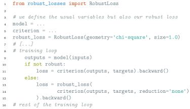
Figure 2: An example training loop in PyTorch where one can decide to use the robust training objective at the cost of three extra lines of code (lines 1, 6 and 13).

F.4 Experiment results

We complement the training curves in Figure 1 with comparisons of robust generalization metrics and training efficiency. In Figures 3 and 4 we show the training curves of Figure 1 along with two “robust” generalization metrics and two “average” performance metrics. For Digits, we consider the loss and accuracy on the worst sub-group—typically the typed digit 9—as the robust generalization metrics. For ImageNet, we look at the average loss (resp. accuracy) on the 10 labels with highest loss (resp. lowest accuracy). In each figure we also show the values achieved by ERM with two different regularization strengths chosen to optimize either loss or accuracy on the worst-subgroup. In Tables 5 and 6 we compare the number of epochs the various algorithms require to reach a training loss within 2% of the minimal value found across all runs. To achieve such convergence with the full batch method we run it for much longer: 30K epochs for Digits and 1K epochs for ImageNet.

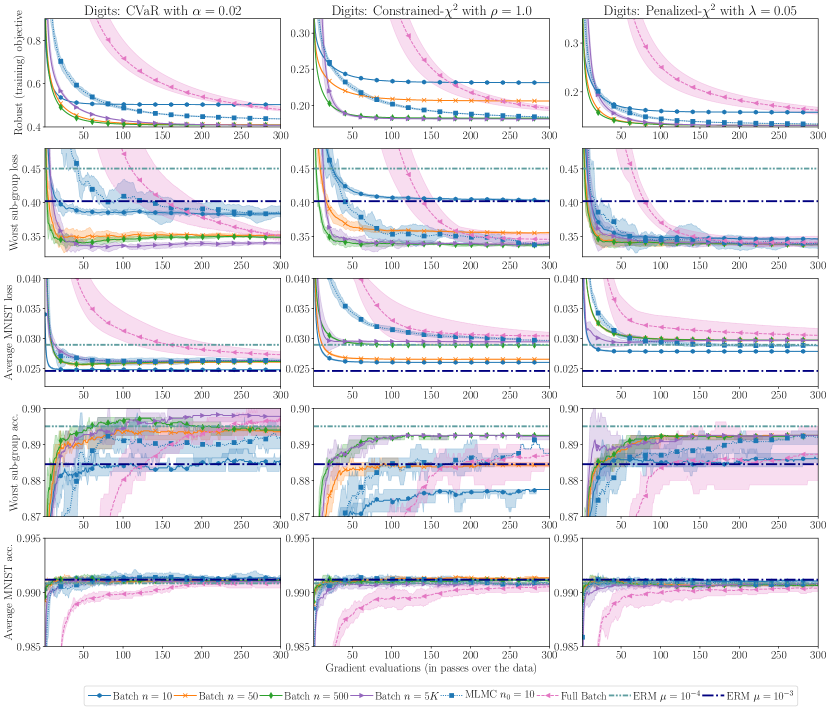
Figure 3: Detailed results from our digit recognition experiment. Shaded areas indicate range of variability across 5 repetitions (minimum to maximum), and the zoomed-in regions highlight the (often very small) “bias floor” of small batch sizes.

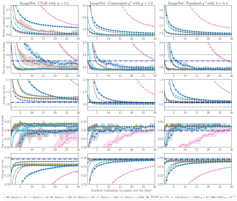
Figure 4: Detailed results from our ImageNet classification experiment. Shaded areas indicate range of variability across 5 repetitions (minimum to maximum), and the zoomed-in regions highlight the (often very small) “bias floor” of small batch sizes.

F.5 Discussion

F.5.1 Generalization performance

We now take a closer look at the curves presented in Figures 3 and 4. We first note that, in the context of machine learning, one does not wish to reach the minimum of the training objective but rather find a model that achieves good generalization performance. From that perspective, we observe that mini-batch methods achieve their best generalization performance in a shorter time than necessary to converge on the training objective, e.g., less than 50 epochs for CVaR on Digits when the training objective always requires more than 115 epochs.

In the case of Digits, we observe that DRO achieves a better trade-off than ERM in all settings. More precisely, DRO achieves better worst sub-group loss and accuracy than either of the ERM runs with no visible degradation in average accuracy and slightly worse average loss. We observe a similar trend in the case of ImageNet, albeit with a more visible degradation in average loss and accuracy.

We note that in the Digits experiment batch size $n=10$ has generalization performance more similar to ERM. This is an expected by-product of the bias inherent in small batch size, as in the edge case $n=1$, the mini-batch method degenerates to ERM.

Hu et al. [34] observe that applying DRO objectives of the form (18) directly on the 0-1 loss amounts to a simple monotonic transformation of the average accuracy, and is therefore equivalent to minimizing average accuracy. Thus, in as far as the logarithmic loss is a surrogate to the 0-1 loss (which is arguably the case in near realizable-settings), DRO might not provide improvements in robust accuracy. This is consistent with the observations in our experiments, where we see only small effects on the accuracy in the Digits experiments (which is close to realizable), and a somewhat more pronounced but still modest effect on ImageNet (which is not quite realizable, as the training accuracy is below 90%). Nevertheless, these observation do not preclude DRO from improvement the subpopulation test loss itself, as we see in our experiments: for Digits DRO provides between between 17.5% and 27% reduction in worst subgroup loss compared to ERM, and for ImageNet the reduction is a more modest 5.6% and 9%. While the common practice in machine learning is to view accuracy as the more important performance metric, logarithmic loss is also operationally meaningful, as it measures the calibration of the model predictions. Thus, DRO is potentially helpful in situations where robust precise uncertainty estimates are important.

We remark that approaches that explicitly target the subgroups on which we measure the generalization [e.g., 54] will likely perform better than DRO. However, in contrast to these methods DRO is agnostic to the subgroup definition—except that we use a subgroup validation set in order to tune its uncertainty set size—and therefore requires less data annotation.

F.5.2 Optimization performance

	Number of epochs to 2% of opt				Speed-up
	$n=50$	$n=500$	$n=5K$	Full-batch	vs. full-batch
$\mathcal{L}_{\textup{CVaR}},\alpha=0.02$	$189\pm 3$	$\boldsymbol{115}\pm 1$	$193\pm 4$	$1035$	$9.0\times$
$\mathcal{L}_{\chi^{2}},\rho=1$	$\infty$	$74\pm 1$	$\boldsymbol{60}\pm 3$	$570$	$9.5\times$
$\mathcal{L}_{\chi^{2}\textup{-pen}},\lambda=0.05$	$107\pm 1$	$\boldsymbol{104}\pm 1$	$131\pm 5$	$1680$	$16.2\times$

Table 5: Empirical complexity for the Digits experiment in terms of number of epochs required to reach within 2% of the optimal training objective value, averaged across 5 seeds $\pm$ one standard deviation. (For the full-batch experiments we only ran one seed). The “speed-up” column gives the ratio between the full batch complexity and the best mini-batch complexity.

	Number of epochs to 2% of opt							Speed-up
$n=$	$10$	$50$	$500$	$5K$	$50K$	$150K$	Full-batch	vs. full-batch
$\mathcal{L}_{\textup{CVaR}},\alpha=0.1$	$20$	$10$	$\boldsymbol{9}$	$\boldsymbol{9}$	$19$	-	$245$	$27\times$
$\mathcal{L}_{\chi^{2}},\rho=1$	$6$	$\boldsymbol{5}$	$\boldsymbol{5}$	$\boldsymbol{5}$	$8\pm 1$	$23$	$160$	$32\times$
$\mathcal{L}_{\chi^{2}\textup{-pen}},\lambda=0.4$	$7$	$\boldsymbol{5}$	$\boldsymbol{5}$	$\boldsymbol{5}$	$22$	$26$	$180$	$36\times$

Table 6: Empirical complexity for the ImageNet experiment in terms of number of epochs required to reach within 2% of the optimal training objective value, averaged across 5 seeds $\pm$ one standard deviation, whenever it is not zero. (For the full-batch experiments we only ran one seed). The “speed-up” column gives the ratio between the full batch complexity and the best mini-batch complexity.

As Figure 1 and Tables 5 and 6 indicate, mini-batch methods converge significantly faster than full-batch. We also see that, while theoretically optimal, MLMC methods are slower to converge. Furthermore, the bias is empirically much smaller than what the theory predicts and setting the batch size as small as 50 guarantees negligible bias; we investigate this further below. As the theory predicts, the MLMC method (for corresponding values of $n_{0}$) effectively counteracts this bias, and is able to converge to the optimal value even when $n_{0}$ is 10.

We also note that the effect of batch size on the depth of the algorithm (number of iterations) is remarkably consistent with the theoretical prediction of the variance-based analysis in Section 3: for smaller batch sizes the number of steps is roughly inversely proportional to the batch size, and the total amount of work is constant. The best stepsize also grows linearly with the batch size (see Table 4). As batch sizes grow, the best stepsize plateaus and the number of steps required for convergence also stops decreasing with the batch size, making the total work become larger.

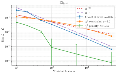
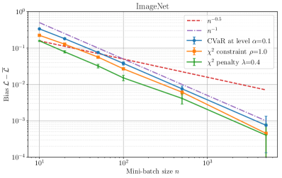
Figure 5: Evaluation of the bias $\mathcal{L}(\bar{x}_{T};P_{0})-\overline{\mathcal{L}}(\bar{x}_{T};n)$ at the last iterate $\bar{x}_{T}$ of the experiments in Figure 1, for different batch sizes $n$. (These batch sizes $n$ are not the same as the mini-batch size used to compute $\bar{x}_{T}$; we take the latter to be 10). Error bars indicate a 95% confidence interval computed using the bootstrap.

Bias analysis.

Figure 1 shows that even for small batch sizes—where the guarantees of Proposition 1 are essentially vacuous—stochastic gradient steps with the mini-batch gradient estimator find solutions very close to optimal. There could be two explanations for this finding: (a) $\mathcal{L}$ and $\overline{\mathcal{L}}$ are actually much closer to each other than the theory predicts, or (b) $\mathcal{L}$ and $\overline{\mathcal{L}}$ are far apart as expected, but still their minimizers are close.

To test hypothesis (a), we examine the loss values at the last iterate $\bar{x}_{T}$ of our Digits and ImageNet experiments with mini-batch size 10. For each objective, we estimate $\overline{\mathcal{L}}(\bar{x}_{T};n)$ for various values of $n$ by averaging 50K evaluations of $\mathcal{L}(\bar{x}_{T};S_{1}^{n})$, and use it to compute an estimate of the bias $\mathcal{L}(\bar{x}_{T};P_{0})-\overline{\mathcal{L}}(\bar{x}_{T};n)$. In Figure 5 we plot the bias estimate against the mini-batch size $n$. We see that hypothesis (a) is false: for both ImageNet and Digits, the difference $\mathcal{L}(\bar{x}_{T};P_{0})-\overline{\mathcal{L}}(\bar{x}_{T};n)$ is quite large at small $n$, as our upper bounds and matching lower bounds in the Bernoulli case would suggest. We also see that the bias decays as $1/n$ in all cases except for $\chi^{2}$ constraint in Digits; this is again consistent with our theory as we expect the inverse-cdf assumption to be relevant in practice and particularly for CVaR where it only needs to hold around the $1-\alpha$ quantile. We conclude that despite the significant bias at small batch size $n$, approximate minimizers of $\overline{\mathcal{L}}(x;n)$ are also approximate minimizers of $\mathcal{L}(x;P_{0})$. This is possibly due to the fact that the bias $\mathcal{L}(x;P_{0})-\overline{\mathcal{L}}(x;n)$ is nearly constant as a function of $x$. We leave further study of this hypothesis to future work.

F.6 Comparison with alternative optimization methods

We complement the worst-case complexity comparison in Table 1 by repeating our experiments with two alternative optimization methods: dual SGM and primal-dual methods.

F.6.1 Comparison with dual SGM

Experiment description.

Recall the dual SGM method we describe and analyze in Section A.3. The complexity guarantees of dual SGM depend quadratically on the size of the uncertainty set—scaling with $\alpha^{-2}$ for CVaR and with $\lambda^{-2}$ for the penalized version of the $\chi^{2}$ objective. In contrast, our theory predicts that the method we propose have an optimal linear dependence on the size of the uncertainty set. Here we empirically test this prediction on the Digits experiment. To do so, we compare the performance of our proposed mini-batch method with dual SGM for uncertainty sets of increasing size. For CVaR we consider

$$\alpha\in\{0.02,0.006,0.002,0.0006,0.0002\},$$

and for penalized $\chi^{2}$ we consider

$$\lambda\in\{0.05,0.015,0.005,0.0015,0.0005\}.$$

Parameter tuning.

For each uncertainty set size, we jointly tune the stepsizes $\gamma_{x}$ and $\gamma_{\eta}$ over the following grids

$$\gamma_{x}\in\{1\cdot 10^{-i},3\cdot 10^{-i}\}_{3\leq i\leq 6},\,\gamma_{\eta}\in\{1\cdot 10^{-i}\}_{2\leq i\leq 5}.$$

We choose a coarser grid for $\gamma_{\eta}$ as we noticed that the value of $\gamma_{\eta}$ had a marginal influence on the final performance. For both the mini-batch algorithm and dual SGM, we pick the batch size $n=500$ We follow the same averaging scheme and momentum as in our previous experiments.

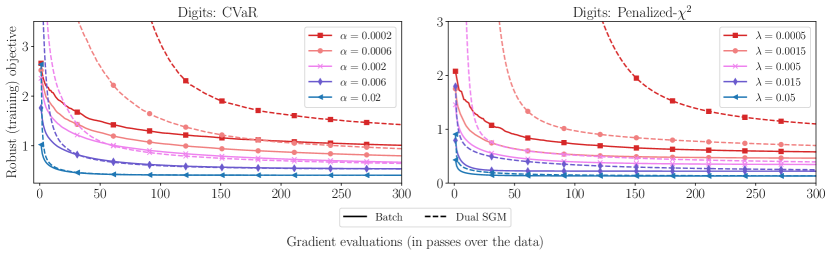
Figure 6: Comparison of batch methods to dual SGM on the digits experiments for increasing sizes of uncertainty set sizes or regularization. We observe that as the size grows, dual SGM performs increasingly worse.

Discussion of results.

We plot the results of the experiment in Figure 6. As the theory predicts, when the size of the uncertainty set grows, dual SGM performs significantly worse than batch methods. Conversely, as expected, for small uncertainty sets dual SGM performs on par with the mini-batch method. We empirically observe that the performance of dual SGM depends only weakly on the choice of $\gamma_{\eta}$. As a result, dual SGM is not much more difficult to tune than the mini-batch method.

F.6.2 Comparison with primal-dual methods

Experiment description.

We now turn to primal-dual methods, whose complexity guarantees scale as $\epsilon^{-2}$ but are linear in $N$, and are therefore expected to become less efficient as the size of the training set grows. To test this prediction, we repeat our Digits and ImageNet experiments (with $N=60.6$K and $N=1.2$M, respectively) using these alternative methods for the contrained-$\chi^{2}$ and CVaR objectives. We then compare their performance to that of gradient methods with our mini-batch estimator.

Method description.

Primal-dual methods maintain an iterate sequence $\{x_{t},q_{t}\}_{t\in\mathbb{N}}$, where $q_{t}\in\mathcal{U}(P_{0})\subset\Delta^{N}$ represent an online estimate of the distribution $q$ attaining the maximum in (6) at $x_{1},\ldots,x_{t}$. To compute $x_{t+1},q_{t+1}$, we sample a batch of $n$ indices $J_{1}^{n}$ drawn independently from $q_{t}$, and (denoting $S_{i}=s_{J_{i}}$) estimate the gradient of $\sum_{i=1}^{N}q_{i}\ell(x;s_{i})$ with respect to $x$ and $q$ as follows:

$$\tilde{g}^{x}_{t}=\frac{1}{n}\sum_{i=1}^{n}\nabla\ell(x_{t};S_{i})~{}~{}\mbox{and}~{}~{}[\tilde{g}^{q}_{t}]_{j}=\frac{1}{n}\sum_{i=1}^{n}\frac{1}{q_{J_{i}}}\ell(x_{t};S_{i})1_{\{J_{i}=j\}}.$$

To compute $x_{t+1}$ from $x_{t}$ and $\tilde{g}^{x}_{t}$ we apply the same stochastic gradient scheme we use in our previous experiments (Nesterov momentum 0.9). We also use the averaging scheme in [58] with parameter 3 as before. To compute $q_{t+1}$ from $q_{t}$ and $\tilde{g}^{q}_{t}$ we apply a mirror descent step. For the constrained $\chi^{2}$ problem the step is of the form

$$q_{t+1}=\operatorname*{arg\,max}_{q:\mathrm{D}_{\chi^{2}}(q,\frac{1}{N}\boldsymbol{1})\leq\rho}\left\{\left<q,\gamma_{q}\tilde{g}^{q}_{t}\right>+\frac{1}{2}\|q-q_{t}\|^{2}\right\}=\operatorname*{arg\,min}_{q\in\Delta^{N}:\|q-\frac{1}{N}\boldsymbol{1}\|^{2}\leq 2\rho/n}\|q-(q_{t}+\gamma_{q}\tilde{g}^{q}_{t})\|^{2},$$ (61)

i.e., a Euclidean projection of the unconstrained gradient step on $q_{t}$ to the uncertainty set. For the CVaR problem, the step is of the form

$$q_{t+1}=\operatorname*{arg\,max}_{q\in\Delta^{N}:\|q\|_{\infty}\leq\frac{1}{\alpha N}}\left\{\left<q,\mathrm{clip}(\gamma_{q}\tilde{g}^{q}_{t})\right>+\mathrm{D}_{\mathrm{kl}}(q,q_{t})\right\},$$ (62)

where $\mathrm{clip}(x)$ is the Euclidean projection of $x$ to $[-1,1]^{N}$.

The $\chi^{2}$ step is essentially the same as in [41], while the CvaR step is different from the proposal by Curi et al. [14]. Nevertheless, local norms regret analysis [11, 55] readily shows that with appropriate $\gamma_{x}$ and $\gamma_{q}$ the step (62) allows us to find $\epsilon$-optimal solutions within $\lesssim\frac{N\log\frac{1}{\alpha}B^{2}+G^{2}R^{2}}{\epsilon^{2}}$ iterations, similarly to the guarantee that Curi et al. [14] show for a computationally intractable determinantal point process scheme. They also propose a tractable approximation for this scheme, but do not prove that it converges to the solution of the CVaR problem.

Parameter tuning.

For every training task we jointly tune the parameters $\gamma_{x}$ and $\gamma_{q}$. We tune $\gamma_{x}$ over the values $10^{-i}$, $2\cdot 10^{-i}$ and $5\cdot 10^{-i}$ for $i\geq 1$ (similarly to our previous experiments) and we tune $\gamma_{q}$ over the values $10^{-i}$ and $3\cdot 10^{-i}$ for $i\geq 1$. The best-performing values of $(\gamma_{x},\gamma_{q})$ are $(0.02,0.003)$ for Digits/CVaR; $(0.02,3\cdot 10^{-7})$ for Digits/$\chi^{2}$; $(0.05,3\cdot 10^{-5})$ for ImageNet/CVaR; and $(0.02,3\cdot 10^{-11})$ for ImageNet/$\chi^{2}$. We use batch size $n=500$ throughout.

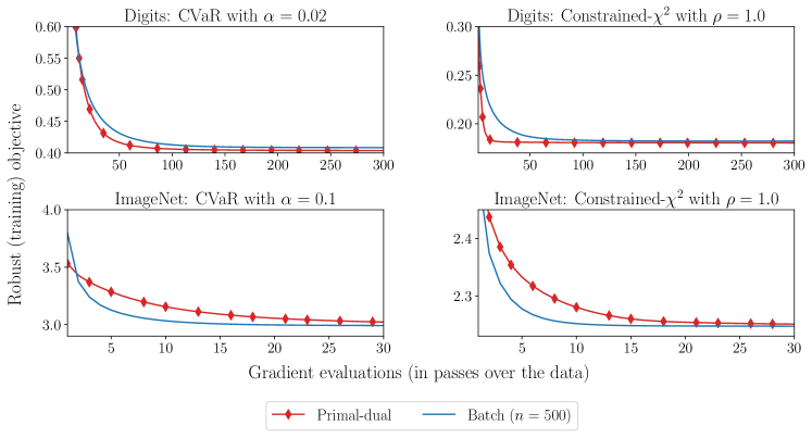
Figure 7: Comparison of batch methods to primal-dual methods. We observe that the primal-dual methods are more efficient on the Digits experiment, but the trend reverses on the large-scale ImageNet experiment.

Discussion of results.

Figure 7 compares primal-dual and mini-batch primal methods with the best-performing hyperparameters, for two datasets and two objectives. For the Digits experiment, the primal-dual method perform better that the primal-only method (for $\chi^{2}$ significantly so). This may appear surprising, since the primal-dual complexity guarantees are larger by an additional factor of $N=60.6$K for this dataset. However, a closer look at the analysis of primal-dual methods shows that the term $NB^{2}$ is actually an upper bound on $\sum_{i=1}^{N}[\ell(x;s_{i})]^{2}$ at $x=x_{1},x_{2},\ldots$. As the method converges, many data points are correctly classified with high confidence and therefore have very low value of $[\ell(x;s_{i})]^{2}$. Hence, a more realistic complexity estimate would replace $N$ by the number of incorrectly classified training points, which for Digits is quite small (less than 100). Moreover, we observe that the optimal value of $\gamma_{x}$ for primal-dual methods is significantly larger than the corresponding step size for the primal-only method, likely because $\tilde{g}^{x}$ gives uniform weights to each $s_{i}$ as opposed to the adversarial weight of the primal-only method. The larger step sizes enable more rapid optimization over $x$.

For the larger-scale ImageNet experiment, the primal-only method significantly outperforms the primal-dual method. This is consistent with the above discussion, since here the number of misclassified training examples is large (more than 100K).

As an additional illustration of the superior scalability of primal-only method, consider a thought experiment where we replicate each element in our dataset $m$ times to form a new dataset of size $mN$. Clearly, this will have no impact on the primal-only method. In contrast, the norm of $\tilde{g}^{q}$ will grow by a factor of $m$, and we may expect the complexity of the method to increase by that factor as well.

Finally, we remark that tuning the primal-dual method is considerably more difficult than tuning the primal-only method. In addition to having two learning rates to search over, using an overly large value for $\gamma_{q}$ typically causes the algorithm to converge to a suboptimal point rather than diverge. Therefore, the common procedure of decreasing the learning rate until divergence no longer occurs will fail for the primal-dual method.

References

- Ben-Tal et al. [2009] A. Ben-Tal, L. E. Ghaoui, and A. Nemirovski. Robust Optimization. Princeton University Press, 2009.
- Ben-Tal et al. [2013] A. Ben-Tal, D. den Hertog, A. D. Waegenaere, B. Melenberg, and G. Rennen. Robust solutions of optimization problems affected by uncertain probabilities. Management Science, 59(2):341–357, 2013.
- Bertsimas et al. [2011] D. Bertsimas, D. Brown, and C. Caramanis. Theory and applications of robust optimization. SIAM Review, 53(3):464–501, 2011.
- Bertsimas et al. [2018] D. Bertsimas, V. Gupta, and N. Kallus. Data-driven robust optimization. Mathematical Programming, Series A, 167(2):235–292, 2018.
- Blanchet and Kang [2020] J. Blanchet and Y. Kang. Semi-supervised Learning Based on Distributionally Robust Optimization, chapter 1, pages 1–33. John Wiley & Sons, Ltd, 2020. ISBN 9781119721871.
- Blanchet et al. [2019] J. Blanchet, Y. Kang, and K. Murthy. Robust Wasserstein profile inference and applications to machine learning. Journal of Applied Probability, 56(3):830–857, 2019.
- Blanchet and Glynn [2015] J. H. Blanchet and P. W. Glynn. Unbiased Monte Carlo for optimization and functions of expectations via multi-level randomization. In 2015 Winter Simulation Conference (WSC), pages 3656–3667. IEEE, 2015.
- Boucheron et al. [2013] S. Boucheron, G. Lugosi, and P. Massart. Concentration Inequalities: a Nonasymptotic Theory of Independence. Oxford University Press, 2013.
- Braun et al. [2017] G. Braun, C. Guzmán, and S. Pokutta. Lower bounds on the oracle complexity of nonsmooth convex optimization via information theory. IEEE Transactions on Information Theory, 63(7), 2017.
- Buolamwini and Gebru [2018] J. Buolamwini and T. Gebru. Gender shades: Intersectional accuracy disparities in commercial gender classification. In Conference on Fairness, Accountability and Transparency, pages 77–91, 2018.
- Clarkson et al. [2012] K. Clarkson, E. Hazan, and D. Woodruff. Sublinear optimization for machine learning. Journal of the Association for Computing Machinery, 59(5), 2012.
- Cressie and Read [1984] N. Cressie and T. R. Read. Multinomial goodness-of-fit tests. Journal of the Royal Statistical Society, Series B, pages 440–464, 1984.
- Csiszár [1967] I. Csiszár. Information-type measures of difference of probability distributions and indirect observation. Studia Scientifica Mathematica Hungary, 2:299–318, 1967.
- Curi et al. [2019] S. Curi, K. Levy, S. Jegelka, A. Krause, et al. Adaptive sampling for stochastic risk-averse learning. arXiv:1910.12511 [cs.LG], 2019.
- de Campos et al. [2009] T. E. de Campos, B. R. Babu, and M. Varma. Character recognition in natural images. In Proceedings of the Fourth International Conference on Computer Vision Theory and Applications, February 2009.
- Delage and Ye [2010] E. Delage and Y. Ye. Distributionally robust optimization under moment uncertainty with application to data-driven problems. Operations Research, 58(3):595–612, 2010.
- Duchi [2018] J. C. Duchi. Introductory lectures on stochastic convex optimization. In The Mathematics of Data, IAS/Park City Mathematics Series. American Mathematical Society, 2018.
- Duchi and Namkoong [2020] J. C. Duchi and H. Namkoong. Learning models with uniform performance via distributionally robust optimization. Annals of Statistics, to appear, 2020.
- Duchi et al. [2012] J. C. Duchi, P. L. Bartlett, and M. J. Wainwright. Randomized smoothing for stochastic optimization. SIAM Journal on Optimization, 22(2):674–701, 2012.
- Duchi et al. [2020] J. C. Duchi, T. Hashimoto, and H. Namkoong. Distributionally robust losses against mixture covariate shifts. arXiv:2007.13982 [cs.LG], 2020.
- Durrett [2019] R. Durrett. Probability: Theory and Examples, volume 49. Cambridge University Press, 2019.
- Efron and Stein [1981] B. Efron and C. Stein. The jackknife estimate of variance. The Annals of Statistics, 9(3):586–596, 1981.
- Esfahani and Kuhn [2018] P. M. Esfahani and D. Kuhn. Data-driven distributionally robust optimization using the Wasserstein metric: Performance guarantees and tractable reformulations. Mathematical Programming, Series A, 171(1–2):115–166, 2018.
- Fan et al. [2017] Y. Fan, S. Lyu, Y. Ying, and B. Hu. Learning with average top-k loss. In Advances in Neural Information Processing Systems 30, pages 497–505, 2017.
- Fuster et al. [2018] A. Fuster, P. Goldsmith-Pinkham, T. Ramadorai, and A. Walther. Predictably unequal? the effects of machine learning on credit markets. Social Science Research Network: 3072038, 2018.
- Ghosh et al. [2018] S. Ghosh, M. Squillante, and E. Wollega. Efficient stochastic gradient descent for distributionally robust learning. arXiv:1805.08728 [stats.ML], 2018.
- Giles [2008] M. B. Giles. Multilevel Monte Carlo path simulation. Operations research, 56(3):607–617, 2008.
- Giles [2015] M. B. Giles. Multilevel Monte Carlo methods. Acta Numerica, 24:259–328, 2015.
- Guzmán and Nemirovski [2015] C. Guzmán and A. Nemirovski. On lower complexity bounds for large-scale smooth convex optimization. Journal of Complexity, 31(1):1–14, 2015.
- Hashimoto et al. [2018] T. Hashimoto, M. Srivastava, H. Namkoong, and P. Liang. Fairness without demographics in repeated loss minimization. In Proceedings of the 35th International Conference on Machine Learning, 2018.
- He et al. [2016] K. He, X. Zhang, S. Ren, and J. Sun. Deep residual learning for image recognition. In Proceedings of the IEEE Conference on Computer Vision and Pattern Recognition, pages 770–778, 2016.
- Hendrycks and Dietterich [2019] D. Hendrycks and T. Dietterich. Benchmarking neural network robustness to common corruptions and perturbations. In Proceedings of the Seventh International Conference on Learning Representations, 2019.
- Hiriart-Urruty and Lemaréchal [1993] J. Hiriart-Urruty and C. Lemaréchal. Convex Analysis and Minimization Algorithms I. Springer, New York, 1993.
- Hu et al. [2018] W. Hu, G. Niu, I. Sato, and M. Sugiayma. Does distributionally robust supervised learning give robust classifiers? In Proceedings of the 35th International Conference on Machine Learning, 2018.
- Kalra and Paddock [2016] N. Kalra and S. M. Paddock. Driving to safety: How many miles of driving would it take to demonstrate autonomous vehicle reliability? Transportation Research Part A: Policy and Practice, 94:182–193, 2016.
- Kawaguchi and Lu [2020] K. Kawaguchi and H. Lu. Ordered SGD: A new stochastic optimization framework for empirical risk minimization. In Proceedings of the 23nd International Conference on Artificial Intelligence and Statistics, 2020.
- Kusuoka [2001] S. Kusuoka. On law invariant coherent risk measures. In Advances in Mathematical Economics, pages 83–95. Springer, 2001.
- Lan [2012] G. Lan. An optimal method for stochastic composite optimization. Mathematical Programming, Series A, 133(1–2):365–397, 2012.
- LeCun et al. [1995] Y. LeCun, L. D. Jackel, L. Bottou, A. Brunot, C. Cortes, J. S. Denker, H. Drucker, I. Guyon, U. A. Muller, E. Sackinger, P. Simard, and V. Vapnik. Comparison of learning algorithms for handwritten digit recognition. In International Conference on Artificial Neural Networks, pages 53–60, 1995.
- Motwani and Raghavan [1995] R. Motwani and P. Raghavan. Randomized Algorithms. Cambridge University Press, 1995.
- Namkoong and Duchi [2016] H. Namkoong and J. C. Duchi. Stochastic gradient methods for distributionally robust optimization with -divergences. In Advances in Neural Information Processing Systems 29, 2016.
- Nemirovski and Yudin [1983] A. Nemirovski and D. Yudin. Problem Complexity and Method Efficiency in Optimization. Wiley, 1983.
- Nemirovski et al. [2009] A. Nemirovski, A. Juditsky, G. Lan, and A. Shapiro. Robust stochastic approximation approach to stochastic programming. SIAM Journal on Optimization, 19(4):1574–1609, 2009.
- Nesterov [1983] Y. Nesterov. A method of solving a convex programming problem with convergence rate . Soviet Mathematics Doklady, 27(2):372–376, 1983.
- Nesterov [2004] Y. Nesterov. Introductory Lectures on Convex Optimization. Kluwer Academic Publishers, 2004.
- Nesterov [2005] Y. Nesterov. Smooth minimization of nonsmooth functions. Mathematical Programming, Series A, 103:127–152, 2005.
- Oakden-Rayner et al. [2020] L. Oakden-Rayner, J. Dunnmon, G. Carneiro, and C. Ré. Hidden stratification causes clinically meaningful failures in machine learning for medical imaging. In Proceedings of the ACM Conference on Health, Inference, and Learning, pages 151–159, 2020.
- Oren et al. [2019] Y. Oren, S. Sagawa, T. Hashimoto, and P. Liang. Distributionally robust language modeling. In Empirical Methods in Natural Language Processing (EMNLP), 2019.
- Paszke et al. [2017] A. Paszke, S. Gross, S. Chintala, G. Chanan, E. Yang, Z. DeVito, Z. Lin, A. Desmaison, L. Antiga, and A. Lerer. Automatic differentiation in pytorch. In Neural Information Processing Systems (NIPS) Workshop on Automatic Differentiation, 2017.
- Pitman [1993] J. Pitman. Probability. Springer-Verlag, 1993.
- Recht et al. [2019] B. Recht, R. Roelofs, L. Schmidt, and V. Shankar. Do ImageNet classifiers generalize to ImageNet? In Proceedings of the 36th International Conference on Machine Learning, 2019.
- Rockafellar and Uryasev [2000] R. T. Rockafellar and S. Uryasev. Optimization of conditional value-at-risk. Journal of Risk, 2:21–42, 2000.
- Russakovsky et al. [2015] O. Russakovsky, J. Deng, H. Su, J. Krause, S. Satheesh, S. Ma, Z. Huang, A. Karpathy, A. Khosla, M. Bernstein, A. C. Berg, and L. Fei-Fei. ImageNet large scale visual recognition challenge. International Journal of Computer Vision, 115(3):211–252, 2015.
- Sagawa et al. [2020] S. Sagawa, P. W. Koh, T. B. Hashimoto, and P. Liang. Distributionally robust neural networks for group shifts: On the importance of regularization for worst-case generalization. In Proceedings of the Eighth International Conference on Learning Representations, 2020.
- Shalev-Shwartz [2012] S. Shalev-Shwartz. Online learning and online convex optimization. Foundations and Trends in Machine Learning, 4(2):107–194, 2012.
- Shalev-Shwartz and Singer [2006] S. Shalev-Shwartz and Y. Singer. Convex repeated games and fenchel duality. In Advances in Neural Information Processing Systems 19, 2006.
- Shalev-Shwartz and Wexler [2016] S. Shalev-Shwartz and Y. Wexler. Minimizing the maximal loss: How and why? In Proceedings of the 33rd International Conference on Machine Learning, 2016.
- Shamir and Zhang [2013] O. Shamir and T. Zhang. Stochastic gradient descent for non-smooth optimization: Convergence results and optimal averaging schemes. In Proceedings of the 30th International Conference on Machine Learning, pages 71–79, 2013.
- Shapiro [2017] A. Shapiro. Distributionally robust stochastic programming. SIAM Journal on Optimization, 27(4):2258–2275, 2017.
- Shapiro et al. [2009] A. Shapiro, D. Dentcheva, and A. Ruszczyński. Lectures on Stochastic Programming: Modeling and Theory. SIAM and Mathematical Programming Society, 2009.
- Sinha et al. [2018] A. Sinha, H. Namkoong, and J. Duchi. Certifying some distributional robustness with principled adversarial training. In Proceedings of the Sixth International Conference on Learning Representations, 2018.
- Staib and Jegelka [2019] M. Staib and S. Jegelka. Distributionally robust optimization and generalization in kernel methods. In Advances in Neural Information Processing Systems 32, pages 9134–9144, 2019.
- Torralba and Efros [2011] A. Torralba and A. A. Efros. Unbiased look at dataset bias. In Proceedings of the IEEE Conference on Computer Vision and Pattern Recognition, pages 1521–1528. IEEE, 2011.
- Trindade et al. [2007] A. A. Trindade, S. Uryasev, A. Shapiro, and G. Zrazhevsky. Financial prediction with constrained tail risk. Journal of Banking & Finance, 31(11):3524–3538, 2007.
- van Erven and Harremoës [2014] T. van Erven and P. Harremoës. Rényi divergence and Kullback-Leibler divergence. IEEE Transactions on Information Theory, 60(7):3797–3820, 2014.
- Wainwright [2019] M. J. Wainwright. High-Dimensional Statistics: A Non-Asymptotic Viewpoint. Cambridge University Press, 2019.
- Wang et al. [2020] S. Wang, W. Guo, H. Narasimhan, A. Cotter, M. Gupta, and M. I. Jordan. Robust optimization for fairness with noisy protected groups. arXiv:2002.09343 [cs.LG], 2020.
- Yu [1997] B. Yu. Assouad, Fano, and Le Cam. In Festschrift for Lucien Le Cam, pages 423–435. Springer-Verlag, 1997.
- Zinkevich [2003] M. Zinkevich. Online convex programming and generalized infinitesimal gradient ascent. In Proceedings of the Twentieth International Conference on Machine Learning, 2003.