Entanglement generation in quantum thermal machines

Abstract

We show that in a linear quantum machine, a driven quantum system that evolves while coupled with thermal reservoirs, entanglement between the reservoir modes is unavoidably generated. This phenomenon, which occurs at sufficiently low temperatures and is at the heart of the third law of thermodynamics, is a consequence of a simple process: the transformation of the energy of the driving field into pairs of excitations in the reservoirs. For a driving with frequency $\omega_{d}$ we show entanglement exists between environmental modes whose frequencies satisfy the condition $\omega_{i}+\omega_{j}=\omega_{d}$. We show that this entanglement can persist for temperatures that can be significantly higher than the lowest achievable ones with sideband resolved cooling methods.

I Introduction

Quantum thermodynamics andersVinjanampathy ; kosloff ; brandaoHorodeckiNg is an emerging field whose goal is to study the exchange of heat and work in the quantum domain. In recent years novel thermal machines operating at the atomic scale have been built using various technologies. These include, most notably, ion traps eschnerMorigiSchmidt ; abahRossnagelJacob ; maslennikovDingHablutzel and superconducting qubits karimiPekolaCampisi . Although a first principle description of such devices needs to be based on quantum laws, a study of their performance revealed that they satisfy the same constraints imposed by classical thermodynamics (for example, their efficiency is bounded by the Carnot limit) allahverdyanHovhannisyanJanzing ; levyAlickiKosloff ; wuSegalBrumer ; ticozziViola ; masanesOppenheim ; wilmingGallego ; skrzypczykBrunnerLinden . Although it is reassuring that classical results are reobtained from a quantum treatment, this naturally raises a troubling question: what is quantum in quantum thermodynamics? uzdinLevyKosloff . More precisely: are there thermodynamical tasks that are possible (or impossible) because of quantum effects? (or: are there quantum effects that are unavoidably associated with thermodynamical cycles?). Even though, in this context, the role of quantum coherences kammerlanderAnders , correlations sapienzaCerisolaRoncaglia , and entanglement brunnerHuberLinden ; bohrBraskHaackBrunner ; khandelwalPalazzoBrunner as thermodynamical resources have been recently studied, in our opinion, the answer to the above questions is still inconclusive. Here we show that quantum entanglement plays a central role in thermodynamics: we prove that when work is performed on a system $\mathcal{S}$, which is in contact with reservoirs $\mathcal{E}_{R}$ and $\mathcal{E}_{L}$, time-extensive entanglement between environmental degrees of freedom is unavoidable at sufficiently low temperatures.

Hints about the existence of this entanglement, induced by the driving, were found in pazFreitas17 ; pazFreitas18 while studying the nature of the heat flow between the environments. It was shown that in the stationary regime the energy stored in each environment varies due to two processes. First, the resonant absorption (or emission) from (or into) the driving field can transport an excitation in a mode with frequency $\omega_{i}$ to a mode with frequency $\omega_{i}+k\omega_{d}$, where $\omega_{d}$ is the driving frequency and $k$ is an integer number. Naturally, this process is not present at zero temperature, where there are no excitations to be transported around. Thus, at very low temperature, the environmental energy varies because of a different process: the energy of the driving is dumped into two modes whose frequencies satisfy the condition $\omega_{i}+\omega_{j}=k\omega_{d}$. In pazFreitas17 ; pazFreitas18 this was interpreted as the non-resonant creation of a pair of excitations, one in each mode, a process similar to the one underlying the dynamical Casimir effect dodonov ; wilsonJohanssonPourkabirian . However, the arguments in pazFreitas17 ; pazFreitas18 are a conjecture and not a proof of the existence of entangled pairs. Here we present a rigorous proof of this fact by showing that the environmental modes become entangled below a certain temperature. Moreover we show that entanglement can persist for temperatures which are higher than the lowest achievable ones by physically relevant cooling methods (analyzing both the resolved sideband and Doppler limits). Although our proof restricts to linear quantum open systems martinezPaz (see below), as the process responsible for the generation of entanglement is the same enforcing the validity of the third law of thermodynamics pazFreitas17 ; pazFreitas18 , it is natural to conjecture that our result is not a mere consequence of linearity but a general one.

The paper is organized as follows: In Section 2 we present our model, which is a generalization of the standard quantum Brownian motion (QBM) model including a time-dependant driving field, and present its formal solution. In Section 3 we show how to explicitly solve this model for the case of a periodic driving using Floquet theory. In Section 4 we use the previous results to compute correlation functions between different environmental modes and we discuss their properties in the long time regime. In Section 5 we study the entanglement between environmental modes at zero and non-zero environmental temperature. We provide a simple analitycal expression to compute an entanglement measure (the logarithmic negativity) that shows entanglement is created at a constant speed (time extensivity) in a physically relevant range of parameters. We also provide a simple formula to predict the temperature at which entanglement vanishes due to thermal excitations. We summarize our results in Section 6.

II The model

We consider the following generalization of the quantum Brownian motion model huPazZhang ; caldeiraLeggett : a system $\mathcal{S}$ (a parametric oscillator with coordinate $x$) is coupled with an environment $\mathcal{E}$ formed by independent oscillators (whose coordinates are denoted as $q_{i}$, with $i=1,\dots,N$). The environment is divided into two pieces $\mathcal{E}_{\alpha}$, where $\alpha=R,L$, each of which consists of the oscillators $q_{i}$ with $i\in\mathcal{E}_{\alpha}$. Each $\mathcal{E}_{\alpha}$ is initially prepared in a thermal state with temperature $T_{\alpha}$. This model represents the physical situation shown in Figure (1).

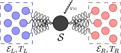
Figure 1: A parametric oscillator $\mathcal{S}$ driven by $V\left(t\right)$ is coupled with two environments $\mathcal{E}_{L}$ and $\mathcal{E}_{R}$ at temperatures $T_{L}$ and $T_{R}$, respectively.

Thus, our model describes the closed Universe formed by the system $\mathcal{S}$ and the environment $\mathcal{E}$, whose dynamics is governed by the total Hamiltonian $H_{T}=H_{\mathcal{S}}+H_{\mathcal{E}}+H_{\mathcal{S},\mathcal{E}}$. Here, the system’s Hamiltonian is $H_{\mathcal{S}}=p^{2}/2m+mV(t)x^{2}/2$ while the environmental and interaction terms are, respectively, $H_{\mathcal{E}}=\sum_{i}\left(p_{i}^{2}/2m_{i}+m_{i}\omega_{i}^{2}q_{i}^{2}/2\right)$ and $H_{\mathcal{S},\mathcal{E}}=x\sum_{i}\lambda_{i}q_{i}$. An important feature of the environment is its spectral density $I\left(\omega\right)=\sum_{i}\lambda_{i}^{2}\delta\left(\omega-\omega_{i}\right)/m_{i}\omega_{i}$ (the spectral density of each $\mathcal{E}_{\alpha}$ is denoted as $I_{\alpha}\left(\omega\right)$ and is defined in the same way, restricting the summation to $i\in\alpha$). As we are insterested in studying correlations between the environmental modes, we will solve this model in a way which is different from the one used in standard treatments of QBM huPazZhang . Thus, we solve the full Heisenberg equations of motion of the coupled system, which read

$$\begin{dcases}\ddot{q}_{i}+\omega_{i}^{2}\,q_{i}=-\lambda_{i}\,x/m_{i}&\quad i=1,\dots,N\\ \ddot{x}+V\left(t\right)x=-\textstyle{\sum_{i=1}^{N}}\lambda_{i}\,q_{i}/m&\end{dcases}$$ (1)

Interestingly the above equations can be formally solved and the solutions expressed in terms of two decoupled sets of operators. One of them, which we denote $q_{i}^{h}\left(t\right)$, acts on the environmental state space, and the other one, which we denote $x_{h}\left(t\right)$, acts on the system state space. The operators $q_{i}^{h}\left(t\right)$ are the free Heisenberg operators of the environmental modes

$$q_{i}^{h}(t)=q_{i,0}\cos\left(\omega_{i}t\right)+p_{i,0}\sin\left(\omega_{i}t\right)/m_{i}\omega_{i},$$ (2)

where $q_{i,0}$ and $p_{i,0}$ are Schröedinger operators. In turn, $x_{h}\left(t\right)$ is a dressed operator for $\mathcal{S}$ that satisfies the linear equation

$$\ddot{x}_{h}+V_{R}\left(t\right)x_{h}+\gamma\ast\dot{x}_{h}=0,$$ (3)

where the notation $F\ast f=\int_{0}^{t}dt^{\prime}F\left(t,t^{\prime}\right)f\left(t^{\prime}\right)$ is used. Above, $\gamma$ is the dissipation kernel defined as $\gamma\left(t,t^{\prime}\right)=\int d\omega\,I\left(\omega\right)\cos\left[\omega\left(t-t^{\prime}\right)\right]/m\omega$, and $V_{R}\left(t\right)=V\left(t\right)-\gamma\left(0\right)$ is the renormalized potential. The solution of the full Heisenberg equations (1) is

$$\begin{dcases}q_{i}&=q_{i}^{h}+K_{ij}^{\left(1\right)}\ast q_{j}^{h}+K^{\left(2\right)}_{i}\ast x_{h},\\ x&=x_{h}+K^{\left(3\right)}_{j}\ast q_{j}^{h},\end{dcases}$$ (4)

where a summation over repeated indices is implicit. The kernel $K^{\left(1\right)}$, which plays a central role in our calculations, is

$$K_{ij}^{\left(1\right)}\left(t,t^{\prime}\right)=\lambda_{i}\lambda_{j}\int_{t^{\prime}}^{t}d\tau\sin\left[\omega_{i}\left(t-\tau\right)\right]G\left(\tau,t^{\prime}\right)/mm_{i}\omega_{i},$$ (5)

where $G$ is the Green function of Eq. (3) above. The other two kernels are

$$\begin{dcases}K_{i}^{\left(2\right)}\left(t,t^{\prime}\right)&=-\lambda_{i}\,\text{sin}\left[\omega_{i}\left(t-t^{\prime}\right)\right]/m_{i}\,\omega_{i}\\ K_{j}^{\left(3\right)}\left(t,t^{\prime}\right)&=-\lambda_{j}\,G\left(t,t^{\prime}\right)/m.\end{dcases}$$ (6)

So far the expressions we obtained for $q(t)$ and $x(t)$ are exact. To compute them explicitly we need to solve the equation for $G$, a task that is feasible for certain spectral densities and for simple forms of $V(t)$ (In fact, once we do this we can express $x_{h}(t)$ as a linear combination of the Schrödinger operators $x_{0}$ and $p_{0}$). In the case of constant $V(t)$, the expressions presented in Eq. (4) can be used to obtain all the known results for the standard QBM model, and also to compute environmental correlations. Below we will discuss the solution for a time-periodic driving field.

III Solution for periodic driving using Floquet theory

In order to deal with the explicit time dependence induced by $V\left(t\right)$ we use Floquet theory. For a periodic driving with $V\left(t\right)=\sum_{k}V_{k}e^{ik\omega_{d}t}$, $G\left(t,t^{\prime}\right)$ can always be written as

$$G\left(t,t^{\prime}\right)=\textstyle{\sum_{k}}A_{k}\left(t-t^{\prime}\right)e^{ik\omega_{d}t},$$ (7)

where $A_{k}$ vanishes for negative arguments. For $G$ to be a Green fuction of Eq. (3), $A_{k}$ must satisfy a linear set of coupled differential equations. Instead of explicitly writing this system, we will simply present an equivalent one involving their Laplace transform $\tilde{A}_{k}(s)=\int_{0}^{\infty}dt\,A_{k}\left(t\right)\,e^{-st}$:

$$\tilde{g}^{-1}\left(s+ik\omega_{d}\right)\tilde{A}_{k}\left(s\right)+\textstyle{\sum_{n\neq 0}}V_{n}\,\tilde{A}_{k-n}\left(s\right)=\delta_{k0}.$$ (8)

Here, $\tilde{g}$ is the Laplace transform of the static Green function (obtained when $V\left(t\right)=V_{0}$), which is $\tilde{g}^{-1}\left(s\right)=s^{2}+\omega_{r}^{2}+s\,\tilde{\gamma}\left(s\right)$ (where $\omega_{r}^{2}=V_{0}-\gamma\left(0\right)$ is the renormalized frequency and $\tilde{\gamma}$ is the Laplace transform of $\gamma$). The above system of equations can be simply solved by using a perturbative series expansion which is valid when the Fourier coefficients of the potential $\lvert V_{k}\rvert$ are small. The validity of this approximation also requires the frequency of the driving $\omega_{d}$ to be detuned from the parametric resonance. Thus, the solution of (8) satisfies the following recurrence relation:

$$A_{k}^{\left(m\right)}\!\left(s\right)=\tilde{g}\left(s+ik\omega_{d}\right)[\delta_{k0}-\textstyle{\sum_{n\neq 0}}V_{n}\,\tilde{A}_{k-n}^{\left(m-1\right)}\left(s\right)],$$ (9)

for $m\geq 1$, with $A_{k}^{\left(0\right)}\left(s\right)=\tilde{g}\left(s+ik\omega_{d}\right)\,\delta_{k0}$. It is interesting to note that the coefficientes $\tilde{A}_{k}$ satisfy certain properties which can be interpreted as a generalization of the static fluctuation-dissipation relation to the driven case. After some algebraic manipulations one can show that

$$\text{Im}[\tilde{A}_{0}\left(i\omega\right)]=-\pi\textstyle{\sum_{k}}I\left(\omega-k\omega_{d}\right)\,\lvert\tilde{A}_{k}\left[i\left(\omega-k\omega_{d}\right)\right]\rvert^{2}/2m.$$ (10)

In the static case, when $V_{k}=0\quad\forall\lvert k\rvert\geq 1$ , it reduces to

$$\text{Im}[\tilde{g}\left(i\omega\right)]=-\pi I\left(\omega\right)\left\lvert\tilde{g}\left(i\omega\right)\right\rvert^{2}/2m,$$ (11)

which is the well known expression for the fluctuation-dissipation relation in the absence of a driving field huPazZhang . Bellow we will use the above equations to compute correlations between environmental modes. It is worth noticing that the generalized fluctuaton-dissipation relation considerably simplifies the expressions for the correlators and determines some of their most interesting properties.

IV Correlation functions between environmental bands

We use Eq. (4) to compute all correlation functions between two environmental bands: one of them consists of oscillators whose frequencies are distributed around $\omega_{i}$ (with a bandwidth $\Delta\omega$) and the other (disjoint) one is centered around $\omega_{j}$. Expressions below will depend on the product $I(\omega)\Delta\omega$ which, for sufficiently small values of $\Delta\omega$, plays the role of an effective coupling strength between the reservoir band and $\mathcal{S}$ (since $I(\omega)\Delta\omega\approx\lambda^{2}/m\omega$). We can show that the environmental correlators can be expressed as the sum of a term that depends on the initial state of $\mathcal{S}$ and another one that depends on the initial correlations within $\mathcal{E}$. In fact, when a stable stationary regime exists, the dependance on the initial conditions for $x$ becomes irrelevant and the dynamics is dominated by the term involving the initial correlations within $\mathcal{E}$. The existence of such regime requires the energy pumped into $\mathcal{S}$ to be dissipated by $\mathcal{E}$, which can be achieved for small driving amplitudes, provided that $\omega_{d}$ is detuned from the parametric resonance. In Appendix A we include the general form of the equal time correlators $\left\langle\left\{q_{i}\left(t\right),q_{j}\left(t\right)\right\}\right\rangle$, both at zero and non-zero environmental temperatures which, together with the expression for the momentum and the cross-correlators, will be used below to compute a measure of entanglement between environmental bands. Here, for the sake of simplicity, we show just an expression that enables us to discuss a feature that is common to all correlators which in a physically relevant regime become time-extensive. Thus, we compute the energy $E_{i}$ stored in the band $\omega_{i}$, with $i\in\alpha$, which is the sum of the two diagonal correlators. It has the following form in the long time limit:

$$E_{i}(t)\rightarrow\left[1/2+n_{\alpha}\left(\omega_{i}\right)\right]\omega_{i}+\dot{\mathcal{Q}}_{i}\times t,$$ (12)

with

$$\frac{\dot{\mathcal{Q}}_{i}}{\Delta\omega}=\textstyle{\sum_{k}}\textstyle{\sum_{\alpha^{\prime}}}\omega_{i}\left\{\Theta\left(\omega_{i,k}\right)p_{\alpha,\alpha^{\prime}}^{(k)}\left(\omega_{i}\right)\left[n_{\alpha^{\prime}}\left(\omega_{i,k}\right)-n_{\alpha}\left(\omega_{i}\right)\right]\right.$$ (13)

$$\left.+\Theta\left(-\omega_{i,k}\right)p_{\alpha,\alpha^{\prime}}^{(k)}\left(\omega_{i}\right)\left[n_{\alpha^{\prime}}\left(\left\lvert\omega_{i,k}\right\rvert\right)+n_{\alpha}\left(\omega_{i}\right)+1\right]\right\},$$

where $\omega_{i,k}=\omega_{i}-k\omega_{d}$, $\Theta$ is the step function, $n_{\alpha}\left(\omega\right)$ is the Planck distribution with temperature $T_{\alpha}$, and $p_{\alpha,\alpha^{\prime}}^{(k)}\left(\omega_{i}\right)=\pi\,I_{\alpha}\left(\omega_{i}\right)I_{\alpha^{\prime}}\left(\left\lvert\omega_{i,k}\right\rvert\right)\lvert\tilde{A}_{k}\left(i\omega_{i,k}\right)\rvert^{2}/2m^{2}$ is the probability that mode $\omega_{i}$ in $\mathcal{E}_{\alpha}$ interacts with mode $\omega_{i,k}$ in $\mathcal{E}_{\alpha^{\prime}}$ through $\mathcal{S}$. Remarkably, $E_{i}$ is a linear function of time, a feature that is common to all correlators. This is really a consequence of the continuum hypothesis for $\mathcal{E}$ since any discrete environment has recurrence times $t_{rec}\approx 1/\delta\omega$, where $\delta\omega$ is the smallest frequency splitting in $\mathcal{E}$. Therefore, although the above expression is valid for long times, it is not valid for arbitrarily long times (the continuum hypothesis for arbitrarily long times, which is equivalent to assuming an infinite heat capacity for each band, yields non-physical covariance matrices). Technically, time extensivity is obtained in two steps: (i) we write all second order correlators as frequency integrals (using Eq. (4) and transforming the summations over discrete modes into integrals over $\omega$, weighted by $I(\omega)$); (ii) we collapse the frequency integrals using the fact that terms involving the kernels $K_{ij}^{(1)}$ become highly peaked functions of $\omega$ in the long time limit (that can be treated as Dirac $\delta$-functions until the time for which the discreteness of the environmental spectrum becomes relevant).

In Eq. (13) we can see the hints pointing towards the existence of entanglement that motivated our current study. The first term in its r.h.s. involves the interaction of a mode $\omega_{i}$ and another one with frequency $\omega_{i}-k\omega_{d}$, and describes resonant transport (which can induce either heating or cooling of the modes, depending on the relation between their populations). To the contrary, the second term, which being positive is always associated with heating, involves the interaction between modes whose frequencies add up to a multiple of $\omega_{d}$. This spliting of the driving energy between two modes motivated us to ask if entanglement is generated between them. We will show below that this is indeed the case. Before that, let us mention that our exact formula (which takes into account the initial transient and does not involve any time averaging) can be used to obtain Fig. (2), where we show the behavior of $E_{i}(t)$ for an Ohmic spectral density $I(\omega)=2m\gamma_{0}\omega\Lambda^{2}/\pi(\omega^{2}+\Lambda^{2})$ and a harmonic driving $V_{R}(t)=\omega_{r}^{2}+V\cos(\omega_{d}t)$. The plot (that corresponds to the case where $T_{R}=T_{L}=0$) shows a linear behavior for long times, with a modulation with frequency $\omega_{d}$.

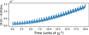
Figure 2: Energy of the mode $\omega_{i}$ as a function of time at zero temperature, for $\omega_{i}=\omega_{d}-\delta$. Here, $\omega_{d}=\omega_{r}-\delta$ with $\delta=10\gamma_{0}$, $\omega_{r}=800\gamma_{0}$, $V=\omega_{r}^{2}/32$, $m=10m_{i}$ $t=20\gamma_{0}$ and $\gamma_{0}=0.005$.

In the next section we will discuss entanglement between environmental modes focusing on the long (but not infinitly long) time limit, where time extensivity dominates.

V Entanglement between environmental bands

Here we will study entanglement between two environmental bands which are respectively centered around frequencies $\omega_{i}$ and $\omega_{j}$, with $i\in\mathcal{E}_{R}$ and $j\in\mathcal{E}_{L}$. For this we will compute a standard measure of entanglement, which is obtained from the reduced density matrix of the two modes $i$ and $j$. We will use the logaritmic negativity $E_{\mathcal{N}}\left(t\right)$ which is a good measure of entanglement since the two-mode state in the stationary regime is Gaussian adessoIlluminati . $E_{\mathcal{N}}\left(t\right)$ is obtained, as it is well known adessoIlluminati ; serafiniIlluminatiSiena , from the smallest symplectic eigenvalue of the covariance matrix corresponding to the partially transposed reduced density matrix of $i$ and $j$. We will obtain our results using two complementary methods. On the one hand, we will derive analytic expressions for $E_{\mathcal{N}}\left(t\right)$, which are valid in the limit of small driving and weak coupling. On the other hand, we will numerically evaluate our exact analytic expressions and compare them with the above aproximation. In the following subsections we will first discuss the case where the environmental temperatures vanish and show that entanglement exists only for modes satisfying the condition $\omega_{i}+\omega_{j}=\omega_{d}$. Then we will present the generalization of this result for the non-zero temperature case. In both cases we will analyze in detail the nature of the results for physically relevant ranges of parameters ($\omega_{d}$, $\omega_{r}$ and $\gamma_{0}$) describing the most interesting cases that correspond to the resolved sideband and Doppler limits (see below). In the last subsection we present a formula that allows us to compute the maximum temperature at which entanglement between the environmental bands is still present.

V.1 Entanglement at zero temperature

We compute the long time limit of the average value of $E_{\mathcal{N}}\left(t\right)$ between two bands whose frequencies add up to a multiple of the driving frequency $\omega_{d}$ (where the average is taken over a driving cycle). Using the above expressions we show that

$$E_{\mathcal{N}}\left(t\right)=\Gamma_{0}\times t,$$ (14)

where

$$\Gamma_{0}=\frac{1}{m}\Delta\omega\left\lvert V\right\rvert\sqrt{I_{R}(\omega_{i})I_{L}(\omega_{j})}\left\lvert\text{Re}\left[\tilde{g}_{i}\,\tilde{g}^{\ast}_{j}\right]\right\rvert,$$ (15)

with $\tilde{g}_{l}=\tilde{g}\left(i\omega_{l}\right)$. This formula, which is valid to leading order in $V$ in the weak damping regime, shows that the driving creates entanglement at a constant speed. This is one of the central results of this paper. Instead, if $\omega_{i}+\omega_{j}=\omega_{d}+\epsilon$ with $\epsilon\ll\omega_{d}$, we find that $E_{\mathcal{N}}\left(t\right)\propto\left\lvert\text{sinc}\left(\epsilon t\right)\right\rvert\,t$, which is a rapidly decaying function of $\epsilon$ whose amplitude does not grow with time. It is interesting to compare the time dependence of the entanglement with the one of the energy. Although they are both linear in time they display significant differences. Thus, in the same regime described above, Eq. (12) can be rewritten as $E_{i}\left(t\right)=\omega_{i}/2+\dot{\mathcal{Q}}_{i}\times t$ where $\dot{\mathcal{Q}}_{i}=\pi\omega_{i}\Delta\omega\left\lvert V\right\rvert^{2}I_{R}\left(\omega_{i}\right)I\left(\omega_{j}\right)\lvert\tilde{g}_{i}\,\tilde{g}^{\ast}_{j}\rvert^{2}/2m^{2}$. Notably, the speed with which the energy grows is of second order in $V$. Instead, as the entanglement grows when cross-correlations develop, $\Gamma_{0}$ turns out to be of first order in the driving amplitude. It is worth mentioning that $E_{\mathcal{N}}\left(t\right)$ is proportional to the environmental bandwith $\Delta\omega$. This is a natural result since entanglement is stablished between modes satisfying the matching condition $\omega_{i}+\omega_{j}=\omega_{d}$. Therefore, $E_{\mathcal{N}}\left(t\right)$ should be proportional to the number of entangled pairs which is linear in $\Delta\omega$.

The amount of entanglement produced at a certain time depends on the frequencies of both modes. By analyzing the dependence of the entanglement (as measured by the logarithmic negativity) as a function of ($\omega_{i},\omega_{j}$) we can understand the relevance of our result in the various regimes defined by the relation between $\omega_{d}$, $\omega_{r}$ and $\gamma_{0}$. For example, if $\omega_{d}=\omega_{r}-\delta$ with $\delta\gg\gamma_{0}$ a maximum of entanglement is expected for $\omega_{i}$ close to $\omega_{r}-\omega_{d}=\delta$. This is because oscillators in such band are in the “resolved sideband” limit as the decay rate is $\gamma_{0}\ll\omega_{i}$ ($\omega_{r}\gg\gamma_{0}$ is implicit). In this regime the dominant process is the creation of a pair of phonons, one in the mode $\omega_{i}$ and another one in the mode $\omega_{j}=\omega_{d}-\omega_{i}=\omega_{r}-2\delta$. This is the pair production mechanism that, as discussed in pazFreitas18 , sets the limit for the lowest achievable temperature in sideband resolved cooling methods. This intuitive picture is confirmed by an exact numerical evaluation of the entanglement, shown in Fig. 3 (a) where these spectral peaks can be clearly seen. Dimensional analysis of Eq. (15) provides us with a natural unit of entanglement $E_{0}=\gamma_{0}\Delta\omega V/\omega_{r}^{3}$, which we use to normalize our plots. The agreement between the exact numerical evaluation and the above analytic estimate is remarkable.

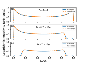
Figure 3: Dependence of the logarithmic negativity $E_{\mathcal{N}}/E_{0}$ on the frequency $\omega_{i}$ in the resolved side-band limit when $\omega_{i}+\omega_{j}=\omega_{d}$. (a): When both environments are at zero temperature two peaks and a broadband plateau are clearly visible. (b): When $T_{L}$ is raised to $T_{L}=10\gamma_{0}$ the peak at the right of the figure (that couples with low frequency oscillators in $\mathcal{E}_{L}$) dissappears. (c): When $T_{R}=T_{L}=10\gamma_{0}$ only the central plateau is left. In all cases the exact result -blue line- coincides with the analytical estimate given in (15) and (17). We used the parameters $\omega_{d}=\omega_{r}-\delta$ with $\delta=10\gamma_{0}$, $\omega_{r}=800\gamma_{0}$, $V=\omega_{r}^{2}/32$, $m=10m_{i}$, $t=20/\gamma$, and $\gamma_{0}=0.005$.

In turn, when the value of $\delta$ is reduced so that $\delta\ll\gamma_{0}$, $E_{\mathcal{N}}$ has peaks at a band centered around $\omega_{i}\approx\gamma_{0}$, which is not in the resolved sideband regime (but, as discussed in pazFreitas18 , can be associated with the Doppler limit of laser cooling). We will present further details of the behavior of entanglement in other regimes elsewhere aguilarPaz and focus here on studying the robustness of the entanglement in the non-zero temperature regime.

V.2 Entanglement at non-zero temperature

When the initial environmental temperatures are arbitrary, we can use our expressions to show that the logarithmic negativity is the maximum between zero and

$$E_{\mathcal{N}}(t)=-S_{i,j}+\Gamma_{\mathcal{N}}\times t$$ (16)

where

$$\Gamma_{\mathcal{N}} =\Gamma_{0}\ e^{-2S_{i,j}}\ \frac{\nu_{R,i}+\nu_{L,j}}{2}\left\lvert\frac{\nu_{R,i}\,\tilde{g}_{i}\,\tilde{g}^{\ast}_{j}+\nu_{L,j}\,\tilde{g}^{\ast}_{i}\,\tilde{g}_{j}}{\tilde{g}_{i}\,\tilde{g}^{\ast}_{j}+\tilde{g}^{\ast}_{i}\,\tilde{g}_{j}}\right\rvert$$ (17)

and $2S_{i,j}=\text{ln}[(\nu_{R,i}^{2}+\nu_{L,j}^{2})/2]$, with $\nu_{\alpha,i}=1+2\,n_{\alpha}\left(\omega_{i}\right)$ and $\Gamma_{0}$ defined in (15). Therefore, at non-zero temperature the entanglement is also created at a constant speed, which is smaller than the one corresponding to the zero tempearture case. Moreover, for any finite temperature there is a latency time $t_{ent}$ until entanglement is generated. This is fixed by $S_{i,j}$ and is simply defined as $t_{ent}=S_{i,j}/\Gamma_{\mathcal{N}}$. Also, $S_{i,j}$, which is independent of the driving field, establishes a lower bound to the ammount of entanglement that is unavoidably lost due to thermal fluctuations. Interestingly, it is fixed by the entropy of the environmental bands: For example, in the high temperature limit a lower bound for $S_{i,j}$ is simply given by the average von Neumann entropy as $S_{i,j}\gtrsim[\text{ln}(n_{R}(\omega_{i}))+\text{ln}(n_{L}(\omega_{j}))]/2$. Fig. (3) (b) and (c) shows the dependence of $E_{\mathcal{N}}$ on frequency at non-zero temperature in the resolved sideband regime. Again, the agreement between the analytical estimate and the exact numerical result is quite remarkable.

V.3 Entanglement-breaking temperature

Entanglement can persist for a relevant range of temperatures. For example, when $T_{R}=T_{L}$, (the case shown in Fig. (3) (c)), the entanglement persists up to temperatures which are $15$ times higher than the lowest temperature that can be achieved using sideband resolved cooling methods. In fact, such methods can cool the band $\omega_{i}$ up to an ocupation number $n_{min}\approx(\gamma_{0}/2\omega_{i})^{2}$ which, in our case corresponds to a temperature $T_{min}\approx 1.7\gamma_{0}$ but we can show that entanglement persists up to $T\simeq 30\gamma_{0}$. On the other hand, when only the temperature $T_{R}$ is zero, the entanglement can persist even for higher values of $T_{L}$. Thus, in this case (studied in Fig. (3) (b), with $T_{L}=10\gamma_{0}$) we found that the entanglement can persist for temperatures up to $T\approx 70\gamma_{0}$ which are $40$ times higher than the lowest achievable one (notice that, in this case, the entanglement is lost first for high frequencies in $\mathcal{E}_{R}$, which correspond to low frequencies in $\mathcal{E}_{L}$, as expected). It is possible to derive an analytic estimate for the temperature above which entanglement vanishes (the proof is shown in Appendix B). Thus, it turns out that entanglement persists only if

$$n_{\alpha}\left(\omega_{i}\right)<\frac{2}{\pi}\frac{\gamma_{0}}{2\omega_{i}}\frac{\Delta\omega}{\omega_{i}}\frac{m}{m_{i}}.$$ (18)

This simple formula, notably, accurately predicts the bounds mentioned above (and clearly implies that the temperatures above which entanglement is lost can be significantly higher than the minimum cooling temperatures achievable by sideband resolved methods).

VI Conclusions

In this paper we studied the creation of quantum correlations between environmental modes in a generalization of the usual QBM model that includes a time-dependent driving enforced on the system $\mathcal{S}$. The method we used enabled us to solve the model focusing on the behaviour of the environment $\mathcal{E}$ rather than on the one of the driven system $\mathcal{S}$. Using our analytical expressions we computed a measure of the entanglement between environmental bands, centering our attention in the long-time regime. We showed that with a periodically driven system $\mathcal{S}$ with a frequency $\omega_{d}$ entanglement between environmental modes satisfying the matching condition $\omega_{i}+\omega_{j}=\omega_{d}$ is always created at low temperatures. This implies that entanglement is in fact unavoidable for driven thermal machines operating at sufficiently low temperatures. We also showed that the entanglement can persist for temperatures which are significantly higher than the lowest achievable ones for realistic cooling methods. Interestingly, these quantum correlations are created by the same process enforcing the dynamical third law of thermodynamics in linear quantum refrigerators, namely the pair creation induced by the driving. Our results are consistent with recent findings espositoLindenbergBroeck ; ptaszynskiEsposito that showed that the entropy production in the stationary regime of non equilibrium systems is dominated by the creation of intra-environment correlations. Notably, we showed that in a quantum thermodynamical system, such correlations have an intrinsic quantum nature in a relevant regime.

Appendix A Position correlation functions

Here we will present the general expression for the position correlation function for two modes $i\in\mathcal{E}_{R}$ and $j\in\mathcal{E}_{L}$. In order to obtain the correlation function for just one mode (e.g. $\left\langle\left\{q_{i}\left(t\right),q_{i}\left(t\right)\right\}\right\rangle$ instead of $\left\langle\left\{q_{i}\left(t\right),q_{j}\left(t\right)\right\}\right\rangle$) we just need to make the replacement $\left\{i,R\right\}\rightarrow\left\{j,L\right\}$ and use the generalized fluctuation-dissipation relation when possible. The correlator at zero temperature is

$$\left\langle\left\{q_{i}\left(t\right),q_{j}\left(t\right)\right\}\right\rangle =\frac{1}{m_{i}\omega_{i}}\,\delta_{ij}$$ (19)

$$+\frac{1}{2m}\frac{1}{\sqrt{m_{i}\omega_{i}}}\frac{1}{\sqrt{m_{j}\omega_{j}}}\Delta\omega\sqrt{I_{R}\left(\omega_{i}\right)I_{L}\left(\omega_{j}\right)}\,\text{Im}\left[\mathcal{J}\left(\omega_{i},\omega_{j},t\right)e^{-i\left(\omega_{i}-\omega_{j}\right)t}-\mathcal{J}\left(\omega_{i},-\omega_{j},t\right)e^{-i\left(\omega_{i}+\omega_{j}\right)t}\right]$$

$$+\frac{1}{2m}\frac{1}{\sqrt{m_{i}\omega_{i}}}\frac{1}{\sqrt{m_{j}\omega_{j}}}\Delta\omega\sqrt{I_{R}\left(\omega_{i}\right)I_{L}\left(\omega_{j}\right)}\,\text{Im}\left[\mathcal{J}\left(\omega_{j},\omega_{i},t\right)e^{i\left(\omega_{i}-\omega_{j}\right)t}-\mathcal{J}\left(\omega_{j},-\omega_{i},t\right)e^{-i\left(\omega_{i}+\omega_{j}\right)t}\right]$$

$$+\frac{1}{\sqrt{m_{i}\omega_{i}}}\frac{1}{\sqrt{m_{j}\omega_{j}}}\,\Delta\omega\sqrt{I_{R}\left(\omega_{i}\right)I_{L}\left(\omega_{j}\right)}\int_{0}^{t}dt_{1}\int_{0}^{t}dt_{2}\,\text{sin}\left[\omega_{i}\left(t-t_{1}\right)\right]\,\text{sin}\left[\omega_{j}\left(t-t_{2}\right)\right]\left\langle\left\{x^{h}\left(t_{1}\right),x^{h}\left(t_{2}\right)\right\}\right\rangle$$

$$+\frac{1}{4m^{2}}\frac{1}{\sqrt{m_{i}\omega_{i}}}\frac{1}{\sqrt{m_{j}\omega_{j}}}\Delta\omega\sqrt{I_{R}\left(\omega_{i}\right)I_{L}\left(\omega_{j}\right)}\sum_{\alpha}\int_{0}^{\infty}d\omega\,I_{\alpha}\left(\omega\right)\text{Re}\left[\mathcal{J}\left(\omega,\omega_{i},t\right)\mathcal{J}^{\ast}\left(\omega,\omega_{j},t\right)e^{i\left(\omega_{i}-\omega_{j}\right)t}\right.$$

$$\left.+\mathcal{J}\left(\omega,-\omega_{i},t\right)\mathcal{J}^{\ast}\left(\omega,-\omega_{j},t\right)e^{-i\left(\omega_{i}-\omega_{j}\right)t}-\mathcal{J}\left(\omega,\omega_{i},t\right)\mathcal{J}^{\ast}\left(\omega,-\omega_{j},t\right)e^{i\left(\omega_{i}+\omega_{j}\right)t}\right.$$

$$\left.-\mathcal{J}\left(\omega,-\omega_{i},t\right)\mathcal{J}^{\ast}\left(\omega,\omega_{j},t\right)e^{-i\left(\omega_{i}+\omega_{j}\right)t}\right].$$

and, at non-zero environmental temperature,

$$\left\langle\left\{\hat{q}_{i}\left(t\right),\hat{q}_{j}\left(t\right)\right\}\right\rangle =\frac{1}{m_{i}\omega_{i}}\,\left[2\,n_{R}\left(\omega_{i}\right)+1\right]\,\delta_{ij}$$ (20)

$$+\frac{1}{2m}\frac{1}{\sqrt{m_{i}\omega_{i}}}\frac{1}{\sqrt{m_{j}\omega_{j}}}\Delta\omega\sqrt{I_{R}\left(\omega_{i}\right)I_{L}\left(\omega_{j}\right)}\,\left[2\,n_{R}\left(\omega_{i}\right)+1\right]$$

$$\times\text{Im}\left[\mathcal{J}\left(\omega_{i},\omega_{j},t\right)e^{-i\left(\omega_{i}-\omega_{j}\right)t}-\mathcal{J}\left(\omega_{i},-\omega_{j},t\right)e^{-i\left(\omega_{i}+\omega_{j}\right)t}\right]$$

$$+\frac{1}{2m}\frac{1}{\sqrt{m_{i}\omega_{i}}}\frac{1}{\sqrt{m_{j}\omega_{j}}}\Delta\omega\sqrt{I_{R}\left(\omega_{i}\right)I_{L}\left(\omega_{j}\right)}\,\left[2\,n_{L}\left(\omega_{j}\right)+1\right]$$

$$\times\text{Im}\left[\mathcal{J}\left(\omega_{j},\omega_{i},t\right)e^{i\left(\omega_{i}-\omega_{j}\right)t}-\mathcal{J}\left(\omega_{j},-\omega_{i},t\right)e^{-i\left(\omega_{i}+\omega_{j}\right)t}\right]$$

$$+\frac{1}{\sqrt{m_{i}\omega_{i}}}\frac{1}{\sqrt{m_{j}\omega_{j}}}\,\Delta\omega\sqrt{I_{R}\left(\omega_{i}\right)I_{L}\left(\omega_{j}\right)}\int_{0}^{t}dt_{1}\int_{0}^{t}dt_{2}\,\text{sin}\left[\omega_{i}\left(t-t_{1}\right)\right]\,\text{sin}\left[\omega_{j}\left(t-t_{2}\right)\right]\left\langle\left\{x^{h}\left(t_{1}\right),x^{h}\left(t_{2}\right)\right\}\right\rangle$$

$$+\frac{1}{4m^{2}}\frac{1}{\sqrt{m_{i}\omega_{i}}}\frac{1}{\sqrt{m_{j}\omega_{j}}}\Delta\omega\sqrt{I_{R}\left(\omega_{i}\right)I_{L}\left(\omega_{j}\right)}\sum_{\alpha}\int_{0}^{\infty}d\omega\,I_{\alpha}\left(\omega\right)\,\left[2\,n_{\alpha}\left(\omega\right)+1\right]$$

$$\times\text{Re}\left[\mathcal{J}\left(\omega,\omega_{i},t\right)\mathcal{J}^{\ast}\left(\omega,\omega_{j},t\right)e^{i\left(\omega_{i}-\omega_{j}\right)t}+\mathcal{J}\left(\omega,-\omega_{i},t\right)\mathcal{J}^{\ast}\left(\omega,-\omega_{j},t\right)e^{-i\left(\omega_{i}-\omega_{j}\right)t}\right.$$

$$\left.-\mathcal{J}\left(\omega,\omega_{i},t\right)\mathcal{J}^{\ast}\left(\omega,-\omega_{j},t\right)e^{i\left(\omega_{i}+\omega_{j}\right)t}-\mathcal{J}\left(\omega,-\omega_{i},t\right)\mathcal{J}^{\ast}\left(\omega,\omega_{j},t\right)e^{-i\left(\omega_{i}+\omega_{j}\right)t}\right].$$

Where the $\mathcal{J}$ function is defined as

$$\mathcal{J}\left(\omega,\omega_{i},t\right)=\sum_{k}\int_{0}^{t}dt^{\prime}\,e^{i\left(\omega-\omega_{i}+k\omega_{d}\right)t^{\prime}}\int_{0}^{t^{\prime}}dt^{\prime\prime}\,A_{k}\left(t^{\prime\prime}\right)\,e^{-i\omega t^{\prime\prime}},$$ (21)

which can be formally solved as

$$\mathcal{J}\left(\omega,\omega_{i},t\right)=\sum_{k}\left[t\,\text{sinc}\left[\left(\omega-\omega_{i}+k\omega_{d}\right)t/2\right]\,a_{k}\left(i\omega\right)\,e^{i\left(\omega-\omega_{i}+k\omega_{d}\right)t/2}+F_{k}\left(\omega,\omega_{i}\right)\right],$$ (22)

where we used

$$\begin{dcases}a_{k}\left(i\omega\right)=\int_{0}^{t}dt^{\prime}\,A_{k}\left(t^{\prime}\right)\,e^{-i\omega t^{\prime}}\\ F_{k}\left(\omega,\omega_{i}\right)=\frac{a_{k}\left(i\omega\right)-a_{k}\left[i\left(\omega_{i}-k\omega_{d}\right)\right]}{i\left(\omega-\omega_{i}+k\omega_{d}\right)}\end{dcases}$$ (23)

Note that $F_{k}$ is always finite and $a_{k}\left(i\omega\right)\rightarrow\tilde{A}_{k}\left(i\omega\right)$ in the long time limit.

Appendix B Proof of the entanglement-breaking temperature formula

From now on we will consider two environmental bands $i\in\mathcal{E}_{R}$ and $j\in\mathcal{E}_{L}$ centered around frequencies $\omega_{i}$ and $\omega_{j}$, respectively, such that $\omega_{i}+\omega_{j}=\omega_{d}$. We begin our proof by defining the dimensionless quantity

$$\varepsilon_{i}=\frac{\Delta\omega}{m_{i}\omega_{i}^{3}}\,I_{R}\left(\omega_{i}\right)$$ (24)

for mode $i$ and the analogue $\varepsilon_{j}$ for mode $j$. We will work in the weak coupling regime where $\varepsilon_{i,j}\ll 1$. Using this, and remembering the cannonical form of the two-mode covariance matrix

$$\sigma=\begin{pmatrix}\alpha&\gamma\\ \gamma^{T}&\beta\end{pmatrix},$$ (25)

the matrices $\alpha$ and $\beta$ can be written as

$$\begin{dcases}\alpha=\nu_{R,i}\,\mathbb{1}/2+\varepsilon_{i}\,\tilde{\alpha}\\ \beta=\nu_{L,j}\,\mathbb{1}/2+\varepsilon_{j}\,\tilde{\beta}\end{dcases}$$ (26)

Now we will make our first approximation, which is $\varepsilon_{i}\simeq\varepsilon_{j}$. Although this is, in fact, an approximation, it is not too far off from reality: $\varepsilon_{i,j}$ is a measure of the coupling of the modes $\left(i,j\right)$ with the system $\mathcal{S}$, which is roughly the same for entangled $i$ and $j$ modes. From now on we will simply write $\varepsilon$ without a subindex. Under this approximation, we have for all matrices involved,

$$\begin{dcases}\alpha\simeq\nu_{R,i}\,\mathbb{1}/2+\varepsilon\,\tilde{\alpha}\\ \beta\simeq\nu_{L,j}\,\mathbb{1}/2+\varepsilon\,\tilde{\beta}\\ \gamma\simeq\epsilon\,\tilde{\gamma}\end{dcases}$$ (27)

and

$$\sigma\simeq\frac{1}{2}\begin{pmatrix}\nu_{R,i}&0\\ 0&\nu_{L,j}\end{pmatrix}+\varepsilon\begin{pmatrix}\tilde{\alpha}&\tilde{\gamma}\\ \tilde{\gamma}^{T}&\tilde{\beta}\end{pmatrix}.$$ (28)

Using the Caley-Hamilton theorem one can write the determinant of a matrix in terms of traces of powers of such matrix. For example, for $\alpha$ and $\beta$ we have

$$\begin{dcases}\text{det}\left(\alpha\right)\simeq\nu_{R,i}^{2}/4+\varepsilon\,\nu_{R,i}\,\text{tr}\left(\tilde{\alpha}\right)/2+\varepsilon^{2}\,[\text{tr}\left(\tilde{\alpha}\right)^{2}-\text{tr}\left(\tilde{\alpha}^{2}\right)]/2\\ \text{det}(\beta)\simeq\nu_{L,j}^{2}/4+\varepsilon\,\nu_{L,j}\,\text{tr}(\tilde{\beta})/2+\varepsilon^{2}\,[\text{tr}(\tilde{\beta})^{2}-\text{Tr}(\tilde{\beta}^{2})]/2\end{dcases}$$ (29)

In order for this expansion to be exact for $\sigma$, it should be up to order $\mathcal{O}\left(\varepsilon^{4}\right)$. Here is where we will make our second approximation: we will expand $\text{det}(\sigma)$ up to $\mathcal{O}\left(\varepsilon^{2}\right)$ and assume the next two orders do not significantly contribute to our computations. Thus, we write

$$\det\left(\sigma\right) \simeq\frac{1}{16}\,\nu_{R,i}^{2}\,\nu_{L,j}^{2}+\frac{1}{8}\varepsilon\,\nu_{R,i}\,\nu_{L,j}[\nu_{R,i}\,\text{tr}\left(\tilde{\alpha}\right)+\nu_{L,j}\,\text{tr}(\tilde{\beta})]$$ (30)

$$+\frac{1}{8}\varepsilon^{2}\,\nu_{L,j}^{2}\left[\text{tr}\left(\tilde{\alpha}\right)^{2}-\text{tr}\left(\tilde{\alpha}^{2}\right)\right]+\frac{1}{8}\varepsilon^{2}\,\nu_{R,i}^{2}[\text{tr}(\tilde{\beta})^{2}-\text{tr}(\tilde{\beta}^{2})]$$

$$+\frac{1}{4}\varepsilon^{2}\,\nu_{R,i}\,\nu_{L,j}[\text{tr}\left(\tilde{\alpha}\right)\text{tr}(\tilde{\beta})-\text{tr}\left(\tilde{\gamma}\tilde{\gamma}^{T}\right)].$$

For $\gamma$ we make no approximations: $\text{det}\left(\gamma\right)\simeq\varepsilon^{2}\,\text{det}\left(\tilde{\gamma}\right)$. If we analyze the smallest symplectic eigenvalue of the covariance matrix associated with the partially transposed reduced density matrix, we conclude modes $i$ and $j$ are entangled if and only if the following inequality holds true:

$$0 >\frac{1}{2}\left(\nu_{R,i}^{2}-1\right)\left(\nu_{L,j}^{2}-1\right)+\varepsilon\left(\nu_{R,i}\,\nu_{L,j}-1\right)[\nu_{R,i}\,\text{tr}\left(\tilde{\alpha}\right)+\nu_{L,j}\,\text{tr}(\tilde{\beta})]$$ (31)

$$+\varepsilon^{2}\left(\nu_{L,j}^{2}-1\right)[\text{tr}\left(\tilde{\alpha}\right)^{2}-\text{tr}(\tilde{\alpha}^{2})]+\varepsilon^{2}\left(\nu_{R,i}^{2}-1\right)[\text{tr}(\tilde{\beta})^{2}-\text{tr}(\tilde{\beta}^{2})]$$

$$+\varepsilon^{2}\,\nu_{R,i}\,\nu_{L,j}[\text{tr}\left(\tilde{\alpha}\right)\text{tr}(\tilde{\beta})+2\,\text{det}\left(\tilde{\gamma}\right)-\text{tr}(\tilde{\gamma}\tilde{\gamma}^{T})]$$

$$-2\varepsilon^{2}\left(\nu_{R,i}\,\nu_{L,j}-1\right)\,\text{det}\left(\tilde{\gamma}\right).$$

Now let’s suppose that $\nu_{R,i}^{2}-1=2\,n_{R}\left(\omega_{i}\right)$ and $\nu_{L,j}^{2}-1=2n_{L}\left(\omega_{j}\right)$ are of order $\varepsilon^{r}$ with $r\in\mathbb{R}>1$ to be fixed later. If this is the case, then we have $n_{R,L}\left(\omega_{i,j}\right)\simeq\epsilon^{r}/2<\epsilon/2$. Rewriting the last equation, we obtain

$$0 >\varepsilon^{2r}/2+\varepsilon^{1+r}\left(1+\varepsilon^{r}/2\right)[\text{tr}\left(\tilde{\alpha}\right)+\text{tr}(\tilde{\beta})]$$ (32)

$$+\varepsilon^{2+r}[\text{tr}\left(\tilde{\alpha}\right)^{2}-\text{tr}(\tilde{\alpha}^{2})]+\varepsilon^{2+r}[\text{tr}(\tilde{\beta})^{2}-\text{tr}(\tilde{\beta}^{2})]$$

$$+\varepsilon^{2}\,\left(1+\varepsilon^{r}\right)[\text{tr}\left(\tilde{\alpha}\right)\text{tr}(\tilde{\beta})+2\,\text{det}\left(\tilde{\gamma}\right)-\text{tr}(\tilde{\gamma}\tilde{\gamma}^{T})]$$

$$-2\varepsilon^{2+r}\,\text{det}\left(\tilde{\gamma}\right).$$

Since $r>1$, we can throw away terms of order $\varepsilon^{2r+1}$ and $\varepsilon^{2+r}$, that are smaller than $\varepsilon^{3}$. Writing $r=1+\delta$ we get

$$0 >\varepsilon^{2\delta}+2\varepsilon^{\delta}[\text{tr}\left(\tilde{\alpha}\right)+\text{tr}(\tilde{\beta})]$$ (33)

$$+2[\text{tr}\left(\tilde{\alpha}\right)\text{tr}(\tilde{\beta})+2\,\text{det}\left(\tilde{\gamma}\right)-\text{tr}(\tilde{\gamma}\tilde{\gamma}^{T})].$$

We want to prove that there is at least one pair of bands $\left(i,j\right)$ that fulfill this inequailty for any $\delta>0$. Since bands $i$ and $j$ are entangled at zero environmental temperature (because $\omega_{i}+\omega_{j}=\omega_{d}$), we know that $0>\text{tr}\left(\tilde{\alpha}\right)\text{tr}(\tilde{\beta})+2\,\text{det}\left(\tilde{\gamma}\right)-\text{tr}(\tilde{\gamma}\tilde{\gamma}^{T})$ holds (that is the condition for bands to be entangled at zero temperature). To prove (33) still holds with the two extra terms, we will consider the case $\omega_{i}=\omega_{j}=\omega_{d}/2$. We choose this particular case because, when the environmental temperature is higher than zero, entanglement vanishes from the highest frequencies to the lowest ones. Therefore, the entanglement between these modes ($\omega_{i}=\omega_{j}=\omega_{d}/2$) is the last one to dissapear and this will give us an upper bound for the temperature at which entanglement vanishes for all bands. Thus, in this case, we have $\tilde{\alpha}=\tilde{\beta}=\tilde{\gamma}$ and (33) becomes

$$0>\varepsilon^{2\delta}+4\,\varepsilon^{\delta}\text{tr}\left(\tilde{\alpha}\right)+8\,\text{det}\left(\tilde{\alpha}\right).$$ (34)

For long enough times, $\text{tr}\left(\tilde{\alpha}\right)\sim\varepsilon t/\Delta\omega$ and $\text{det}\left(\tilde{\alpha}\right)\sim-t^{2}$, and therefore the inequality is valid. In short, we proved that if the temperature $T_{R}$ is such that

$$\boxed{n_{R}\left(\omega_{i}\right)<\frac{1}{2}\varepsilon=\frac{1}{2}\frac{\Delta\omega}{m_{i}\omega_{i}^{3}}I_{R}\left(\omega_{i}\right)}$$ (35)

and the analogue for $n_{L}\left(\omega_{j}\right)$ and $T_{L}$, then those modes are entangled for long enough times.

References

- (1) Vinjanampathy S. and Anders J. Quantum thermodynamics. Contemporary Physics, 57(4), 2016.
- (2) Kosloff R. Quantum Thermodynamics: A Dynamical Viewpoint. Entropy, 15(6), 2013.
- (3) Brandão F., Horodecki M., Ng N., Oppenheim J., and Wehner S. The second laws of quantum thermodynamics. Proceedings of the National Academy of Sciences, 112(11), 2015.
- (4) Eschner J., Morigi G., Schmidt-Kaler F., and Blatt R. Laser cooling of trapped ions. Journal of the Optical Society of America B, 20(5), 2003.
- (5) Abah O., Roßnagel J., Jacob G., Deffner S., Schmidt-Kaler F., Singer K., and Lutz E. Single-Ion Heat Engine at Maximum Power. Physical Review Letters, 109(20):203006, 2012.
- (6) Maslennikov G., Ding S., Hablützel R., Gan J., Roulet A., Nimmrichter S., Dai J., Scarani V., and Matsukevich D. Quantum absorption refrigerator with trapped ions. Nature Communications, 10, 202, 2019.
- (7) Karimi B., Pekola J., Campisi M., and Fazio R. Coupled qubits as a quantum heat switch. Quantum Science and Technology, 2(4), 2017.
- (8) Allahverdyan A., Hovhannisyan K., Janzing D., and Mahler G. Thermodynamic limits of dynamic cooling. Physical Review E, 84(4):0411096, 2011.
- (9) Levy A., Alicki R., and Kosloff R. Quantum refrigerators and the third law of thermodynamics. Physical Review E, 85(4):061126, 2012.
- (10) Wu, L., Segal, D., and Brumer, P. No-go theorem for ground state cooling given initial system-thermal bath factorization. Nature Scientific Reports, 3, 1824, 2013.
- (11) Ticozzi, F. and Viola, L. Quantum resources for purification and cooling: fundamental limits and opportunities. Nature Scientific Reports, 4, 5192, 2015.
- (12) Masanes, L. and Oppenheim, J. A general derivation and quantification of the third law of thermodynamics. Nature Communications, 8, 14538, 2017.
- (13) Wilming H. and Gallego R. Third Law of Thermodynamics as a Single Inequality. Physical Review X, 7(4):041033, 2017.
- (14) Skrzypczyk P., Brunner N., Linden N., and Popescu S. The smallest refrigerators can reach maximal efficiency. Journal of Physics A, 44:492002, 2011.
- (15) Uzdin R., Levy A., and Kosloff R. Equivalence of Quantum Heat Machines, and Quantum-Thermodynamic Signatures. Physical Review X, 5(3):031044, 2015.
- (16) Kammerlander P. and Anders J. Coherence and measurement in quantum thermodynamics. Nature Scientific Reports, 6, 22174, 2016.
- (17) Sapienza F., Cerisola F. and Roncaglia A. Correlations as a resource in quantum thermodynamics. Nature Communications, 10, 2492, 2019.
- (18) Brunner N., Huber M., Linden N., Popescu S., Silva R. and Skrzypczyk P. Entanglement enhances cooling in microscopic quantum refrigerators. Physical Review E, 89(3):032115, 2014.
- (19) Bohr Brask J., Haack G., Brunner N. and Huber M. Autonomous quantum thermal machine for generating steady-state entanglement. New Journal of Physics, 17(11):113029, 2015.
- (20) Khandelwal S., Palazzo N., Brunner N. and Haack G. Critical heat current for operating an entanglement engine. New Journal of Physics, 22:073039, 2020.
- (21) Freitas N. and Paz J. P. Fundamental limits for cooling of linear quantum refrigerators. Physical Review E, 95(1):012146, 2017.
- (22) Freitas N. and Paz J. P. Cooling a quantum oscillator: A useful analogy to understand laser cooling as a thermodynamical process. Physical Review A, 97(3):032104, 2018.
- (23) Dodonov V. Dynamical Casimir effect: Some theoretical aspects. Journal of Physics: Conference Series, 161, 012027, 2009.
- (24) Wilson, C., Johansson, G., Pourkabirian, A., Simoen M., Johansson J. R., Duty T., Nori F., and Delsing P. Observation of the dynamical Casimir effect in a superconducting circuit. Nature 479, 376–379, 2011.
- (25) Martinez E. and Paz J. P. Dynamics and Thermodynamics of Linear Quantum Open Systems. Physical Review Letters, 110(13):130406, 2013.
- (26) Hu B. L., Paz J. P., and Zhang Y. Quantum Brownian motion in a general environment: Exact master equation with nonlocal dissipation and colored noise. Physical Review D, 25(8):2843, 1992.
- (27) Caldeira A. and Leggett A. Path integral approach to quantum Brownian motion. Physica A, 121(3), 1983.
- (28) Adesso G. and Illuminati F. Gaussian measures of entanglement versus negativities: Ordering of two-mode Gaussian states. Physical Review A, 72(3):032334, 2005.
- (29) Serafini A., Illuminati F., and De Siena S. Symplectic invariants, entropic measures and correlations of Gaussian states. Journal of Physics B, 37(2), 2003.
- (30) Aguilar M. and Paz J. P. In preparation.
- (31) Esposito M., Lindenberg K., Van den Broeck C. Entropy production as correlation between system and reservoir. New Journal of Physics, 12(1):013013, 2010
- (32) Ptaszyński K. and Esposito M. Entropy Production in Open Systems: The Predominant Role of Intraenvironment Correlations. Physical Review Letters, 123(20):200603, 2019