PECOS: Prediction for Enormous and Correlated Output Spaces

Abstract

Many large-scale applications amount to finding relevant results from an enormous output space of potential candidates. For example, finding the best matching product from a large catalog or suggesting related search phrases on a search engine. The size of the output space for these problems can range from millions to billions, and can even be infinite in some applications. Moreover, training data is often limited for the “long-tail” items in the output space. Fortunately, items in the output space are often correlated thereby presenting an opportunity to alleviate the data sparsity issue. In this paper, we propose the Prediction for Enormous and Correlated Output Spaces (PECOS) framework, a versatile and modular machine learning framework for solving prediction problems for very large output spaces, and apply it to the eXtreme Multilabel Ranking (XMR) problem: given an input instance, find and rank the most relevant items from an enormous but fixed and finite output space. We propose a three phase framework for PECOS: (i) in the first phase, PECOS organizes the output space using a semantic indexing scheme, (ii) in the second phase, PECOS uses the indexing to narrow down the output space by orders of magnitude using a machine learned matching scheme, and (iii) in the third phase, PECOS ranks the matched items using a final ranking scheme. The versatility and modularity of PECOS allows for easy plug-and-play of various choices for the indexing, matching, and ranking phases. The indexing and matching phases alleviate the data sparsity issue by leveraging correlations across different items in the output space. For the critical matching phase, we develop a recursive machine learned matching strategy with both linear and neural matchers. When applied to eXtreme Multilabel Ranking where the input instances are in textual form, we find that the recursive Transformer matcher gives state-of-the-art accuracy results, at the cost of two orders of magnitude increased training time compared to the recursive linear matcher. For example, on a dataset where the output space is of size 2.8 million, the recursive Transformer matcher results in a 6% increase in precision@1 (from 48.6% to 54.2%) over the recursive linear matcher but takes 100x more time to train. Thus it is up to the practitioner to evaluate the trade-offs and decide whether the increased training time and infrastructure cost is warranted for their application; indeed, the flexibility of the PECOS framework seamlessly allows different strategies to be used. We also develop very fast inference procedures which allow us to perform XMR predictions in real time; for example, inference takes less than 1 millisecond per input on the dataset with 2.8 million labels. The PECOS software is available at https://libpecos.org.

1 Introduction

Many challenging problems in modern applications amount to finding relevant results from an enormous output space of potential candidates, for example, finding the best matching product from a large catalog or suggesting related search phrases on a search engine. The size of the output space for these problems can range from millions to billions, and can also be infinite in some applications. For example, when suggesting related searches, the output space is the set of valid search phrases which is clearly infinite; many valid search phrases have already been seen by the search engine, but on emerging topics a new search phrase may need to be synthesized.

Moreover, observational or training data is often limited for many of the so-called “long-tail” of items in the output space. Given the inherent paucity of training data for most of the items in the output space, developing machine learned models that perform well for spaces of this size is challenging. We illustrate these challenges on a multi-label problem, where the goal is to assign or predict labels for a new input instance. Consider the Wiki-500K dataset [43], where the problem is to assign text labels to a Wikipedia page from a known label set. The left panel of Figure 1 shows that only $2\%$ of the labels have more than 100 “positive” training instances, while the remaining $98\%$ are “long-tail” labels with many fewer training instances. Due to this severe data sparsity issue, it is challenging to design an effective multilabel strategy that assigns tail labels to input instances.

Fortunately, items in the output space are often correlated thereby presenting the opportunity to alleviate the data sparsity issue. In this paper, we exploit these correlations in the output space and propose the Prediction for Enormous and Correlated Output Spaces (PECOS) framework, a versatile and modular machine learning framework for solving prediction problems for very large output spaces, and apply it to the eXtreme Multilabel Ranking (XMR) problem: given an input instance, find and rank the most relevant items from an enormous but fixed and finite output space. We propose a three phase framework for PECOS: (i) in the first phase, PECOS organizes the output space using a semantic indexing scheme, (ii) in the second phase, PECOS uses the indexing to narrow down the output space by orders of magnitude using a machine learned matching scheme, and (iii) in the third phase, PECOS ranks the matched items using a final ranking scheme. The indexing and matching phases alleviate the data sparsity issue by leveraging correlations across different items in the output space thereby strengthening statistical signals. As an example, consider again the Wiki-500K dataset where PECOS performs semantic indexing by clustering the labels; on the right panel of Figure 1 we show the distribution of training data over the label clusters. Now, over 99% of label clusters have more than 100 training instances; this allows transfer of training signals to tail items and alleviates the data sparsity issue thus allowing PECOS to make better quality predictions.

For the critical matching phase, we investigate a recursive machine learned linear matching strategy as well as a recursive deep learned neural matcher. When applied to eXtreme Multilabel Ranking where the input instances are in textual form, we find that the recursive neural matcher based on Transformer encoders gives state-of-the-art accuracy results; however the recursive Transformer matcher requires about two orders of magnitude increased training time than the recursive linear matcher. For example, on a dataset where the output space is of size 2.8 million, the recursive Transformer matcher results in a 6% increase in precision@1 (from 48.6% to 54.2%) over the recursive linear matcher but takes 100x more time to train. Thus it is up to the practitioner to evaluate the trade-offs and decide whether the increased training time and infrastructure cost is warranted for their application; indeed, the flexibility of the PECOS framework seamlessly allows different strategies to be used.

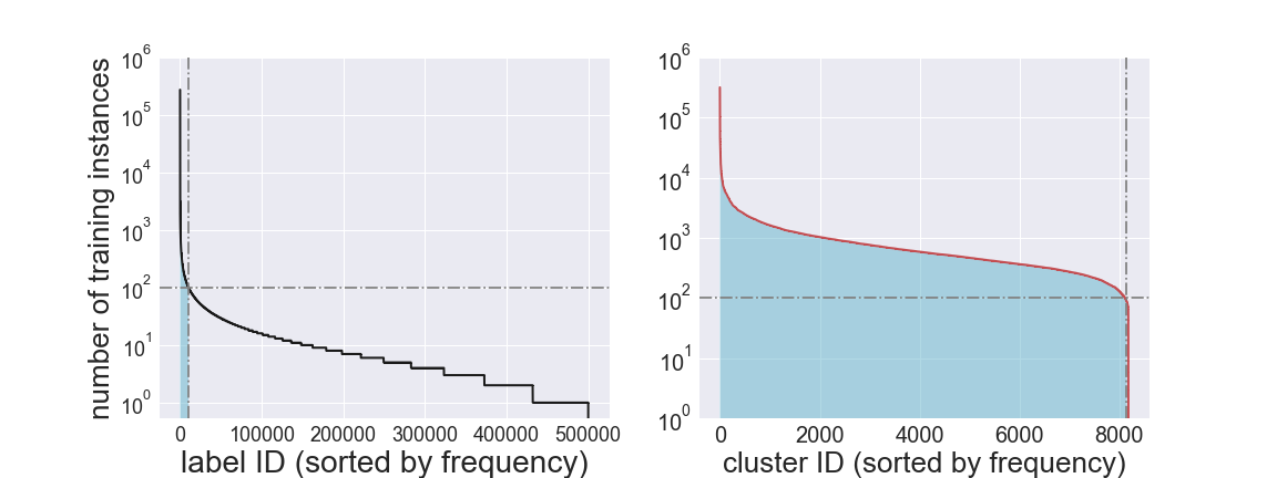
Figure 1: On the left, Wiki-500K shows a long-tail distribution of training data over the labels. Only $2.1\%$ of the labels have more than 100 training instances, as indicated by the cyan blue regime. On the right is the distribution of labels after our semantic label indexing is performed to form 8,192 label clusters; $99.4\%$ of the clusters have more than 100 training instances, which mitigates the data sparsity issue.

Our contributions in this paper are summarized as follows:

• We propose the Prediction for Enormous and Correlated Output Spaces (PECOS) framework, a versatile and modular machine learning framework for solving prediction problems for very large output spaces. The versatility of PECOS comes from our proposed three-phase approach: (i) semantic label indexing, (ii) machine learned matching, and finally (iii) ranking.

• The flexibility of PECOS allows practitioners to evaluate the trade-offs between performance and infrastructure cost to identify the most appropriate PECOS variant for their application.

• To exhibit the flexibility of PECOS, we propose three concrete realizations: (i) XR-LINEAR is a recursive linear machine learned realization of our PECOS framework; (ii) X-TRANSFORMER is a neural realization of the PECOS framework without recursive Transformer encoders; (iii)XR-TRANSFORMER is a neural realization of the PECOS framework with recursive Transformer encoders;

• We present detailed experimental results showing that PECOS yields state-of-the-art results for XMR in terms of precision, recall, and computational time (training and inference).

Parts of this paper related to X-TRANSFORMER and XR-TRANSFORMER have appeared in Chang et al. [7] and  Zhang et al. [54], respectively, while the part related to fast inference has appeared in Etter et al. [13].

This paper is organized as follows: we setup the problem formulation in Section 1.1. In Section 2, we propose a three-phase framework for PECOS and describe each phase in detail. Next, we present XR-LINEAR, a recursive linear machine learned realization in Section 3, and X-TRANSFORMER and XR-TRANSFORMER, the neural realization for inputs in textual form in Section 4. We then discuss the connections of PECOS to related work in Section 5. We present detailed experimental results in Section 6 and conclude our paper in Section 7. The PECOS software is available at https://libpecos.org.

1.1 Setting the Scene

In this paper, we focus on the eXtreme Multilabel Ranking (XMR) problem: given an input instance, return the most relevant labels from an enormous label collection, where the number of labels could be in the millions or more. One can view the XMR problem as learning a score function $f:\mathcal{X}\times\mathcal{Y}\rightarrow\mathds{R}$, that maps an (instance, label) pair $({\bm{x}},\ell)$ to a score $f({\bm{x}},\ell)$, where $\ell\in\mathcal{Y}$. The function $f$ should be optimized such that highly relevant $({\bm{x}},y)$ pairs have high scores, whereas irrelevant pairs have low scores. Many real-world applications are in this form. For example, in E-commerce dynamic search advertising, ${\bm{x}}$ represents an item and $\ell$ represents a bid query on the market [36, 37]. In open-domain question answering, ${\bm{x}}$ represents a question and $\ell$ represents an evidence passage containing the answer [25, 6]. In the PASCAL Large-Scale Hierarchical Text Classification (LSHTC) challenge, ${\bm{x}}$ represents an article and ${\bm{y}}$ represents a category in the hierarchical Wikipedia taxonomy [34].

Formally speaking, in an XMR problem, we are given a training dataset $\mathopen{}\mathclose{{}\left\{{({\bm{x}}_{i},{\bm{y}}_{i}):i=1,\ldots,n}}\right\}$, where ${\bm{x}}_{i}\in\mathds{R}^{d}$ is a $d$-dimensional feature vector for the $i$-th instance, and ${\bm{y}}_{i}\in\mathopen{}\mathclose{{}\left\{{0,1}}\right\}^{L}$ denotes the relevant labels for this instance from an output space $\mathcal{Y}\equiv\mathopen{}\mathclose{{}\left\{{1,\ldots,\ell,\ldots,L}}\right\}$ with $L$ labels. In a typical XMR problem, the number of instances $n$, the number of instance features $d$, and the number of labels $L$ can all be in the millions, or larger. We also use $X=[{\bm{x}}_{1},\ldots,{\bm{x}}_{i},\ldots,{\bm{x}}_{n}]^{\top}\in\mathds{R}^{n\times d}$ to denote the input feature matrix, and use $Y=[{\bm{y}}_{1},\ldots,{\bm{y}}_{i},\ldots,{\bm{y}}_{n}]^{\top}\in\mathopen{}\mathclose{{}\left\{{0,1}}\right\}^{n\times L}$ to denote the input-to-label matrix.

The scoring function $f({\bm{x}},\ell):\mathds{R}^{d}\times\mathcal{Y}\rightarrow\mathds{R}$ is to be learned from the given training data such that $f({\bm{x}},\ell)$ maps an input (or instance) ${\bm{x}}$ and a label $\ell$ to a relevance score, which can be used to identify labels most relevant to ${\bm{x}}$ from the output space $\mathcal{Y}$. Since the top scores are the salient ones, we further use $f_{b}({\bm{x}})\subset\mathcal{Y}$ to denote the top-$b$ predicted labels for a given instance ${\bm{x}}$, i.e.,

$$f_{b}({\bm{x}})=\mathop{\arg\max}_{\mathcal{S}\subset\mathcal{Y}:\mathopen{}\mathclose{{}\left|{\mathcal{S}}}\right|=b}\sum_{\ell\in\mathcal{S}}f({\bm{x}},\ell).$$

To evaluate the feasibility of $f(\cdot)$ for a given XMR problem, we need to consider the following questions:

• Quality of $f_{b}(\cdot)$: how well does $f_{b}(\cdot)$ perform on an unseen input instance ${\bm{x}}$?

• Training Efficiency: how efficient is the training algorithm in learning the parameters of $f(\cdot)$?

• Inference Speed: how fast is the computation of $f_{b}(\cdot)$ to serve real-time requests?

• Infrastructure Cost: how much do the training and inference procedures cost in terms of computational resources?

As an example, using the vanilla linear one-versus-rest (OVR) approach [5], the scoring function can be defined on each label as follows:

$$f({\bm{x}},\ell)={\bm{w}}_{\ell}^{\top}{\bm{x}},\ \forall\ell\in\mathcal{Y}.$$ (1)

The parameter ${\bm{w}}_{\ell}\in\mathds{R}^{d}$ for the $\ell$-th label may be obtained by solving a regularized binary classification problem:

$${\bm{w}}_{\ell}=\arg\max_{{\bm{w}}\in\mathds{R}^{d}}\sum_{i=1}^{n}\mathcal{L}(Y_{i\ell},{\bm{w}}^{\top}{\bm{x}}_{i})+\frac{\lambda}{2}{\bm{w}}^{\top}{\bm{w}},$$ (2)

where $\mathcal{L}(\cdot,\cdot)$ is a loss function and $\lambda>0$ is a regularization hyperparameter. The overall parameter space for this linear OVR approach is $\mathcal{O}(dL)$, the training time is $L\times T_{\text{binary}}$, and the inference time is $\Omega(dL)$, where $T_{\text{binary}}$ is the time required to train a binary classifier. Usually, $T_{\text{binary}}$ is at least linear in the number of nonzeros in the training data, which we denote by $\text{nnz}(X)$.

Let us sketch a ballpark estimate of how long it would take to train an OVR model on the Wiki-500K dataset with $n=$ 1.5 million text training documents and $L=$ 0.5 million output labels, with average number of tokens in each document being around $1,000$. Further suppose that we use logistic regression as our binary classifier and the term frequency-inverse document frequency (tfidf) vectorizer with a vocabulary of size 2.5 million to form a sparse training matrix $X\in\mathds{R}^{1.5\cdot 10^{6}\times 2.5\cdot 10^{6}}$. With such a training matrix $X$ each logistic regression can be trained in about 50 seconds [14, 16]. Note that the training time remains similar even if we use dense embeddings to form a dense feature matrix $X$ as $\text{nnz}(X)$ might be even larger than the sparse tfidf feature matrix. In this setting, the overall training time will be around $1.5\cdot 10^{6}\times 50=7.5\cdot 10^{7}\text{ seconds }=\frac{7.5\cdot 10^{7}}{\mathopen{}\mathclose{{}\left({60\times 60\times 24\times 30}}\right)}\approx 29\;\text{months}$ on 1 CPU and 1.8 months even with perfect 16-way parallelization! Further, the full model would require a prohibitive amount of $2.5\cdot 10^{6}\times 0.5\cdot 10^{6}\times 4\;\text{Bytes}\approx$ $5$ TB disk space (assuming a single precision floating point format). Clearly such a simple approach is not feasible for an XMR problem of this scale even with linear models. Note that the simple deep learning extension to multi-label classification (e.g., binary cross entry or softmax losses), which jointly learns parameters for all labels, only imposes more computational requirements. Another important aspect is that the inference for the OVR approach is extremely slow when $L$ is large as the inference time has $\mathcal{O}(L)$ complexity. Clearly, both training and inference times and memory are prohibitive for a simple OVR solution. In contrast, with PECOS, we are able to train a dataset of this size ($n=1.5\cdot 10^{6}$, $d=2.5\cdot 10^{6}$, $L=0.5\cdot 10^{6}$) in 5 hours on a 16 CPU machine with the model requiring about 5 GB space. This PECOS model also allows inference in $\mathcal{O}(\log L)$ time.

2 PECOS XMR Framework

In order to build a framework to solve general XMR problems, we borrow from the design of modern information retrieval (IR) systems where the goal is to find the top few relevant documents for a given query from an extremely large number of documents. IR can be regarded as a special XMR problem with queries as inputs and documents as output labels. Furthermore, when both queries and documents are in the same text domain, an efficient and scalable IR system such as Apache Lucene, typically consists of the following stages [15]; 1) lexical indexing: building an efficient data structure in an offline manner to lexically index the documents by its tokens; 2) lexical matching: finding the documents that contain this query; and 3) ranking: scoring the matched documents, often using machine learning. This three stage design is crucial to any scalable IR system that deals with a large number of documents.

Albeit scalable, an IR system cannot be easily generalized to handle general XMR problems due to the following reasons. First, output labels for a general XMR problem might not have text information so the lexical indexing approach is not applicable. Second, input instances and output labels for a general XMR problem might not be in the same domain, for example, the inputs could be images and the labels could be image annotations. Third, input instances for a general XMR problem are usually in a feature vector form instead of in text form, so the indexing/matching techniques in IR are not applicable.

Motivated by the design for IR systems, in PECOS, we propose a three-stage framework to solve general XMR problems in a scalable and modular manner:

• Semantic Label Indexing: we organize the original label space $\mathcal{Y}$, $\mathopen{}\mathclose{{}\left|{\mathcal{Y}}}\right|=L$, so that semantically similar labels are arranged together. One way is to partition the labels into $K$ clusters, $\mathopen{}\mathclose{{}\left\{{\mathcal{Y}_{k}:k=1,\ldots,K}}\right\}$, where $K\ll L$ and each cluster $\mathcal{Y}_{k}$ is a subset of labels which are “semantically similar” to each other. Similar to lexical indexing in IR, semantic label indexing is constructed in an offline manner before the training is done. Alternatives for semantic indexing are an approximate kNN index structure.

• Machine-learned Matching: we learn a scoring function $g({\bm{x}},k)$ that maps an input ${\bm{x}}$ to relevant indices/clusters denoted by an indicator vector $\hat{{\bm{m}}}\in\mathopen{}\mathclose{{}\left\{{0,1}}\right\}^{K}$, where the $k$-th element $\hat{m}_{k}=1$ denotes that the $k$-th index/cluster is deemed to be relevant for the input ${\bm{x}}$.

• Ranking: we train a ranker $h({\bm{x}},\ell)$ to give final scores of candidate labels shortlisted by the matcher (given by $\bigcup\limits_{k:\hat{m}_{k}=1}\mathcal{Y}_{k}$). The efficiency of the method stems from only ranking $\mathcal{O}(K)$ ($\ll L$) labels.

With this three-stage framework, the inference complexity can be greatly reduced. For a given input ${\bm{x}}$, let $b=\operatorname{nnz}\mathopen{}\mathclose{{}\left({\hat{{\bm{m}}}}}\right)$ be the number of matched indices/clusters given by $g({\bm{x}},k)$ and let $\text{avg}\mathopen{}\mathclose{{}\left({\mathopen{}\mathclose{{}\left|{\mathcal{Y}_{k}}}\right|}}\right)=L/K$ be the average number of labels in each index/cluster. The inference complexity is reduced to

$$\underbrace{K\times\mathcal{O}(\text{time to evaluate }g({\bm{x}},k))}_{\text{matcher time}}+\underbrace{b\times\frac{L}{K}\times\mathcal{O}(\text{time to evaluate }h({\bm{x}},\ell))}_{\text{ranker time}}.$$

With an appropriate choice of $K$ and $b$, the overall inference time complexity can be drastically reduced. For example, assuming linear models that have time complexity $\mathcal{O}(d)$ for both $g({\bm{x}},k)$ and $h({\bm{x}},\ell)$, if $K=\sqrt{L}$, the time complexity for inference is reduced to $\mathcal{O}(b\times\sqrt{L}\times d)$ from $\mathcal{O}(L\times d)$, which is the time complexity of inference for a vanilla linear OVR model. Later in Section 3, we will show that this time complexity can be further reduced to $\mathcal{O}(b\times\log L\times d)$ by a recursive approach.

It is worthwhile to mention that this framework also alleviates the data sparsity issue that is a major issue in XMR problems. By using clustering for semantic label indexing, tail labels (i.e., labels with fewer positive instances) are clustered with head labels (i.e., labels with more positive instances). This allows the information from head labels to be “transferred” to tail labels using our approach. As a result, most indices (or clusters) contain more positive instances. For example, the right panel of Figure 1 shows the number of positive instances for each index/cluster after semantic label indexing with $K=8,192$ clusters for an XMR dataset with $L=500,000$ labels. We can see that $99.4\%$ of the clusters contain more than $100$ training instances.

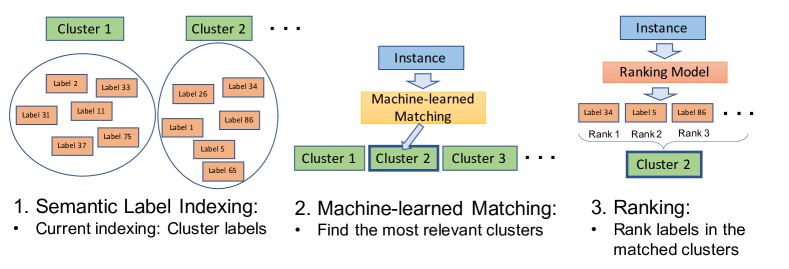
Figure 2: Illustration of the three-stage PECOS framework for XMR.

We now discuss each of the semantic indexing, matching and ranking phases in greater detail.

2.1 Semantic Label Indexing

Inducing label clustering with semantic meaning brings several advantages to our framework. The number of clusters $K$ is typically set to be much smaller than the original label space $L$. Our machine learned matcher $g({\bm{x}},k)$ then needs to map the input to a cluster, which itself is an induced XMR sub-problem where the output space is of size $K$. This significantly reduces computational cost and mitigates the data sparsity issue illustrated in Figure 1. Furthermore, label clustering also plays a crucial role in the learning of the ranker $h({\bm{x}},\ell)$. For example, only labels within a cluster are used to construct “hard” negative instances for training the ranker (more details are in Section 2.3). During inference, ranking is only performed for labels within the top-$b$ clusters predicted by our machine learned matcher $g({\bm{x}},k)$. In some XMR applications, labels may come with some meta information, such as taxonomy or category information which can be used to naturally form a semantic label clustering. However, when such information is not explicitly available, we need to think about how to effectively perform semantic label indexing.

There are two key components to achieve a good semantic label indexing: label representations and indexing/clustering algorithms.

2.1.1 Label Representations

In general, label representations or label embeddings should encode the semantic information such that two labels with high semantic similarity have a high chance to be grouped together. We use $\mathopen{}\mathclose{{}\left\{{{\bm{z}}_{\ell}:\ell\in\mathcal{Y}}}\right\}$ to denote the label representations. If meta information is available for labels, we can construct label representations directly from that information. For example, if labels come with meaningful text descriptions such as the category information for Wiki pages, we can use either traditional approaches such as term frequency-inverse document frequency (tfidf) or recent deep-learning based text embedding approaches such as Word2Vec [31], ELMo [35] to form label representations. If labels come with a graph structure such as co-purchase graphs among items or friendship among users, one can consider forming graph Laplacians [40] or graph convolution neural networks [48] to obtain label representations. Here, we present a few alternative ways to represent labels when such meta information is not available.

Label Representation via Positive Instance Indices (PII). PII is a simple approach to represent each label by the membership of its instances:

$${\bm{z}}_{\ell}^{\text{{\sf PII}}}:=\frac{\bar{{\bm{y}}}_{\ell}}{\mathopen{}\mathclose{{}\left\|{\bar{{\bm{y}}}_{\ell}}}\right\|},\quad\ell\in\mathcal{Y},$$

where $\bar{{\bm{y}}}_{\ell}\in\mathopen{}\mathclose{{}\left\{{0,1}}\right\}^{n}$ is the $\ell$-th column of the instance-to-label matrix $Y$.

Label Representation via Positive Instance Feature Aggregation (PIFA). In PIFA, each label is represented by aggregating feature vectors from positive instances:

$${\bm{z}}_{\ell}^{\text{{\sf PIFA}}} =\frac{{\bm{v}}_{\ell}}{\mathopen{}\mathclose{{}\left\|{{\bm{v}}_{\ell}}}\right\|},\text{ where }\ {\bm{v}}_{\ell}=\sum_{i=1}^{L}Y_{i\ell}{\bm{x}}_{i}=\mathopen{}\mathclose{{}\left({X^{\top}Y}}\right)_{\ell},\quad\ell\in\mathcal{Y},$$

where ${\bm{x}}_{i}$ is the feature representation of the $i$-th training instance, and $X=\mathopen{}\mathclose{{}\left[{{\bm{x}}_{1},\ldots,{\bm{x}}_{i},\ldots,{\bm{x}}_{n}}}\right]^{\top}$ is the training instance matrix. Note that the dimension of PIFA representations is $d$, which is different from the dimension of PII representations $n$.

Label Representation via Label Features in addition to PIFA (PIFA + LF). If a label feature matrix $\tilde{Z}=[\tilde{{\bm{z}}}_{1},\ldots,\tilde{{\bm{z}}}_{\ell},\ldots,\tilde{{\bm{z}}}_{L}]^{\top}\in\mathds{R}^{d\times L}$ is given and $\tilde{{\bm{z}}}_{\ell}$ and ${\bm{x}}_{i}$ are in the same domain, we can consider a weighted combination of $\tilde{{\bm{z}}}_{\ell}$ and PIFA representation as follows:

$${\bm{z}}_{\ell}^{\text{{\sf PIFA} + {\sf LF}}}=(1-\alpha_{\ell})\tilde{{\bm{z}}}_{\ell}+\alpha_{\ell}{\bm{z}}_{\ell}^{\text{{\sf PIFA}}}=\mathopen{}\mathclose{{}\left({(1-\alpha_{\ell})\tilde{Z}+\alpha_{\ell}\mathopen{}\mathclose{{}\left({X^{\top}Y}}\right)}}\right)_{\ell}.$$

Label Representation via Graph Spectrum (Spectral). In Spectral, we consider the instance-to-label matrix $Y$ as a bi-partite graph between instances and labels. We can then follow the co-clustering algorithm described in Dhillon [10] to obtain spectral representations for labels. In particular, we first form a normalized label matrix $\tilde{Y}$ as follows

$$\tilde{Y}=D_{1}^{-1/2}YD_{2}^{-1/2},$$

where $D_{1}\in\mathds{R}^{n\times n}$, and $D_{2}\in\mathds{R}^{L\times L}$ are degree diagonal matrices such that $(D_{1})_{ii}=\sum_{\ell}Y_{i\ell}$ and $(D_{2})_{\ell\ell}=\sum_{i}Y_{i\ell}$. Next, let $\mathopen{}\mathclose{{}\left\{{({\bm{u}}_{t},{\bm{v}}_{t}):{\bm{u}}_{t}\in\mathds{R}^{n},\ {\bm{v}}_{t}\in\mathds{R}^{L},\ t=2,\ldots,k+1}}\right\}$ be the singular vector pairs (left and right) corresponding to the 2nd,$\ldots$, $k+1$-st largest singular values of $\tilde{Y}$. Following Dhillon [10, Eq. 12], we can construct a $k$-dimensional label representation matrix as follows:

$${\bm{z}}_{\ell}^{\text{{\sf Spectral}}} =\text{the $\ell$-th row of $Z$},\quad Z=D_{2}^{-1/2}[{\bm{v}}_{2},\ldots,{\bm{v}}_{k+1}]^{\top}\in\mathds{R}^{L\times k}.$$

See Figure 3 for an illustration of the indexing matrix with $L=9$ labels and $K=3$ clusters.

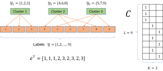
Figure 3: Illustration of Label Indexing/Clustering. ${\bm{c}}\in\mathopen{}\mathclose{{}\left\{{1,2,3}}\right\}^{9}$ denotes the clustering vector with $c_{\ell}$ being the index of the cluster containing the $\ell$-th label, while $C\in\mathopen{}\mathclose{{}\left\{{0,1}}\right\}^{9\times 3}$ denotes the cluster indicator matrix (with same information as ${\bm{c}}$).

2.1.2 Semantic Indexing Through Clustering

Once the label representations $\mathopen{}\mathclose{{}\left\{{{\bm{z}}_{\ell}:\ell\in\mathcal{Y}}}\right\}$ are decided, we can get a semantic indexing scheme using an appropriate clustering. Let $\mathcal{C}=\mathopen{}\mathclose{{}\left\{{1,\ldots,K}}\right\}$ denote the set of $K$ label clusters. The purpose of our clustering algorithm is to learn a label-to-cluster assignment: ${\bm{c}}\in\mathcal{C}^{L}$, where $c_{\ell}$ denotes the index of the cluster containing the label $\ell$. Equivalently, the clustering assignment can also be represented by the indexing matrix $C\in\mathopen{}\mathclose{{}\left\{{0,1}}\right\}^{L\times K}$ as follows:

$$C_{lk} =\begin{cases}1,&\text{ if }k=c_{\ell},\\ 0,&\text{ otherwise.}\end{cases}$$ (3)

Below we give the objective used in two popular $K$-Means [12] and Spherical $K$-Means [11] clustering algorithms:

$${\bm{c}}^{\text{K-MEANS}}= \arg\min_{{\bm{c}}\in\mathcal{C}^{L}}\quad\sum_{k\in\mathcal{C}}\sum_{\ell:c_{\ell}=k}\mathopen{}\mathclose{{}\left\|{{\bm{z}}_{\ell}-\mathbf{\bm{\mu}}_{k}}}\right\|^{2},\quad\text{where}\ \mathbf{\bm{\mu}}_{k}:=\frac{\sum_{\ell:c_{\ell}=k}{\bm{z}}_{\ell}}{\mathopen{}\mathclose{{}\left|{\mathopen{}\mathclose{{}\left\{{l:c_{\ell}=k}}\right\}}}\right|},$$ (4)

$${\bm{c}}^{\text{SK-MEANS}}= \arg\max_{{\bm{c}}\in\mathcal{C}^{L}}\quad\sum_{k\in\mathcal{C}}\sum_{\ell:c_{\ell}=k}\frac{{\bm{z}}_{\ell}^{\top}\mathbf{\bm{\mu}}_{k}}{\mathopen{}\mathclose{{}\left\|{{\bm{z}}_{\ell}}}\right\|\mathopen{}\mathclose{{}\left\|{\mathbf{\bm{\mu}}_{k}}}\right\|},\quad\text{where}\ \mathbf{\bm{\mu}}_{k}:=\frac{\sum_{l:c_{\ell}=k}{\bm{z}}_{\ell}}{\mathopen{}\mathclose{{}\left\|{\sum_{\ell:c_{\ell}=k}{\bm{z}}_{\ell}}}\right\|}.$$ (5)

Standard $K$-Means/Spherical $K$-Means algorithms have $\mathcal{O}(\operatorname{nnz}(Z)\times K\times\text{\# iterations})$ computation complexity, where $Z$ is the label representation matrix. This can still be very time consuming if $K$ is also large (say $K=10^{4}$). In PECOS, we provide an implementation which utilizes a recursive $B$-ary partitioning approach to further improve the efficiency of label clustering, see Algorithm 1 The high level idea is to apply $B$-ary partitioning on the label set by either $B$-Means or spherical $B$-Means recursively. $B$ is usually chosen as a small constant such as $2$ or $16$. An illustration with $B=2$ is given in Figure 4. The time complexity of Algorithm 1 is $\mathcal{O}(\operatorname{nnz}(Z)\times\log_{B}K\times\text{\# iterations})$, which is much lower than directly clustering into $K$ clusters, which would have time complexity that is linear in $K$.

Algorithm 1 Clustering with $B$-ary partitions Input: — $\mathcal{Y}$: label indices and $\mathopen{}\mathclose{{}\left\{{{\bm{z}}_{\ell}:\ell\in\mathcal{Y}}}\right\}$ representations, — $K=B^{D-1}$: number of clusters. Output: indexing matrix: $C\in\mathopen{}\mathclose{{}\left\{{0,1}}\right\}^{L\times K}$ • $\mathcal{Y}^{(1)}_{1}\leftarrow\mathcal{Y}$ • For $t=1,\ldots,D$ — For $k=1,\ldots,B^{t-1}$ compactitemiii perform either $B$-Means or Spherical $B$-Means to partition $\mathcal{Y}^{(t)}_{k}$ into $B$ clusters $\mathopen{}\mathclose{{}\left\{{\mathcal{Y}^{(t+1)}_{B(k-1)+j}:j=1,\ldots,B}}\right\}$ • construct $C$ with $C_{lk}=\begin{cases}1&\text{ if }\ell\in\mathcal{Y}^{(D+1)}_{k},\\ 0&\text{ otherwise.}\end{cases}$ Figure 4: Illustration of label clustering with recursive $B$-ary partitions with $B=2$.

2.1.3 Other Indexing Methods

In this paper, we mainly focus on label clustering as the algorithmic choice for the semantic label indexing phase. There are other strategies which might be promising alternatives for PECOS, which we leave as direction for future exploration. When using typical clustering algorithms like $K$-Means each label is assigned to exactly one label cluster. However, labels in real world applications might have more than one semantic meaning. For example, “apple” could be either a fruit or a brand. Thus, one interesting direction to explore is to adopt overlapping clustering algorithms such as Whang et al. [46] for semantic label indexing. Recently, Liu et al. [28] propose to find overlapped clusters by jointly optimizing cluster assignments and model parameters of partition-based XMR models, which is complementary to our PECOS framework.

In addition, we can use various approximate nearest neighbor (ANN) search [26] schemes as the basis of semantic indexing. There is a successful attempt by Jain et al. [18] to apply a state-of-the-art approx ANN search algorithm called hierarchical navigable small world (HNSW) graphs [30] for the XMR problem when the feature vectors are low-dimensional dense embeddings. The ability of variants of the HNSW data structure such as Rand-NSG [41] to quickly get a small match set for any given input would be very suitable for the three-stage design framework of PECOS.

2.2 Machine Learned Matching

The matching stage in PECOS is crucial since the final ranking stage is restricted to the labels returned by the matcher; hence if the matcher fails to identify the candidate labels accurately, performance can greatly suffer. In general, the input features ${\bm{x}}_{i}$ and label representations ${\bm{z}}_{\ell}$ could be in different domains and have different dimensionalities. Thus, in the machine learned matching stage, we need to learn a general matcher function $g({\bm{x}},k)$ which finds the relevance between a given instance ${\bm{x}}$ and the $k$-th label cluster. This matching scoring function can then be used to obtain the top-$b$ label clusters:

$$g_{b}({\bm{x}})=\mathop{\arg\max}_{\mathcal{S}\subset\mathcal{C}:\mathopen{}\mathclose{{}\left|{\mathcal{S}}}\right|=b}\sum_{k\in\mathcal{S}}g({\bm{x}},k).$$

Given a semantic label indexing denoted by the clustering matrix $C\in\mathopen{}\mathclose{{}\left\{{0,1}}\right\}^{L\times K}$, the original XMR problem with the output space $\mathcal{Y}$ morphs to an XMR sub-problem with a much smaller output space $\mathcal{C}$ of size $K$. In particular, we can transform the original training dataset $\mathopen{}\mathclose{{}\left\{{({\bm{x}}_{i},{\bm{y}}_{i}):i=1,\ldots,n}}\right\}$ to a new dataset $\mathopen{}\mathclose{{}\left\{{({\bm{x}}_{i},{\bm{m}}_{i}):i=1,\ldots,n}}\right\}$, where ${\bm{m}}_{i}\in\mathopen{}\mathclose{{}\left\{{0,1}}\right\}^{K}=\text{binarize}\mathopen{}\mathclose{{}\left({C^{\top}{\bm{y}}_{i}}}\right)$ denotes the ground truth input-to-cluster assignment for the $i$-th training instance. Similar to the instance-to-label matrix $Y$, we can stack the ground truth $\mathopen{}\mathclose{{}\left\{{{\bm{m}}_{i}}}\right\}$ into the ground truth input-to-cluster assignment matrix $M=[{\bm{m}}_{1},\ldots,{\bm{m}}_{i},\ldots,{\bm{m}}_{n}]^{\top}\in\mathopen{}\mathclose{{}\left\{{0,1}}\right\}^{n\times K}$. For any given indexing matrix $C$, the ground truth $M$ can be obtained by

$$M=\text{binarize}(\tilde{M}),\text{ where }\ \tilde{M}=YC,$$

where $M_{ik}=\operatorname{\mathds{I}}\mathopen{}\mathclose{{}\left[\sum_{\ell\in\mathcal{Y}}Y_{i\ell}C_{lk}>0}\right]$. Note that if we wanted a weighted input-to-cluster matrix, we could work with $\tilde{M}$ instead.

Thus, the machine learned matcher reduces to an XMR problem with a smaller output space of size $K$. Hence, we can apply any existing multi-label classifier which can handle $K$ labels. For example, if $K$ is not very large, we can consider the aforementioned vanilla one-versus-rest (OVR) approach to learn the matcher $g({\bm{x}},k)$. If $K$ is still too large, we can recursively apply the three-stage PECOS framework to learn the matcher. We will give an example of this recursive PECOS approach, called XR-LINEAR, in Section 3.

Note that if the cluster of a relevant label is not correctly predicted by the matcher, this relevant label does not have a chance to be surfaced by our ranker at all. Thus, in Section 4, we consider using more advanced deep learning based approaches to learn the matcher, especially when the input instances are in text form.

2.3 Ranking

The goal of the ranker $h({\bm{x}},\ell)$ is to model the relevance between the input ${\bm{x}}$ and the shortlisted labels obtained from the relevant label clusters identified by our matcher $g_{b}({\bm{x}})$. Informally, the shortlist of candidate labels is the set of label clusters. Given a label-to-cluster assignment vector ${\bm{c}}\in\mathopen{}\mathclose{{}\left\{{1,\ldots,K}}\right\}^{L}$, where the $k$-th cluster is given by $\mathcal{Y}_{k}=\mathopen{}\mathclose{{}\left\{{\ell\in\mathcal{Y}:c_{\ell}=k}}\right\}$, the “shortlisting” operation for an input ${\bm{x}}$ can be formally described by $s(\bar{{\bm{m}}}|{\bm{c}})$ as follows:

$$s(\bar{{\bm{m}}}|{\bm{c}}) =\bigcup\limits_{k:\bar{m}_{k}\neq 0}\mathcal{Y}_{k},$$ (6)

where $\bar{{\bm{m}}}\in\mathopen{}\mathclose{{}\left\{{0,1}}\right\}^{K}$ is the cluster indicator vector for the input ${\bm{x}}$. Here $\bar{m}_{k}=1$ denotes that the $k$-th cluster is considered relevant to the input ${\bm{x}}$. In general, for the $i$-th input ${\bm{x}}_{i}$, this indicator vector $\bar{{\bm{m}}}_{i}$ can come from either the ground truth input-to-cluster assignment $\mathopen{}\mathclose{{}\left\{{{\bm{m}}_{i}}}\right\}$ defined in Section 2.2 or the relevant clusters predicted by our machine learned matcher $\mathopen{}\mathclose{{}\left\{{\hat{{\bm{m}}}_{i}}}\right\}$, where the details are provided in Section 2.3.1. Note that, given the clustering, ${\bm{m}}_{i}$ is an induced static assignment while the choice of $\hat{{\bm{m}}}_{i}$ from the machine learned matcher depends on the predictions made by the matcher. In particular, we use $\hat{{\bm{m}}}$ to denote the indicator vector of label clusters predicted by our matcher $g_{b}({\bm{x}})$:

$$\hat{m}_{k}=\begin{cases}1&\text{ if }k\in g_{b}({\bm{x}}),\\ 0&\text{ otherwise. }\end{cases}$$

The ideal ranker $h({\bm{x}},\ell)$ for the given matcher $g_{b}({\bm{x}})$ should satisfy the property:

$$h({\bm{x}},\ell_{1})>h({\bm{x}},\ell_{2})\Leftrightarrow\ell_{1}\succ_{{\bm{x}}}\ell_{2}\quad\forall\ell_{1},\ell_{2}\in s(\hat{{\bm{m}}}|{\bm{c}}),$$ (7)

where $\ell_{1}\succ_{{\bm{x}}}\ell_{2}$ denotes that label $\ell_{1}$ is more relevant than label $\ell_{2}$ for the input ${\bm{x}}$ in the ordering of the ground truth.

In general, one can choose any ML ranking model as the ranker. Common choices include linear models, gradient boosting decision trees (GBDT) and neural nets. Choices of the loss function include point-wise, pair-wise, and list-wise ranking losses. The modeling of PECOS allows for easy inclusion of various rankers.

2.3.1 Hard Negative Sampling for Ranker Training in PECOS

One of the key components in learning a ranking model is to identify the sets of positive (relevant) and negative (irrelevant) labels for each instance. Unlike most standard ranking problems where positive and negative labels for each instance are explicitly provided in the training dataset, for each instance in an XMR problem, we are usually provided a small number of explicit relevant labels and abundant implicit irrelevant labels. Obviously, including all implicit irrelevant labels as negative labels to train a ranker is not feasible as it greatly increases training time with little increase in accuracy. Hence, we propose to include only hard negatives, by restricting them to be irrelevant labels from relevant label clusters for each instance. In particular, for a given instance ${\bm{x}}_{i}$, letting $\bar{{\bm{m}}}_{i}$ be the indicator vector for the relevant clusters, we have

$$\text{positives}({\bm{x}}_{i}) =\mathopen{}\mathclose{{}\left\{{\ell\in s(\bar{{\bm{m}}}_{i}|{\bm{c}}):Y_{i\ell}=1}}\right\},$$

$$\text{negatives}({\bm{x}}_{i}) =\mathopen{}\mathclose{{}\left\{{\ell\in s(\bar{{\bm{m}}}_{i}|{\bm{c}}):Y_{i\ell}\neq 1}}\right\},$$ (8)

where $s(\bar{{\bm{m}}}_{i}|{\bm{c}})$ is as in (6), and gives the shortlist candidate set of labels for training instance ${\bm{x}}_{i}$.

Depending on the choice of the indicator vectors $\mathopen{}\mathclose{{}\left\{{\bar{{\bm{m}}}_{i}}}\right\}$, we have the following hard negative sampling schemes.

Teacher Forcing Negatives (TFN). Teacher forcing [47, 24] is a known training strategy used in recurrent neural networks (RNN), where the ground truth for earlier outputs is fed back into RNN training to be conditioned on for the prediction of later outputs. In our framework, we use teacher forcing negatives (TFN) to denote the hard negative sampling scheme where the ground-truth input-to-cluster assignment for the input ${\bm{x}}_{i}$ is used to identify hard negative labels for the training of the ranker. In particular, the input-to-cluster assignment is chosen as follows:

$$\bar{{\bm{m}}}_{i}\leftarrow{\bm{m}}_{i},\ \forall i,$$

where ${\bm{m}}_{i}$ is the ground-truth input-to-cluster assigned used to train our matcher in Section 2.2. As discovered in Bengio et al. [3], the teacher forcing scheme can lead to a discrepancy between training and inference for recurrent models. In particular, during inference, the unknown ground truth is replaced by the prediction generated by the model itself. This discrepancy leads to sub-optimal performance for the models trained with the teacher forcing strategy. Similarly, this discrepancy also appears in the TFN sampling scheme for inferring our hard negatives as ${\bm{m}}_{i}$ is independent of the performance of our matcher.

Matcher Aware Negatives (MAN). An alternative strategy is to include matcher-aware hard negatives for each training instance. In particular, for each input ${\bm{x}}_{i}$, we can use the instance-to-cluster indicator $\hat{{\bm{m}}}_{i}$ predicted by our matcher:

$$\bar{{\bm{m}}}_{i}\leftarrow\hat{{\bm{m}}}_{i},\ \forall i.$$

In practice, we observe that a union of TFN and MAN yields the best performance:

$$\bar{{\bm{m}}}_{i}\leftarrow\text{binarize}\mathopen{}\mathclose{{}\left({{\bm{m}}_{i}+\hat{{\bm{m}}}_{i}}}\right),\ \forall i.$$

See Figure 5 for an illustration of how to identify the set of shortlisted labels in order to train the OVR classifier for each label, given an input-to-cluster indicator vector $\bar{{\bm{m}}}_{i}$.

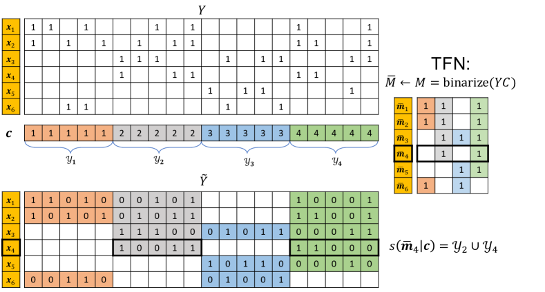
Figure 5: Illustration of Hard Negative Sampling for Ranker Training in PECOS. In this toy XMR example, we have $n=6$ instances, $L=20$ labels, and $K=4$ label clusters. $Y$ shown on the top, denotes the ground-truth input-to-label matrix where explicit positives are denoted by $1$. ${\bm{c}}\in\mathopen{}\mathclose{{}\left\{{1,\ldots,4}}\right\}^{20}$ is the label-to-cluster assignment vector for the label clustering $\mathopen{}\mathclose{{}\left\{{\mathcal{Y}_{k}:k=1,\ldots,4}}\right\}$. We illustrate how to identify the set of shortlisted labels given a input-to-cluster indicator vector ${\bm{m}}_{i}$. (TFN chooses $\bar{M}$ to be $M$: $\bar{M}\leftarrow M=[\cdots{\bm{m}}_{i}\cdots]^{\top}$ is the matrix obtained by stacking $\mathopen{}\mathclose{{}\left\{{{\bm{m}}_{i}}}\right\}$). Taking ${\bm{x}}_{4}$ as an example, the positive labels are ${\bm{y}}_{4}^{+}=\mathopen{}\mathclose{{}\left\{{6,9,10,16,17}}\right\}$. $\bar{{\bm{m}}}_{4}$ is an example instance-to-cluster indicator where only the second and the fourth clusters are chosen: ${\bm{m}}_{4}\leftarrow[0,1,0,1]^{\top}$. As a result, only labels from the shortlisted candidates $s(\bar{{\bm{m}}}_{4}|{\bm{c}})=\mathcal{Y}_{2}\cup\mathcal{Y}_{4}=\mathopen{}\mathclose{{}\left\{{6,7,8,9,10,16,17,18,19,20}}\right\}$ are considered in the training of the ranker for instance ${\bm{x}}_{4}$. In particular, the negative labels for ${\bm{x}}_{4}$, denoted by cells with explicit zeros on the bottom, become $s(\bar{{\bm{m}}}_{4}|{\bm{c}})\setminus{\bm{y}}_{4}^{+}=\mathopen{}\mathclose{{}\left\{{7,8,18,19,20}}\right\}$ instead of $\mathcal{Y}\setminus{\bm{y}}_{4}^{+}$. The choice of $\bar{M}$ in above example follows teacher forcing negatives (TFN): $\bar{M}\leftarrow M$ (i.e., $\bar{{\bm{m}}}_{i}\leftarrow{\bm{m}}_{i},\ \forall i$), which denotes that the ground-truth input-to-cluster indicator ${\bm{m}}_{i}=\text{binarize}(C^{\top}{\bm{y}}_{i})$ is used to induce hard negatives for each input. See Section 2.3.1 for more discussion about various hard negative sampling schemes.

2.3.2 A One-Versus-Rest Linear Ranker

In general, we can use any ranker with a corresponding ranking loss function in PECOS. Here we present a simple one-versus-rest linear ranker with a point-wise ranking loss. In particular, the linear ranker is parametrized by a matrix $W=[{\bm{w}}_{1},\ldots,{\bm{w}}_{\ell},\ldots,{\bm{w}}_{L}]\in\mathds{R}^{d\times L}$ of parameters as follows.

$$h({\bm{x}},\ell)={\bm{w}}_{\ell}^{\top}{\bm{x}}_{i},\quad\ell\in\mathcal{Y}.$$

Given an indexing vector ${\bm{c}}$ and an instance-to-cluster matrix $\bar{M}$, the parameters $W$ can be obtained by solving the following optimization problem:

$$\min_{W}\quad \sum_{i=1}^{n}\sum_{\ell\in s(\bar{{\bm{m}}}_{i}|{\bm{c}})}\mathcal{L}(Y_{i\ell},{\bm{w}}_{\ell}^{\top}{\bm{x}}_{i})+\frac{\lambda}{2}\sum_{\ell=1}^{L}\mathopen{}\mathclose{{}\left\|{{\bm{w}}_{\ell}}}\right\|^{2},$$ (9)

where $\mathcal{L}(\cdot,\cdot)$ is a point-wise loss function such as

$$\mathcal{L}_{\text{hinge}}(y,h) =\max\mathopen{}\mathclose{{}\left\{{0,1-\dot{y}h}}\right\},$$

$$\mathcal{L}_{\text{squared-hinge}}(y,h) =\max\mathopen{}\mathclose{{}\left\{{0,1-\dot{y}h}}\right\}^{2},$$

$$\mathcal{L}_{\text{logistic}}(y,h) =\log\mathopen{}\mathclose{{}\left\{{1+\exp\mathopen{}\mathclose{{}\left({-\dot{y}h}}\right)}}\right\},$$

where $\dot{y}=2y-1$, which maps $y$ from $\mathopen{}\mathclose{{}\left\{{0,1}}\right\}$ to $\mathopen{}\mathclose{{}\left\{{-1,+1}}\right\}$. Due to the choice of point-wise loss, (9) can be decomposed into $L$ independent binary classification problems as follows.

$$\min_{W}\quad\sum_{i=1}^{n}\sum_{\ell\in s(\bar{{\bm{m}}}_{i}|{\bm{c}})}\mathcal{L}(Y_{i\ell},{\bm{w}}_{\ell}^{\top}{\bm{x}}_{i})+\frac{\lambda}{2}\sum_{\ell=1}^{L}\mathopen{}\mathclose{{}\left\|{{\bm{w}}_{\ell}}}\right\|^{2}$$

$$= \quad\min_{W}\ \sum_{\ell\in\mathcal{Y}}\mathopen{}\mathclose{{}\left\{{\sum_{i:\bar{M}_{ic_{\ell}}\neq 0}\mathcal{L}(Y_{i\ell},{\bm{w}}_{\ell}^{\top}{\bm{x}}_{i})+\frac{\lambda}{2}\mathopen{}\mathclose{{}\left\|{{\bm{w}}_{\ell}}}\right\|^{2}}}\right\}$$

$$= \quad\mathopen{}\mathclose{{}\left\{{\min_{{\bm{w}}_{\ell}}\ \sum_{i:\bar{M}_{ic_{\ell}}\neq 0}\mathcal{L}(Y_{i\ell},{\bm{w}}_{\ell}^{\top}{\bm{x}}_{i})+\frac{\lambda}{2}\mathopen{}\mathclose{{}\left\|{{\bm{w}}_{\ell}}}\right\|^{2}:\quad\ell\in\mathcal{Y}}}\right\}$$ (10)

As a result, ${\bm{w}}_{\ell}$ for label $\ell$ can be obtained, independent of other labels, by any efficient solver for the binary classification problem such as stochastic gradient descent (SGD) or LIBLINEAR [14]. In the example of Figure 5, cells with colored background in the bottom $Y$ matrix refer to shortlisted labels for each input instance. For example, to train the OVR classification for label 2, i.e., to compute ${\bm{w}}_{2}$, we only include inputs corresponding to the cells with colored background in the second column of the bottom $Y$ matrix: $\mathopen{}\mathclose{{}\left\{{({\bm{x}}_{1},Y_{12}=1),({\bm{x}}_{2},Y_{22}=0),({\bm{x}}_{6},Y_{62}=0)}}\right\}$. We use $\tilde{Y}$ to denote the bottom sub-matrix containing only cells with colored background. Thus the training time for our approach is reduced to $\text{nnz}(\tilde{Y})$ in contrast to $n\times L$ which would be needed if all instances that are not positive were used as negatives in the training procedure. Furthermore, as each binary classifier can be independently trained, we can apply various techniques to sparsify ${\bm{w}}_{\ell}$ before we store it in memory, for example, by dropping zeros and small entries in the computed ${\bm{w}}_{\ell}$ parameters [1, 37]. It is worth mentioning that, in practice, $L$ independent binary classification problems can be computed in an embarrassingly parallel manner to fully utilize the multi-core CPU design in modern hardware.

2.4 Model Ensembling

Model ensembling is a common and effective approach to further improve the performance of machine learning models. There are two key components in model ensembling: how to ensemble and what to ensemble. In terms of how to ensemble, many simple strategies are considered and shown to be effective in many recent XMR approaches such as Prabhu et al. [37], You et al. [53]. Options include the averaging of the relevance score from individual models, the count of being relevant from individual models, or the average candidate rank from individual models. In terms of what models to ensemble, for XMR, the existing literature only uses limited options. Indeed, all of them consider homogeneous models obtained by varying the random seed in some phases of the training procedure, such as the random seed used to initialize the K-Means clustering or the initial parameters [37].

Due to its flexible three phase framework, PECOS offers a much more sophisticated ensembling possibility. Thus, we propose to obtain an ensemble of heterogeneous models obtained by various combinations of different label representations, different label clusterings, different semantic indexing schemes, different input feature representations, different machine learned matchers, and different rankers. We have found that with the same number of models to ensemble, an ensemble of heterogeneous models usually yields better performance than ensembling homogeneous models. Due to the modularity and the flexibility of PECOS, this further allows us to explore various combinations for each XMR application.

2.5 Inference

In the inference phase of a PECOS XMR model, we have a few options to obtain the final relevance score $f({\bm{x}},\ell)$. In general, it can be characterized as follows.

$$f({\bm{x}},\ell)=\begin{cases}\sigma(g({\bm{x}},c_{\ell}),h({\bm{x}},\ell))&\text{ if }\ell\in s(\hat{{\bm{m}}}|{\bm{c}}),\\ \inf\mathopen{}\mathclose{{}\left\{{\sigma(g,h):g,h\in\mathds{R}}}\right\}&\text{ otherwise,}\end{cases}$$ (11)

where $\sigma(g,h)$ is a transform of the relevance scores from our matcher $g({\bm{x}},c_{\ell})$ and ranker $h({\bm{x}},\ell)$. The time complexity of inference is

$$\mathcal{O}(\text{time to compute }g_{b}({\bm{x}})+b\times\frac{L}{K}\times\text{time to compute }h({\bm{x}},\ell)),$$

where $b$ is the number of clusters predicted by our matcher (i.e., the so-called beam size), and $L/K$ is the average number of labels in each label cluster $\mathcal{Y}_{k}$.

Here we discuss a few options for the transform function $\sigma(g,h)$. One option is to only use the ranker score; using the matcher $g({\bm{x}},\ell)$ only to shortlist the label candidates in $s(\hat{{\bm{m}}}|{\bm{c}})$, i.e.,

$$\sigma(g,h)=h.$$ (12)

Another option is to consider the $\mathcal{L}_{p}$-hinge transformation, i.e.,

$$\sigma(g,h)=\exp\mathopen{}\mathclose{{}\left({-\max(1-g,0)^{p}}}\right)\times\exp\mathopen{}\mathclose{{}\left({-\max(1-h,0)^{p}}}\right),$$ (13)

where $p=\{1,2,\ldots\}$. The other option is to convert both $g$ and $h$ into probability values and multiply the two probability values as the final score, e.g.,

$$\sigma(g,h)=\text{sigmoid}(g)\times\text{sigmoid}(h).$$

In this case, one can give a probabilistic interpretation to the final value $f({\bm{x}},\ell)$ as follows:

$$f({\bm{x}},\ell)=\text{Prob}\mathopen{}\mathclose{{}\left({\text{$c_{\ell}$-th cluster}\mid{\bm{x}}}}\right)\times\text{Prob}\mathopen{}\mathclose{{}\left({\text{ $\ell$-th label}\mid{\bm{x}},c_{\ell}}}\right),$$

where $c_{\ell}$ is the label cluster containing label $\ell$.

Algorithm 2 XR-LINEAR: a recursive realization of PECOS XMR framework with simple linear rankers.

• Input:

  • $X\in\mathds{R}^{n\times d}$: input feature matrix

  • $Y\in\mathopen{}\mathclose{{}\left\{{0,1}}\right\}^{n\times L}$: input label matrix

  • $\mathopen{}\mathclose{{}\left\{{C^{(t)}:1\leq t\leq D}}\right\}$: $C^{(t)}\in\mathopen{}\mathclose{{}\left\{{0,1}}\right\}^{K_{t}\times K_{t-1}}$ indexing matrix at $t$-th layer with $K_{D}=L$ and $K_{0}=1$.

• Output:

  • $\mathopen{}\mathclose{{}\left\{{h^{(t)}({\bm{x}},k):1\leq k\leq K_{t},\ 1\leq t\leq D}}\right\}$: $h^{(t)}({\bm{x}},k)={\bm{x}}^{\top}{\bm{w}}_{k}^{(t)}$ ranker at $t$-th layer.

• Form the training dataset for the XMR problem at the $t$-th layer

  $$X^{(t)} \leftarrow X,\quad\quad\forall t=1,\ldots,D$$

  $$Y^{(t)} \leftarrow\begin{cases}Y&\text{ if }t=D,\\ \text{binarize}\mathopen{}\mathclose{{}\left({Y^{(t+1)}C^{(t+1)}}}\right)&\text{ if }t<D.\end{cases}$$

• Initialize a dummy XMR model $f^{(0)}$:

  $$f^{(0)}({\bm{x}},\ell)=1\quad\forall{\bm{x}}\in\mathds{R}^{d},\ell\in\mathopen{}\mathclose{{}\left\{{1,2,\ldots,K_{1}}}\right\},$$

  $$f^{(0)}_{b}({\bm{x}})=\mathopen{}\mathclose{{}\left\{{1,2,\ldots,K_{1}}}\right\}.$$

• For $t=1,\ldots,D$

  • Set the matcher to be the XMR model obtained from the previous layer:

    $$g^{(t)}({\bm{x}},k)=f^{(t-1)}({\bm{x}},k),\quad k\in\mathopen{}\mathclose{{}\left\{{1,2,\ldots,K_{t-1}}}\right\}$$

    $$g^{(t)}_{b}({\bm{x}})=f^{(t-1)}_{b}({\bm{x}})$$

  • Select Negative Sampling Strategy for the ranker at $t$-th layer:

    $$\bar{M}^{(t)}\leftarrow\begin{cases}M^{(t)}\equiv\text{binarize}\mathopen{}\mathclose{{}\left({Y^{(t)}C^{(t)}}}\right)&\text{ Teacher Forcing Negatives (TFN)}\\ \hat{M}^{(t)}\equiv g^{(t)}_{b}(X)&\text{ Matcher Aware Negatives (MAN)}\\ \text{binarize}\mathopen{}\mathclose{{}\left({M^{(t)}+\hat{M}^{(t)}}}\right)&\text{ TFN + MAN }\\ \end{cases}$$

  • Train the ranker $h^{(t)}({\bm{x}},\ell)$ at the $t$-th layer with the parameter matrix $W^{(t)}\in\mathds{R}^{d\times K_{t}}$ where ${\bm{w}}^{(t)}_{\ell}$ is the $\ell$-th column obtained by solving:

    $${\bm{w}}_{\ell}^{(t)}=\arg\min_{{\bm{w}}}\ \sum_{i:\bar{M}^{(t)}_{ic_{\ell}}\neq 0}\mathcal{L}(Y^{(t)}_{i\ell},{\bm{w}}^{\top}{\bm{x}}_{i})+\frac{\lambda}{2}\mathopen{}\mathclose{{}\left\|{{\bm{w}}}}\right\|^{2},\quad\ell=1,\ldots,K_{t}$$

    where $c_{\ell}=c^{(t)}_{\ell}\in\mathopen{}\mathclose{{}\left\{{1,\ldots,K_{t-1}}}\right\}$ is the cluster index of the $\ell$-th label at the $t$-th layer.

  • Obtain the XMR model $f^{(t)}(\cdot)$ for the $t$-th layer, which will be used as the matcher for the $t+1$-st layer:

    $$f^{(t)}({\bm{x}},\ell)=\begin{cases}\sigma^{(t)}\mathopen{}\mathclose{{}\left({g^{(t)}({\bm{x}},c_{\ell}^{(t)}),h^{(t)}({\bm{x}},\ell)}}\right)&\text{ if }\ell\in s(\hat{{\bm{m}}}|{\bm{c}}^{(t)}),\\ -\infty&\text{otherwise},\end{cases}$$

    where $\hat{{\bm{m}}}\in\mathopen{}\mathclose{{}\left\{{0,1}}\right\}^{K_{t-1}}$ is induced by $g^{(t)}_{b}({\bm{x}})$, and ${\bm{c}}^{(t)}$ is the indexing vector corresponding to $C^{(t)}$.

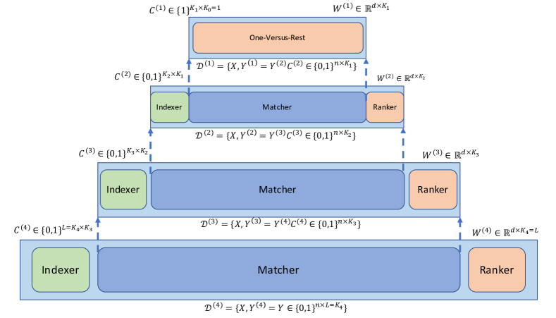
Figure 6: Illustration of XR-LINEAR.

3 XR-LINEAR

In this section, we present XR-LINEAR, a recursive realization of our PECOS framework proposed in Section 2. In particular, we exploit the property that the sub-problem handled by the matcher is also an XMR problem with a smaller output space of size $K$. Thus, we can further apply the three stage PECOS framework recursively.

Let $\mathopen{}\mathclose{{}\left\{{X,Y}}\right\}$ be the training matrices for the original XMR problem with $X\in\mathds{R}^{n\times d}$ and $Y\in\mathopen{}\mathclose{{}\left\{{0,1}}\right\}^{n\times L}$. Given an indexing matrix $C\in\mathopen{}\mathclose{{}\left\{{0,1}}\right\}^{L\times K}$, the ranker $h({\bm{x}},\ell)$ can be trained on $\mathopen{}\mathclose{{}\left\{{X,Y}}\right\}$ with negatives induced by $M=\text{binarize}\mathopen{}\mathclose{{}\left({YC}}\right)$ and/or $\hat{M}$, which is the predicted instance-to-cluster matrix by the matcher $g_{b}({\bm{x}})$ on the training feature matrix $X$. For the choice of ranker in XR-LINEAR, we consider the simple linear ranker proposed in Section 2.3.2. On the other hand, the training data to train the matcher $g({\bm{x}},k)$ is $\mathopen{}\mathclose{{}\left\{{X,M}}\right\}$. If $K$ is small enough, we can apply an OVR ranker or classifier to obtain $g({\bm{x}},k)$; otherwise, we can treat $\mathopen{}\mathclose{{}\left\{{X^{\prime}=X,Y^{\prime}=M}}\right\}$ as a smaller XMR problem and apply the PECOS 3-stage framework to learn the matcher. In particular, what we need is a smaller indexing matrix $C^{\prime}\in\mathopen{}\mathclose{{}\left\{{0,1}}\right\}^{L^{\prime}\times K^{\prime}}$, where $L^{\prime}=K$ is the size of the output space of the matcher.

In XR-LINEAR, we apply the above procedure recursively $D$ times. In particular, let

$$\mathopen{}\mathclose{{}\left\{{C^{t}\in\mathopen{}\mathclose{{}\left\{{0,1}}\right\}^{K_{t}\times K_{t-1}}:K_{0}=1,\ K_{D}=L,\ t=1,\ldots,D}}\right\}$$ (14)

be a series of indexing matrices used for each of the $D$ XMR sub-problems. When $t=D$, it corresponds to the original XMR problem on the given training dataset $\mathopen{}\mathclose{{}\left\{{X^{(D)}=X,Y^{(D)}=Y}}\right\}$. When $t=D-1$, we construct the XMR sub-problem induced by the matcher with the training dataset $\mathopen{}\mathclose{{}\left\{{X,\text{binarize}\mathopen{}\mathclose{{}\left({Y^{D}C^{D}}}\right)}}\right\}$. In general, the sub-problem for the matcher at the $t$-th layer forms a full XMR problem at the $(t-1)$-st layer. When $t=1$, the output space of the XMR sub-problem is small enough to be solved directly by an OVR ranker. In Algorithm 2, we present detailed steps on how to apply the three stage PECOS framework $D$ times in order to solve the original XMR problem. In Figure 6, we give an illustration by using a toy example with $D=4$. It is worth mentioning two special cases of XR-LINEAR. When $D=2$, XR-LINEAR is the same as the standard non-recursive three stage PECOS with an OVR linear matcher and a linear ranker. On the other hand, when $D=1$, XR-LINEAR is equivalent to vanilla linear OVR over all the labels.

Model Sparsification.

An XR-LINEAR model is composed of $D$ rankers $h^{(t)}({\bm{x}},\ell)$ parametrized by matrices $W^{t}\in\mathds{R}^{d\times K_{t}}$. As mentioned earlier in Section 1, naively storing the entire dense parameter matrices is not feasible. To overcome a prohibitive model size, we apply a common strategy [1, 37] to sparsify $W^{(t)}$. In particular, after the training process of each binary classification to obtain ${\bm{w}}^{(t)}_{\ell}$, we perform a (hard) thresholding operation to truncate parameters with magnitude smaller than a user given value $\epsilon\geq 0$ to zero. We can choose $\epsilon$ approximately so that the parameter matrices can be stored in the main memory. Model sparsification is essential to avoid running out of memory when both the number of input features $d$ and the number of labels $L$ are large. In addition to hard thresholding, we also explored the option to include $\mathopen{}\mathclose{{}\left\|{{\bm{w}}}}\right\|_{1}$ as the regularization and found that hard thresholding yields slightly better performance than L1 regularization.

Choice of Indexing Matrices.

XR-LINEAR described in Algorithm 2 is designed in a way to take any series of indexing matrices of the form specified in (14), which in fact can represent a family of hierarchical label clusterings. This means that if the original label set $\mathcal{Y}$ comes with a hierarchy which can be represented in a form as (14), this hierarchy can be directly used within XR-LINEAR. On the other hand, when such a label hierarchy is not available, we can still apply the semantic label indexing (clustering) approaches described in Section 2.1 to obtain a series of indexing matrices. In particular, as a byproduct of Algorithm 1 with $B$-ary partitions, when $K=B^{D-1}$ a series of indexing matrices are naturally formed as follows. $C^{(D)}=C\in\mathopen{}\mathclose{{}\left\{{0,1}}\right\}^{L\times K}$ and for $t<D$, $C^{(t)}\in\mathopen{}\mathclose{{}\left\{{0,1}}\right\}^{B^{t}\times B^{t-1}}$ with

$$\mathopen{}\mathclose{{}\left({C^{(t)}}}\right)_{lk} =\begin{cases}1&\text{ if }\mathopen{}\mathclose{{}\left\lceil{\frac{\ell}{B}}}\right\rceil=k,\\ 0&\text{ otherwise }\end{cases},\quad\forall\ 1\leq\ell\leq B^{t+1},\ 1\leq k\leq B^{t}.$$

This is essentially balanced hierarchical label clustering. With the choice of this hierarchical clustering, the size of the output spaces in the $D$ XMR problems are

$$K_{D}=L,K_{D-1}=B^{D-1},K_{D-2}=B^{D-2},\cdots,K_{1}=B^{1},$$

respectively.

Choice of Negative Sampling Schemes and Transform functions

XR-LINEAR in Algorithm 2 is flexible to adopt a different choice of negative sampling schemes and transform functions $\sigma^{(t)}(g,h)$ at each layer. In general, the best choices for all the layers are data dependent and can be obtained via a proper hyper-parameter tuning. After some explorations, we observe that the following choice gives reasonably good performance among all the datasets we tried: TFN with $\mathcal{L}_{3}$-hinge transformation (13) for the first $D-1$ layers, and TFN + MAN with the shortlisting transform function (12) for the $D$-th layer.

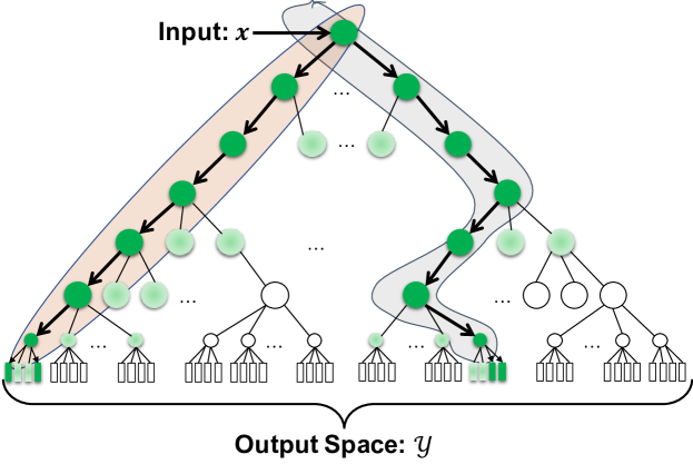
Figure 7: Illustration of the inference of XR-LINEAR using beam search with beam width $b=2$ to obtain $4$ relevant label predictions for the given input ${\bm{x}}$. The circular internal nodes denote label clusters at different levels of the label hierarchy, while the rectangular leaf nodes denote labels $\ell\in\mathcal{Y}$. We indicate in green color the label clusters which have been traversed during the beam search. Finally, the labels found relevant for the input ${\bm{x}}$ are the green rectangular leaf nodes.

3.1 Efficient Inference for XR-LINEAR

With the above choice of indexing matrices,Choice of Negative the inference for XR-LINEAR can be made very efficient with beam search. Beam search is a heuristic search algorithm to explore a directed graph (hierarchical label tree in our case) with a limited memory requirement. In particular, beam search is a variant of breadth-first search which only stores at most $b$ states at each level to further expand, where $b$ is also called beam size. In Figure 7, we give an illustration of how beam search works to perform inference in an XR-LINEAR model. Let $T_{h}$ be the time to compute $h^{(t)}({\bm{x}},\ell)$, the time complexity of inference via beam search with beam size $b$ becomes

$$\quad\sum_{t=1}^{D}\mathcal{O}\mathopen{}\mathclose{{}\left({\text{beam size}\times\max_{1\leq k\leq B^{t}}\ \mathopen{}\mathclose{{}\left|{\mathcal{Y}^{(t)}_{k}}}\right|\times T_{h}}}\right)$$

$$= \quad\sum_{t=1}^{D}\mathcal{O}\mathopen{}\mathclose{{}\left({b\times\frac{K_{t}}{K_{t-1}}\times T_{h}}}\right)\quad\quad\quad\quad\quad\quad\cdots\text{due to the balanced partitions}$$

$$= \quad\mathcal{O}\mathopen{}\mathclose{{}\left({D\times b\times\max\mathopen{}\mathclose{{}\left({B,\frac{L}{B^{D-1}}}}\right)\times T_{h}}}\right)\quad\cdots\text{due to the $B$-ary partitions}.$$

We can see that if $D$ and $B$ are chosen such that $L/B^{D-1}$ is a small constant (i.e., $D=\mathcal{O}(\log_{B}L)$) such as $100$, the overall time complexity of the inference for XR-LINEAR is

$$\mathcal{O}\mathopen{}\mathclose{{}\left({\log L\times b\times T_{h}}}\right),$$

which is logarithmic in the size of the original output space.

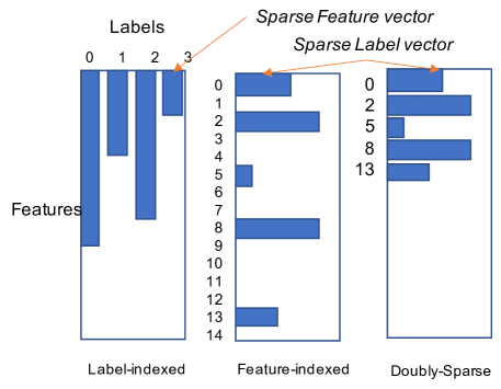
Figure 8: Sparse Data Structures for the weight matrix $W\in\mathds{R}^{d\times\mathopen{}\mathclose{{}\left|{\mathcal{Y}}}\right|}$ in a label cluster, $\mathcal{Y}$. The memory requirements from left to right are $\mathcal{O}(|\mathcal{Y}|+\text{nnz}(W))$, $\mathcal{O}(d+\text{nnz}(W))$ and $\mathcal{O}(\text{nnz}(W))$ respectively.

Efficient Ranking with Sparse Inputs.

Now we focus on how to efficiently rank the retrieved labels in real time when the XR-LINEAR model weights and the input vectors are sparse. For a given input ${\bm{x}}$, the score is defined as $h({\bm{x}},\ell)={\bm{w}}_{\ell}^{\top}{\bm{x}}$, where ${\bm{w}}_{\ell}$ is the weight vector for the $\ell$-th label. For sparse input data, such as tfidf features of text input, ${\bm{x}}$ is a sparse vector. By enforcing sparsity structure on the weight vectors during training, a key computational step becomes the multiplication of a sparse matrix and a sparse vector. However, many existing XMR linear classifiers, such as Parabel, are optimized for batch inference, i.e., the average time is optimized for a large batch of testing data. In many applications, we often need to do real-time inference, where the inputs arrive one at a time.

Here we propose a data structure called doubly-sparse representation for the weight vectors along with an algorithm to improve the speed of the real-time inference. Given a label cluster $\mathcal{Y}\subset[L]$, we aggregate the weight vectors in this cluster and form a weight matrix $W=[{\bm{w}}_{\ell}]_{\ell\in\mathcal{Y}}\in\mathds{R}^{d\times|\mathcal{Y}|}$, where $d$ is the number of features and $|\mathcal{Y}|$ is the number of labels in this cluster. In Figure 8, we illustrate several data structures to store the weight matrix. In the label-indexed representation, we store multiple (feature-index, value) pairs for each column of $W$. We call each column vector as a sparse feature vector. Note that Parabel [37] implements the label-indexed representation. In the feature-indexed representation, we store multiple (label-index, value) pairs for each row of $W$. We call each row vector as a sparse label vector. Each row of the weight matrix is recorded even if it is empty. In the doubly sparse representation, we store only the non-empty sparse label vectors and the corresponding row indices.

Note that when the label cluster only contains a small set of labels and the feature dimension is very large, the weight matrix will be very sparse, i.e., $\text{nnz}(W)<d$, and the feature-indexed representation will consume a lot of memory to store an empty vector for each feature. Therefore, to achieve efficient real-time inference for a XR-LINEAR model, we propose to use the doubly sparse representation, which is based on feature-indexed representation but only stores non-empty label vectors. There are two data structures we can utilize to quickly find a given row index: 1) store the row indices of the non-empty label vectors in a sorted array and use binary search, 2) use a hash table to map the row indices to label vectors. For simplicity, we focus on using a hash table in this paper.

Given an input data, ${\bm{x}}$, and a weight matrix $W$, our goal is to calculate the scores for the labels, i.e., $W^{\top}{\bm{x}}$. In the feature-indexed representation, we can find the sparse label vector for the index of any non-zero feature of the input ${\bm{x}}$ in a constant time, therefore, the computational complexity is $\mathcal{O}(\text{nnz}({\bm{x}})+\text{nnz}(W))$. However, the memory requirement will be $\mathcal{O}(d+\text{nnz}(W))$ for each weight matrix. For some datasets, such as Wiki-500K ($d\approx 500,000$ and $K\approx 5,000$), the total memory required can be huge. In the label-indexed representation, $W^{\top}{\bm{x}}$ consists of $\mathopen{}\mathclose{{}\left|{\mathcal{Y}}}\right|$ inner products between two sparse vectors. As implemented in the Parabel code [43], for every inner-product, it first transforms a sparse weight vector to a dense vector and then uses (sparse-matrix, dense-vector) multiplication to calculate the inner product between the weight vector and the input vector. Therefore, the computational complexity is $\mathcal{O}(\mathopen{}\mathclose{{}\left|{\mathcal{Y}}}\right|\times\text{nnz}({\bm{x}})+\text{nnz}(W))$. To reduce both the computational complexity and memory requirement, we use a doubly-sparse weight matrix. We still use (label-index, value) pairs to store each non-empty row in the weight matrix. We use a hash table to map the feature indices to the non-empty rows. Although the hashing step is slightly slower than direct memory access as in feature-indexed representation, it still has an amortized constant time. Given a sparse input, we can get the corresponding rows from the non-zero feature indices in constant time, therefore, the computational complexity for calculating $W^{\top}{\bm{x}}$ is only $\mathcal{O}(\text{nnz}({\bm{x}})+\text{nnz}(W))$ while using $\mathcal{O}(\text{nnz}(W))$ memory. We list the time and memory complexity of the overall inference in Table 1.

Table 1: Time and memory complexity of the inference. Here $b$: beam size. $\text{nnz}(\hat{w})$: average number of non-zeros of the weight vectors. $D$: the depth of the tree ($D=\mathcal{O}(\log L)$).

Data Structure	Computational Complexity	Memory Usage
Label-indexed	$b\times(\text{nnz}({\bm{x}})+\text{nnz}(\hat{w}))\times(D+L/B^{D-1})$	$\text{nnz}(\hat{w})\times L$
Feature-indexed	$b\times\text{nnz}({\bm{x}})\times D+b\times\text{nnz}(\hat{w})\times(D+L/B^{D-1})$	$\text{nnz}(\hat{w})\times L+d\times B^{D}$
Doubly-sparse	$b\times\text{nnz}({\bm{x}})\times D+b\times\text{nnz}(\hat{w})\times(D+L/B^{D-1})$	$\text{nnz}(\hat{w})\times L$

In summary, feature-indexed representation is the fastest but takes too much memory when $d$ is very large. The doubly sparse representation is slightly slower than the feature-indexed representation due to the hashing step but is much more memory-efficient. Therefore, we recommend doubly sparse representation and use it for the experimental results in Table 5 of Sec. 6.3. In [13], we apply doubly sparse representation (called Masked Sparse Chunk Multiplication in [13]) to different algorithms for sparse extreme multi-label ranking trees and achieve faster inference than methods in Parabel [37] and NAPKINXC [19].

4 Deep Learned Matchers for Text Inputs

In this section, we present deep learned matchers for XMR problems with text inputs. Note that unlike XR-LINEAR which can handle general inputs where the features are in vector form, the techniques discussed in this section only apply to XMR problems with text inputs. Let ${\bm{t}}_{i}$ denote the text sequence associated with the $i$-th input. Let ${\bm{x}}=\mathbf{\bm{\phi}}({\bm{t}}\mid\Theta)$ denote a vectorizer function which converts the input text sequence ${\bm{t}}$ to a $d$-dimensional feature vector ${\bm{x}}$, where $\Theta$ is the parameter controlling the vectorizer. For example, a term frequency-inverse document frequency (tfidf) vectorizer, $\mathbf{\bm{\phi}}_{\text{tfidf}}({\bm{t}}\mid\Theta_{\text{tfidf}})$ is parameterized by a vocabulary $\mathcal{V}$ and the inverse document frequency of each term $\mathopen{}\mathclose{{}\left\{{\text{idf}(v):\forall v\in\mathcal{V}}}\right\}$. For an XMR problem with text inputs, PECOS with a tfidf vectorizer works reasonably well in our experience. However, the parameters $\Theta$ for traditional text vectorizers such as tfidf are obtained using only the text of the training set and are independent from the supervision $Y$ provided in the training set.

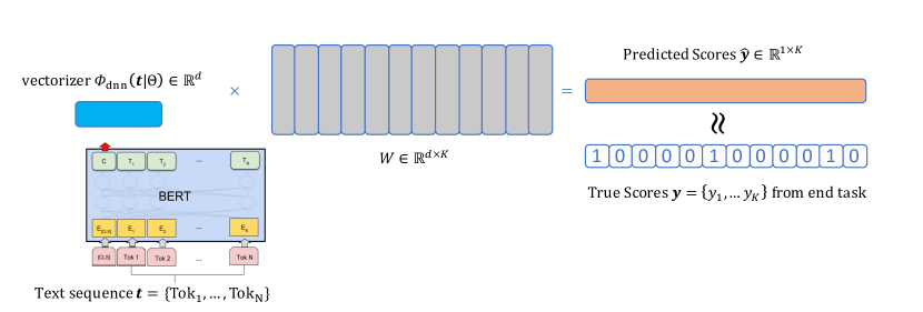
Figure 9: Illustration of fine-tuning a pre-trained Transformer model such as BERT [9] to a given end task.

Recently, deep pre-trained Transformers, e.g., BERT [9] along with its many successors such as XLNet [50] and RoBERTa [29], have led to state-of-the-art performance on many NLP tasks, such as question answering, part-of-speech tagging, and sentence classification with very few labels. Deep pretrained Transformer models provide a trainable text vectorizer that can be rapidly fine-tuned on many downstream NLP problems by adding a task-specific lightweight linear layer on top of the Transformer models as illustrated in Figure 9. In particular, the text vectorizer from a given Transformer model can be represented as $\mathbf{\bm{\phi}}_{\text{dnn}}({\bm{t}}\mid\Theta)$, where $\Theta$ denotes the weights for the deep neural network architecture. Although the pretrained $\Theta$ is usually obtained by learning a general language model on a large text corpus, it can be fined-tuned on various downstream NLP tasks, such as those in the GLUE benchmark [45].

We consider incorporating such a trainable deep text vectorizer so we have a deep learned matcher:

$$g_{\text{dnn}}({\bm{t}},k)={\bm{w}}_{k}^{\top}\mathbf{\bm{\phi}}_{\text{dnn}}({\bm{t}}\mid\Theta).$$

Note that the first argument of $g$ is the text sequence ${\bm{t}}$ instead of the feature vector ${\bm{x}}$. Recall that the sub-problem to learn our matcher is also an XMR problem, where the training data is $\mathopen{}\mathclose{{}\left\{{X,M}}\right\}$. Note that when we have millions of labels, using trainable deep vectorizers on the original problem $\mathopen{}\mathclose{{}\left\{{X,Y}}\right\}$ would be prohibitive. If an OVR approach is used to learn the matcher, we can solve the following fine-tuning problem to obtain the parameters for our deep learned matcher:

$$\min_{\mathopen{}\mathclose{{}\left\{{{\bm{w}}_{k}}}\right\},\Theta}\quad\sum_{i=1}^{n}\sum_{k=1}^{K}\mathcal{L}\mathopen{}\mathclose{{}\left({M_{ik},{\bm{w}}_{k}^{\top}\mathbf{\bm{\phi}}_{\text{dnn}}({\bm{t}}_{i}\mid\Theta)}}\right),$$ (15)

where $\mathcal{L}(\cdot,\cdot)$ is a loss function and $M=\text{binarize}(YC)$ is the instance-to-cluster matrix. In particular, we use $\mathcal{L}_{\text{squared-hinge}}$ loss in our experiments as it has shown better performance in existing XMR work [52, 37]. Due to the use of a deep text vectorizer $\mathbf{\bm{\phi}}_{\text{dnn}}({\bm{t}}\mid\Theta)$ and having $\Theta$ as a trainable parameter in (15), we follow the providers of the pre-trained models and use a variant of the Adam algorithm [23] to solve (15). Below we summarize our learnings in this exploration.

Choice of Deep Text Vectorizers.

We consider three state-of-the-art pre-trained Transformer-large-cased models (i.e., 24 layers with case-sensitive vocabulary) as our deep text vectorizers, namely BERT [9], XLNet [50], and RoBERTa [29]. In terms of training speed, BERT and RoBERTa are similar while XLNet is nearly $1.8$ times slower. In terms of performance on XMR tasks, we found RoBERTa and XLNet to be slightly better than BERT, but the gap is not significant.

Training Efficiency.

The time and space complexity of the Transformer scales quadratically with the input sequence length [44], i.e., $\mathcal{O}(T^{2})$, where $T=\text{len}({\bm{t}})$ is the number of tokenized sub-words in the instance ${\bm{t}}$. Using smaller $T$ reduces not only the GPU memory usage that supports using larger batch size, but also increases the training speed. For example, BERT [9] first pre-trains on inputs of sequence length $128$ for $90\%$ of the optimization, and the remaining $10\%$ of optimization steps on inputs of sequence length $512$. Interestingly, we observe that the model fine-tuned with sequence length $128$ v.s. sequence length $512$ does not differ significantly in downstream XMR performance. Thus, we fix the input sequence length to be $T=128$ for model fine-tuning, which significantly speeds up the training time. It would be interesting to see if we can bootstrap training the Transformer models from shorter sequence length and ramp up to larger sequence length (e.g., 32, 64, 128, 256), but we leave that as future work.

Recursive Realization with Shared Encoder.

Intuitively, the recursive realization with deep learned matchers would involve multiple deep learning text encoders. However, in practice, sharing the text encoder across all the hierarchical layers would be a better choice. On one hand, the inference time is dominated by the evaluation of text embeddings and having multiple text encoders would greatly increase the inference latency. On the other hand, having a shared encoder means that the same neural network can be trained on multi-resolution label signals, which is proven to improve both training efficiency and model performance. More details can be found in Zhang et al. [54, Section 4].

Further Utilization of Learned Deep Text Vectorizer.

As a byproduct of our deep learned matcher, we have a powerful deep text vectorizer $\mathbf{\bm{\phi}}_{\text{dnn}}\mathopen{}\mathclose{{}\left({{\bm{t}}\mid\Theta_{\text{fnt}}}}\right)$, where $\Theta_{\text{fnt}}$ denotes the fine-tuned parameters after solving (15). This vectorizer can be further utilized to further improve the overall XMR performance. First, we can concatenate it with a simple tfidf vectorizer to form the feature vector for our ranker. In particular, we can have

$${\bm{x}}_{i}^{\top}=\mathopen{}\mathclose{{}\left[{\mathbf{\bm{\phi}}_{\text{tfidf}}^{\top}\mathopen{}\mathclose{{}\left({{\bm{t}}_{i}\mid\Theta_{\text{tfidf}}}}\right),\ \mathbf{\bm{\phi}}_{\text{dnn}}^{\top}\mathopen{}\mathclose{{}\left({{\bm{t}}_{i}\mid\Theta_{\text{fnt}}}}\right)}}\right]$$

as the feature vector for the $i$-th instance to train the simple linear ranker. We observe that such concatenation leads to the best overall performance compared to the use of either tfidf or Deep Text Vectorizer individually. Second, as mentioned earlier in Section 2.4, we can use this deep learned text vectorizer to form a new set of feature vectors and learn a new model based on it, which we can then ensemble with the model based on tfidf vectorizer.

5 Related Work

5.1 Sparse Linear Models with Partitioning Techniques

Conventional XMR algorithms consider fixed input representations such as sparse tfidf features and leverage different partitioning techniques or surrogate loss functions on the large label space to reduce complexity. For example, sparse linear one-versus-reset (OVR) methods such as DiSMEC [1], ProXML [2], PPDSparse [51, 52] explore parallelism to speed up the algorithm and reduce the model size by truncating model weights to encourage sparsity.

The efficiency and scalability of OVR models can be further improved by incorporating different partitioning techniques on the label spaces. For instance, Parabel [37] partitions the labels through a balanced 2-means label tree using label features constructed from the instances. Other approaches attempt to improve on Parabel, for instance, eXtremeText [49], Bonsai [22], and NAPKINXC [19] relax two main constraints in Parabel by: 1) allowing multi-way instead of binary partitions of the label set at each intermediate node, and 2) removing strict balancing constraints on the partitions. On the other hand, SLICE [18] and AnnexML [42] partition the label spaces via graph-based approximate nearest neighbor (ANN) indices. For a given instance, relevant labels can be found quickly from nearest neighbors of the instance via the ANN graph.

Comparing PECOS with Parabel.

Concerning the three phase framework for PECOS, we can interpret Parabel [37] as a special case of XR-LINEAR with the following choices: PIFA label representation + Algorithm 1 (with $B=2$) + TFN sampling scheme. There are three main differences between XR-LINEAR and Parabel. First, XR-LINEAR generalizes Parabel with multi-way partitioning of the hierarchical label tree. Second, XR-LINEAR incorporates various hard negative sampling schemes (e.g., MAN, TFN+MAN). Finally, even if the model parameters are the same for XR-LINEAR and Parabel, XR-LINEAR achieves significantly lower real-time inference latency because of the doubly-sparse data structure described in Sections 3.1 and  6.3.

5.2 Neural Embedding-based Models

Neural-based XMR models employ various network architectures to learn semantic embeddings of the input text. XML-CNN [27] employs one-dimensional CNN on the input sequence and train the model with binary cross entropy loss without sampling, which is not scalable to large label spaces. Shallow embedding-based methods aggregate word embeddings of a text input followed by shallow MLP layers to obtain input embeddings, which has smaller encoding latency for real-time inference. Specifically, DeepXML [8] and its variant (i.e., DECAF [32], GalaXC [39], ECLARE [33]) pre-train MLP encoders on XMR sub-problems induced by label clusters. They freeze the pre-trained word embedding and learn another MLP layer with hard negative labels from HNSW [30]. Notably, shallow embedding-based methods only show competitive performance on short-text XMR problems where the number of input tokens is small.

To better handle longer text sequence, AttentionXML [53] uses BiLSTMs and label-aware attention as the scoring function. For better scalability to large output spaces, training of AttentionXML involves various negative sampling strategies to avoid back-propagating the entire label embedding layer. More recently, LightXML [20] adopts the transformer models as text encoder, and performs label shortlist and re-ranking with the same transformer encoder. By capturing rich semantic information from input text, LightXML establishes competitive results on public XMR benchmarks.

Comparing PECOS with AttentionXML.

PECOS induces two neural-based realizations using Transformer encoders, which are X-TRANSFORMER [7] and XR-TRANSFORMER [54]. There are three main differences between XR-TRANSFORMER and AttentionXML. First, XR-TRANSFORMER captures better semantic embeddings for long text sequence using Transformers. Second, XR-TRANSFORMER can easily leverage any pre-trained Transformer models from the literature. Finally, XR-TRANSFORMER is optimized with cost-sensitive loss induced by recursive course-to-fine signals.

6 Experimental Results

In this section, we compare various realization of PECOS with recent XMR models on six real-world extreme multi-label text classification datasets: Eurlex-4K, Wiki10-31K, AmazonCat-13K, Wiki-500K, Amazon-670K and Amazon-3M. Details of these datasets and its statistics are presented in Table 2. We use the same raw text input, sparse feature representations, and training/test data split as in  You et al. [53], Chang et al. [7], Zhang et al. [54], Jiang et al. [20] to have a fair and reproducible comparison.

Table 2: Data Statistics. $n_{\text{trn}},n_{\text{tst}}$ refer to the number of instances in the training and test sets, respectively. $\mathopen{}\mathclose{{}\left|{\mathcal{D}_{\text{trn}}}}\right|,\mathopen{}\mathclose{{}\left|{\mathcal{D}_{\text{tst}}}}\right|$ refer to the number of word tokens in the training and test corpus, respectively. $d$ is the dimension of tfidf feature vector. $L$ is the number of labels, $\bar{L}$ the average number of labels per instance, $\bar{n}$ the average number of instances per label. These six publicly available benchmark datasets are downloaded from https://github.com/yourh/AttentionXML which are the same as AttentionXML [53] for fair comparison.

Dataset	$n_{\text{trn}}$	$n_{\text{tst}}$	$\mathopen{}\mathclose{{}\left|{\mathcal{D}_{\text{trn}}}}\right|$	$\mathopen{}\mathclose{{}\left|{\mathcal{D}_{\text{tst}}}}\right|$	$d$	$L$	$\bar{L}$	$\bar{n}$
Eurlex-4K	15,449	3,865	19,166,707	4,741,799	186,104	3,956	5.30	20.79
Wiki10-31K	14,146	6,616	29,603,208	13,513,133	101,938	30,938	18.64	8.52
AmazonCat-13K	1,186,239	306,782	250,940,894	64,755,034	203,882	13,330	5.04	448.57
Wiki-500K	1,779,881	769,421	1,463,197,965	632,463,513	2,381,304	501,070	4.75	16.86
Amazon-670K	490,449	153,025	119,981,978	36,509,660	135,909	670,091	5.45	3.99
Amazon-3M	1,717,899	742,507	174,559,559	75,506,184	337,067	2,812,281	36.04	22.02

Table 3: Comparison of XR-LINEAR, X-TRANSFORMER and XR-TRANSFORMER with recent XMR methods on six publicly available datasets. Results of non-PECOS models are taken from You et al. [53, Table 3] and Jiang et al. [20, Table 2]. The results show that XR-TRANSFORMER achieves state-of-the-art precision numbers.

Methods	Prec@1	Prec@3	Prec@5	Methods	Prec@1	Prec@3	Prec@5
Eurlex-4K				Wiki10-31K
AnnexML	79.66	64.94	53.52	AnnexML	86.46	74.28	64.20
DiSMEC	83.21	70.39	58.73	DiSMEC	84.13	74.72	65.94
PfastreXML	73.14	60.16	50.54	PfastreXML	83.57	68.61	59.10
Parabel	82.12	68.91	57.89	Parabel	84.19	72.46	63.37
eXtremeText	79.17	66.80	56.09	eXtremeText	83.66	73.28	64.51
Bonsai	82.30	69.55	58.35	Bonsai	84.52	73.76	64.69
fastText	71.59	60.51	51.07	fastText	82.26	65.93	55.25
XML-CNN	75.32	60.14	49.21	XML-CNN	81.41	66.23	56.11
AttentionXML	87.12	73.99	61.92	AttentionXML	87.47	78.48	69.37
LightXML	87.63	75.89	63.36	LightXML	89.45	78.96	69.85
XR-LINEAR	82.07	69.61	58.23	XR-LINEAR	84.55	73.02	64.24
X-TRANSFORMER	87.61	75.39	63.05	X-TRANSFORMER	88.26	78.51	69.68
XR-TRANSFORMER	88.41	75.97	63.18	XR-TRANSFORMER	88.69	80.17	70.91
AmazonCat-13K				Wiki-500K
AnnexML	93.54	78.36	63.30	AnnexML	64.22	43.15	32.79
DiSMEC	93.81	79.08	64.06	DiSMEC	70.21	50.57	39.68
PfastreXML	91.75	77.97	63.68	PfastreXML	56.25	37.32	28.16
Parabel	93.02	79.14	64.51	Parabel	68.70	49.57	38.64
eXtremeText	92.50	78.12	63.51	eXtremeText	65.17	46.32	36.15
NAPKINXC	93.04	78.44	63.70	NAPKINXC	66.77	47.63	36.94
Bonsai	92.98	79.13	64.46	Bonsai	69.26	49.80	38.83
fastText	90.55	77.36	62.92	fastText	31.59	18.47	13.47
XML-CNN	93.26	77.06	61.40	XML-CNN	-	-	-
AttentionXML	95.92	82.41	67.31	AttentionXML	76.95	58.42	46.14
LightXML	96.77	84.02	68.70	LightXML	77.78	58.85	45.57
XR-LINEAR	92.97	78.94	64.30	XR-LINEAR	68.12	49.07	38.39
X-TRANSFORMER	96.48	83.41	68.19	X-TRANSFORMER	77.09	57.51	45.28
XR-TRANSFORMER	96.79	83.66	68.04	XR-TRANSFORMER	79.40	59.02	46.25
Amazon-670K				Amazon-3M
AnnexML	42.09	36.61	32.75	AnnexML	49.30	45.55	43.11
DiSMEC	44.78	39.72	36.17	DiSMEC	47.34	44.96	42.80
PfastreXML	36.84	34.23	32.09	PfastreXML	43.83	41.81	40.09
Parabel	44.91	39.77	35.98	Parabel	47.42	44.66	42.55
eXtremeText	42.54	37.93	34.63	eXtremeText	42.20	39.28	37.24
NAPKINXC	43.54	38.71	35.15	NAPKINXC	46.23	43.48	41.41
Bonsai	45.58	40.39	36.60	Bonsai	48.45	45.65	43.49
fastText	24.35	21.26	19.14	fastText	22.51	19.05	16.99
XML-CNN	33.41	30.00	27.42	XML-CNN	-	-	-
AttentionXML	47.58	42.61	38.92	AttentionXML	50.86	48.04	45.83
LightXML	49.10	43.83	39.85	LightXML	-	-	-
XR-LINEAR	45.36	40.35	36.71	XR-LINEAR	47.96	45.09	42.96
X-TRANSFORMER	48.07	42.96	39.12	X-TRANSFORMER	51.20	47.81	45.07
XR-TRANSFORMER	50.11	44.56	40.64	XR-TRANSFORMER	54.20	50.81	48.26

In Section 6.1, we focus on the performance of various models and demonstrate that XR-TRANSFORMER, a realization of PECOS framework with a recursive Transformer matcher, achieves state-of-the-art prediction performance. In Section 6.2, we show that XR-LINEAR (Section 3), a linear counterpart of XR-TRANSFORMER, achieves satisfactory prediction performance while requiring substantially less training time. In Section 6.3, we demonstrate that the efficiency of the inference procedure for XR-LINEAR, which allows it to serve real-time requests. Finally, in Section 6.4, we present the ablation study of XR-LINEAR to examine the effectiveness of semantic label clustering and model ensembling.

6.1 Performance Comparison

To compare the predictive performance of various models, we use the widely used precision and recall metrics for the XMR task [36, 4, 17, 37, 38]. In particular, for an input ${\bm{x}}$ and the corresponding ground truth ${\bm{y}}\in\mathcal{Y}$, the Prec@$p$ ($p=1,3,5$) and Recall@$p$ ($p=1,3,5$) for the top-$b$ predictions $f_{b}({\bm{x}})$ are defined as follows:

$$\text{Prec}@b=\frac{1}{b}\sum_{\ell\in f_{b}({\bm{x}})}y_{\ell},\quad\text{Recall}@b=\frac{1}{\text{nnz}({\bm{y}})}\sum_{\ell\in f_{b}({\bm{x}})}y_{\ell}.$$

We consider three PECOS instantiations:

• XR-LINEAR: We use PIFA as label embeddings to construct the hierarchical label tree (HLT) with branching factor $B=32$ in Algorithm 1. We use TFN as the negative sampling in Algorithm 2. Similar to Parabel [37], we use beam size $b=10$ and an ensemble of three HLTs for the prediction stage.

• X-TRANSFORMER: PECOS with non-recursive Transformer matchers. Predictions are an ensemble of 9 X-TRANSFORMER models with three encoders and three HLTs. Detailed specifications and hyperparameters can be found in Chang et al. [7, Section 4.2].

• XR-TRANSFORMER: PECOS with recursive Transformer matchers. Predictions are an ensemble of 3 XR-TRANSFORMER models with three encoders. Detailed specifications and hyperparameters can be found in Zhang et al. [54, Section 5].

We then include the following XMR models in our comparisons.

• Embedding-based Approaches: AnnexML [42]

• OVR-based Approaches: DiSMEC [1]

• Tree-based Approaches: PfastreXML [17], Parabel [37], eXtremeText [49], Bonsai [22], and NAPKINXC [19].

• Deep learning-based Approaches: fastText [21], XML-CNN [27], AttentionXML [53] and LightXML [20].

Note that in terms of our three phase framework for PECOS, Parabel [37] may be interpreted as a special case of XR-LINEAR with the following special choices: PIFA label representation + Algorithm 1 (with $B=2$) + TFN negative sampling scheme. In other words, XR-LINEAR with $B=32$ in Table 3 has a smaller depth of hierarchical label tree, which enjoys faster inference time in practice.

Table 3 shows that our proposed XR-TRANSFORMER method outperforms other competitive deep learning based XMR methods (e.g., AttentionXML and LightXML) on most metrics, especially on datasets with large output spaces such as Amazon-670K and Amazon-3M. This verifies the effectiveness of recursive learning of transformer encoders on large output space problems. While X-TRANSFORMER and XR-TRANSFORMER results in better predictive performance compared to its linear counterpart XR-LINEAR, they also requires considerably longer training time, as we will see in the Section 6.2.

Table 4: Training time (in seconds) versus predictive performance of various PECOS realizations.

0.90 Eurlex-4K ($\mathopen{}\mathclose{{}\left|{\mathcal{Y}}}\right|=3,956,\ n_{\text{trn}}=15,449,\ n_{\text{tst}}=3,865$) Model Training Prec@1 Prec@3 Prec@5 Recall@1 Recall@3 Recall@5 Time (s) XR-TRANSFORMER 88.41 75.97 63.18 17.93 45.26 61.49 2,880.0 X-TRANSFORMER 87.61 75.39 63.05 17.78 44.92 61.35 26,766.0 XR-LINEAR     TFN 82.07 69.61 58.23 16.59 41.36 56.60 7.4     TFN+MAN 83.08 69.87 58.18 16.81 41.55 56.52 20.2 Wiki10-31K ($\mathopen{}\mathclose{{}\left|{\mathcal{Y}}}\right|=30,938,\ n_{\text{trn}}=14,146,\ n_{\text{tst}}=6,616$) Model Training Prec@1 Prec@3 Prec@5 Recall@1 Recall@3 Recall@5 Time (s) XR-TRANSFORMER 88.69 80.17 70.91 5.30 14.17 20.44 5.400.0 X-TRANSFORMER 88.26 78.51 69.68 5.28 13.76 19.79 51,815.0 XR-LINEAR     TFN 84.55 73.02 64.24 4.99 12.72 18.40 36.0     TFN+MAN 84.70 73.86 64.76 5.02 12.92 18.57 70.9 AmazonCat-13K ($\mathopen{}\mathclose{{}\left|{\mathcal{Y}}}\right|=13,330,\ n_{\text{trn}}=1,186,239,\ n_{\text{tst}}=306,782$) Model Training Prec@1 Prec@3 Prec@5 Recall@1 Recall@3 Recall@5 Time (s) XR-TRANSFORMER 96.79 83.66 68.19 27.69 63.31 79.37 47,520.0 X-TRANSFORMER 96.48 83.41 68.19 27.52 63.11 79.30 531,308.0 XR-LINEAR     TFN 93.06 78.95 64.28 26.33 59.78 75.20 220.2     TFN+MAN 93.06 78.95 64.20 26.30 59.77 75.17 1,074.3 Wiki-500K ($\mathopen{}\mathclose{{}\left|{\mathcal{Y}}}\right|=501,070,\ n_{\text{trn}}=1,779,881,\ n_{\text{tst}}=769,421$) Model Training Prec@1 Prec@3 Prec@5 Recall@1 Recall@3 Recall@5 Time (s) XR-TRANSFORMER 79.40 59.02 46.25 26.59 49.61 59.53 136,800.0 X-TRANSFORMER 77.09 57.51 45.28 25.51 48.03 58.05 2,005,550.0 XR-LINEAR     TFN 68.12 49.07 38.39 22.18 40.72 49.21 2,796.6     TFN+MAN 68.77 48.24 37.07 22.57 40.33 47.87 19,356.2 Amazon-670K ($\mathopen{}\mathclose{{}\left|{\mathcal{Y}}}\right|=670,091,\ n_{\text{trn}}=490,449,\ n_{\text{tst}}=153,025$) Model Training Prec@1 Prec@3 Prec@5 Recall@1 Recall@3 Recall@5 Time (s) XR-TRANSFORMER 50.11 44.56 40.64 10.52 26.02 38.29 37,800.0 X-TRANSFORMER 48.07 42.96 39.12 9.94 24.90 36.71 1,853,263.0 XR-LINEAR     TFN 45.36 40.35 36.71 9.44 23.43 34.45 147.2     TFN+MAN 45.81 40.64 36.82 9.63 23.67 34.61 928.4 Amazon-3M ($\mathopen{}\mathclose{{}\left|{\mathcal{Y}}}\right|=2,812,281,\ n_{\text{trn}}=1,717,899,\ n_{\text{tst}}=742,507$) Model Training Prec@1 Prec@3 Prec@5 Recall@1 Recall@3 Recall@5 Time (s) XR-TRANSFORMER 54.20 50.81 48.26 3.93 9.59 13.99 105,480.0 X-TRANSFORMER 51.20 47.81 45.07 3.28 8.03 11.65 1,951,324.0 XR-LINEAR     TFN 47.96 45.09 42.96 3.04 7.54 11.12 1,453.5     TFN+MAN 48.64 45.90 43.76 3.28 8.05 11.81 4,971.6

6.2 Training Time versus Predictive Performance

In this section, we analyze various PECOS realizations based on their training time and predictive performance. All the experiments of XR-LINEAR are run on a r5.24xlarge AWS instance, which contains 96 Intel Xeon Platinum 8000 CPUs and 768 GB RAM. All the experiments of X-TRANSFORMER and XR-TRANSFORMER, are obtained on a p3.16xlarge AWS instance, which contains 8 Nvidia V100 GPUs.

Experimental results are shown in Table 4, which include two variants of XR-LINEAR with different negative mining (i.e., TFN, TFN+MAN). We can clearly see that XR-LINEAR is the most efficient approach in terms of training time, followed by XR-TRANSFORMER and then X-TRANSFORMER. In particular, XR-LINEAR with TFN negative sampling is often 2x to 5x faster than XR-LINEAR with TFN+MAN sampling, because the latter requires model inference on the large training set to generate hard negative based on the model parameters. Nevertheless, XR-LINEAR with TFN+MAN may lead to better predictive performance on larger output space datasets such as Amazon-3M.

Compared to XR-LINEAR, on the other hand, X-TRANSFORMER and XR-TRANSFORMER yield state-of-the-art precision and recall results at the cost of larger training time, where XR-TRANSFORMER is often 10x faster than X-TRANSFORMER. This verifies the effectiveness of recursive training for Transformer matchers on the large output space datasets. It is noteworthy that PECOS is flexible to have realizations like XR-TRANSFORMER which yields the best prediction performance and realizations like XR-LINEAR which strikes a good balance between prediction performance and training cost. Note that even though relatively cheaper compared with X-TRANSFORMER, the XR-TRANSFORMER method still requires faster and more expensive GPU hardware. This flexibility allows practitioners to choose the most appropriate PECOS model for their applications.

6.3 Real-Time Inference

Next, we compare the real-time inference latency of various PECOS realization with competitive XMR methods. Specifically, in real-time mode, we consider the test instances are fed one-by-one to the model. Table 5 compares the inference latency (milliseconds per input instance) among Parabel, XR-LINEAR, NAPKINXC, X-TRANSFORMER and XR-TRANSFORMER in real time mode. Real-time experiments for Parabel, NAPKINXC and XR-LINEAR are conducted on a AWS instance r5.4xlarge using single thread while X-TRANSFORMER and XR-TRANSFORMER are evaluated on a Tesla V100 GPU. In our experiments, we randomly sampled 10,000 test inputs/instances for reporting the numbers in Table 5.

We implemented our version of Parabel and NAPKINXC for fair comparison in the real-time inference case. The original Parabel code is designed for batch input mode, so it is slow in real-time mode. Parabel, XR-LINEAR, NAPKINXC all use the same model parameters and same number of branch splits, $B=32$. XR-LINEAR and NAPKINXC use hash method to look up the non-empty rows. Beam size and topk are both set to 10 for all experiments in Table 5.

As we can see, XR-LINEAR is much faster than NAPKINXC and Parabel across all datasets. X-TRANSFORMER and XR-TRANSFORMER are deep learning models which achieve better precision and recall but require much larger inference time due to expensive transformer encoders.

1

Table 5: Online Inference Latency (milliseconds per input) for Parabel, NAPKINXC, XR-LINEAR, XR-TRANSFORMER and X-TRANSFORMER. X-TRANSFORMER and XR-TRANSFORMER are evaluated on a Nvidia Tesla V100 GPU while other models are evaluated on an AWS instance r5.4xlarge using a single thread.

	Eurlex-4K	Wiki10-31K	AmazonCat-13K	Wiki-500K	Amazon-670K	Amazon-3M
Parabel	1.20	5.77	17.00	175.00	10.70	44.60
NAPKINXC	1.63	7.10	1.93	12.60	2.80	3.59
XR-LINEAR	0.20	1.06	0.33	2.26	0.48	0.61
X-TRANSFORMER	433.87	433.20	428.58	433.33	432.24	451.97
XR-TRANSFORMER	66.90	117.30	78.30	101.70	92.70	105.60

6.4 Ablation Study of XR-LINEAR

In Table 6, we compare different configurations of hierarchical label tree (HLT) as the ablation study of XR-LINEAR. The experiment results are conducted on an r5.24xlarge AWS instance, which contains 96 Intel Xeon Platinum 8000 CPUs and 768 GB RAM. Note that we use the multi-threading batch-mode for model predictions and report the total prediction time in seconds.

First, we investigate different tree depths of HLT by vary branching splits $B=\{2,8,32\}$. From Table 6, we observed that $B=32$ (shallower HLTs) usually results in better predictive performance compared to $B=2$ (deeper HLTs). Furthermore, the prediction time of shallower HLTs are also faster than the prediction time of deeper HLTs, which justifies the default choice of $B=32$ for experiments of all previous sections. We also explore a randomly clustered HLT on Eurlex-4K, where the Prec@k drops to 79.3, 67.1, and 55.9, for $k=1,3,5$, respectively. Given this significant drop, we omit the results of random clusters in Table 6.

Finally, we compare the performance versus training time of a single HLT ($T=1$) versus an ensemble of three HLTs ($T=3$). From Table 6, XR-LINEAR with $T=3$ has better precision and recall compared to XR-LINEAR with $T=1$. However, it also comes with the price of larger training and prediction time.

Table 6: Ablation study of XR-LINEAR with respective to different configurations of the hierarchical label tree (HLT). $T$ is the number of HLT, where $T=1$ refers to XR-LINEAR with a single HLT while $T=3$ refers to XR-LINEAR with an ensemble of three HLTs. $B$ and $D$ are the branching splits and depth of HLT, respectively. Training time and prediction time (in seconds) are measured on an r5.24xlarge AWS instance, which contains 96 Intel Xeon Platinum 8000 CPUs and 768 GB RAM. Note that we use TFN sampling to train the model and consider beam size $b=10$ for the model prediction using multi-threading batch-mode.

1.0 Eurlex-4K ($\mathopen{}\mathclose{{}\left|{\mathcal{Y}}}\right|=3,956,\ n_{\text{trn}}=15,449,\ n_{\text{tst}}=3,865$) $T$ $B$ $D$ Prec@1 Prec@3 Prec@5 Recall@1 Recall@3 Recall@5 Train Time Predict Time 3 2 7 81.47 69.13 57.87 16.51 41.10 56.28 8.70 0.28 3 8 3 81.79 69.30 58.04 16.54 41.16 56.46 7.40 0.32 3 32 3 82.07 69.61 58.23 16.59 41.36 56.60 7.47 0.28 1 32 3 82.48 68.83 57.61 16.65 40.85 55.98 2.49 0.09 Wiki10-31K ($\mathopen{}\mathclose{{}\left|{\mathcal{Y}}}\right|=30,938,\ n_{\text{trn}}=14,146,\ n_{\text{tst}}=6,616$) $T$ $B$ $D$ Prec@1 Prec@3 Prec@5 Recall@1 Recall@3 Recall@5 Train Time Predict Time 3 2 10 84.19 72.57 63.39 4.97 12.61 18.12 36.05 1.20 3 8 4 84.40 72.87 64.09 4.99 12.68 18.33 30.38 0.65 3 32 3 84.55 73.02 64.24 4.99 12.72 18.40 31.18 0.65 1 32 3 84.14 72.85 64.09 4.97 12.69 18.35 10.39 0.22 AmazonCat-13K ($\mathopen{}\mathclose{{}\left|{\mathcal{Y}}}\right|=13,330,\ n_{\text{trn}}=1,186,239,\ n_{\text{tst}}=306,782$) $T$ $B$ $D$ Prec@1 Prec@3 Prec@5 Recall@1 Recall@3 Recall@5 Train Time Predict Time 3 2 9 93.06 78.95 64.28 26.33 59.78 75.20 220.20 22.52 3 8 4 93.01 78.93 64.28 26.31 59.74 75.17 144.61 14.96 3 32 3 92.97 78.94 64.30 26.28 59.74 75.20 134.00 15.11 1 32 3 92.53 78.45 63.85 26.13 59.38 74.72 44.67 5.04 Wiki-500K ($\mathopen{}\mathclose{{}\left|{\mathcal{Y}}}\right|=501,070,\ n_{\text{trn}}=1,779,881,\ n_{\text{tst}}=769,421$) $T$ $B$ $D$ Prec@1 Prec@3 Prec@5 Recall@1 Recall@3 Recall@5 Train Time Predict Time 3 2 14 68.44 49.28 38.58 22.30 40.89 49.44 2,933.10 177.16 3 8 6 68.27 49.19 38.50 22.23 40.81 49.33 2,678.91 98.73 3 32 4 68.12 49.07 38.39 22.18 40.72 49.21 2,796.64 92.38 1 32 4 66.60 47.67 37.19 21.62 39.43 47.50 932.21 30.79 Amazon-670K ($\mathopen{}\mathclose{{}\left|{\mathcal{Y}}}\right|=670,091,\ n_{\text{trn}}=490,449,\ n_{\text{tst}}=153,025$) $T$ $B$ $D$ Prec@1 Prec@3 Prec@5 Recall@1 Recall@3 Recall@5 Train Time Predict Time 3 2 14 45.05 40.09 36.47 9.37 23.25 34.20 155.61 16.56 3 8 6 45.35 40.26 36.59 9.43 23.36 34.31 145.25 11.77 3 32 4 45.36 40.35 36.71 9.44 23.43 34.45 147.23 11.52 1 32 4 44.14 39.06 35.30 9.17 22.63 33.07 49.08 3.84 Amazon-3M ($\mathopen{}\mathclose{{}\left|{\mathcal{Y}}}\right|=2,812,281,\ n_{\text{trn}}=1,717,899,\ n_{\text{tst}}=742,507$) $T$ $B$ $D$ Prec@1 Prec@3 Prec@5 Recall@1 Recall@3 Recall@5 Train Time Predict Time 3 2 16 47.30 44.38 42.23 2.96 7.32 10.79 1,481.56 99.74 3 8 6 47.65 44.81 42.68 3.00 7.45 10.98 1,397.83 64.63 3 32 4 47.96 45.09 42.96 3.04 7.54 11.12 1,453.53 63.82 1 32 4 46.76 43.87 41.76 2.91 7.23 10.68 484.51 21.27

7 Conclusions and Future Work

In this paper, we have proposed PECOS, a versatile and modular machine learning framework for solving prediction problems for very large output spaces. The flexibility of PECOS allows practitioners to evaluate the trade-offs between performance and training cost to identify the most appropriate PECOS variant for their applications. In particular, we propose XR-LINEAR, a recursive realization of our three-stage framework, which is highly efficient in both training as well as inference, while being much less expensive in training costs but yielding slightly lower quality than XR-TRANSFORMER, which is a recursive neural realization of PECOS that yields state-of-the-art prediction performance.

As future work, we plan to extend PECOS in various directions. One direction is to explore more alternatives for each stage of PECOS such that it offers more options to practitioners so they can identify the most appropriate variants for their applications. For example, there are other semantic label indexing strategies which might be promising alternatives, for example, overlapping label clustering or approximate nearest neighbor search schemes. In addition to linear rankers, we plan to explore more sophisticated ranker choices such as gradient boosting models or neural network models. To further improve the scalability of PECOS, we plan to use distributed computation. Another direction is to extend PECOS to handle infinite output spaces that have structure. In particular, we plan to conduct research to develop PECOS models that are able to not only identify relevant labels from a given finite and large label set but also generate relevant new labels when there is a generative model for these labels. To facilitate this work by the research community, we have open-sourced the PECOS software, which is available at https://libpecos.org.

References

- Babbar and Schölkopf [2017] Rohit Babbar and Bernhard Schölkopf. DiSMEC: distributed sparse machines for extreme multi-label classification. In Proceedings of the Tenth ACM International Conference on Web Search and Data Mining, pages 721–729, 2017.
- Babbar and Schölkopf [2019] Rohit Babbar and Bernhard Schölkopf. Data scarcity, robustness and extreme multi-label classification. Machine Learning, pages 1–23, 2019.
- Bengio et al. [2015] Samy Bengio, Oriol Vinyals, Navdeep Jaitly, and Noam Shazeer. Scheduled sampling for sequence prediction with recurrent neural networks. In Advances in Neural Information Processing Systems, pages 1171–1179, 2015.
- Bhatia et al. [2015] Kush Bhatia, Himanshu Jain, Purushottam Kar, Manik Varma, and Prateek Jain. Sparse local embeddings for extreme multi-label classification. In Advances in Neural Information Processing Systems, pages 730–738, 2015.
- Bishop [2006] Christopher M Bishop. Pattern Recognition and Machine Learning. Springer, 2006.
- Chang et al. [2020a] Wei-Cheng Chang, Felix X. Yu, Yin-Wen Chang, Yiming Yang, and Sanjiv Kumar. Pre-training tasks for embedding-based large-scale retrieval. In International Conference on Learning Representations, 2020a.
- Chang et al. [2020b] Wei-Cheng Chang, Hsiang-Fu Yu, Kai Zhong, Yiming Yang, and Inderjit S Dhillon. Taming pretrained transformers for extreme multi-label text classification. In Proceedings of the 26th ACM SIGKDD International Conference on Knowledge Discovery & Data Mining, pages 3163–3171, 2020b.
- Dahiya et al. [2021] Kunal Dahiya, Deepak Saini, Anshul Mittal, Ankush Shaw, Kushal Dave, Akshay Soni, Himanshu Jain, Sumeet Agarwal, and Manik Varma. DeepXML: A deep extreme multi-label learning framework applied to short text documents. In Proceedings of the 14th ACM International Conference on Web Search and Data Mining, pages 31–39, 2021.
- Devlin et al. [2019] Jacob Devlin, Ming-Wei Chang, Kenton Lee, and Kristina Toutanova. BERT: Pre-training of deep bidirectional transformers for language understanding. In Proceedings of the 2019 Conference of the North American Chapter of the Association for Computational Linguistics: Human Language Technologies, Volume 1 (Long and Short Papers), pages 4171––4186. Association for Computational Linguistics, 2019.
- Dhillon [2001] Inderjit S Dhillon. Co-clustering documents and words using bipartite spectral graph partitioning. In Proceedings of the seventh ACM SIGKDD international conference on Knowledge discovery and data mining, pages 269–274, 2001.
- Dhillon and Modha [2001] Inderjit S Dhillon and Dharmendra S Modha. Concept decompositions for large sparse text data using clustering. Machine learning, 42(1-2):143–175, 2001.
- Duda et al. [2012] Richard O Duda, Peter E Hart, and David G Stork. Pattern classification. John Wiley & Sons, 2012.
- Etter et al. [2022] Philip A Etter, Kai Zhong, Hsiang-Fu Yu, Lexing Ying, and Inderjit Dhillon. Accelerating inference for sparse extreme multi-label ranking trees. In Proceedings of the Web Conference 2022, 2022.
- Fan et al. [2008] Rong-En Fan, Kai-Wei Chang, Cho-Jui Hsieh, Xiang-Rui Wang, and Chih-Jen Lin. LIBLINEAR: a library for large linear classification. Journal of machine learning research, 9(Aug):1871–1874, 2008.
- Google [2019] Google. How search works. https://www.google.com/search/howsearchworks/, 2019. Accessed: 2019-1-18.
- Hsieh et al. [2008] Cho-Jui Hsieh, Kai-Wei Chang, Chih-Jen Lin, S Sathiya Keerthi, and Sellamanickam Sundararajan. A dual coordinate descent method for large-scale linear SVM. In Proceedings of the 25th international conference on Machine learning, pages 408–415, 2008.
- Jain et al. [2016] Himanshu Jain, Yashoteja Prabhu, and Manik Varma. Extreme multi-label loss functions for recommendation, tagging, ranking & other missing label applications. In Proceedings of the 22nd ACM SIGKDD International Conference on Knowledge Discovery and Data Mining, pages 935–944, 2016.
- Jain et al. [2019] Himanshu Jain, Venkatesh Balasubramanian, Bhanu Chunduri, and Manik Varma. SLICE: Scalable linear extreme classifiers trained on 100 million labels for related searches. In Proceedings of the Twelfth ACM International Conference on Web Search and Data Mining, pages 528–536. ACM, 2019.
- Jasinska-Kobus et al. [2020] Kalina Jasinska-Kobus, Marek Wydmuch, Krzysztof Dembczynski, Mikhail Kuznetsov, and Róbert Busa-Fekete. Probabilistic label trees for extreme multi-label classification. arXiv preprint arXiv:2009.11218, 2020.
- Jiang et al. [2021] Ting Jiang, Deqing Wang, Leilei Sun, Huayi Yang, Zhengyang Zhao, and Fuzhen Zhuang. LightXML: Transformer with dynamic negative sampling for high-performance extreme multi-label text classification. In Proceedings of the AAAI Conference on Artificial Intelligence, pages 7987–7994, 2021.
- Joulin et al. [2017] Armand Joulin, Edouard Grave, Piotr Bojanowski, and Tomas Mikolov. Bag of tricks for efficient text classification. In Proceedings of the 15th Conference of the European Chapter of the Association for Computational Linguistics: Volume 2, Short Papers, pages 427–431. Association for Computational Linguistics, April 2017.
- Khandagale et al. [2020] Sujay Khandagale, Han Xiao, and Rohit Babbar. Bonsai: diverse and shallow trees for extreme multi-label classification. Machine Learning, 109(11):2099–2119, 2020.
- Kingma and Ba [2014] Diederik Kingma and Jimmy Ba. Adam: A method for stochastic optimization. In Proceedings of the International Conference on Learning Representations, 2014.
- Lamb et al. [2016] Alex M Lamb, Anirudh Goyal Alias Parth Goyal, Ying Zhang, Saizheng Zhang, Aaron C Courville, and Yoshua Bengio. Professor forcing: A new algorithm for training recurrent networks. In Advances In Neural Information Processing Systems, pages 4601–4609, 2016.
- Lee et al. [2019] Kenton Lee, Ming-Wei Chang, and Kristina Toutanova. Latent retrieval for weakly supervised open domain question answering. In Proceedings of the 57th Annual Meeting of the Association for Computational Linguistics, pages 6086–6096. Association for Computational Linguistics, 2019.
- Li et al. [2019] Wen Li, Ying Zhang, Yifang Sun, Wei Wang, Mingjie Li, Wenjie Zhang, and Xuemin Lin. Approximate nearest neighbor search on high dimensional data—experiments, analyses, and improvement. IEEE Transactions on Knowledge and Data Engineering, 32(8):1475–1488, 2019.
- Liu et al. [2017] Jingzhou Liu, Wei-Cheng Chang, Yuexin Wu, and Yiming Yang. Deep learning for extreme multi-label text classification. In Proceedings of the 40th International ACM SIGIR Conference on Research and Development in Information Retrieval, pages 115–124. ACM, 2017.
- Liu et al. [2021] Xuanqing Liu, Wei-Cheng Chang, Hsiang-Fu Yu, Cho-Jui Hsieh, and Inderjit Dhillon. Label disentanglement in partition-based extreme multilabel classification. In Advances in Neural Information Processing Systems, 2021.
- Liu et al. [2019] Yinhan Liu, Myle Ott, Naman Goyal, Jingfei Du, Mandar Joshi, Danqi Chen, Omer Levy, Mike Lewis, Luke Zettlemoyer, and Veselin Stoyanov. RoBERTa: A robustly optimized BERT pretraining approach. arXiv preprint arXiv:1907.11692, 2019.
- Malkov and Yashunin [2020] Y. A. Malkov and D. A. Yashunin. Efficient and robust approximate nearest neighbor search using hierarchical navigable small world graphs. IEEE Transactions on Pattern Analysis and Machine Intelligence, 42(4):824–836, 2020.
- Mikolov et al. [2013] Tomas Mikolov, Ilya Sutskever, Kai Chen, Greg S Corrado, and Jeff Dean. Distributed representations of words and phrases and their compositionality. In Advances in neural information processing systems, pages 3111–3119, 2013.
- Mittal et al. [2021a] Anshul Mittal, Kunal Dahiya, Sheshansh Agrawal, Deepak Saini, Sumeet Agarwal, Purushottam Kar, and Manik Varma. DECAF: Deep extreme classification with label features. In Proceedings of the 14th ACM International Conference on Web Search and Data Mining, pages 49–57, 2021a.
- Mittal et al. [2021b] Anshul Mittal, Noveen Sachdeva, Sheshansh Agrawal, Sumeet Agarwal, Purushottam Kar, and Manik Varma. ECLARE: Extreme classification with label graph correlations. In Proceedings of the Web Conference 2021, pages 3721–3732, 2021b.
- Partalas et al. [2015] Ioannis Partalas, Aris Kosmopoulos, Nicolas Baskiotis, Thierry Artieres, George Paliouras, Eric Gaussier, Ion Androutsopoulos, Massih-Reza Amini, and Patrick Galinari. LSHTC: A benchmark for large-scale text classification. arXiv preprint arXiv:1503.08581, 2015.
- Peters et al. [2018] Matthew E Peters, Mark Neumann, Mohit Iyyer, Matt Gardner, Christopher Clark, Kenton Lee, and Luke Zettlemoyer. Deep contextualized word representations. In Proceedings of the 2018 Conference of the North American Chapter of the Association for Computational Linguistics: Human Language Technologies, Volume 1 (Long Papers), pages 2227–2237. Association for Computational Linguistics, 2018.
- Prabhu and Varma [2014] Yashoteja Prabhu and Manik Varma. FastXML: A fast, accurate and stable tree-classifier for extreme multi-label learning. In Proceedings of the 20th ACM SIGKDD international conference on Knowledge discovery and data mining, pages 263–272, 2014.
- Prabhu et al. [2018] Yashoteja Prabhu, Anil Kag, Shrutendra Harsola, Rahul Agrawal, and Manik Varma. Parabel: Partitioned label trees for extreme classification with application to dynamic search advertising. In Proceedings of the Web Conference 2018, pages 993–1002, 2018.
- Reddi et al. [2019] Sashank J Reddi, Satyen Kale, Felix Yu, Dan Holtmann-Rice, Jiecao Chen, and Sanjiv Kumar. Stochastic negative mining for learning with large output spaces. In The 22nd International Conference on Artificial Intelligence and Statistics, pages 1940–1949. PMLR, 2019.
- Saini et al. [2021] Deepak Saini, Arnav Kumar Jain, Kushal Dave, Jian Jiao, Amit Singh, Ruofei Zhang, and Manik Varma. GalaXC: Graph neural networks with labelwise attention for extreme classification. In Proceedings of the Web Conference 2021, pages 3733–3744, 2021.
- Smola and Kondor [2003] Alexander J Smola and Risi Kondor. Kernels and regularization on graphs. In Learning theory and kernel machines, pages 144–158. Springer, 2003.
- Subramanya et al. [2019] Suhas Jayaram Subramanya, Fnu Devvrit, Harsha Vardhan Simhadri, Ravishankar Krishnawamy, and Rohan Kadekodi. Rand-NSG: Fast accurate billion-point nearest neighbor search on a single node. In Advances in Neural Information Processing Systems, pages 13748–13758, 2019.
- Tagami [2017] Yukihiro Tagami. AnnexML: Approximate nearest neighbor search for extreme multi-label classification. In Proceedings of the 23rd ACM SIGKDD international conference on knowledge discovery and data mining, pages 455–464, 2017.
- Varma [2019] Manik Varma. The extreme classification repository: Multi-label datasets & code. http://manikvarma.org/downloads/XC/XMLRepository.html, 2019.
- Vaswani et al. [2017] Ashish Vaswani, Noam Shazeer, Niki Parmar, Jakob Uszkoreit, Llion Jones, Aidan N Gomez, Łukasz Kaiser, and Illia Polosukhin. Attention is all you need. In Advances in Neural Information Processing Systems, 2017.
- Wang et al. [2019] Alex Wang, Amanpreet Singh, Julian Michael, Felix Hill, Omer Levy, and Samuel R Bowman. GLUE: A multi-task benchmark and analysis platform for natural language understanding. In Proceedings of the International Conference on Learning Representations, 2019.
- Whang et al. [2019] Joyce Jiyoung Whang, Yangyang Hou, Inderjit S Dhillon, and David F Gleich. Non-exhaustive, overlapping k-means. IEEE Transactions on Pattern Analysis and Machine Intelligence, 40(11):2644–2659, 2019.
- Williams and Zipser [1989] Ronald J Williams and David Zipser. A learning algorithm for continually running fully recurrent neural networks. Neural computation, 1(2):270–280, 1989.
- Wu et al. [2019] Zonghan Wu, Shirui Pan, Fengwen Chen, Guodong Long, Chengqi Zhang, and Philip S Yu. A comprehensive survey on graph neural networks. Computational Social Networks, 6(11), 2019.
- Wydmuch et al. [2018] Marek Wydmuch, Kalina Jasinska, Mikhail Kuznetsov, Róbert Busa-Fekete, and Krzysztof Dembczynski. A no-regret generalization of hierarchical softmax to extreme multi-label classification. In Advances in Neural Information Processing Systems, 2018.
- Yang et al. [2019] Zhilin Yang, Zihang Dai, Yiming Yang, Jaime Carbonell, Ruslan Salakhutdinov, and Quoc V Le. XLNet: Generalized autoregressive pretraining for language understanding. In Advances in Neural Information Processing Systems, 2019.
- Yen et al. [2016] Ian EH Yen, Xiangru Huang, Kai Zhong, Pradeep Ravikumar, and Inderjit S Dhillon. PD-Sparse: A primal and dual sparse approach to extreme multiclass and multilabel classification. In International Conference on Machine Learning, pages 3069–3077. PMLR, 2016.
- Yen et al. [2017] Ian EH Yen, Xiangru Huang, Wei Dai, Pradeep Ravikumar, Inderjit Dhillon, and Eric Xing. PPDsparse: A parallel primal-dual sparse method for extreme classification. In Proceedings of the 23rd ACM SIGKDD International Conference on Knowledge Discovery and Data Mining, pages 545–553, 2017.
- You et al. [2019] Ronghui You, Zihan Zhang, Ziye Wang, Suyang Dai, Hiroshi Mamitsuka, and Shanfeng Zhu. AttentionXML: Label tree-based attention-aware deep model for high-performance extreme multi-label text classification. In Advances in Neural Information Processing Systems, pages 5812–5822, 2019.
- Zhang et al. [2021] Jiong Zhang, Wei-Cheng Chang, Hsiang-Fu Yu, and Inderjit S Dhillon. Fast multi-resolution transformer fine-tuning for extreme multi-label text classification. In Advances in Neural Information Processing Systems, 2021.