Abundance of strange attractors
near an attracting periodically-perturbed network

Abstract.

We study the dynamics of the periodically-forced May-Leonard system. We extend previous results on the field and we identify different dynamical regimes depending on the strength of attraction $\delta$ of the network and the frequency $\omega$ of the periodic forcing. We focus our attention in the case $\delta\gg 1$ and $\omega\approx 0$, where we show that, for a positive Lebesgue measure set of parameters (amplitude of the periodic forcing), the dynamics are dominated by strange attractors with fully stochastic properties, supporting Sinai-Ruelle-Bowen (SRB) measures. The proof is performed by using the Wang and Young Theory of rank-one strange attractors. This work ends the discussion about the existence of observable and sustainable chaos in this scenario. We also identify some bifurcations occurring in the transition from an attracting two-torus to rank-one strange attractors, whose existence has been suggested by numerical simulations.

1. Introduction

Many aspects contribute to the richness and complexity of a dynamical system. One of them is the existence of strange attractors (observable chaos). Before going further, we introduce the following notion:

Definition 1.

A (Hénon-type) strange attractor of a two-dimensional dissipative diffeomorphism, defined on a Riemannian manifold, is a compact invariant set $\Lambda$ with the following properties:

1. $\Lambda$ equals the closure of the unstable manifold of a hyperbolic periodic point;

2. the basin of attraction of $\Lambda$ contains an open set;

3. there is a dense orbit in $\Lambda$ with a positive Lyapounov exponent;

4. $\Lambda$ is not hyperbolic.

A vector field possesses a strange attractor if the first return map to a cross section does.

The rigorous proof of the strange character of an invariant set is a great challenge and the proof of the persistence (with respect to the Lebesgue measure) of such attractors is a very involved task. In the present paper, rather than exhibit the existence of strange attractors, we explore a mechanism to obtain them near a periodically-perturbed vector field whose unperturbed dynamics exhibit an attracting heteroclinic network. The persistence of chaotic dynamics is physically relevant because it means that the phenomenon is numerically observable with positive probability.

The notion of SRB (Sinai-Ruelle-Bowen) measure has evolved as the theory of nonuniform hyperbolicity has developed. The following concept, adapted to our purposes, is important throughout this article:

Definition 2.

Let $F$ be a two-dimensional $C^{2}$ dissipative diffeomorphism defined on a Riemannian compact manifold. An invariant Borel probability measure $\nu$ for $F$ is called an SRB measure if $F$ has a positive Lyapunov exponent $\nu$-almost everywhere and the conditional measures of $\nu$ on unstable manifolds are equivalent to the Riemannian volume on these leaves.

Strange attractors supporting SRB measures are of fundamental importance in dynamical systems; they have been observed and recognized in many scientific disciplines. Among the examples that have been studied are the Lorenz and Hénon attractors, both of which are closely related to suitable one-dimensional maps (cf. [3, 19, 33]).

For families of autonomous differential equations in ${\mathbb{R}}^{3}$, a typical context for several realistic models, the persistence of strange attractors can be proved near heteroclinic networks whose first return map to a cross section has a homoclinic tangency to a dissipative saddle [13, 14, 19, OS]. To date there has been very little systematic investigation of the effects of perturbations that are time-periodic, although they are natural for the modelling of seasonal effects on physical and biological models (see [6, 15] and references therein).

Based on numerics presented in [9, 25], the main goal of this article is to provide an analytic criterion for the existence of persistent strange attractors near the forced May-Leonard system, using the Theory of rank-one maps. This theory, developed by Q. Wang and L.-S. Young [29, 30, 31, 32], has experienced unprecedented growth in the last two decades and provides checkable conditions that imply the existence of nonuniformly hyperbolic dynamics and SRB measures in parametrized families $F_{\gamma}$ of dissipative embeddings in ${\mathbb{R}}^{n}$ for any $n\geq 2$. The theory asserts that, under certain checkable conditions, there exists a set $\Delta\subset{\mathbb{R}}$ of values with positive Lebesgue measure such that if $\gamma\in\Delta$, then $F_{\gamma}$ has a strange attractor supporting an ergodic SRB measure. The term rank-one refers to the local character of the embeddings: some instability in one direction and strong contraction in the other direction.

We bring some of the techniques considered in [29, 30, 31] to study bifurcations near the forced May-Leonard system (whose unperturbed flow contains an attracting and clean network). The periodic forcing is biologically significant for predator-prey models. We revive the proof of [29] making an interpretation of the hypotheses in terms of the initial vector field.

1.1. The object of study

For $0\leq\gamma\ll 1$ and $\omega\in{\mathbb{R}}^{+}$, the focus of this article is the model given by the following set of the ordinary differential equations with a periodic forcing (also called the forced May-Leonard system):

$$\left\{\begin{array}[]{l}\dot{x}=x((1-r)-cy+ez)+\gamma(1-x)\sin^{2}(2\omega t)\\ \\ \dot{y}=y((1-r)-cz+ex)\\ \\ \dot{z}=z((1-r)-cx+ey)\\ \\ x(0)>0,\,\,y(0)>0,\,\,z(0)>0\end{array}\right.$$ (1.1)

where $r=x+y+z$, $\omega>0$ and

(C1a):

$0<e<c<1.$

(C1b):

There exist $d_{1},d_{2}\in{\mathbb{R}}^{+}$ such that for all $m,n\in{\mathbb{Z}}$, the following inequality holds:

$$|m\,c-n\,e|>d_{1}(\,|m|+|n|\,)^{-d_{2}}.$$

Conditions (C1a) and (C1b) define an open subset of ${\mathbb{R}}^{2}$, for the usual topology. Concerning the equation (1.1), the amplitude of the perturbing term is governed by $\gamma$, which is supposed to be small ($0\leq\gamma\ll 1$). Our choice of perturbing term $\gamma(1-x)\sin^{2}(2\omega t)$ in the radial direction of the equilibria $(\pm 1,0,0)$ is made for two reasons: it simplifies the computations and allows comparison with previous work by other authors [2, 25, 26]. From now on, let us denote the one-parameter family of vector fields associated to (1.1) by $f_{\gamma}$.

1.2. The unperturbed system ($\gamma=0$)

The vector field $f_{0}$ is exactly the toy-model example proposed by May and Leonard [17] as an example of competitive Lotka-Volterra model for the dynamics of three populations (winnerless competition); $x(t)$, $y(t)$ and $z(t)$ are the non-negative proportions of the total population that consists of each species.

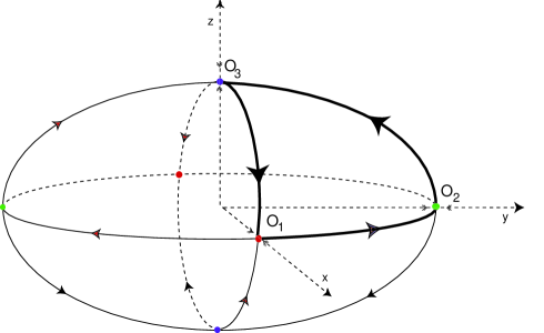
Figure 1. May and Leonard network. Schematic flow of (1.1) for $\gamma=0$. In bold, it is stressed the cycle $\Gamma_{1}$, the restriction of the network to the first octant.

Guckenheimer and Holmes [12] studied a $\Theta$-equivariant vector field, where $\Theta\subset\mathbb{O}(3)$ is the finite Lie group generated by:

$$\ell(x,y,z)=(y,z,x)$$

and

$$k_{1}(x,y,z)=(-x,y,z),\qquad k_{2}(x,y,z)=(x,-y,z),\qquad k_{3}(x,y,z)=(x,y,-z),$$

whose action on ${\mathbb{R}}^{3}$ is isomorphic to ${\mathbb{Z}}_{3}\dot{\ltimes}{\mathbb{Z}}^{2}_{3}$. The coordinate planes and axes are flow-invariant; they correspond to $\text{Fix}\,\,{\mathbb{Z}}_{2}(k_{1})$, $\text{Fix}\,\,{\mathbb{Z}}_{2}(k_{2})$ and $\text{Fix}\,\,{\mathbb{Z}}_{2}(k_{3})$ and their (mutual) intersections. The Birkhoff normal form of a $\Theta$-equivariant vector field at the origin, truncated at order 3, has the form:

$$\left\{\begin{array}[]{l}\dot{x}=x(\lambda+a_{1}x^{2}+a_{2}y^{2}+a_{3}z^{2})\\ \\ \dot{y}=y(\lambda+a_{1}y^{2}+a_{2}z^{2}+a_{3}x^{2})\\ \\ \dot{z}=z(\lambda+a_{1}z^{2}+a_{2}x^{2}+a_{3}y^{2})\end{array}\right.$$ (1.2)

where $a_{1},a_{2},a_{3}\in{\mathbb{R}}$ and $\lambda\in{\mathbb{R}}^{+}$. System (1.2) is related to the May-Leonard system (1.1) with $\gamma=0$, via the change of variables:

$$\overline{x}\mapsto x^{2},\qquad\overline{y}\mapsto y^{2}\qquad\text{and}\qquad\overline{z}\mapsto z^{2}.$$

To convert (1.2) into (1.1) it is also necessary to carry out a rescaling of time and variables $a_{1}$, $\lambda$, in order to set $\lambda=a_{1}=1$.

Variational Matrix	Eigenvalues	Eigenvectors
$Df_{0}(\pm O_{1})=\left(\begin{array}[]{ccc}\displaystyle-1&\displaystyle-1-c\displaystyle&e-1\\ \\ \displaystyle 0&\displaystyle e&\displaystyle 0\\ \\ 0&\displaystyle 0&\displaystyle-c\end{array}\right)$	$\begin{array}[]{c}\displaystyle e\\ \\ -1\\ \\ -c\\ \\ \end{array}$	$\begin{array}[]{cl}\displaystyle\hfil&\displaystyle\left(\frac{1+c}{1+e},-1,0\right)\\ &\\ \displaystyle\hfil&\displaystyle\left(1,0,0\right)\\ &\\ \displaystyle\hfil&\displaystyle\left(\frac{e-1}{1-c},0,1\right)\\ &\\ \end{array}$
$Df_{0}(\pm O_{2})=\left(\begin{array}[]{ccc}\displaystyle-c&\displaystyle 0\displaystyle&0\\ \\ \displaystyle e-1&\displaystyle-1&\displaystyle-1-c\\ \\ 0&\displaystyle 0&\displaystyle e\end{array}\right)$	$\begin{array}[]{c}\displaystyle e\\ \\ -1\\ \\ -c\\ \\ \end{array}$	$\begin{array}[]{cl}\displaystyle\hfil&\displaystyle\left(0,\frac{1+c}{1+e},-1\right)\\ &\\ \displaystyle\hfil&\displaystyle\left(0,1,0\right)\\ &\\ \displaystyle\hfil&\displaystyle\left(1,\frac{e-1}{1-c},0\right)\\ &\\ \end{array}$
$Df_{0}(\pm O_{3})=\left(\begin{array}[]{ccc}\displaystyle e&\displaystyle 0\displaystyle&0\\ \\ \displaystyle 0&\displaystyle-c&\displaystyle 0\\ \\ 1+c&\displaystyle 0&\displaystyle-1\end{array}\right)$	$\begin{array}[]{c}\displaystyle e\\ \\ -1\\ \\ -c\\ \\ \end{array}$	$\begin{array}[]{cl}\displaystyle\hfil&\displaystyle\left(-1,0,\frac{1+c}{1+e}\right)\\ &\\ \displaystyle\hfil&\displaystyle\left(0,0,1\right)\\ &\\ \displaystyle\hfil&\displaystyle\left(0,1,\frac{e-1}{1-c}\right)\\ &\\ \end{array}$

Table 1. Variational matrices, eigenvalues and eigendirections associated to the six equilibria $\pm O_{1}$, $\pm O_{2}$ and $\pm O_{3}$ of (1.1) for $\gamma=0$.

Dynamics for the May-Leonard system

Based on [12, 23], there exists an open set of parameters satisfying (C1a) for which there is an invariant two-dimensional sphere which attracts all trajectories, except the origin. As illustrated in Figure 1, the intersection of this sphere with the axes gives rise to six saddle-type equilibria, say

$$\pm O_{1}\mapsto(\pm 1,0,0),\qquad\pm O_{2}\mapsto(0,\pm 1,0)\qquad\text{and}\qquad\pm O_{3}\mapsto(0,0,\pm 1),$$

whose radial, contracting and expanding eigenvalues/eigendirections are described in Table 1. The formal definition of radial, contracting and expanding eigenvalue/eigendirection may be found in [5, 23] for instance.

The intersection of the sphere with the coordinate planes ${\text{Fix}}\,{\mathbb{Z}}_{2}(k_{i})$ for $i=1,2,3$, generates one-dimensional heteroclinic connections linking the equilibria. The union of these equilibria and connections forms a heteroclinic network that will be denoted by $\Gamma$. The set $\Gamma$ is the union of eight heteroclinic cycles, each one lying on the boundary of each octant. The two-dimensional coordinate subspaces are flow-invariant and prevent visits to more than one cycle in the network. The parameters $e$ and $c$ of (1.1) have been chosen in such a way that the network is asymptotically stable.

The unstable manifolds of the saddles (lying in the closure of the first octant) are given by:

$$W^{u}(+O_{1})\subset\{(x,y,z)\in{\mathbb{R}}^{3}:\quad z=0\quad\wedge\quad x\geq 0\},$$

$$W^{u}(+O_{2})\subset\{(x,y,z)\in{\mathbb{R}}^{3}:\quad x=0\quad\wedge\quad y\geq 0\},$$

and

$$W^{u}(+O_{3})\subset\{(x,y,z)\in{\mathbb{R}}^{3}:\quad y=0\quad\wedge\quad z\geq 0\}.$$

The constant $\delta=c/e>1$ measures the strength of attraction of each cycle in the absence of perturbations. There are no periodic solutions for the case $\delta>1$: typical trajectories starting near $\Gamma$ (but not within $\Gamma$) approach closer and closer one of the cycles in the network and remain near the equilibria for increasing periods of time. These trajectories make fast transitions from one equilibrium point to the next.

The network $\Gamma$ is robust due to a biological constraint: if a species is extinct at time $t=t_{0}$, it will remain extinct for all $t>t_{0}$, $t_{0}\in{\mathbb{R}}_{0}^{+}$. Within each of the invariant planes defined by $x=0$, ${y=0}$ and ${z=0}$, the relevant connecting orbit is a saddle-sink connection, and therefore the network is structurally stable.

In the remaining analysis, we concentrate our attention on the cycle $\Gamma_{1}$:

$$\Gamma_{1}=\Gamma\cap\{(x,y,z)\in{\mathbb{R}}^{3}:\quad x\geq 0,\quad y\geq 0,\quad z\geq 0\}.$$

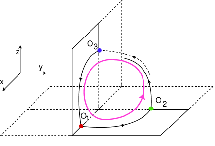
Figure 2. General constant perturbations result in long-period periodic solutions that lie close to the original cycle $\Gamma_{1}$.

As suggested by Figure 2, general symmetry-breaking constant perturbations to (1.1) are well known to result in long-period attracting periodic solutions that lie close to the original cycle. Note that, for $\gamma>0$, the planes defined by the equations $y=0$ and $z=0$ remain flow-invariant and, when restricted to the unit sphere, the periodic forcing is non-negative.

Terminology

For future use, we settle the following notation:

$$\displaystyle a_{1} = \frac{c^{2}}{c^{2}+4\omega^{2}}\qquad\qquad\displaystyle a_{2}=\frac{e^{2}}{e^{2}+4\omega^{2}}$$

$$b_{1} = \frac{2\,c\,\omega}{c^{2}+4\omega^{2}}\qquad\qquad\displaystyle b_{2}=\frac{2\,e\,\omega}{e^{2}+4\omega^{2}}$$

$$\xi = \frac{e^{2}+ce+c^{2}}{e^{3}}\quad\qquad\delta=c/e$$

2. Main result and framework of the article

Let $\mathcal{T}$ be a tubular neighborhood of the May-Leonard network $\Gamma$, which exists for system (1.1) with $\gamma=0$. We define a cross-section $\Sigma$ to which all trajectories in $\mathcal{T}$ intersect transversely. For $\gamma\geq 0$, repeated intersections define a subset $\mathcal{D}\subset\Sigma$ where the return map to $\mathcal{D}$ is well defined. Under Hypotheses (C1a) and (C1b), we may obtain an approximation of the first return map reduced to the leading phase coordinate. As well as the values of the coordinates, the non-autonomous nature of the dynamics requires us to keep track of the elapsed time spent on each part of the trajectory.

From now on, let us denote by $\mathcal{F}_{\gamma}$ the map which comprises the leading phase coordinate of the first return map and the elapsed time. The detailed construction of this map, as well the topology of the approximation, may be found in Section 3. The novelty of this article is the following result:

Theorem A.

For $\omega>0$ sufficiently small, there exists $\xi^{\star}>0$ such that for all $\xi>\xi^{\star}$ the following inequality holds:

$$\liminf_{r\rightarrow 0^{+}}\,\,\frac{\emph{Leb}\left\{\gamma\in[0,r]:\mathcal{F}_{\gamma}\text{ exhibits a strange attractor with a SRB measure}\right\}}{r}>0.$$

where Leb denotes the one-dimensional Lebesgue measure.

The existence of a set with positive lower Lebesgue density at 0 for which we observe strange attractors justifies the title of this manuscript. These strange attractors and SRB measures have strong statistical properties that will be made precise in Sections 4 and 6. The proof of Theorem A is performed in Section 6 by reducing the analysis of the two-dimensional map $\mathcal{F}_{\gamma}$ to the dynamics of a one-dimensional map, via the Theory of rank-one attractors.

Numerical evidences

The existence of non-hyperbolic strange attractors has been suggested by the numerics presented by J. Dawes and T.-L. Tsai [9, 25, 26] when $\omega\approx 0$ and $\delta\gg 1$, namely:

1. the existence of $n$ periodic orbits, apparently for all natural numbers $n$;

2. the maximum return times of orbits appears to increase without an upper bound;

3. the test for chaos developed by Gottwald and Melbourne [10] indicates the presence of chaos;

4. the existence of non-trivial rotation intervals [16].

Structure of the paper

The rest of this article is organised as follows: in Section 3, we state all results related to the topic and we explain how Theorem A fits in the literature. The proof of this result is performed using the Theory of rank-one attractors, whose basic ideas are explained in Section 4. In Section 5, we refine some results used to prove the main theorem in Section 6. We point out some bifurcations in the family of vector fields (1.1) in Section 7, emphasising the role of the parameter $\xi$. Section 8 concludes this article with a discussion. Throughout this paper, we have endeavoured to make a self contained exposition bringing together all topics related to the proofs. We have drawn illustrative figures to make the paper easily readable.

3. Overview

For completeness, we give a complete overview on the subject of the article and we explain how our result fits in the literature. The main results on the topic are summarised in Table  3. In what follows, we use the terminology defined at the beginning of Section 2.

For $\gamma\geq 0$, the return map to a cross section $\Sigma$ of $f_{\gamma}$ depends on the phase space and on the initial time. The next theorem yields a description of a map that comprises the leading component of the first return map and the return time $s$ at which orbits reach the cross section:

Theorem 3.1 ([2, 26], adapted).

For $\gamma\geq 0$, there is $\tilde{\varepsilon}>0$ (small) such that a solution of (1.1) that starts in $\Sigma$ at time $s$, returns to $\Sigma$ with the dynamics dominated by the coordinate $x$, defining a map on the cylinder

$$(x,s)\in\mathcal{D}:=\{x/\tilde{\varepsilon}\in\,\,]\,0,1]\quad\text{and}\quad s\in{\mathbb{R}}\pmod{\pi/\omega}\},$$

that is approximated, in the $C^{3}$–Whitney topology, by:

$$\mathcal{F}_{\gamma}(x,s)=(\mathcal{F}^{1}_{\gamma}(x,s),\mathcal{F}^{2}_{\gamma}(x,s)\pmod{\pi/\omega})$$ (3.1)

with

$$\mathcal{F}^{1}_{\gamma}(x,s) = \mu x^{\delta}+\gamma[\mu_{1}+\mu_{2}(-a_{1}\cos(2\omega\Phi(x,s))-b_{1}\sin(2\omega\Phi(x,s))$$

$$-\mu_{4}(-a_{1}\cos(2\omega(\mathcal{F}^{2}_{\gamma}(x,s)-\Delta_{3}))-b_{1}\sin(2\omega(\mathcal{F}^{2}_{\gamma}(x,s)-\Delta_{3})))$$

$$-\mu_{5}(-a_{2}\cos(2\omega\mathcal{F}^{2}_{\gamma}(x,s))-b_{2}\sin(2\omega\mathcal{F}^{2}_{\gamma}(x,s)))]+\mathcal{O}(\gamma^{2}),$$

$$\mathcal{F}^{2}_{\gamma}(x,s) = s+\mu_{3}-\xi\log(x)-\frac{\gamma\,\xi}{e\,x}[\eta_{\omega}(x,s)-a_{2}\cos(2\omega s)+b_{2}\sin(2\omega s)]+\mathcal{O}(\gamma^{2}),$$

where

$$\Phi(x,s)=s+\mu_{3}-\xi\log(x),\qquad\eta_{\omega}(x,s)=\frac{e^{2}\cos^{2}(\omega s)+2\omega^{2}}{(e^{2}+4\omega^{2})}$$

and $\mu_{1},\mu_{2},\mu_{3},\mu_{4},\mu_{5}\in{\mathbb{R}},\,\,\Delta_{3}\in{\mathbb{R}}^{+}$ depend on the transition maps.

The map $\eta_{\omega}$ does not depend on $x$. The amplitude $\gamma$ of the periodic forcing is sufficiently small so that the $\mathcal{O}(\gamma^{2})$–terms are neglected, where $\mathcal{O}$ denotes the standard Landau notation. The proof of Theorem 3.1 is partially performed in [26] by composing local and transition maps around the equilibria. We say “partially” because the authors used a linearisation form which, in principle, is valid just in the $C^{1}$–topology. In §5.2, using results by Wang and Ott [28], we revisit the computation of $\mathcal{F}_{\gamma}$ in a $C^{3}$–controlled manner.

For $\gamma>0$, we distinguish four dynamical regimes for (1.1), which depend subtly on the following parameters in the problem: the saddle-value $\delta$, the frequency $\omega$ of the non-autonomous periodic perturbation and a constant $\mu_{1}$ that depends on the global parts of the dynamics. The four regimes, summarised in Table 2, are:

Case 1:

$\delta\gtrsim 1$ and $\omega\approx 0$,

Case 2:

$\delta\gg 1$ and $\omega\approx 0$,

Case 3:

$\xi<{2\mu_{1}}$ and $\omega\gg 0$,

Case 4:

$\xi>{2\mu_{1}}$ and $\omega\gg 0$.

Parameters	$\delta\gtrsim 1$	$\delta\gg 1$
$\omega\approx 0$	Case 1	Case 2
Parameters	$\xi<{2\mu_{1}}$	$\xi>{2\mu_{1}}$
$\omega\gg 0$	Case 3	Case 4

Table 2. Four different cases for the dynamics of (3.1).

The meaning of the terminology suggested by [26] is the following. Without causing qualitative changes in the bifurcation structure:

• $\mathbf{\delta\gtrsim 1}$ means that, for a given $\gamma>0$, $\delta$ is such that $\gamma^{\delta-1}\approx 1$ and thus the term $\mu x^{\delta}$ cannot be omitted from the expression of $\mathcal{F}^{1}_{\gamma}$;
  

• $\mathbf{\delta\gg 1}$ means that, for a given $\gamma>0$, $\delta$ is so large that $\gamma^{\delta-1}\approx 0$ and thus the term $\mu x^{\delta}$ may be ignored from the expression of $\mathcal{F}^{1}_{\gamma}$;
  

• $\mathbf{\omega\approx 0}$ means that the value of $\omega$ is so small that $b_{1}$ and $b_{2}$ may be ignored from $\mathcal{F}^{1}_{\gamma}$;
  

• $\mathbf{\omega\gg 0}$ means that the value of $\omega$ is so large that ${a_{1}},a_{2},b_{1}$ and $b_{2}$ may be approximated by 0 in $\mathcal{F}^{1}_{\gamma}$.
  

A clarification of this notation will be clearer in §5.1. In what follows, we describe the expression of $\mathcal{F}_{\gamma}$ for each of the previous cases and the associated dynamics.

3.1. Cases 1 and 2

In Cases 1 and 2, we have $\omega\approx 0$, which implies that $b_{1}$ and $b_{2}$ vanish and $a_{1}$ and $a_{2}$ are close to 1 (cf. §5.1). For $\delta>1$, $\mathcal{F}_{\gamma}$–iterates lie close to an invariant curve that may be well approximated by:

$$\mu x^{\delta}+\gamma\mu_{1}\left[1-\sqrt{a_{1}}\cos(2\omega\Psi(x,s))\right]$$ (3.2)

where $\sqrt{a_{1}}<1$, $\Psi:\mathcal{D}\rightarrow{\mathbb{R}}$ is $C^{3}$–smooth and $1-\sqrt{a_{1}}\cos(2\omega\Psi(0,s))$ is a Morse function with finitely many non-degenerate critical points. Although all the theory is valid for a more general map, we assume hereafter that:

(C2):

$\Psi(x,s)=s$.

Comparisons with numerics of [9, 25, 26] show that the model (3.2), under Hypothesis (C2), is sufficient to capture the dynamics. This is the reason why we assume, from now on, that these conditions are verified. Therefore, we may rewrite Theorem 3.1 (with $\mu=1$) as:

Proposition 3.2.

For $\gamma\geq 0$, there is $\tilde{\varepsilon}>0$ such that a solution of (1.1) that starts in $\Sigma$ at time $s$, returns to $\Sigma$ with the dynamics dominated by the coordinate $x$, defining a map on the cylinder

$$(x,s)\in\tilde{\mathcal{D}}:=\{x/\tilde{\varepsilon}\in\,\,]\,0,1]\quad\text{and}\quad s\in{\mathbb{R}}\pmod{1}\},$$

that is approximated, in the $C^{3}$–Whitney topology, by:

$$\mathcal{F}_{\gamma}(x,s)=(\mathcal{F}^{1}_{\gamma}(x,s)\,,\,\mathcal{F}^{2}_{\gamma}(x,s))$$

where:

$$\left\{\begin{array}[]{l}\mathcal{F}^{1}_{\gamma}(x,s)=x^{\delta}+\gamma\mu_{1}(1-\sqrt{a_{1}}\cos(2\pi s))\\ \\ \mathcal{F}^{2}_{\gamma}(x,s)=\displaystyle s+\frac{\mu_{3}\omega}{\pi}-\displaystyle\frac{\xi\omega}{\pi}\log(x^{\delta}+\gamma\mu_{1}(1-\sqrt{a_{1}}\cos(2\pi s)))+\mathcal{O}(\gamma)\pmod{1}\\ \end{array}\right.$$ (3.3)

A clarification of the expression of $\mathcal{F}^{2}_{\gamma}$ is given in §5.4. For $\delta>1$ and $\gamma>0$ small, the map $x\mapsto x^{\delta}+\gamma$ has two fixed points. In what follows, let us denote by ${x}^{\star}$ its positive stable fixed point, as stressed in Figure 3.

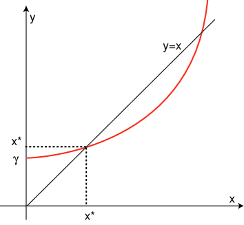
Figure 3. For $\delta>1$ and $\gamma>0$, the map $x\mapsto x^{\delta}+\gamma$ has two fixed points. The symbol $x^{\star}$ denotes the positive stable fixed point.

Theorem 3.3 (Case 1, [2, 26], adapted).

If $\delta>1$ and $\gamma>0$ are such that ${x}^{\star}>\gamma$, there exists $\omega_{0}>0$ such that for all $\omega\in\,\,]\,0,\omega_{0}\,[$, the system (3.3) has an invariant closed curve as its maximal attractor.

Under the conditions of Theorem 3.3, for $\omega\in\,\,]\,0,\omega_{0}\,[$ fixed, if $\xi$ is sufficiently large, then the closed curve may break and saddle-node and period-doubling bifurcations may occur. This is implicit in [26]. The dynamics of Case 1 alternates between an invariant curve and saddle-node bifurcations, giving rise to bistability dynamics for (3.3): coexistence of a stable fixed point and a stable invariant curve (cf. Region III of [25]).

Theorem 3.4 (Case 2, [2], adapted).

For $\gamma>0$ sufficiently small and $C>2$, if

$$\frac{\exp(C/\xi\omega)-1}{\exp(C/\xi\omega)-1/C}<\sqrt{a_{1}}<1$$

then there exists a hyperbolic invariant closed set $\Lambda$ such that the dynamics of $\mathcal{F}_{\gamma}|_{\Lambda}$ is topologically conjugate to the Bernoulli shift on two symbols.

The set $\Lambda$ is hyperbolic and topologically transitive. Since $\mathcal{F}_{\gamma}$ is $C^{2}$, this class of objects has zero Lebesgue measure. Theorem A of this article gives a conclusive analytical result, ensuring that the flow of (3.3) exhibits observable and persistent chaotic dynamics in Case 2. When $\delta\gg 1$ ($\Rightarrow\xi\gg 1$), the dynamics is chaotic for $\omega\gtrsim 0$ [25].

3.2. Cases 3 and 4

Proposition 3.5.

For $\gamma\geq 0$, there is $\tilde{\varepsilon}>0$ such that a solution of (1.1) that starts in $\Sigma$ at time $s$, returns to $\Sigma$ with the dynamics dominated by the coordinate $x$, defining a map on the cylinder $\tilde{\mathcal{D}}$ that is approximately given by

$$\mathcal{F}_{\gamma}(x,s)=(\mathcal{F}^{1}_{\gamma}(x,s)\,,\,\mathcal{F}^{2}_{\gamma}(x,s))$$

where:

$$\left\{\begin{array}[]{l}\mathcal{F}^{1}_{\gamma}(x,s)=\gamma\,\mu_{1}\\ \\ \mathcal{F}^{2}_{\gamma}(x,s)=\displaystyle s+\frac{\mu_{3}\,\omega}{\pi}-\frac{\xi\,\omega}{\pi}\log(\gamma\,\mu_{1})-\frac{\xi\,\omega}{2\,e\,\pi\,\mu_{1}}+\frac{\xi}{2\,\pi\,\mu_{1}}\sin(2\pi s)\pmod{1}\\ \end{array}\right.$$ (3.4)

A clarification for the expression of $\mathcal{F}^{2}_{\gamma}$ is given in Subsection 5.5. The next result shows that the dynamics of $\mathcal{F}_{\gamma}$ for Cases 3 and 4 are governed by the canonical family of circle maps [8].

Theorem 3.6 (Cases 3 and 4, [26]).

If $\xi<{2\mu_{1}}$, then system (3.4) is equivalent to the canonical family of invertible circle maps; otherwise, if $\xi>{2\mu_{1}}$, then system (3.4) is equivalent to the canonical family of non-invertible circle maps.

Rotation numbers (associated to a circle map) form a closed subset of $[0,1]$ and, for monotone maps, it can be shown that the rotation number is unique and independent of the choice of initial condition $s_{0}\in{\mathbb{R}}$. Non-invertible circle maps of the type of (3.4) with $\xi>{2\mu_{1}}$ suggest more complicated dynamics since an interval of rotation numbers may exist [8]. For any rotation number within the rotation interval, there exists an initial point $s_{0}$ whose orbit has that rotation number. Since orbits are periodic if and only if they have rational rotation numbers, the existence of a rotation interval implies the existence of countably many periodic orbits at that parameter value. Thus, the existence of a non-trivial rotation interval for (3.4) implies chaos in the sense of [16].

Parameters	$\delta\gtrsim 1$	$\delta\gg 1$
	Case 1	Case 2
$\omega\approx 0$	Attracting two-torus	Hyperbolic horseshoes [2]
	[2, 25, 26]	Strange attractors (New)
Parameters	${\xi}<{2\mu_{1}}$	${\xi}>{2\mu_{1}}$
	Case 3	Case 4
$\omega\gg 0$	Invertible two-torus	Non-invertible two-torus
	[9, 25, 26]	[9, 25, 26]

Table 3. Overview of the results in the literature and the contribution of the present article (in blue) for the equation (1.1).

4. Theory of rank-one maps in two-dimensions

We gather in this section a collection of technical facts used repeatedly in later sections. In what follows, let us denote by $C^{2}({\mathbb{S}}^{1},{\mathbb{R}})$ the set of $C^{2}$–maps from ${\mathbb{S}}^{1}$ (unit circle) to ${\mathbb{R}}$.

4.1. Misiurewicz-type map

We say that $h\in C^{2}({\mathbb{S}}^{1},{\mathbb{R}})$ is a Misiurewicz map if the following hold for some neighborhood $U$ of the critical set $C=\{x\in{\mathbb{S}}^{1}:h^{\prime}(x)=0\}$.

1. (Outside $U$) There exist $\lambda_{0}>0$, $M_{0}\in{\mathbb{N}}$, and $0<d_{0}\leq 1$ such that:

   1. for all $m\geq M_{0}$, if $h^{i}(x)\notin U$ for all $0\leq i\leq m-1$, then $|(h^{m})^{\prime}(x)|\geq\exp(\lambda_{0}m)$.

   2. for all $m\in{\mathbb{N}}$, if if $h^{i}(x)\notin U$ for all $0\leq i\leq m-1$ and $h^{m}(x)\in U$, then $|(h^{m})^{\prime}(x)|\geq d_{0}\,\exp(\lambda_{0}m)$.

2. (Critical orbits) For all $c\in C$ and $i>0$, $h^{i}(c)\notin U$.

3. (Inside $U$)

   1. $h^{\prime\prime}(x)\neq 0$ for all $x\in U$ and

   2. for all $x\in U\backslash C$, there exists $p_{0}(x)\in{\mathbb{N}}$ such that $h^{i}(x)\notin U$ for all $i<p_{0}(x)$ and $\left|\left(h^{p_{0}(x)}\right)^{\prime}(x)\right|\geq\displaystyle\frac{\exp(\lambda_{0}p_{0}(x)/3)}{d_{0}}$

These types of maps are a slight generalization of the maps studied by Misiurewicz [18]. The property “to be a Misiurewicz map” is not an open condition, i.e. it does not persist form small smooth perturbations.

4.2. Rank-one maps

The theory of chaotic rank-one attractors has been originated from the theory of Benedicks and Carleson on Hénon strange attractors [7] and the development that followed by Young and Benedicks [33]. This theory grew and has been generalised by Young and Wang in a sequence of articles [29, 30, 31, 32].

Let $M=[0,1]\times{\mathbb{S}}^{1}$ with the usual topology. We consider the two-parametric family of maps $F_{(a,b)}:M\rightarrow M$, where $a\in[0,1]$ and $b\in{\mathbb{R}}$ is a scalar. Let $B_{0}\subset{\mathbb{R}}\backslash\{0\}$ with $0$ as an accumulation point. Rank-one theory states the following:

(H1) Regularity conditions:

1. For each $b\in B_{0}$, the function $(x,s,a)\mapsto F_{(a,b)}$ is at least $C^{3}$–smooth.

2. Each map $F_{(a,b)}$ is an embedding of $M$ into itself.

3. There exists $k\in{\mathbb{R}}^{+}$ independent of $a$ and $b$ such that for all $a\in[0,1]$, $b\in B_{0}$ and $(x_{1},s_{1}),(x_{2},s_{2})\in M$, we have:

   $$\frac{|\det DF_{(a,b)}(x_{1},s_{1})|}{|\det DF_{(a,b)}(x_{2},s_{2})|}\leq k.$$

(H2) Existence of a singular limit:

For $a\in[0,1]$, there exists a map

$$F_{(a,0)}:M\rightarrow{\mathbb{S}}^{1}\times\{0\}$$

such that the following property holds: for every $(x,s)\in M$ and $a\in[0,1]$, we have

$$\lim_{b\rightarrow 0}F_{(a,b)}(x,s)=F_{(a,0)}(x,s).$$

(H3) $C^{3}$–convergence to the singular limit:

For every choice of $a\in[0,1]$, the maps $(x,y,a)\mapsto F_{(a,b)}$ converge in the $C^{3}$–topology to $(x,y,a)\mapsto F_{(a,0)}$ on $M\times[0,1]$ as $b$ goes to zero.

(H4) Existence of a sufficiently expanding map within the singular limit:

There exists $a^{\star}\in[-\varepsilon,\varepsilon]$ such that $h_{a^{\star}}(s)=F_{(a^{\star},0)}(0,s)$ is a Misiurewicz-type map (see Subsection 4.1 and Remark 4.1).

(H5) Parameter transversality:

Let $C_{a^{\star}}$ denote the critical set of a Misiurewicz-type map $h_{a^{\star}}$ (see Subsection 4.1). For each $s\in C_{a^{\star}}$, let $p=h_{a^{\star}}(x)$, and let $\widetilde{s(a)}$ and $\widetilde{p(a)}$ denote the continuations of $s$ and $p$, respectively, as the parameter $a$ varies around $a^{\star}$. The point $\widetilde{p(a)}$ is the unique point such that $\widetilde{p(a)}$ and $p$ have identical symbolic itineraries under $h_{a^{\star}}$ and $h_{\tilde{a}}$, respectively. We have:

$$\frac{d}{da}h_{\tilde{a}}(s(\widetilde{a}))|_{a=a^{\star}}\neq\frac{d}{da}p(\tilde{a})|_{a=a^{\star}}.$$

(H6) Nondegeneracy at turns:

For each $s\in C_{a^{\star}}$ (set of critical points of $h_{a^{\star}}$), we have

$$\frac{d}{ds}F_{(a^{\star},0)}(x,s)|_{x=0}\neq 0.$$

(H7) Conditions for mixing:

If $J_{1},\ldots,J_{r}$ are the intervals of monotonicity of the Misiurewicz-type map $h_{a^{\star}}(s)=F_{(a^{\star},0)}(0,s)$, then:

1. $\exp(\lambda_{0}/3)>2$ (see the meaning of $\lambda_{0}$ in Subsection 4.1) and

2. if $Q=(q_{im})$ is the matrix of all possible transitions defined by:

   $$\left\{\begin{array}[]{l}1\qquad\text{if}\qquad J_{m}\subset h_{a^{\star}}(J_{i})\\ 0\qquad\text{otherwise},\\ \end{array}\right.$$

   then there exists $N\in{\mathbb{N}}$ such that $Q^{N}>0$ (i.e. all entries of the matrix $Q^{N}$, endowed with the usual product, are positive).

Remark 4.1.

Identifying $\{0\}\times{\mathbb{S}}^{1}$ with ${\mathbb{S}}^{1}$, we refer to $F_{(a,0)}$ the circle map $h_{a}:{\mathbb{S}}^{1}\rightarrow{\mathbb{S}}^{1}$ defined by $h_{a}(s)=F_{(a,0)}(0,s)$ as the singular limit of $F_{(a,b)}$.

4.3. Strange attractors and SRB measures

Following [30], we formalize the notion of strange attractor supporting an ergodic SRB measure, for a two-parametric family $F_{(a,b)}$ defined on the set $M=[0,1]\times{\mathbb{S}}^{1}$, endowed with the induced topology. In what follows, if $A\subset M$, let us denote by $\overline{A}$ its topological closure.

Let $F_{(a,b)}$ be an embedding such that $F_{(a,b)}(\overline{U})\subset U$ for some open set $U\subset M$. In the present work we refer to

$${\Omega}=\bigcap_{m=0}^{+\infty}F_{({a},b)}^{m}(\overline{U}).$$

as an attractor and $U$ as its basin. The attractor $\Omega$ is irreducible if it cannot be written as the union of two (or more) disjoint attractors.

Definition 3.

We say that $F_{({a},b)}$ possesses a strange attractor supporting an ergodic SRB measure $\nu$ if:

• for Lebesgue almost all $(x,s)\in U$, the $F_{({a},b)}$–orbit of $(x,s)$ has a positive Lyapunov exponent, i.e.

  $$\lim_{n\in{\mathbb{N}}}\frac{1}{n}\|DF_{({a},b)}^{n}(x,s)\|>0;$$

• $F_{({a},b)}$ admits a unique ergodic SRB measure (with no-zero Lyapunov exponents);

• for Lebesgue almost all points $(x,s)\in U$ and for every continuous function $\varphi:U\rightarrow{\mathbb{R}}$, we have:

  $$\lim_{n\in{\mathbb{N}}}\quad\frac{1}{n}\sum_{i=0}^{n-1}\varphi\circ F_{({a},b)}^{i}(x,s)=\int\varphi\,d\nu.$$ (4.1)

Admitting that $F_{({a},b)}$ admits a unique ergodic SRB measure $\nu$, we define convergence of $F_{({a},b)}$ with respect to $\nu$.

Definition 4.

We say that:

• $F_{({a},b)}$ converges (in distribution with respect to $\nu$) to the normal distribution if, for every Holder continuous function $\varphi:U\rightarrow{\mathbb{R}}$, the sequence $\left\{\varphi\left(F_{(\tilde{a},b)}^{i}\right):i\in{\mathbb{N}}\right\}$ obeys a central limit theorem; in other words, if $\int\varphi\,d\nu=0$, then the sequence

  $$\frac{1}{\sqrt{m}}\sum_{i=0}^{m-1}\varphi\circ F_{(\tilde{a},b)}^{i}$$

  converges in distribution (with respect to $\nu$) to the normal distribution.
  

• the pair $(F_{({a},b)},\nu)$ is mixing if it is isomorphic to a Bernoulli shift.

4.4. Q. Wang and L.-S. Young’s reduction

The results developed in [29, 30, 31, 32] are about maps with attracting sets on which there is strong dissipation and (in most places) a single direction of instability. Two-parameter families ${F_{(a,b)}}$ have been considered and it has been proved that if a singular limit makes sense (for $b=0$) and if the resulting family of 1D maps has certain “good” properties, then some of them can be passed back to the two-dimensional system ($b>0$). They allow us to prove results on strange attractors for a positive Lebesgue measure set of $a$.

For attractors with strong dissipation and one direction of instability, Wang and Young conditions (H1)–(H7) are simple and checkable; when satisfied, they guarantee the existence of strange attractors with a package of statistical and geometric properties:

Theorem 4.2 ([30], adapted).

Suppose that the two-parametric family of maps $F_{(a,b)}$ satisfies (H1)–(H7). Then, for all sufficiently small $b\in B_{0}$, there exists a subset $\Delta\in[-\varepsilon,\varepsilon]$ with positive Lebesgue measure such that for all $a\in\Delta$, the map $F_{({a},b)}$ admits an irreducible strange attractor $\tilde{\Omega}\subset\Omega$ that supports a unique ergodic SRB measure $\nu$. The orbit of Lebesgue almost all points in $\tilde{\Omega}$ is asymptotically distributed according to $\nu$. Furthermore, $(F_{({a},b)},\nu)$ is mixing.

In contrast to earlier results, the theory in [29, 30, 31, 32] is generic, in the sense that the conditions under which it holds rely only to certain general characteristics of the maps and not to specific formulas or contexts.

5. Preparatory section

In this section, we put together some preliminaries needed for the proof of Theorem A. We start by listing some properties of the constants which appear in the expression of $\mathcal{F}_{\gamma}$. Then, in §5.2, we refine the expression of $\mathcal{F}_{\gamma}$ in the four cases under consideration.

5.1. Control of variables

In this section, we present additional information about the constants which appear in the expression of $\mathcal{F}_{\gamma}$. We set $a_{1},a_{2},b_{1},b_{2}$ as real valued functions on $\omega\geq 0$.

Lemma 5.1.

The following equalities are valid:

1. $a_{1}^{2}+b_{1}^{2}=a_{1}$ and $a_{2}^{2}+b_{2}^{2}=a_{2}$.
   

2. $\displaystyle\lim_{\omega\rightarrow 0}a_{1}(\omega)=\lim_{\omega\rightarrow 0}a_{2}(\omega)=1$   and   $\displaystyle\lim_{\omega\rightarrow 0}b_{1}(\omega)=\lim_{\omega\rightarrow 0}b_{2}(\omega)=0$.
   

3. $\displaystyle\lim_{\omega\rightarrow+\infty}a_{1}(\omega)=\lim_{\omega\rightarrow+\infty}a_{2}(\omega)=\lim_{\omega\rightarrow+\infty}b_{1}(\omega)=\lim_{\omega\rightarrow+\infty}b_{2}(\omega)=0$.
   

4. $\displaystyle c\,\xi=\delta(1+\delta+\delta^{2})$   and   $\displaystyle e\,\xi=(1+\delta+\delta^{2})$.
   

5. $\displaystyle\lim_{\omega\rightarrow+\infty}\left[\sqrt{a_{2}(\omega)}\big{/}\frac{e}{2\omega}\right]=1$   and   $\displaystyle\lim_{\omega\rightarrow+\infty}\left[\sqrt{a_{2}(\omega)}-\frac{e}{2\omega}\right]=0$.
   

6. $\displaystyle\lim_{\omega\rightarrow+\infty}\left[b_{2}(\omega)/a_{2}(\omega)\right]=+\infty$.

Proof.

Taking into account the constants list defined on §1, the proof of this result is quite elementary. For the sake of completeness, we present the proof without deep details.

1. The equalities follow from:

   $$a_{1}^{2}+b_{1}^{2}=\frac{c^{4}}{(c^{2}+4\omega^{2})^{2}}+\frac{4c^{2}\omega^{2}}{(c^{2}+4\omega^{2})^{2}}=\frac{c^{2}(c^{2}+4\omega^{2})}{(c^{2}+4\omega^{2})^{2}}=\frac{c^{2}}{(c^{2}+4\omega^{2})}=a_{1}$$

   and

   $$a_{2}^{2}+b_{2}^{2}=\frac{e^{4}}{(e^{2}+4\omega^{2})^{2}}+\frac{4e^{2}\omega^{2}}{(e^{2}+4\omega^{2})^{2}}=\frac{e^{2}(e^{2}+4\omega^{2})}{(e^{2}+4\omega^{2})^{2}}=\frac{e^{2}}{(e^{2}+4\omega^{2})}=a_{2}.$$

2. It is straightforward to conclude that:

   $$\lim_{\omega\rightarrow 0}a_{1}(\omega)=\lim_{\omega\rightarrow 0}\frac{c^{2}}{c^{2}+4\omega^{2}}=\lim_{\omega\rightarrow 0}\frac{e^{2}}{e^{2}+4\omega^{2}}=\lim_{\omega\rightarrow 0}a_{2}(\omega)=1$$

   and

   $$\lim_{\omega\rightarrow 0}b_{1}(\omega)=\lim_{\omega\rightarrow 0}\frac{2c\omega}{c^{2}+4\omega^{2}}=\lim_{\omega\rightarrow 0}\frac{2e\omega}{e^{2}+4\omega^{2}}=\lim_{\omega\rightarrow 0}b_{2}(\omega)=0.$$

3. By definition, it is clear that:

   $$\lim_{\omega\rightarrow+\infty}a_{1}(\omega)=\lim_{\omega\rightarrow+\infty}\frac{c^{2}}{c^{2}+4\omega^{2}}=\lim_{\omega\rightarrow+\infty}\frac{e^{2}}{e^{2}+4\omega^{2}}=\lim_{\omega\rightarrow+\infty}a_{2}(\omega)=0$$

   and

   $$\lim_{\omega\rightarrow+\infty}b_{1}(\omega)=\lim_{\omega\rightarrow+\infty}\frac{2c\omega}{c^{2}+4\omega^{2}}=\lim_{\omega\rightarrow+\infty}\frac{2e\omega}{e^{2}+4\omega^{2}}=\lim_{\omega\rightarrow+\infty}b_{2}(\omega)=0.$$

4. This item follows from the equalities:

   $$c\xi=\frac{ce^{2}+c^{2}e+c^{3}}{e^{3}}=\frac{c}{e}\left(\frac{e^{2}}{e^{2}}+\frac{c}{e}+\frac{c^{2}}{e^{2}}\right)=\delta(1+\delta+\delta^{2})$$

   and

   $$e\xi=\frac{e^{2}+ce+c^{2}}{e^{2}}=1+\delta+\delta^{2}.$$

5. The item follows from:

   $$\lim_{\omega\rightarrow+\infty}\left[\sqrt{a_{2}(\omega)}\big{/}\frac{e}{2\omega}\right]=\lim_{\omega\rightarrow+\infty}\left[{\frac{2e\omega}{e\,\sqrt{e^{2}+4\omega^{2}}}}\right]=\lim_{\omega\rightarrow+\infty}\left[{\frac{2}{\sqrt{e^{2}/\omega^{2}+4}}}\right]=1$$

   and

   $$\lim_{\omega\rightarrow+\infty}\left[\sqrt{a_{2}(\omega)}-\frac{e}{2\omega}\right]=\lim_{\omega\rightarrow+\infty}\left[\sqrt{\frac{e^{2}}{e^{2}+4\omega^{2}}}-\frac{e}{2\omega}\right]=\lim_{\omega\rightarrow+\infty}\left[\sqrt{\frac{e^{2}/\omega^{2}}{e^{2}/\omega^{2}+4}}-\frac{e}{2\omega}\right]=0.$$

6. It is immediate to check that:

   $$\lim_{\omega\rightarrow+\infty}\left[b_{2}(\omega)/a_{2}(\omega)\right]=\lim_{\omega\rightarrow+\infty}\frac{2\,e\,\omega(e^{2}+4\,\omega^{2})}{e^{2}\,(e^{2}+4\,\omega^{2})}=\lim_{\omega\rightarrow+\infty}\frac{2\,\omega}{e}=+\infty.$$

∎

5.2. First return map

In this subsection, we give an expression for the first return map to a given cross section to $\Gamma$ (at leading order), obtained as the composition of two types of maps: local maps between the neighbourhood walls of the hyperbolic equilibria where we may compute a normal form, and global maps from one neighbourhood wall to another.

5.2.1. Local map

In what follows, we set $i\in\{1,2,3\}$ and $j\in\{s,r,u\}$. Assuming Hypotheses (C1a) and (C1b), according to Wang and Ott [28], there exists $\gamma_{i}>0$ and $V_{i}$, a $\tilde{\varepsilon}_{i}$–cubic neighbourhood of $O_{i}$, where the vector field $f_{\gamma}$, $\gamma\in[0,\gamma_{i}]$ may be written as:

$$\left\{\begin{array}[]{l}\dot{x}_{s}=-c+\gamma\,\,g_{s}(\gamma x_{s},\gamma x_{r},\gamma x_{u},\theta;\gamma)x_{s}\\ \\ \dot{x}_{r}=-1+\gamma\,\,g_{r}(\gamma x_{s},\gamma x_{r},\gamma x_{u},\theta;\gamma)x_{r}\\ \\ \dot{x}_{u}=e+\gamma\,\,g_{u}(\gamma x_{s},\gamma x_{r},\gamma x_{u},\theta;\gamma)x_{u}\\ \\ \dot{\theta}=2\omega\end{array}\right.$$ (5.1)

where

• $\tilde{\varepsilon}_{i}>0$ is small,
  

• $g_{s},g_{r},g_{u}$ are analytic maps in $V_{i}\times{\mathbb{S}}^{1}\times[0,\gamma_{0}]$,
  

• $\|g_{j}\|_{C^{3}}<K_{1}$ for some $K_{1}>0$ ($\|\star\|_{C^{3}}$ denotes the $C^{3}$–norm).

Remark 5.2.

The terminology $s,r,u$ corresponds to the contracting, radial and expanding direction near each equilibrium. The maps $g_{s},g_{r}$ and $g_{u}$ depend on the equilibrium around which the normal form is being calculated.

After rescaling variables

$$x_{s}\mapsto x_{s}/\tilde{\varepsilon}_{i},\qquad x_{r}\mapsto x_{r}/\tilde{\varepsilon}_{i},\qquad x_{u}\mapsto x_{u}/\tilde{\varepsilon}_{i},$$

we may define the cross sections ${\text{In}}(O_{i})$ and ${\text{Out}}(O_{i})$ as follows (see Figure 4):

$${\text{In}}(O_{1}) = \{(x_{s},x_{r},x_{u}):|x_{r}|\leq 1,0\leq x_{u}\leq 1,x_{s}=1\},$$

$${\text{Out}}(O_{1}) = \{(x_{s},x_{r},x_{u}):|x_{r}|\leq 1,x_{u}=1,0\leq x_{s}\leq 1\},$$

$${\text{In}}(O_{2}) = \{(x_{s},x_{r},x_{u}):x_{s}=1,0\leq|x_{r}|\leq 1,0\leq x_{u}\leq 1\},$$

$${\text{Out}}(O_{2}) = \{(x_{s},x_{r},x_{u}):0\leq x_{s}\leq 1,|x_{r}|\leq 1,x_{u}=1\},$$

$${\text{In}}(O_{3}) = \{(x_{s},x_{r},x_{u}):0\leq x_{u}\leq 1,x_{s}=1,|x_{r}|\leq 1\},$$

$${\text{Out}}(O_{3}) = \{(x_{s},x_{r},x_{u}):x_{u}=1,0\leq x_{s}\leq 1,|x_{r}|\leq 1\}.$$

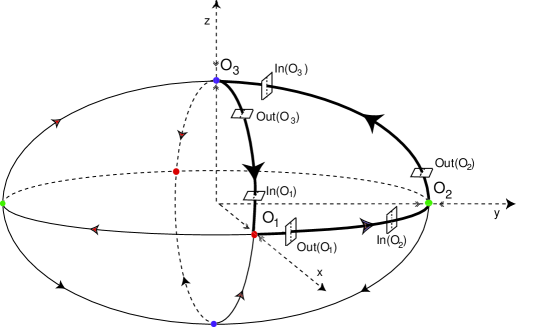
Figure 4. Cross sections near the hyperbolic equilibria of the May and Leonard cycle $\Gamma_{1}$ (restriction of $\Gamma$ to the first octant).

The set ${\text{In}}(O_{i})$ contains initial conditions where the points go inside $V_{i}$ in positive time; the set ${\text{Out}}(O_{i})$ contains initial conditions that leave $V_{i}$ in positive time.

For $\gamma\in[0,\gamma_{i}]$, let $q_{0}=(x_{s}(0),\,x_{r}(0),\,x_{u}(0),\,\theta(0))\in{\text{In}}(O_{i})\times{\mathbb{S}}^{1}$ and let

$$\left\{\begin{array}[]{l}q(t,q_{0};\gamma)=(x_{s}(t,q_{0};\gamma),\quad x_{r}(t,q_{0};\gamma),\quad x_{u}(t,q_{0};\gamma),\quad\theta(t,q_{0};\gamma))\\ \\ q(0,q_{0};\gamma)=q_{0}.\end{array}\right.$$

Integrating (5.1), we get:

$$\left\{\begin{array}[]{l}x_{s}(t,q_{0};\gamma)=x_{s}(0)\,\exp(t\,(-c+w_{s}(t,q_{0};\gamma))\\ \\ x_{r}(t,q_{0};\gamma)=x_{r}(0)\,\exp(t\,(-1+w_{r}(t,q_{0};\gamma))\\ \\ x_{u}(t,q_{0};\gamma)=x_{u}(0)\,\exp(t\,(e+w_{u}(t,q_{0};\gamma))\\ \\ \theta(t,q_{0};\gamma)=\theta(0)+2\omega\,t\end{array}\right.$$ (5.2)

where

$$w_{j}(t,q_{0};\gamma)=\frac{1}{t}\int_{0}^{t}\gamma\,g_{j}(q(s,q_{0};\gamma);\gamma)\,ds.$$

Proposition 5.5 of [28] asserts that there exists $K_{2}>0$ such that the following statement holds: for any $T^{\star}>1$ such that all solutions of (5.1) that start in ${\text{In}}(O_{i})\times{\mathbb{S}}^{1}$ remain in $V_{i}\times{\mathbb{S}}^{1}$ up to time $T^{\star}$, we have:

$$\|w_{j}\|_{C^{3}}<\gamma\,K_{2}.$$

As well as the values of the coordinates, the non-autonomous nature of the dynamics require us to keep track of the elapsed time spent on each part of the solution between the cross sections ${\text{In}}(O_{i})$ and ${\text{Out}}(O_{i})$.

Let $q_{0}\in{\text{In}}(O_{i})\times{\mathbb{S}}^{1}$, $\gamma\in\,]\,0,\gamma_{i}\,[$ and let $T(q_{0};\gamma)$ be the time at which the solutions of (5.2) starting from $q_{0}$ reaches ${\text{Out}}(O_{i})$. The time of flight is defined by:

$$T(q_{0};\gamma)=\frac{1}{e+w_{u}(T(q_{0},\gamma),q_{0};\gamma)}\ln\left(\frac{1}{\gamma\,x_{u}(0)}\right).$$

Proposition 5.7 and Lemma 7.4 of [28] provide a precise $C^{3}$–control of $T$. Check also the last paragraph of [28, §7].

5.2.2. Global map

The derivation of the Poincaré map also involves the calculation of the global maps between cross-sections. According to [26], for $i=1,2,3$, the global maps

$${\text{Out}}(O_{i})\rightarrow{\text{In}}\left(O_{(i+1)\text{mod}\,3}\right)$$

are invertible linear maps. The time that elapses during the transition between these cross-sections will be denoted by $\Delta_{i}\geq 0$. See formulas (16), (19), (21) and (24) of [2].

5.2.3. The return map

We are interested in an expression for the first return map from ${\text{In}}(O_{3})\backslash W^{s}(O_{3})$ to itself. From now on, as suggested in Figure 5, we consider just two coordinates of ${\text{In}}(O_{3})$:

$$(x,z)\mapsto(x_{u},1,x_{r})\in{\text{In}}(O_{3}).$$

In the region of the space of parameters defined by (C1a), the degree of the variables in the first phase coordinate ($x$) is smaller than that of the second ($z$).

The authors of [26] proved that, for $\gamma\geq 0$, there is $\tilde{\varepsilon}>0$ (small) such that a solution of (1.1) that starts in $\Sigma={\text{In}}(O_{3})\backslash W^{s}(O_{3})$ at time $s$, returns to $\Sigma$, with the dynamics dominated by the coordinate $x$, defining a map on the cylinder

$$(x,s)\in\mathcal{D}:=\{x/\tilde{\varepsilon}\in\,\,]\,0,1]\quad\text{and}\quad s\in{\mathbb{R}}\pmod{\pi/\omega}\},$$

that may be approximated by:

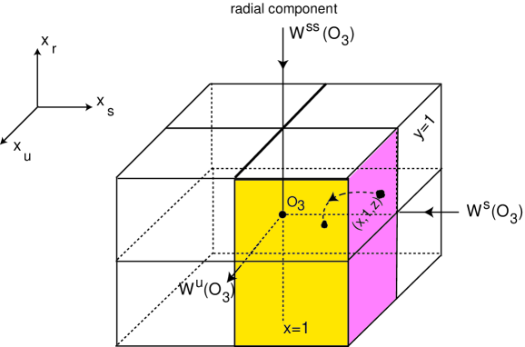
Figure 5. Scheme of the cross sections ${{\text{In}}(O_{3})}$ [pink] and ${\text{Out}}(O_{3})$ [yellow] in the neighbourhood $V_{3}$ of $O_{3}$. The set $W^{ss}(O_{3})$ corresponds to the local strong stable manifold of $O_{3}$; it corresponds to the radial direction.

$$\mathcal{F}^{1}_{\gamma}(x,s) = \mu x^{\delta}+\gamma\left[\mu_{1}+\mu_{2}L_{1}(x,s)-\mu_{4}G_{1}(x,s)-\mu_{5}G_{2}(x,s)\right]+O(\gamma^{2})$$

$$\mathcal{F}^{2}_{\gamma}(x,s) = s+\mu_{3}-\xi\log(x)-\frac{\gamma\,\xi}{x}L_{2}(x,s)+O(\gamma^{2})\quad\pmod{\pi/\omega}$$

where $\mu_{1}$, $\mu_{2}$, $\mu_{3}$, $\mu_{4}$ and $\mu_{5}$ are real constants (in general they are not computable analytically) that depend on the global maps, and

$$L_{1}(x,s) = \exp({-c\,(T_{3}(0)-T_{2}(0)-\Delta_{2})})\int_{T_{2}(0)+\Delta_{3}}^{T_{3}(0)}\exp(c(\tau-T_{2}(0)-\Delta_{2})g(2\omega\tau)\,d\tau$$

$$L_{2}(x,s) = \int_{t}^{T_{1}(0)}\exp(-e(\tau-t))g(2\omega\tau)\,d\tau$$

$$G_{1}(x,s) = \frac{1}{\exp(c\pi/\omega)-1}\int_{0}^{\pi/\omega}\exp(c\tau)g(2\omega(T_{3}(\gamma)+\tau))\,d\tau$$

$$G_{2}(x,s) = \frac{1}{\exp(-e\pi/\omega)-1}\int_{0}^{\pi/\omega}\exp(-e\tau)g(2\omega(T_{3}(\gamma)+\Delta_{3}+\tau))\,d\tau$$

$$T_{1}(0) = s-\frac{1}{e}\log(x)$$

$$T_{2}(0) = s+\Delta_{1}-\frac{e+c}{e^{2}}\log(x)$$

$$T_{3}(\gamma) = s+\Delta_{1}+\Delta_{2}-\frac{e^{2}+ce+c^{2}}{e^{3}}\log(x)$$

$$-\gamma\left[\frac{e^{2}+ce+c^{2}}{e^{3}x}\times\int_{s}^{T_{1}(0)}\exp(-e(\tau-s)g(2\omega\tau)\,d\tau)\right]+O(\gamma^{2}).$$

The expression of the first return map given in Theorem 3.1 may be now derived, assuming $g(2\omega t)=\sin^{2}(\omega\,t)$. Refining the expression of $L_{2}$, we get:

$$L_{2}(x,s) = \int_{s}^{T_{1}(0)}\exp(-e(\tau-s))\sin^{2}(\omega\tau)\,d\tau$$

$$= \frac{e^{2}+2\omega^{2}-e^{2}\cos^{2}(\omega\,s)+2\omega e\sin(\omega s)\cos(\omega s)}{e\,(e^{2}+4\omega^{2})}$$

$$= \frac{e^{2}\cos^{2}(\omega s)+2\omega^{2}}{e\,(e^{2}+4\omega^{2})}+\frac{e^{2}(1-2\cos^{2}(\omega s))}{e\,(e^{2}+4\omega^{2})}+\frac{\omega\,e\sin(2\omega s)}{e\,(e^{2}+4\omega^{2})}$$

$$= \frac{1}{e}\left(\eta_{\omega}(x,s)-a_{2}\cos(2\omega s)+b_{2}\cos(2\omega s)\right)$$

where

$$\eta_{\omega}(x,s):=\frac{e^{2}\cos^{2}(\omega s)+2\omega^{2}}{(e^{2}+4\omega^{2})}.$$

The map $\eta_{\omega}$ does not depend on $x$ and

$$\lim_{\omega\rightarrow 0}\eta_{\omega}(x,s)=1\qquad\text{and}\qquad\lim_{\omega\rightarrow+\infty}\eta_{\omega}(x,s)=\frac{1}{2},$$

making a complete agreement between our analysis and that of [26].

5.3. Digestive remarks

For $\tilde{\gamma}=\min\{\gamma_{1},\gamma_{2},\gamma_{3}\}$, we offer the following remarks concerning the expression of $\mathcal{F}_{\gamma}$, $\gamma\in[0,\tilde{\gamma}]$.

Remark 5.3.

When $\gamma=0$, for $\mu=1$ and $x>0$, we may write:

$$\mathcal{F}_{0}(x,s)=(x^{\delta},\,\,s+\omega\mu_{3}/\pi-\omega\xi\log(x)/\pi\pmod{1}).$$

This means that the $x$-component is contracting ($\delta>1$) and thus the dynamics of $\mathcal{F}_{0}$ is governed by the $s$-component. This is consistent to the fact that the network $\Gamma$ is asymptotically stable. In particular, $\displaystyle\lim_{x\rightarrow 0}\mathcal{F}_{0}(x,s)=(0,+\infty).$ Note that the computations of Section 6 do not hold for $\gamma=0$ due to the change of coordinates (6.1).

Remark 5.4.

The authors of [26] have provided an approximation of $\mathcal{F}_{\gamma}$ in the $C^{1}$–norm since they used a linearisation form. Assuming that $c$ and $e$ satisfy the Diophantine nonresonance Condition (C2), using the arguments of [28] revisited in §5.2.1, the approximation $\mathcal{F}_{\gamma}$ holds in the $C^{3}$–topology.

5.4. Proof of Proposition 3.2

Using (3.2), Hypothesis (C2) and the identity

$$\forall y\in{\mathbb{R}},\quad\forall x\in{\mathbb{R}}\backslash\{0\},\quad\exists a\in[0,2\pi[:\qquad x\cos a+y\sin a=\sqrt{x^{2}+y^{2}\,}\,\cos\left(\arctan\left(\frac{y}{x}\right)+a\right),$$ (5.3)

the expression of $\mathcal{F}_{\gamma}$ may be rewritten as (see Lemma 5.1):

$$\left\{\begin{array}[]{l}\mathcal{F}^{1}_{\gamma}(x,s)=x^{\delta}+\gamma\mu_{1}(1-\sqrt{a_{1}}\cos(2\omega s))\\ \\ \mathcal{F}^{2}_{\gamma}(x,s)=\displaystyle s+\mu_{3}-\xi\log(x)-\displaystyle\frac{\xi\gamma}{e}\frac{(1-\sqrt{a_{2}}\cos(2\omega s))}{x}\pmod{\pi/\omega}.\\ \end{array}\right.$$ (5.4)

Taking into account that $\displaystyle\lim_{\omega\rightarrow 0}a_{1}(\omega)=\lim_{\omega\rightarrow 0}a_{2}(\omega)$ and making the change of coordinates

$$s_{\,\text{new}}\mapsto\frac{\omega}{\pi}\,\,s_{\,\text{old}},$$

we get:

$$\left\{\begin{array}[]{l}\mathcal{F}^{1}_{\gamma}(x,s)=x^{\delta}+\gamma\mu_{1}(1-\sqrt{a_{1}}\cos(2\pi s))\\ \\ \mathcal{F}^{2}_{\gamma}(x,s)=\displaystyle s+\frac{\mu_{3}\omega}{\pi}-\frac{\xi\omega}{\pi}\log(x^{\delta}+\gamma\mu_{1}(1-\sqrt{a_{1}}\cos(2\pi s)))+O(\gamma^{2})\,\pmod{1}\\ \end{array}\right.$$ (5.5)

The $\gamma^{2}$–terms that appear in $\mathcal{F}^{2}_{\gamma}(x,s)$ arise in the Taylor $\gamma$–expansion of

$$\log(x^{\delta}+\gamma\mu_{1}(1-\sqrt{a_{1}}\cos(2\pi s)))$$

and hence they are collected in the expression $\mathcal{O}(\gamma^{2})$. Afraimovich et al [2] refer to equations (5.5) as a dissipative separatrix map since it corresponds to the return maps near separatrices in perturbed Hamiltonian systems when $\delta=1$. The resonant case $\delta=1$ has also been studied in [22].

5.5. Proof of Proposition 3.5

Taking into account that

$$\lim_{\omega\rightarrow+\infty}\eta_{\omega}(x,s)=\frac{1}{2},\qquad\lim_{\omega\rightarrow+\infty}\arctan\left(\frac{b_{2}(\omega)}{a_{2}(\omega)}\right)=\frac{\pi}{2},$$

using equality (5.3), we get:

$$\mathcal{F}^{2}_{\gamma}(x,s) = s+\mu_{3}-\xi\log(x)-\frac{\xi\gamma}{\,e}\frac{(1/2-\sqrt{a_{2}}\cos(2\omega s-\pi/2))}{x}+O(\gamma)\pmod{\omega/\pi}.$$

With $\mu=1$, since $\displaystyle\lim_{\omega\rightarrow+\infty}a_{1}(\omega)=0$, we may write:

$$\left\{\begin{array}[]{l}\mathcal{F}^{1}_{\gamma}(x,s)=x^{\delta}+\gamma\mu_{1}\\ \\ \mathcal{F}^{2}_{\gamma}(x,s)=\displaystyle s+\frac{\omega\mu_{3}}{\pi}-\frac{\xi\omega}{\pi}\log(x^{\delta}+\gamma\mu_{1})-\frac{\gamma\xi\omega}{2\,e\,\pi\,(x^{\delta}+\gamma\mu_{1})}+\frac{\gamma\,\omega\,\xi\sqrt{a_{2}}}{\,\pi\,e\,(x^{\delta}+\gamma\mu_{1})}\sin(2\pi s)\pmod{1}.\\ \end{array}\right.$$ (5.6)

Bear in mind that

$$\lim_{\omega\rightarrow+\infty}\left[\sqrt{a_{2}(\omega)}\big{/}\frac{e}{2\omega}\right]=1\quad\text{and}\quad\displaystyle\lim_{\omega\rightarrow+\infty}\left[\sqrt{a_{2}(\omega)}-\frac{e}{2\omega}\right]=0,$$

up to $\mathcal{O}(x^{\delta})$–terms, we obtain the one-dimensional reduction given in Proposition 3.5 by:

$$\left\{\begin{array}[]{l}\mathcal{F}^{1}_{\gamma}(x,s)=\gamma\,\mu_{1}\\ \\ \mathcal{F}^{2}_{\gamma}(x,s)=\displaystyle s+\frac{\omega\mu_{3}}{\pi}-\frac{\xi\omega}{\pi}\log(\gamma\,\mu_{1})-\frac{\xi\omega}{2\,e\,\mu_{1}\,\pi}+\frac{\xi}{2\,\pi\,\mu_{1}}\sin(2\pi s)\pmod{1}.\\ \end{array}\right.$$ (5.7)

6. Proof of Theorem A

The purpose of this section is to prove the main result of this manuscript. Our starting point is the expression (3.3) with $\mu_{1}=1$ and $\omega\approx 0$ fixed. Recall that $\tilde{\gamma}=\min\{\gamma_{1},\gamma_{2},\gamma_{3}\}$.

6.1. Change of coordinates

For $\gamma\in\,\,]0,\tilde{\gamma}[$ fixed and $(x,s)\in\tilde{\mathcal{D}}$, let us make the following change of coordinates:

$$x_{\,\text{new}}\mapsto\gamma^{-\frac{1}{\delta}}x_{\text{old}}.$$ (6.1)

Observe that

$$\mathcal{F}^{1}_{\gamma}(x_{\,\text{new}},s)=\gamma\left(\left(\frac{x_{\,\text{old}}}{\gamma^{\frac{1}{\delta}}}\right)^{\delta}+\left[1-\sqrt{a_{1}}\cos(2\pi s)\right]\right)=\gamma^{p}\left({x_{\,\text{new}}}^{\delta}+\left[1-\sqrt{a_{1}}\cos(2\pi{s})\right]\right),$$

for some $p>0$. Setting $(x_{\,\text{new}},s)\equiv(x,s)$, we get:

$$\mathcal{F}^{1}_{\gamma}(x,s) = \gamma^{p}\left({x}^{\delta}+\left[1-\sqrt{a_{1}}\cos(2\pi{s})\right]\right)$$

$$\mathcal{F}^{2}_{\gamma}(x,s) = {s}+\frac{\mu_{3}\,\omega}{\pi}-\frac{\xi\,\omega\,p}{\pi}\ln(\gamma)-\frac{\xi\,\omega}{\pi}\log\left({x}^{\delta}+\left[1-\sqrt{a_{1}}\cos(2\pi{s})\right]\right).$$

We now view the family of maps $\mathcal{F}_{\gamma}=(\mathcal{F}^{1}_{\gamma},\mathcal{F}^{2}_{\gamma})$ as a two-parameter family of embeddings satisfying the Hypotheses (H1)–(H7) of Subsection 4.2.

6.2. Reduction to a singular limit

For $\gamma\in\,\,]\,0,\tilde{\gamma}\,[$, we compute the singular limit associated to $\mathcal{F}_{\gamma}$ written in the coordinates $(x,s)$ defined in Subsection 6.1. Let $k:{\mathbb{R}}^{+}\rightarrow{\mathbb{R}}$ be the invertible map defined by

$$k(x)=-K_{\omega}\,\xi\ln(x),\qquad\text{where}\qquad K_{\omega}=\frac{\omega\,p}{\pi}>0.$$

As suggested in Figure 6, define the decreasing sequence $(\gamma_{n})_{n}$ such that, for all $n\in{\mathbb{N}}$:

1. $\gamma_{n}\in\,]0,\tilde{\gamma}[$ and
   

2. $k(\gamma_{n})\equiv 0\mod 1$.

Since $k$ is an invertible map, for $a\in{\mathbb{S}}^{1}\equiv[0,1[$ fixed and $n\geq n_{0}\in{\mathbb{N}}$, let

$$\gamma_{(a,n)}=k^{-1}\left(k(\gamma_{n})+a\right)\,\,\in\,\,]\,0,\tilde{\gamma}\,[.$$ (6.2)

It is immediate to check that:

$$k(\gamma_{(a,n)})=-K_{\omega}\,\xi\ln(\gamma_{n})+a=a\mod 1.$$ (6.3)

The following proposition establishes the $C^{3}$–convergence to a singular limit, as $n\rightarrow+\infty$ (defined in the appropriate set of maps from $\tilde{\mathcal{D}}$ to ${\mathbb{R}}$).

Lemma 6.1.

In the $C^{3}$–Whitney topology, the following equality holds:

$$\lim_{n\in{\mathbb{N}}}\|\mathcal{F}_{\gamma_{(n,a)}}-(\textbf{0},h_{a})\|=0$$

where 0 represents the null map and

$$h_{a}(x,s)=s+a-\frac{\xi\,\omega}{\pi}\log\left[(1-\sqrt{a_{1}}\cos(2\pi{s}))\right].$$ (6.4)

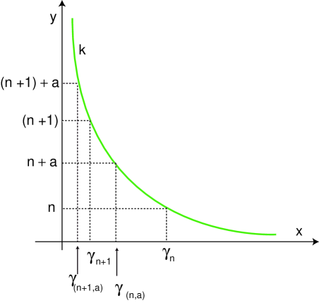
Figure 6. Graph of the map $k(x)=-K_{\omega}\,\xi\ln(x)$ for $\displaystyle K_{\omega}=\frac{\omega\,p}{\pi}$, and illustration of the sequences $(\gamma_{n})_{n}$ and $(\gamma_{(n,a)})_{n}$ for a fixed $a\in[0,1[$.

Proof.

Using (6.3), note that

$$\mathcal{F}^{1}_{\gamma_{(n,a)}}(x,{s}) = \gamma_{(n,a)}^{p}\left({x}^{\delta}+\left[1-\sqrt{a_{1}}\cos(2\pi{s})\right]\right)$$

$$\mathcal{F}^{2}_{\gamma_{(n,a)}}(x,s) = {s}+\frac{\mu_{3}\,\omega}{\pi}-K_{\omega}\,\xi\ln(\gamma_{(n,a)})-\frac{\xi\,\omega}{\pi}\log\left[{x}^{\delta}+\left[1-\sqrt{a_{1}}\cos(2\pi{s})\right]\right]$$

$$= {s}+\frac{\mu_{3}\,\omega}{\pi}+a-\frac{\xi\,\omega}{\pi}\log\left[{x}^{\delta}+\left[1-\sqrt{a_{1}}\cos(2\pi{s})\right]\right].$$

Therefore, since $\displaystyle\lim_{n\in{\mathbb{N}}}{\gamma_{(n,a)}}=0$ we may write:

$$\lim_{n\in{\mathbb{N}}}\mathcal{F}^{1}_{\gamma_{(n,a)}}(x,{s}) = 0$$

$$\lim_{n\in{\mathbb{N}}}\mathcal{F}^{2}_{\gamma_{(n,a)}}(x,{s}) = s+\frac{\mu_{3}\,\omega}{\pi}+a-\frac{\xi\,\omega}{\pi}\ln\left(1-\sqrt{a_{1}}\cos(2\pi{s}\right))\pmod{1}$$

and we get the result.

∎

Remark 6.2.

The map $h_{a}(x,s)$ just depends on $s$:

$$h_{a}(x,s)\equiv\mathcal{F}^{2}_{\gamma_{(n,a)}}(0,s)=s+\frac{\mu_{3}\,\omega}{\pi}+a-\frac{\xi\,\omega}{\pi}\ln\left(1-\sqrt{a_{1}}\cos(2\pi{s}\right)),$$

this is why in §6.3, we identify $h_{a}(x,s)$ and $h_{a}(s)$. The map $h_{a}(s)$ is a Morse function and has finitely many nondegenerate critical points (note that $\sqrt{a_{1}}<1$).

6.3. Verification of the hypotheses of the theory of rank-one maps.

From now on, our focus will be the sequence of two-dimensional maps

$$F_{(a,b)}=\mathcal{F}_{(a,\gamma(n,a))}\qquad\text{with}\qquad n\in\mathbb{N}\qquad\text{and}\qquad a\in[\,0,1[\text{ fixed}.$$ (6.5)

Since our starting point is an attracting heteroclinic network (for $\gamma=0$), the absorbing sets defined in Subsection 2.4 of [30] follow from the existence of the attracting annular region ensured by next result:

Lemma 6.3 ([2, 26], adapted).

There exists $\gamma^{\star}>0$ small such that for all $\gamma\in\,]\,0,\gamma^{\star}\,]$, the region

$$\mathcal{B}=\left\{(x,s)\in\tilde{\mathcal{D}}:\qquad 0<x^{\star}-2\gamma\sqrt{a_{1}}\leq x\leq x^{\star}+2\gamma\sqrt{a_{1}},\qquad s\in[0,1[\,\right\}$$

is forward-invariant set under $\mathcal{F}_{\gamma}$–interation, corresponding to the shaded region of Figure 8.

Now, we show that the family of maps (6.5) satisfies Hypotheses (H1)–(H7) stated in Subsection 4.2.

(H1):

The first two items are immediate. We establish the distortion bound (H1)(3) by studying $D\mathcal{F}_{(a,\gamma(n,a))}$. Direct computation implies that for every $\gamma\in(0,\tilde{\gamma})$ and $(x,s)\in\tilde{\mathcal{D}}$, one gets:

$$D\mathcal{F}_{(a,\gamma(n,a))}({x},{s})=\left(\begin{array}[]{cc}\displaystyle\frac{\partial\mathcal{F}_{(a,\gamma(n,a))}^{1}(x,s)}{\partial{x}}&\displaystyle\frac{\partial\mathcal{F}_{(a,\gamma(n,a))}^{1}(x,s)}{\partial{s}}\\ \\ \displaystyle\frac{\partial\mathcal{F}_{(a,\gamma(n,a))}^{2}(x,s)}{\partial{x}}\displaystyle&\displaystyle\frac{\partial\mathcal{F}_{(a,\gamma(n,a))}^{2}(x,s)}{\partial{s}}\end{array}\right)$$

where

$$\frac{\partial\mathcal{F}_{(a,\gamma(n,a))}^{1}({x},{s})}{\partial{x}} = \gamma_{(n,a)}^{p}\,\delta{x}^{\delta-1}$$

$$\frac{\partial\mathcal{F}_{(a,\gamma(n,a))}^{1}({x},{s})}{\partial{s}} = 2\,\pi\,\gamma_{(n,a)}^{p}\,\sqrt{a_{1}}\sin(2\pi{s})$$

$$\frac{\partial\mathcal{F}_{(a,\gamma(n,a))}^{2}({x},{s})}{\partial{x}} = -\xi\frac{\omega}{\pi}\left(\frac{\delta{x}^{\delta-1}}{{x}^{\delta}+(1-\sqrt{a_{1}}\cos(2\pi{s}))}\right)$$

$$\frac{\partial\mathcal{F}_{(a,\gamma(n,a))}^{2}({x},{s})}{\partial{s}} = 1-\xi\frac{\omega}{\pi}\left(\frac{2\pi\,\sqrt{a_{1}}\sin(2\pi{s})}{{x}^{\delta}+\gamma(1-\sqrt{a_{1}}\cos(2\pi{s}))}\right)$$

and therefore

$$|\det D\mathcal{F}_{(a,\gamma(n,a))}(x,{s})|=\gamma_{(n,a)}^{p}\delta x^{\delta-1}.$$

Since $x>0$ (Lemma 6.3), we conclude that there exists $\gamma^{\star}>0$ small enough such that:

$$\forall\gamma\in\,]\,0,\gamma^{\star}\,[,\qquad\det D\mathcal{F}_{\gamma}(x,{s})|\in\,\,]\,k_{1}^{-1},k_{1}\,[,$$

for some $k_{1}>1$. This implies that Hypothesis (H1)(3) is satisfied.

(H2) and (H3):

It follows from Lemma 6.1 where $b=\gamma_{(n,a)}$.

(H4) and (H5):

These hypotheses are connected with the family of circle maps

$$h_{a}:{\mathbb{S}}^{1}\rightarrow{\mathbb{S}}^{1}$$

defined in Remark 6.2, noting that $\mathcal{F}^{2}_{\gamma_{(n,a)}}(0,s)\equiv h_{a}(s)$. Taking into account Proposition 2.1 of [31], there exists $\xi^{\star}\in{\mathbb{R}}^{+}$ such that if $\xi>\xi^{\star}$, the family

$$h_{a}(s)=s+\frac{\mu_{3}\,\omega}{\pi}+a-\frac{\xi\,\omega}{\pi}\log(1-\sqrt{a_{1}}\cos(2\pi s))\qquad a\in[\,0,1\,[$$

satisfies Properties (H4) and (H5).

(H6):

The computation follows from direct computation using the expression of $\mathcal{F}_{\gamma}(x,s)$. Indeed, for each $s\in C_{a^{\star}}$ (set of critical points of $h_{a^{\star}}$), we have

$$\frac{d}{dx}\mathcal{F}_{(a^{\star},0)}(x,s)|_{x=0}=1.$$

(H7):

It follows from Proposition 2.1 of [31] if $\xi$ is large enough ($\Rightarrow$ the “big lobe” of [27] is large enough).

Since the family $\mathcal{F}_{(a,\gamma(n,a))}$ satisfies (H1)–(H7) then, for $\gamma^{+}=\min\{\tilde{\gamma},\gamma^{\star}\}>0$, if $\xi>\xi^{\star}$, there exists a subset $\Delta\in[0,\gamma^{+}]$ with positive Lebesgue measure such that for $\gamma\in\Delta$, the map $\mathcal{F}_{\gamma}$ admits a strange attractor

$$\Omega\subset\bigcap_{m=0}^{+\infty}\mathcal{F}_{\gamma}^{m}(\tilde{\mathcal{D}})$$

supporting a unique ergodic SRB measure $\nu$. The orbit of Lebesgue almost all points in ${\Omega}$ has positive Lyapunov exponent and is asymptotically distributed according to $\nu$. The abundance of strange attractors follows from §3 of [28].

Remark 6.4.

The strange attractor $\Omega$ is non-uniformly hyperbolic, non-structurally stable and is the limit of an increasing sequence of uniformly hyperbolic invariant sets.

The proof of [29] goes further. The pair $(\mathcal{F}_{\gamma},\nu)$ has exponential decay of correlations for Holder continuous observables: given an Holder exponent $\eta$, there exists $\tau=\tau(\eta)<1$ such that for all Holder maps $\varphi$, $\psi:\Omega\rightarrow{\mathbb{R}}$ with Holder exponent $\eta$, there exists $K(\varphi,\psi)\geq 0$ such that for all $m\in{\mathbb{N}}$, we have:

$$\left|\int(\varphi\circ\mathcal{F}_{\gamma}^{m})\psi\,d\nu-\int\varphi d\nu\int\psi d\nu\right|\leq K(\varphi,\psi)\tau^{m}.$$

7. From the attracting torus to strange attractors:
a geometrical interpretation

In this section, we give a geometrical interpretation of the mechanisms behind the creation of rank-one strange attractors. We also compare our results with previous works in the literature.

With respect to the original equation (1.1), borrowing the ideas of [2], for $\omega>0$ fixed, we may draw two smooth curves, the graphs of $t_{1}$ and $t_{2}$ shown in Figure 7, such that:

1. $\displaystyle t_{1}(\xi)=\frac{\exp(C/\xi\omega)-1}{\exp(C/\xi\omega)-1/C}$, $C>2$, and $\displaystyle t_{2}(\xi)=1/\sqrt{1+(\xi\omega)^{2}}$;

2. the region above the graph of $t_{1}$ corresponds to vector fields whose flows exhibit suspended rotational horseshoes [21] (compare with Theorem 3.4 in Section 3);

3. the region below the graph of $t_{2}$ corresponds to flows having an invariant and attracting torus with zero topological entropy.

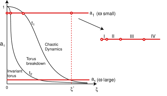
Figure 7. Graphs of $t_{1}$ and $t_{2}$ and the relative position of $a_{1}$ for $\omega$ small and large (cf. Lemma 5.1). I - attracting curve; II - torus-breakdown bifurcations associated to an Arnold tongue; III - Rotational horseshoes; IV - rank-one strange attractors.

From now on, we focus on Cases 3 and 4 of Table 2 ($\omega\approx 0$). For $\delta\gtrsim 1$, if $\xi$ is small enough then the initial deformation of the singular limit is suppressed by the “contracting force” and the maximal attracting set is a non-contractible closed curve satisfying Afraimovich’s Annulus Principle [2]. This is consistent with the results stated in [25] about the existence of an attracting curve for the map $\mathcal{F}_{\gamma}$. The parameters considered in [9] do not allow to see observable chaos since the parameter $\displaystyle\xi=\frac{1+\delta+\delta^{2}}{e}$ for $\delta\gtrsim 1$, cannot be large enough.

If $\delta\gg 1$ (region I of [25]), then $\xi$ may be either small or large. If $\xi$ is small, the flow of (1.1) has again an attracting normally hyperbolic torus. If $\xi$ is large, then the initial deformation brought by the perturbing term is exaggerated. The attracting region $\mathcal{B}$ (Lemma 6.3) starts to disintegrate into a finite collection of periodic saddles and sinks, a phenomenon occurring within an Arnold tongue [4]. These bifurcations correspond to what the authors of [30] call transient chaos associated to the Torus-breakdown bifurcations [1, 4, 24]. The curves $\mathcal{H}_{n}$ of Figure 14 of [26] indicate the location of homoclinic bifurcations involving the $n$-period orbit within the corresponding Arnold tongue. As discussed in Section 5 of [8], a homoclinic bifurcation occurs when the set of preimages of an unstable period-$n$ orbit of $h_{a}(s)$ contains a critical point (minimum or maximum), giving rise to chaotic dynamics, not necessarily observable.

As $\xi$ gets larger ($\xi>\xi^{\star}$), the initial deformation introduced by the perturbing term is exaggerated further, getting us the emergence of rank-one attractors (Theorem A), obtained by stretch and fold. These two mechanisms are due to the attracting features of $\Gamma$ combined with the presence of non-degenerated turns of the circle map $h_{a}$. Points of the singular limit ensured by (H2), at different distances from $x=0$, rotate at different speeds. As $\gamma$ varies, the two critical values of $h_{a}$ move at rates $1/\gamma$ in opposite directions. See an illustration of this mechanism in Figure 8.

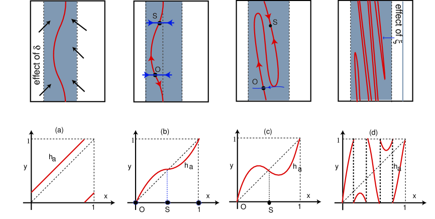
Figure 8. Illustration of the emergence of rank-one attractors for $\mathcal{F}_{\gamma}$ from the dynamics of $h_{a}(s)\pmod{1}$ when $\xi$ varies. (a) $\xi=\xi_{0}\gtrsim 0$ – attracting torus. (b) $\xi=\xi_{1}$ – attracting torus inside resonance tongue with a saddle and a sink. (c) $\xi=\xi_{2}$ – torus-breakdown. (d) $\xi=\xi^{\star}$ – mixing properties (isomorphic to a Bernoulli shift).

For $\omega\approx 0$ and $\delta\gg 1$, the dynamics of the first return map is chaotic and no longer reducible to a one dimensional map. Nevertheless, according to [30], certain “good” properties of the singular cycle may be passed back to the two-dimensional system (see Remark 6.2). Forgetting temporarily its connection to equation (6.4), we might think of $h_{a}$ as an abstract circle map.

• If $h_{a}$ is a diffeomorphism, the classical theory by Denjoy may be applied. We point out a resemblance between “our” $h_{a}$ and the family of circle maps first studied in [4]. Because of strong normal contraction, invariant curves are shown to exist independent of rotation number.

• If $h_{a}$ is not invertible, two types of dynamical behaviours are known to be prevalent. There is some evidence that these are only two observable pure dynamics types: maps with sinks or maps with absolutely continuous invariant measures. Wang and Young’s theory [30] provides the bridge from the non-invertible circle maps theory to dissipative systems of the form (3.3).

For $\gamma>0$ fixed, the evolution of $h_{a}$ as $\xi$ varies, is suggested in Figure 8. In (a) and (b), we see the existence of an invariant curve (giving rise to an attracting torus). In case (b) we may see the existence of two fixed points, suggesting that the chosen parameters are within a resonant wedge [4]. In (c), the map $h_{a}$ is not a diffeomorphism meaning that the invariant torus is broken; it corresponds to the point when the unstable manifold of the saddle $O$ (in the Arnold tongue [4]) turns around. In case (d), the Property (H7) holds, meaning that the unstable manifold of the saddle $O$ crosses each leaf of the stable foliation of other saddles of the torus’s ghost. Figure 4 of [30] is particularly suggestive to understand this phenomenon. As a conclusion, we may give a geometrical interpretation of the parameters in our context (see Figure 8):

$$\delta>1 \mapsto (\tilde{\mathcal{D}}$$ forces the existence of an invariant attracting region );

$$\xi\gg 0 \mapsto$$ forces the large number of turns of the singular limit

plays the same role as the twisting number of [24];

$$\omega>0 \mapsto \text{governs the amplitude of the non-autonomous perturbation of }\mathcal{F}_{\gamma}$$

(recall that $$a_{1} \omega$$ depends on );

$$\gamma>0 \mapsto$$ inverse of the dissipation.

8. Discussion

In this article, we have discussed the dynamics of a periodically-perturbed vector field in ${\mathbb{R}}^{3}$ whose unperturbed flow has a symmetric and clean attracting heteroclinic network. This work should be seen as the natural continuation of [26].

Based on the numerics of [9, 25], we distinguish four cases for the dynamics. In the case $\delta\gg 1$ and $\omega\approx 0$, we have refined the analysis of [26] and introduced a new parameter $\xi$. Taking into account the action of this new parameter, we have formulated a checkable hypothesis under which the map $\mathcal{F}_{\gamma}$, induced by the flow of the forced system, admits a strange attractor. It supports a unique ergodic SRB measure for a set $\Delta$ of forcing amplitudes with $Leb(\Delta)>0$. For all $\gamma\in\Delta$, the flow-induced map is rank-one in the sense of [30]; the chaos is observable and abundant. This result gives a rigorous answer to the problem raised in Section 8 of [20]. Before finishing the paper, we would like to stress the following two remarks:

1. Conditions (C1a) and (C1b) are the only hypotheses we really need to prove Theorem A. Condition (C2) simplifies the computations but it may be relaxed. All results are valid if $1-\sqrt{a_{1}}\cos(2\omega\Psi(0,s))$ (cf. (3.2)) is a positive Morse function with finitely many non-degenerate points, which is a generic requirement. See Proposition 2.1 of [31].

2. Although the non-autonomous perturbation term only acts on the $x$-coordinate in (1.1), the whole calculation can be carried out in the same way for any non-negative periodic forcing acting on all components. The use of other periodic forcing would lead qualitatively similar dynamical regimes. The only necessary requirement is that the external periodic forcing should be non-negative with small amplitude $\gamma$.

In summary, the forced May-Leonard system (1.1) or, equivalently, the forced Guckenheimer and Holmes system, may behave periodically, quasi-periodically or chaotically, depending on specific character of the forcing. Ergodic consequences of this article are in preparation.

References

- [1] V.S. Afraimovich, L.P. Shilnikov. On invariant two-dimensional tori, their breakdown and stochasticity in: Methods of the Qualitative Theory of Differential Equations, Gor’kov. Gos. University (1983), 3–26. Translated in: Amer. Math. Soc. Transl., (2), vol. 149 (1991) 201–212.
- [2] V.S. Afraimovich, S-B Hsu, H. E. Lin. Chaotic behavior of three competing species of May-Leonard model under small periodic perturbations. Int. J. Bif. Chaos, 11(2) (2001) 435–447.
- [3] V. Araújo, M. J. Pacífico. Three-dimensional flows. Springer Science & Business Media, (2010).
- [4] D. Aronson, M. Chory, G. Hall, R. McGehee. Bifurcations from an invariant circle for two-parameter families of maps of the plane: a computer-assisted study, Communications in Mathematical Physics, 83(3) (1982) 303–354.
- [5] P. Ashwin, P. Chossat. Attractors for robust heteroclinic cycles with continua of connections, Journal of Nonlinear Science, 8(2) (1998) 103–129.
- [6] P. Barrientos, J. A. Rodríguez, A. Ruiz-Herrera. Chaotic dynamics in the seasonally forced SIR epidemic model, Journal of mathematical biology 75:6-7 (2017): 1655–1668.
- [7] M. Benedicks, L. Carleson. The dynamics of the Hénon map, Annals of Mathematics 133(1) (1991) 73–169.
- [8] P. Boyland. Bifurcations of circle maps: Arnol’d tongues, bistability and rotation intervals. Communications in Mathematical Physics, 106 (3) (1986) 353–381.
- [9] J. Dawes, T.-L. Tsai. Frequency locking and complex dynamics near a periodically forced robust heteroclinic cycle, Phys. Rev. E, 74 (2006) 055201(R).
- [10] G. Gottwald, I Melbourne. A new test for chaos in deterministic systems, Proceedings of the Royal Society of London. Series A: Mathematical, Physical and Engineering Sciences 460.2042 (2004) 603–611.
- [11] J. Guckenheimer, P. Holmes. Nonlinear Oscillations, Dynamical Systems, and Bifurcations of Vector Fields, Applied Mathematical Sciences 42, Springer-Verlag, (1983).
- [12] J. Guckenheimer, P. Holmes. Structurally stable heteroclinic cycles, Math. Proc. Camb. Phil. Soc., 103 (1988) 189–192.
- [13] A.J. Homburg. Periodic attractors, strange attractors and hyperbolic dynamics near homoclinic orbits to saddle-focus equilibria. Nonlinearity 15 (2002) 1029–1050.
- [14] I.S. Labouriau, A.A.P. Rodrigues. Dense heteroclinic tangencies near a Bykov cycle, J. Diff. Eqs. 259(12) (2015) 5875–5902.
- [15] I.S. Labouriau, A.A.P. Rodrigues. Bifurcations from an attracting heteroclinic cycle under periodic forcing, J. Diff. Eqs., 269 (2020) 4137–4174.
- [16] R. Mackay, C. Tresser. Transition to topological chaos for circle maps, Physica D: Nonlinear Phenomena 19.2 (1986) 206–237.
- [17] R.M. May, W.J. Leonard. Nonlinear aspects of competition between three species, SIAM J. App. Math., 29.2 (1975) 243 –253.
- [18] M. Misiurewicz. Absolutely continuous measures for certain maps of an interval, Inst. Hautes Études Sci. Publ. Math. 53 (1981) 17–51.
- [19] L. Mora, M. Viana. Abundance of strange attractors, Acta Math. 171(1) (1993) 1–71.
- [20] A. Mohapatra, W. Ott. Homoclinic Loops, Heteroclinic Cycles, and Rank One Dynamics, SIAM Journal on Applied Dynamical Systems, 14(1) (2015) 107–131.
- [21] A. Passeggi, R. Potrie, M. Sambarino. Rotation intervals and entropy on attracting annular continua, Geometry & Topology 22(4) (2018) 2145–2186.
- [22] C. Postlethwaite, J. Dawes. Resonance bifurcations from robust homoclinic cycles, Nonlinearity 23(3) (2010) 621–642.
- [23] A.A.P. Rodrigues. Persistent switching near a heteroclinic model for the geodynamo problem, Chaos, Solitons & Fractals 47 (2013) 73–86.
- [24] A.A.P. Rodrigues. Unfolding a Bykov attractor: from an attracting torus to strange attractors, J. Dyn. Diff. Eqs. (2020), https://doi.org/10.1007/s10884-020-09858-z (to appear)
- [25] T.-L. Tsai, J. Dawes. Dynamics near a periodically forced robust heteroclinic cycle, J. Physics: Conference Series 286, (2001) 012057.
- [26] T.-L. Tsai, J. Dawes. Dynamic near a periodically-perturbed robust heteroclinic cycle, Physica D, 262 (2013) 14–34.
- [27] D. Turaev, L. P. Shilnikov. Bifurcations of quasiattractors torus-chaos, Mathematical mechanisms of turbulence (1986) 113–121.
- [28] Q. Wang, W. Ott. Dissipative homoclinic loops of two-dimensional maps and strange attractors with one direction of instability, Communications on Pure and Applied Mathematics 64–11 (2011) 1439–1496.
- [29] Q. Wang, L.-S. Young. Strange attractors with one direction of instability. Commun. Math. Phys. 218 (2001) 1–97.
- [30] Q. Wang, L.-S. Young. From Invariant Curves to Strange Attractors, Commun. Math. Phys. (2002) 225–275.
- [31] Q. Wang, L.-S. Young. Strange Attractors in Periodically-Kicked Limit Cycles and Hopf Bifurcations, Commun. Math. Phys. 240 (2003) 509–529.
- [32] Q. Wang, L..S. Young. Toward a theory of rank one attractors, Ann. of Math. (2) 167, (2008) 349–480.
- [33] L.-S. Young, M. Benedicks. Sinai-Bowen-Ruelle measures for certain Hénon maps. Inventiones mathematicae 112.3 (1993): 541–576.