Smaller World Models for Reinforcement Learning

Abstract

Sample efficiency remains a fundamental issue of reinforcement learning. Model-based algorithms try to make better use of data by simulating the environment with a model. We propose a new neural network architecture for world models based on a vector quantized-variational autoencoder (VQ-VAE) to encode observations and a convolutional LSTM to predict the next embedding indices. A model-free PPO agent is trained purely on simulated experience from the world model. We adopt the setup introduced by Kaiser et al. (2020), which only allows $100K$ interactions with the real environment. We apply our method on $36$ Atari environments and show that we reach comparable performance to their SimPLe algorithm, while our model is significantly smaller.

1 Introduction

Reinforcement learning is a generally applicable framework for finding actions in an environment that maximizes the sum of rewards. From a probabilistic perspective, the following probabilities lay the foundations of all reinforcement learning problems:

The dynamics ${p(r_{t},s_{t+1}\,|\,s_{t},a_{t})}$, i.e., the conditional joint probability of the next reward and state given the current state and action. This probability defines the environment and is usually unknown. In most real-world applications the underlying states $s_{t}$ are not observable, but instead the environment produces observations $x_{t}$, which might not contain all state information. In this case we can only observe ${p(r_{t},x_{t+1}\,|\,x_{t},a_{t})}$.

The policy ${p_{\theta}(a_{t}|x_{t})}$, i.e., the conditional probability of choosing an action given the current observation, where $\theta$ denotes the parameters of some model, indicating that this probability is not provided by the environment, but learned. Reinforcement learning methods provide means to optimize the policy in the sense that the actions that maximize the future sum of rewards have the highest probability.

Model-free algorithms try to optimize the policy ${p_{\theta}(a_{t}|x_{t})}$ based on real experience from the environment, without any knowledge of the underlying dynamics. They have shown great success in a wide range of environments, but usually require a large amount of training data, i.e., many interactions with the environment. This low sample efficiency makes them inappropriate for real-world applications in which data collection is expensive.

Model-based algorithms approximate the dynamics ${p_{\phi}(r_{t},x_{t+1}\,|\,x_{t},a_{t})\approx p(r_{t},x_{t+1}\,|\,x_{t},a_{t})}$, where $\phi$ denotes some learned parameters, thus building a model of the environment, which we will call world model to differentiate it from other models. The process of improving the policy using the world model is called planning, but there are two types: first, we can generate training data by sampling from ${p_{\phi}(r_{t},x_{t+1}\,|\,x_{t},a_{t})}$ and apply a model-free algorithm to this simulated experience. Second, we can try to look ahead into the future using the world model, starting from the current observation, in order to dynamically improve the action selection during runtime.

Contributions.

In this work we follow a model-based approach and consider the first type of planning. The ability to generate new experience without acting in the real environment does effectively increase the sample efficiency. Our main contributions and insights can be summarized as follows:

• VQ-VAE based world models require fewer parameters than previous approaches (see Table 2 and Table 3).

• Learning a latent space world model and training an agent on it is possible with only 100K interactions (see Table 4).

• A two-dimensional discrete latent representation combined with a dynamics network built from convolutional LSTMs (see Fig. 3) is sufficient for model-based training in Atari games.

2 Related Work

World Models (Ha & Schmidhuber, 2018).

Modeling environments with complex visual observations is a hard task, but luckily predicting observations on pixel level is not necessary. The authors introduce latent variables by encoding the high-dimensional observations $x_{t}$ into lower-dimensional, latent representations $z_{t}$. For this purpose they use a variational autoencoder (Kingma & Welling, 2014), which they call the “vision” component, that extracts information from the observation at the current time step. They use an LSTM combined with a mixture density network (Bishop, 1994) to predict the next latent variables stochastically. They call this component the “memory”, that can accumulate information over multiple time steps.

They also condition the policy on the latent variable, which enables them to stay in latent space, so that decoding back into pixels is not required (except for learning the representations). This makes simulation more efficient and can reduce the effect of accumulating errors. In Section 3.1 we describe in more detail how to integrate latent variables into the dynamics.

They successfully evaluate their architectures on two environments, but it involves some manual fine-tuning of the policy. They use an evolution strategy to optimize the policy, which is not suitable for bigger networks. They also use a non-iterative training procedure, i.e., they randomly collect real experience only once and then train the world model and the policy. This implies that the improved policies cannot be used to obtain new experience, and a random policy has to ensure sufficient exploration, which makes the approach inappropriate for more complex environments.

Simulated Policy Learning (Kaiser et al., 2020).

The authors introduce a new model-based algorithm (SimPLe) and successfully apply it to Atari games. They use an iterative training procedure, that alternates between collecting real experience, training the world model, and improving the policy using the world model.

Another novelty is that they restrict the algorithm to about $100K$ interactions with the real environment, which is considerably less than the usual $10M$ to $50M$ interactions.

They train the policy using the model-free PPO algorithm (Schulman et al., 2017) instead of an evolution strategy. They use a video prediction model similar to SV2P (Babaeizadeh et al., 2017) and incorporate the input action in the decoding process to predict the next frame. The latent variable is discretized into a bit vector, that is predicted autoregressively using an LSTM during inference time. The policy gets frames as input, which means that decoding the latent variables back into pixel-level is required.

They get very good results on a lot of Atari environments, considering the low number of interactions.

Dreamer (Hafner et al., 2020a) and DreamerV2 (Hafner et al., 2020b).

The architecture of DreamerV2 is closely related to ours. The authors train a world model with latent representations, such that the agent can operate directly on the latent variables. One of the main improvements of DreamerV2 over the model of Dreamer is the discretization of the latent space, as it uses categorical instead of Gaussian latent variables.

They show that their agent beats model-free algorithms in many Atari games after $50M$ interactions. This is a quite different goal from our work, where we attempt to learn as much as possible from only $100K$ interactions. Furthermore, we base our discrete latent world model on a VQ-VAE and thus discretize the latent variables using vector quantization.

3 Discrete Latent Space World Models

The goal of this work is to extend the idea of Ha & Schmidhuber (2018) by using more sophisticated neural network architectures and evaluating them on Atari environments with the model-free PPO algorithm instead of evolution strategies. In particular, we discretize the latent space, but have a fundamentally different architecture compared to DreamerV2 (Hafner et al., 2020b), since our latent space is two-dimensional. Moreover, we adopt the limitation to $100K$ interactions, the iterative training scheme and some other crucial ideas from Kaiser et al. (2020), which will be explained in later sections.

3.1 Latent Variables

Figure 1: Graphical model of the world model and the policy, which arises from inserting the latent variables and from our independence assumptions.

Similar to Ha & Schmidhuber (2018) we approximate the dynamics with the help of latent variables. The sum rule of probability allows us to introduce a latent variable $z_{t}$,

$$\begin{split}p(r_{t},x_{t+1}\,|\,x_{t},a_{t})\approx&\,\mathbb{E}_{z_{t}\sim p(z_{t}|x_{t})}\,\mathbb{E}_{z_{t+1}\sim p(z_{t+1}|z_{t},a_{t})}\\ &\bigl{[}\,p(r_{t}|z_{t},a_{t})p(x_{t+1}|z_{t+1})\,\bigr{]}\end{split}$$ (1)

where we have made multiple independence assumptions. Especially, we want an observation encoding model, ${p_{\phi}(z_{t}|x_{t})}$, that does not depend on the action (analogous to the “vision” component of Ha & Schmidhuber (2018)). Second, we want to predict the next latent variable based on the previous latent variable and action, i.e., ${p_{\phi}(z_{t+1}|z_{t},a_{t})}$, independent of the observation $x_{t}$. Furthermore, the reward and next latent variable should not depend on each other, which allows to predict them using two heads and compute them in a single neural network pass.

In contrast to Kaiser et al. (2020), the policy is conditioned on the latent variables, so that no decoding into high-dimensional observations is necessary,

$$p(a_{t}|x_{t})\approx\mathbb{E}_{z_{t}\sim p(z_{t}|x_{t})}\bigl{[}\,p(a_{t}|z_{t})\,\bigr{]}.$$ (2)

3.2 Recurrent Dynamics

Predicting the next latent variable and reward can be improved by introducing a recurrent variable $h_{t}$ to the dynamics model, similar to Ha & Schmidhuber (2018),

$$\begin{split}&p(x_{t+1},r_{t},h_{t}|x_{t},a_{t},h_{t-1})\\ &\approx\,\mathbb{E}_{z_{t}\sim p(z_{t}|x_{t})}\bigl{[}\,p(h_{t}|z_{t},a_{t},h_{t-1})\,\\ &\phantom{{}\approx{}}\,\mathbb{E}_{z_{t+1}\sim p(z_{t+1}|z_{t},a_{t},h_{t})}\bigl{[}\,p(r_{t}|z_{t},a_{t},h_{t})\\ &\phantom{{}\approx{}\,\mathbb{E}_{z_{t+1}\sim p(z_{t+1}|z_{t},a_{t},h_{t})}\bigl{[}\,}p(x_{t+1}|z_{t+1})\,\bigr{]}\bigr{]}\\ &=\,\mathbb{E}_{z_{t}\sim p(z_{t}|x_{t})}\bigl{[}\,p(h_{t}|z_{t},a_{t},h_{t-1})\\ &\phantom{{}={}}\,\mathbb{E}_{z_{t+1}\sim p(z_{t+1}|y_{t})}\bigl{[}\,p(r_{t}|y_{t})\,p(x_{t+1}|z_{t+1})\,\bigr{]}\bigr{]}.\end{split}$$ (3)

We have made independence assumptions analogous to Eq. 1. In particular, the observation encoder and decoder do not depend on the recurrent variable, but the latent and reward dynamics do. For notation purposes, we introduced an intermediate representation $y_{t}=f(z_{t},a_{t},h_{t})$ in Eq. 3, which is a deterministic function of $z_{t}$, $a_{t}$, and $h_{t}$. The resulting graphical model can be seen in Fig. 1.

We can also condition the policy on the recurrent variable, which adds a dependency from $a_{t}$ to $h_{t-1}$,

$$p(a_{t}|x_{t},h_{t-1})\approx\mathbb{E}_{z_{t}\sim p(z_{t}|x_{t})}\bigl{[}\,p(a_{t}|z_{t},h_{t-1})\bigr{]}\!.$$ (4)

From Eq. 3, Eq. 2, and Eq. 4 it becomes clear that several models have to be learned. We denote the parameters of the world model by $\phi$, and the parameters of the policy by $\theta$. Table 1 provides an overview of all models that need to be learned.

Table 1: Summary of the learned models. Note that $y_{t}$ is a deterministic function of $z_{t}$, $a_{t}$, and $h_{t}$.

	Observation encoder	$p_{\phi}(z_{t}|x_{t})$
	Recurrent dynamics	$p_{\phi}(h_{t}|z_{t},a_{t},h_{t-1})$
World model	Reward dynamics	$p_{\phi}(r_{t}|y_{t})$
	Latent dynamics	$p_{\phi}(z_{t+1}|y_{t})$
	Observation decoder	$p_{\phi}(\hat{x}_{t+1}|z_{t+1})$
Agent	Policy	$p_{\theta}(a_{t}|z_{t})$ or $p_{\theta}(a_{t}|z_{t},h_{t-1})$

3.3 Architecture

Latent Representations.

We use a vector quantized-variational autoencoder (van den Oord et al., 2017) for the observation encoder and decoder, so each latent variable $z_{t}$ is a matrix filled with discrete embedding indices. The observations $x_{t}$ are the last four frames of the Atari game, stacked, scaled down to $96\times 96$ and converted from RGB to grayscale. Frame stacking allows the observation encoder to incorporate short-time information, e.g., the velocity of objects, into the otherwise stationary latent representations.

The encoder uses convolutions with batch normalization, while the decoder uses deconvolutions without batch normalization. All convolutions and deconvolutions are followed by leaky ReLU nonlinearities (after the batch normalization). We model the outputs of the decoder with continuous Bernoulli distributions (Loaiza-Ganem & Cunningham, 2019) with independence among the stacked frames and pixels, so the last deconvolution outputs the logits of $96\times 96\times 4$ distributions. See Fig. 2 for a visualization of the model.

We employ a two-dimensional representation because it can also express local spatial correlations. Thus, it is better suited to predict the representation at the next time step, especially when combined with convolutional operations.

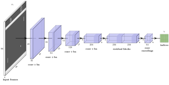
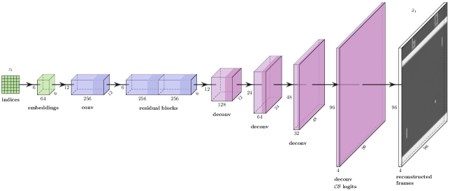
Figure 2: Visualization of the observation encoder architecture (top) and decoder architecture (bottom).

Dynamics.

For the recurrent dynamics we use a two-cell convolutional LSTM (Shi et al., 2015) with layer normalization. The input consists of a $6\times 6\times 48$ tensor, where the first $32$ channels are the embedding vectors looked up in the codebook of the VQ-VAE using the indices of the $6\times 6$ state representation. The last $16$ channels contain one-hot encodings of the actions, repeated along the spatial dimensions. By doing this, we condition the dynamics on the action. The action encodings are also concatenated to the output of each convolutional LSTM cell, since the action information might get lost during the forward pass. After the last convolutional LSTM cell, this corresponds to the intermediate representation $y_{t}$ from Fig. 1, which means that we actually drop its direct dependence on $z_{t}$. Then, there are two prediction heads, one for the next latent variable, $f_{\phi}(y_{t})$ consisting of one convolutional layer, and one for the reward, $g_{\phi}(y_{t})$ consisting of a convolutional layer and two fully-connected layers. The convolutional layers are followed by layer normalization and leaky ReLU nonlinearities. For a detailed depiction of the model see Fig. 3.

The output of $f_{\phi}(y_{t})$ is a $H\times W\times K$ tensor (${6\times 6\times 128}$) that contains the unnormalized scores for the embedding indices that get normalized via the softmax function,

$$p_{\phi}\!\left(z_{t+1}^{(j,k)}\,\middle|\,y_{t}\right)=\operatorname{Cat}\!\left(K,\,\operatorname{Softmax}\!\left(f_{\phi}^{(j,k)}(y_{t})\right)\right)\!.$$ (5)

We suppose that the discretization of the latent space stabilizes the dynamics model, since it has to predict scores for a predefined set of categories instead of real values, especially considering that the target is moving, i.e., the latent representations change during training.

The rewards are discretized into three categories $\{-1,0,1\}$ by clipping them into the interval $[-1,1]$ and rounding them to the nearest integer. The output of ${g_{\phi}(y_{t})}$ is a $3$-dimensional vector containing the scores for each reward category, which are also normalized via the softmax function,

$$p_{\phi}(r_{t}|y_{t})=\operatorname{Cat}\!\left(3,\operatorname{Softmax}\!\left(g_{\phi}(y_{t})\right)\right)\!.$$ (6)

The support of this distribution is ${r\in\{1,2,3\}}$, so we have to map the rewards accordingly (${r=r_{\text{orig}}+2}$) when we compute the likelihood.

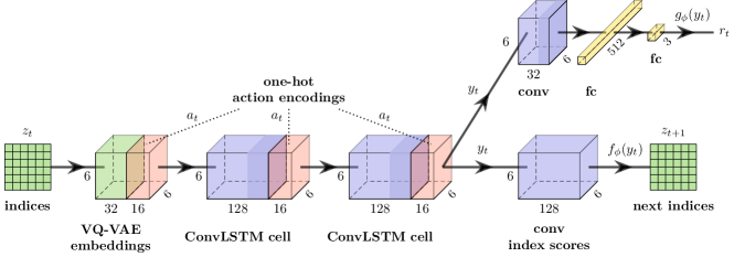
Figure 3: A visualization of the architecture of the dynamics network. After the second convolutional LSTM cell the network splits into the reward prediction head $g_{\phi}(y_{t})$ at the top and the next latent prediction head $f_{\phi}(y_{t})$ at the bottom. The recurrent states $h_{t},h_{t-1}$ of the LSTM are not visualized for clarity.

Policy.

The input of the policy network are the embedding vectors and it processes them using two convolutional layers with layer normalization, followed by a fully connected layer. Unlike Eq. 4 the policy does not depend on the recurrent variable $h_{t-1}$ from the world model in our experiments, but this could be useful for more complex environments. The output of the network ${f_{\theta}(z_{t})}$ is again a vector of unnormalized scores of a categorical distribution for the $M$ possible actions,

$$p_{\theta}(a_{t}|z_{t})=\operatorname{Cat}\!\left(M,\operatorname{Softmax}\!\left(f_{\theta}(z_{t})\right)\right)\!.$$ (7)

Table 2: Number of parameters of the world model compared with Kaiser et al. (2020) (their number is approximate).

Model	# parameters
Ours	$10332740$
SimPLe	$74000000$

Number of Parameters.

Table 2 shows the number of parameters of our model compared with the model by Kaiser et al. (2020), which uses about seven times as many parameters. Table 3 shows the number of parameters of our models in detail. At training time all models are used, but at test time only the encoder and the policy network are required.

3.4 Training

The distributions in Eq. 5 and Eq. 6 are trained using maximum likelihood. The policy is optimized on simulated experience using proximal policy optimization (Schulman et al., 2017), a model-free reinforcement learning algorithm. We approximate the expectations in Eq. 1 and Eq. 2 with single Monte Carlo samples. While we simulate experience, we use the same sample ${z_{t}\sim p(z_{t}|x_{t})}$ for both the dynamics, Eq. 3, and the policy, Eq. 2. At inference time, when the policy is applied to a real environment, Eq. 2 still needs access to the observation encoder ${p_{\phi}(z_{t}|x_{t})}$ in order to sample the latent variables.

Table 3: Number of parameters of our models in detail. The encoder and decoder both need access to the embedding vectors, therefore the sum of their individual number of parameters is slightly higher than for the total VQ-VAE.

Model	# parameters
World model	$10332740$
VQ-VAE	$4089313$
Encoder	$2014720$
Decoder	$2078689$
Dynamics network	$6243427$
Policy network	$1297415$
World model + policy (training)	$11630155$
Encoder + policy (inference)	$3312135$

Episodic Environments.

Atari games are episodic, therefore the world model needs to predict terminal states, for instance by predicting a binary variable that indicates the end of the episode. This prediction has to be reliable, since an incorrect prediction of “true” can have a severe impact on the simulated experience and thus on the policy.

We follow Kaiser et al. (2020) and end all episodes after a fixed number of steps (e.g., 50), so the world model does not have to terminate episodes.

Furthermore, we adopt the idea of randomly selecting the initial observation of a simulated episode from the collected real data. This enables the policy to learn from experience from any stage of the environment, although the number of time steps is limited. On the downside, this prevents the policy to learn from effects that are longer than the fixed number of steps (Kaiser et al., 2020).

Iterative Training.

We adopt the iterative training procedure from Kaiser et al. (2020) and alternate between interacting with the real environment, training the world model, and training the policy.

We also adopt the number of interactions per iteration, $6400$, and the number of iterations, $15$. The authors state that they perform additional $6400$ interactions prior to the first iteration. Thus, we perform $12800$ interactions in the first iteration, resulting in the same number of total interactions, ${$12800$+$6400$\times$14$=$102400$}$. In the first iteration we use a random uniform policy.

Warming Up Latent Representations.

After collecting the first batch of data, we train the VQ-VAE separately for $50$ epochs with a higher learning rate. We want to give the dynamics model a better starting point, with representations that already contain useful information. This cannot be done in later training stages, as the dynamics model would not be able to keep up with the representations.

Fixed Representations.

After warming up, we even slow down the state representation training by updating the parameters of the VQ-VAE only in every second training step, so the targets of the dynamics model are moving slower.

Reward Loss.

If the gradients coming from the reward prediction head have a high magnitude, they have a degrading effect on the performance of the next latent prediction head. We solve this issue by scaling down the cross-entropy loss of the rewards to reduce its influence on the entire model, but using a higher learning rate for the reward prediction head to compensate for the smaller gradients.

Constant KL Term.

Kaiser et al. (2020) state that the weight of the KL divergence loss of a variational autoencoder is game dependent, which makes VAEs impractical to apply on all Atari games without fine-tuning. The VQ-VAE does not suffer from this problem, since the KL term is constant and depends on the number of embeddings.

(a) Freeway

(b) Gravitar

(c) Hero

Figure 4: Mean episode reward across five training runs for three Atari environments. The x-axis shows the number of interactions with the real environment, and does not reflect the number of parameter updates that were performed in between. For SimPLe (Kaiser et al., 2020) we only know the final score which is depicted by a straight line.

4 Evaluation

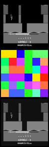
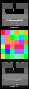
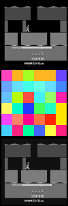
(a) Hero

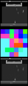
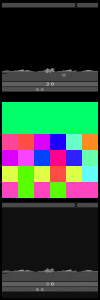
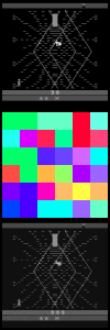
(b) Krull

Figure 5: Visualization of original game frames (top row), the encoded $6\times 6$ discrete latent variables (middle row), and the reconstructions from the VQ-VAE (bottom row). We assign colors to the embedding indices and draw a colored square for each entry of the latent matrix. A square does not necessarily correspond to the same area in the frame as they have larger receptive fields.

We compare our method with the variant of Kaiser et al. (2020) (stochastic discrete, 50 steps, $\gamma=0.99$) that comes closest to our model in terms of hyperparameters (discount rate, batch size etc.) and number of parameter updates.

This implies that the results of Kaiser et al. (2020) that are shown are not necessarily the best across all of their variants, but the best for a fairer comparison with our method. We do not know the performance difference to Kaiser et al. (2020) in terms of training time and test time, but considering the model size our method should be a lot faster.

We restrict our agent to $100K$ interactions with the environment and average the results over five training runs. For every run we evaluate the latest policy in each iteration by rolling out $32$ episodes in the real environment and computing the mean of the (cumulative) episode rewards. In Table 4 we report the mean final episode rewards (i.e., the mean episode reward after the final iteration; averaged over five runs) for $36$ Atari environments. Our method achieves a higher value than SimPLe (Kaiser et al., 2020) in $20$ out of $36$ environments (when also considering no frame stacking, as explained below).

Learning Curves.

Fig. 4 shows three cases of learning curves that were typical for our model. First, Fig. 4(a) shows an example of an environment in which the agent’s performance successfully increases over the course of training. Secondly, Fig. 4(b) shows an example of an environment in which the agent’s performance decreases over the course of training. This can have various reasons, e.g., when the agent reaches a new area of the state space and the environment dynamics change drastically. Finally, Fig. 4(c) shows an example of an environment in which the agent has comparably high performance starting from the first iteration, which is most likely due to model bias.

Latent Representations.

In Fig. 5 we can see that the state representation model is able to encode almost all information into the latent representation. However, the embedding indices are tuned for the decoder, so the dynamics model still has a hard task. We picked these two environments to show that changes in the scene (Fig. 5(a)) or even switching scenes (Fig. 5(b)) can be represented, although this can cause some loss of details (e.g., see the left reconstruction in Fig. 5(b)).

No Frame Stacking.

Our default model stacks the last four frames to incorporate short-time information into the state representations. On the downside, this introduces complexity, since the same frame can get a different representation, depending on the three other frames in the stack. This in turn will make it harder for the dynamics model to predict the next representation. The results show that no frame stacking improves the performance in some environments, as can be seen in Table 4.

Exploration.

In our experiments we observe the same phenomenon as Kaiser et al. (2020), namely that the results can vary drastically for different runs with the same hyperparameters but different random seeds. The main reasons might be that the world model cannot infer dynamics of regions of the environment’s state space that it has never seen before, and that the algorithm is very sensitive to the exploration-exploitation trade-off, as the number of interactions is low.

Table 4: Comparison of our method (with and without frame stacking) with SimPLe (Kaiser et al., 2020) and model-free PPO (Schulman et al., 2017) trained with $100K$ steps. Our scores are the mean final episode reward, averaged over five runs $\pm$ standard deviation. The PPO scores are taken from Kaiser et al. (2020).

	Ours (4 frames)		Ours (1 frame)		SimPLe (SD, $\gamma=0.99$)		PPO $100K$
Game	Mean	Std. Dev.	Mean	Std. Dev.	Mean	Std. Dev.	Mean	Std. Dev.
Alien	$409.9$	$(\pm\,73.0)$	$\mathbf{423.3}$	$(\pm\,48.1)$	$405.2$	$(\pm\,130.8)$	$291.0$	$(\pm\,40.3)$
Amidar	$37.6$	$(\pm\,13.6)$	$30.5$	$(\pm\,10.1)$	$\mathbf{88.0}$	$(\pm\,23.8)$	$56.5$	$(\pm\,20.8)$
Assault	$375.4$	$(\pm\,111.9)$	$408.3$	$(\pm\,27.8)$	$369.3$	$(\pm\,107.8)$	$\mathbf{424.2}$	$(\pm\,55.8)$
Asterix	$504.4$	$(\pm\,53.3)$	$456.5$	$(\pm\,146.4)$	$\mathbf{1089.5}$	$(\pm\,335.3)$	$385.0$	$(\pm\,104.4)$
Asteroids	$862.9$	$(\pm\,85.4)$	$989.9$	$(\pm\,88.7)$	$731.0$	$(\pm\,165.3)$	$\mathbf{1134.0}$	$(\pm\,326.9)$
Atlantis	$9413.1$	$(\pm\,3349.8)$	$15463.7$	$(\pm\,5478.7)$	$14481.6$	$(\pm\,2436.9)$	$\mathbf{34316.7}$	$(\pm\,5703.8)$
BankHeist	$101.2$	$(\pm\,17.4)$	$\mathbf{249.3}$	$(\pm\,49.8)$	$8.2$	$(\pm\,4.4)$	$16.0$	$(\pm\,12.4)$
BattleZone	$\mathbf{5631.2}$	$(\pm\,1179.1)$	$5531.3$	$(\pm\,2515.4)$	$5184.4$	$(\pm\,1347.5)$	$5300.0$	$(\pm\,3655.1)$
BeamRider	$410.4$	$(\pm\,55.4)$	$527.6$	$(\pm\,61.8)$	$422.7$	$(\pm\,103.6)$	$\mathbf{563.6}$	$(\pm\,189.4)$
Bowling	$27.9$	$(\pm\,4.8)$	$24.5$	$(\pm\,5.1)$	$\mathbf{34.4}$	$(\pm\,16.3)$	$17.7$	$11.2$
Boxing	$-2.8$	$(\pm\,5.7)$	$-9.3$	$(\pm\,12.6)$	$\mathbf{9.1}$	$(\pm\,8.8)$	$-3.9$	$(\pm\,6.4)$
Breakout	$8.8$	$(\pm\,1.5)$	$8.4$	$(\pm\,1.5)$	$\mathbf{12.7}$	$(\pm\,3.8)$	$5.9$	$(\pm\,3.3)$
ChopperCommand	$766.2$	$(\pm\,195.3)$	$590.6$	$(\pm\,335.0)$	$\mathbf{1246.9}$	$(\pm\,392.0)$	$730.0$	$(\pm\,199.0)$
CrazyClimber	$\mathbf{47536.9}$	$(\pm\,6114.9)$	$36923.8$	$(\pm\,2780.6)$	$39827.8$	$(\pm\,22582.6)$	$18400.0$	$(\pm\,5275.1)$
DemonAttack	$195.0$	$(\pm\,76.4)$	$\mathbf{211.3}$	$(\pm\,86.2)$	$169.5$	$(\pm\,41.8)$	$192.5$	$(\pm\,83.1)$
FishingDerby	$-89.6$	$(\pm\,4.5)$	$\mathbf{-87.9}$	$(\pm\,4.1)$	$-91.5$	$(\pm\,2.8)$	$-95.6$	$(\pm\,4.3)$
Freeway	$\mathbf{24.6}$	$(\pm\,3.4)$	$11.3$	$(\pm\,9.6)$	$20.3$	$(\pm\,18.5)$	$8.0$	$(\pm\,9.8)$
Frostbite	$214.4$	$(\pm\,10.2)$	$219.1$	$(\pm\,45.6)$	$\mathbf{254.7}$	$(\pm\,4.9)$	$174.0$	$(\pm\,40.7)$
Gopher	$687.2$	$(\pm\,91.1)$	$\mathbf{1398.4}$	$(\pm\,166.5)$	$771.0$	$(\pm\,160.2)$	$246.0$	$(\pm\,103.3)$
Gravitar	$87.2$	$(\pm\,60.9)$	$82.2$	$(\pm\,64.5)$	$198.3$	$(\pm\,39.9)$	$\mathbf{235.0}$	$(\pm\,197.2)$
Hero	$3453.6$	$(\pm\,594.7)$	$\mathbf{3911.6}$	$(\pm\,1259.3)$	$1295.1$	$(\pm\,1600.1)$	$569.0$	$(\pm\,1100.9)$
IceHockey	$-13.6$	$(\pm\,2.5)$	$-12.0$	$(\pm\,2.1)$	$-10.5$	$(\pm\,2.2)$	$\mathbf{-10.0}$	$(\pm\,2.1)$
Jamesbond	$66.6$	$(\pm\,7.8)$	$46.6$	$(\pm\,24.2)$	$\mathbf{125.3}$	$(\pm\,112.5)$	$65.0$	$(\pm\,46.4)$
Kangaroo	$245.0$	$(\pm\,99.6)$	$276.3$	$(\pm\,136.7)$	$\mathbf{323.1}$	$(\pm\,359.8)$	$140.0$	$(\pm\,102.0)$
Krull	$3520.2$	$(\pm\,211.4)$	$3241.0$	$(\pm\,448.4)$	$\mathbf{4539.9}$	$(\pm\,2470.4)$	$3750.4$	$(\pm\,3071.9)$
KungFuMaster	$11903.1$	$(\pm\,4399.5)$	$8521.2$	$(\pm\,1330.9)$	$\mathbf{17257.2}$	$(\pm\,5502.6)$	$4820.0$	$(\pm\,983.2)$
MsPacman	$652.2$	$(\pm\,92.6)$	$668.3$	$(\pm\,86.4)$	$\mathbf{762.8}$	$(\pm\,331.5)$	$496.0$	$(\pm\,379.8)$
NameThisGame	$\mathbf{2448.4}$	$(\pm\,179.5)$	$2119.4$	$(\pm\,217.9)$	$1990.4$	$(\pm\,284.7)$	$2225.0$	$(\pm\,423.7)$
Pong	$\mathbf{11.8}$	$(\pm\,6.9)$	$-3.9$	$(\pm\,7.6)$	$5.2$	$(\pm\,9.7)$	$-20.5$	$(\pm\,0.6)$
PrivateEye	$\mathbf{99.4}$	$(\pm\,1.2)$	$96.9$	$(\pm\,5.4)$	$58.3$	$(\pm\,45.4)$	$10.0$	$(\pm\,20.0)$
Qbert	$480.9$	$(\pm\,143.5)$	$\mathbf{617.5}$	$(\pm\,149.5)$	$559.8$	$(\pm\,183.8)$	$362.5$	$(\pm\,117.8)$
Riverraid	$2100.2$	$(\pm\,50.4)$	$\mathbf{2273.3}$	$(\pm\,188.5)$	$1587.0$	$(\pm\,818.0)$	$1398.0$	$(\pm\,513.8)$
RoadRunner	$1562.5$	$(\pm\,440.2)$	$1723.8$	$(\pm\,688.2)$	$\mathbf{5169.4}$	$(\pm\,3939.0)$	$1430.0$	$(\pm\,760.0)$
Seaquest	$458.1$	$(\pm\,155.7)$	$\mathbf{531.5}$	$(\pm\,105.1)$	$370.9$	$(\pm\,128.2)$	$370.0$	$(\pm\,103.3)$
UpNDown	$1128.2$	$(\pm\,247.6)$	$1354.6$	$(\pm\,741.4)$	$2152.6$	$(\pm\,1192.4)$	$\mathbf{2874.0}$	$(\pm\,1105.8)$
YarsRevenge	$4096.0$	$(\pm\,520.9)$	$4360.3$	$(\pm\,1156.9)$	$2980.2$	$(\pm\,778.6)$	$\mathbf{5182.0}$	$(\pm\,1209.3)$

LSTM architecture.

Instead of a convolutional LSTM, we also tried follow-up architectures like the spatio-temporal LSTM (Wang et al., 2017) or causal LSTM (Wang et al., 2018), but for our problem the performance gain was not significant enough, compared with the imposed additional training time and number of parameters.

5 Limitations and Future Work

Currently, our dynamics model samples the indices in the latent representation independently. This might be disadvantageous because conditional dependencies between the indices, which correspond to certain areas of the video frames, are ignored. So in the future it would be interesting to predict them autoregressively, e.g., with a conditional PixelCNN (van den Oord et al., 2016) conditioned on $y_{t}$, to see whether this solves prediction errors like duplication or incoherent movement of objects. Nevertheless, an autoregressive model might have a negative impact on the training times (when training the dynamics model and when simulating experience), and it has to be seen whether the resulting training times are acceptable.

Another line of research should improve exploration in order to enable even higher sample efficiency. Furthermore, we would like the world model to predict terminal states and move away from terminating episodes after a fixed number of steps, since this introduces a new hyperparameter that needs to be tuned, and prevents the agent from learning beyond this time horizon.

6 Conclusion

In this paper we demonstrate that a generative model with a discrete latent space can be used to strongly decrease the size of world models. We employ a VQ-VAE with a discrete two-dimensional latent space. We show that this powerful model is able to effectively encode the complex visual observations of Atari games. The chosen model and latent space have produced representations that are more stable and expressive at the same time. Our experiments show that acting entirely in latent space is possible, which speeds up training since no decoding into high-dimensional frames is required.

References

- Babaeizadeh et al. (2017) Babaeizadeh, M., Finn, C., Erhan, D., Campbell, R. H., and Levine, S. Stochastic variational video prediction. arXiv preprint arXiv:1710.11252, 2017.
- Bishop (1994) Bishop, C. M. Mixture density networks. Technical report, Aston University, Birmingham, 1994.
- Ha & Schmidhuber (2018) Ha, D. and Schmidhuber, J. Recurrent world models facilitate policy evolution. In Bengio, S., Wallach, H., Larochelle, H., Grauman, K., Cesa-Bianchi, N., and Garnett, R. (eds.), Advances in Neural Information Processing Systems 31, pp. 2450–2462. Curran Associates, Inc., 2018.
- Hafner et al. (2020a) Hafner, D., Lillicrap, T., Ba, J., and Norouzi, M. Dream to control: Learning behaviors by latent imagination. arXiv preprint arXiv:1912.01603, 2020a.
- Hafner et al. (2020b) Hafner, D., Lillicrap, T., Norouzi, M., and Ba, J. Mastering atari with discrete world models. arXiv preprint arXiv:2010.02193, 2020b.
- Kaiser et al. (2020) Kaiser, L., Babaeizadeh, M., Miłos, P., Osiński, B., Campbell, R. H., Czechowski, K., Erhan, D., Finn, C., Kozakowski, P., Levine, S., Mohiuddin, A., Sepassi, R., Tucker, G., and Michalewski, H. Model based reinforcement learning for atari. In International Conference on Learning Representations, 2020.
- Kingma & Welling (2014) Kingma, D. P. and Welling, M. Auto-encoding variational bayes. In Bengio, Y. and LeCun, Y. (eds.), 2nd International Conference on Learning Representations, ICLR 2014, Banff, AB, Canada, April 14-16, 2014, Conference Track Proceedings, 2014.
- Loaiza-Ganem & Cunningham (2019) Loaiza-Ganem, G. and Cunningham, J. P. The continuous bernoulli: fixing a pervasive error in variational autoencoders. In Wallach, H., Larochelle, H., Beygelzimer, A., d'Alché-Buc, F., Fox, E., and Garnett, R. (eds.), Advances in Neural Information Processing Systems 32, pp. 13287–13297. Curran Associates, Inc., 2019.
- Schulman et al. (2017) Schulman, J., Wolski, F., Dhariwal, P., Radford, A., and Klimov, O. Proximal policy optimization algorithms. arXiv preprint arXiv:1707.06347, 2017.
- Shi et al. (2015) Shi, X., Chen, Z., Wang, H., Yeung, D.-Y., Wong, W.-k., and WOO, W.-c. Convolutional lstm network: A machine learning approach for precipitation nowcasting. In Cortes, C., Lawrence, N. D., Lee, D. D., Sugiyama, M., and Garnett, R. (eds.), Advances in Neural Information Processing Systems 28, pp. 802–810. Curran Associates, Inc., 2015.
- van den Oord et al. (2016) van den Oord, A., Kalchbrenner, N., Vinyals, O., Espeholt, L., Graves, A., and Kavukcuoglu, K. Conditional image generation with pixelcnn decoders, 2016.
- van den Oord et al. (2017) van den Oord, A., Vinyals, O., and kavukcuoglu, k. Neural discrete representation learning. In Guyon, I., Luxburg, U. V., Bengio, S., Wallach, H., Fergus, R., Vishwanathan, S., and Garnett, R. (eds.), Advances in Neural Information Processing Systems 30, pp. 6306–6315. Curran Associates, Inc., 2017.
- Wang et al. (2017) Wang, Y., Long, M., Wang, J., Gao, Z., and Yu, P. S. Predrnn: Recurrent neural networks for predictive learning using spatiotemporal lstms. In Guyon, I., Luxburg, U. V., Bengio, S., Wallach, H., Fergus, R., Vishwanathan, S., and Garnett, R. (eds.), Advances in Neural Information Processing Systems 30, pp. 879–888. Curran Associates, Inc., 2017.
- Wang et al. (2018) Wang, Y., Gao, Z., Long, M., Wang, J., and Philip, S. Y. PredRNN++: Towards a resolution of the deep-in-time dilemma in spatiotemporal predictive learning. In International Conference on Machine Learning, pp. 5123–5132, 2018.