Layer-wise Guided Training for BERT:
Learning Incrementally Refined Document Representations

Abstract

Although bert is widely used by the nlp community, little is known about its inner workings. Several attempts have been made to shed light on certain aspects of bert, often with contradicting conclusions. A much raised concern focuses on bert’s over-parameterization and under-utilization issues. To this end, we propose o novel approach to fine-tune bert in a structured manner. Specifically, we focus on Large Scale Multilabel Text Classification (lmtc) where documents are assigned with one or more labels from a large predefined set of hierarchically organized labels. Our approach guides specific bert layers to predict labels from specific hierarchy levels. Experimenting with two lmtc datasets we show that this structured fine-tuning approach not only yields better classification results but also leads to better parameter utilization.

1 Introduction

Despite bert’s (Devlin et al., 2019) popularity and effectiveness, little is known about its inner workings. Several attempts have been made to demystify certain aspects of bert (Rogers et al., 2020), often leading to contradicting conclusions. For instance, Clark et al. (2019) argue that attention measures the importance of a particular word when computing the next level representation for this word. However, Kovaleva et al. (2019) showed that most attention heads contain trivial linguistic information and follow a vertical pattern (attention to [cls], [sep], and punctuation tokens), which could be related to under-utilization or over-parameterization issues. Other studies attempted to link specific bert heads with linguistically interpretable functions (Htut et al., 2019; Clark et al., 2019; Kovaleva et al., 2019; Voita et al., 2019; Hoover et al., 2020; Lin et al., 2019), agreeing that no single head densely encodes enough relevant information but instead different linguistic features are learnt by different attention heads. We hypothesize that the aforementioned largely contributes to the lack of attention-based explainability of bert. Another open topic is how the knowledge is distributed across bert layers. Most studies agree that syntactic knowledge is gathered in the middle layers (Hewitt and Manning, 2019; Goldberg, 2019; Jawahar et al., 2019), while the final layers are more task-specific. Most importantly, it seems that any semantic knowledge is spread across the model, explaining why non-trivial tasks are better solved at the higher layers (Tenney et al., 2019).

Driven by the above discussion, we propose a novel fine-tuning approach where different parts of bert are guided to directly solve increasingly challenging classification tasks following an underlying label hierarchy. Specifically, we focus on Large Scale Multilabel Text Classification (lmtc) where documents are assigned with one or more labels from a large predefined set. The labels are organized in a hierarchy from general to specific concepts. Our approach attempts to tie specific bert layers with specific hierarchy levels. In effect, each of these layers is responsible for predicting the labels of the corresponding level. We experiment with two lmtc datasets (eurlex57k, mimic-iii) and several variations of structured bert training. Our contributions are: (a) We propose a novel structured approach to fine-tune bert where specific layers are tied to specific hierarchy levels; (b) We show that structured training yields better results than the baseline across all levels of the hierarchy, while also leading to better parameter utilization.

Figure 1: The five variants of bert-based multi-label classifiers including the flat one and the four structured editions. The circles represent the classification layers attached to [cls] tokens across layers.

2 Datasets

eurlex57k Chalkidis et al. (2019) contains 57k eu legal acts from eurlex. Each act is approx. 700 words long and is annotated with one or more concepts from eurovoc which contains 7,391 concepts organized in an 8-level hierarchy. We truncate the hierarchy to 6 levels by discarding the last 2 levels which contain 50 rarely used labels.

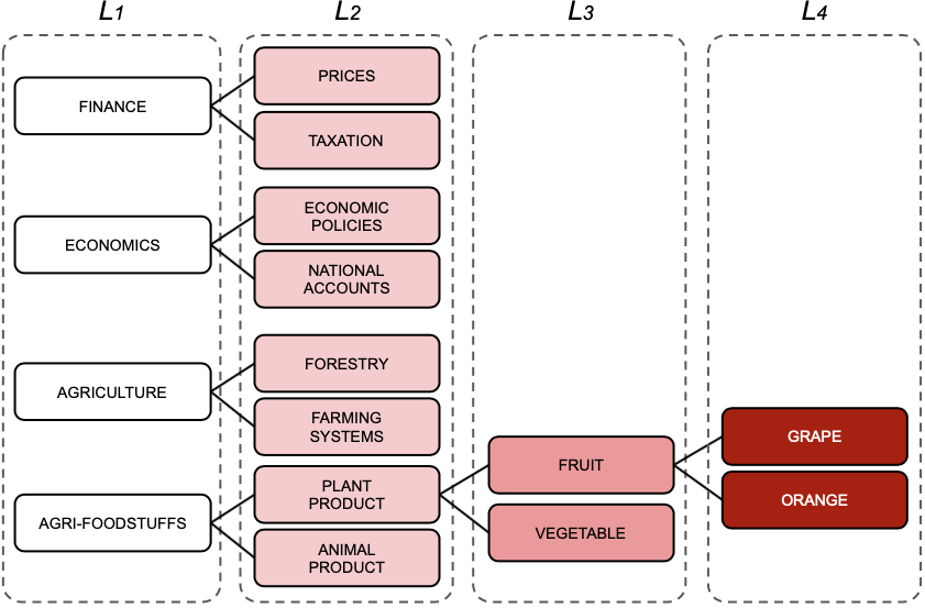
Figure 2: Examples from eurovoc label hierarchy. Layer-wise models consider all labels in the same level ($L_{i}$; dashed boxes) of the hierarchy on-par.

mimic-iii Johnson et al. (2017) contains approx. 52k discharge summaries from us hospitals. Each summary is approx. 1.6k words long and is annotated with one or more icd-9 codes. icd-9 contains 22,395 codes organized in a 7-level hierarchy. We truncate the hierarchy to 6 levels, discarding the first level which contains only 4 general codes.³

Label Augmentation: In both datasets, we make the assumption that if a label $l$ is assigned to a document then all of its ancestors should also be assigned to this document. Hence, we augment labels by annotating a document with all the ancestors of its assigned labels. For instance, in eurovoc, if a document is annotated with the label grape it will also be annotated with grape’s ancestors, i.e., fruit, plant product, and agri-foodstuffs (Figure 2). This assumption is perfectly valid, while also having the added side effect of providing a more accurate test-bed for evaluation. For example, if a classifier mistakenly annotated the document with citrus fruit, a sibling of grape, in the non-augmented case it would receive a score of zero. By contrast, in the augmented case, assuming it correctly identified all the ancestors of citrus fruit it would receive a much higher score of 0.75 having correctly assigned the three ancestors of grape but not the (more specialized) label itself. Thus, we believe the model is evaluated more fairly in the augmented case with respect to the hierarchy. This type of evaluation is also in-line with the literature on hierarchical classification Kosmopoulos et al. (2015).

Labels Depth	1	2	3	4	5	6	Micro	Macro
eurlex- bert-base
#Labels	21	127	567	3,861	2,284	481	7,341	7,341
flat	90.3 $\pm$ 0.2	83.9 $\pm$ 0.3	81.0 $\pm$ 0.5	74.8 $\pm$ 1.0	74.5 $\pm$ 1.2	79.9 $\pm$ 1.4	80.6 $\pm$ 0.6	80.7 $\pm$ 0.6
last-six	90.7 $\pm$ 0.1	84.6 $\pm$ 0.0	81.9 $\pm$ 0.2	76.8 $\pm$ 0.2	77.2 $\pm$ 0.5	82.2 $\pm$ 1.1	81.7 $\pm$ 0.1	82.2 $\pm$ 0.1
one-by-one	90.0 $\pm$ 0.0	84.3 $\pm$ 0.1	81.7 $\pm$ 0.2	76.2 $\pm$ 0.2	76.7 $\pm$ 0.5	81.6 $\pm$ 0.2	81.3 $\pm$ 0.1	81.7 $\pm$ 0.0
in-pairs	89.9 $\pm$ 0.2	84.3 $\pm$ 0.2	81.7 $\pm$ 0.2	76.7 $\pm$ 0.3	77.2 $\pm$ 0.6	81.7 $\pm$ 0.4	81.4 $\pm$ 0.1	81.9 $\pm$ 0.4
hybrid	90.5 $\pm$ 0.2	84.3 $\pm$ 0.1	81.7 $\pm$ 0.2	76.6 $\pm$ 0.4	76.6 $\pm$ 0.7	81.8 $\pm$ 0.7	81.5 $\pm$ 0.2	81.9 $\pm$ 0.0
mimic-iii- scibert
#Labels	79	589	3,982	9,640	7,234	867	22,391	22,391
flat	75.5 $\pm$ 0.0	66.5 $\pm$ 0.2	57.7 $\pm$ 0.4	50.8 $\pm$ 0.4	43.2 $\pm$ 0.8	38.6 $\pm$ 3.3	60.1 $\pm$ 0.4	55.4 $\pm$ 0.9
last-six	76.8 $\pm$ 0.2	67.3 $\pm$ 0.1	58.5 $\pm$ 0.1	51.2 $\pm$ 0.0	43.8 $\pm$ 0.3	40.9 $\pm$ 0.1	60.4 $\pm$ 0.0	56.4 $\pm$ 0.1
one-by-one	75.7 $\pm$ 0.0	66.7 $\pm$ 0.1	57.9 $\pm$ 0.1	50.6 $\pm$ 0.1	43.4 $\pm$ 0.3	41.8 $\pm$ 0.6	59.8 $\pm$ 0.1	56.0 $\pm$ 0.2
in-pairs	75.6 $\pm$ 0.1	66.5 $\pm$ 0.1	58.1 $\pm$ 0.1	50.9 $\pm$ 0.1	43.6 $\pm$ 0.3	40.9 $\pm$ 0.8	59.9 $\pm$ 0.1	55.9 $\pm$ 0.2
hybrid	76.4 $\pm$ 0.1	67.0 $\pm$ 0.1	58.5 $\pm$ 0.1	51.3 $\pm$ 0.0	43.8 $\pm$ 0.2	40.0 $\pm$ 0.4	60.3 $\pm$ 0.0	56.2 $\pm$ 0.1

Table 1: $\mathrm{R}$-$\mathrm{Precision}$ $\pm$ std for all variants of bert-base on eurlex and mimic-iii test data across hierarchy depths.

3 Structured Learning with BERT

Before we proceed with the description of our methods (Figure 1), we introduce some notation. Given a label hierarchy $L$ of depth $d$, $L_{n}$ denotes the set of labels in the $n^{\mathrm{th}}$ level of this hierarchy ($n\leqslant d$). Also, $f_{i}=\sigma(W_{i}\cdot c_{i}+b_{i})$ is a classification function, where $W_{i}$ and $b_{i}$ are trainable parameters, $c_{i}$ is the [cls] token in the $i^{\mathrm{th}}$ bert layer, and $\sigma$ is the sigmoid activation function. Note that the sizes of $W_{i}$ and $b$ depend on the number of labels that $f_{i}$ is responsible for predicting, i.e., if $f_{i}$ predicts the labels of $L_{n}$, $W_{i}\in\mathbb{R}^{|L_{n}|\times 768}$ and $b_{i}\in\mathbb{R}^{|L_{n}|\times 1}$.

flat: This is a simple baseline which uses $f_{12}$ to predict all labels in the hierarchy in a flat manner. In effect, $W_{12}\in\mathbb{R}^{|L|\times 768}$ and $b_{i}\in\mathbb{R}^{|L|\times 1}$. Note that this model achieves state-of-the-art results on eurlex57k but not on mimic-iii Chalkidis et al. (2020). However, our results are not directly comparable to Chalkidis et al. (2020) because our methods operate on augmented label sets.

last-six: This method uses the classifiers $f_{7}$ through $f_{12}$ to predict the labels in $L_{1}$ through $L_{6}$, respectively. Our intuition is that the layers 1-6 will retain and enhance their pre-trained functionality, i.e., syntactic knowledge, contextualized representations, while layers 7-12 will leverage this knowledge to better solve their individual tasks. We also expect that the model will show higher parameter utilization for the layers 7-12 since they are forced to solve gradually more refined classification tasks.

one-by-one: This method utilizes the full depth of bert in a “skip one, use one” fashion, i.e., it uses classifiers $f_{i}$, $i\in\{2,4,\dots,12\}$. In effect, the odd layers ($1,3,\dots,11$) are updated only indirectly, through the classification tasks of the even layers. We expect that the odd layers will learn rich latent representations to facilitate the classifiers of the even layers. Spreading the classification tasks across the whole depth of the model will potentially lead to better parameter utilization. On the other hand, it could harm the model’s pre-trained functionality and hence its performance.

in-pairs: This method also exploits the full depth of bert, but now the layers are grouped in 6 pairs, $p_{n}\in\{(1,2),(3,4),\dots,(11,12)\}$. The classifier responsible for the labels of $L_{n}$ operates on the concatenated [cls] tokens of the corresponding pair, e.g., $f_{1}=\sigma(W_{1}\cdot[c_{1};c_{2}]+b_{1})$ is trained on the labels of $L_{1}$. We expect in-pairs to have better parameter utilization than one-by-one, although the risk of hindering performance is now even higher.

hybrid: Similarly to last-six, this method skips some of the lower bert layers (3 instead of 6). Also, it ties $L_{1}$, $L_{2}$, and $L_{6}$, which are the hierarchy levels with the fewest labels to layers 4, 5, and 12, respectively. Finally, similarly to in-pairs the remaining bert layers are grouped in pairs and are tied to the rest of the hierarchy levels. We expect the first three layers to retain and enhance their pre-trained functionality, while the hierarchy levels with a large number of labels will benefit from the additional parameters at their disposal.

Figure 3: Angular distance between [cls] representations across layers.

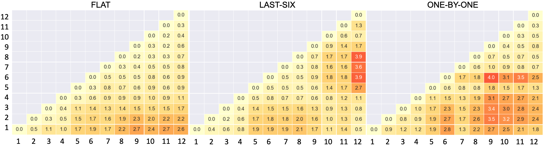
Figure 4: $\mathrm{KL}$-$\mathrm{Divergence}$ between attention distributions across layers.

Layer	1		2		3		4		5		6		7		8		9		10		11		12
flat	4.7	1.3	3.9	0.7	2.5	0.9	3.6	1.7	3.3	2.6	3.2	3.2	3.4	3.1	2.7	2.6	2.1	2.1	2.6	1.8	2.2	1.2	2.4	0.6
last-six	4.6	1.5	4.2	0.6	4.1	0.8	3.9	1.1	2.7	2.7	2.9	3.6	2.9	3.0	2.6	2.9	3.0	4.2	4.5	3.9	4.3	2.3	5.2	0.6
one-by-one	4.5	1.9	4.1	2.4	4.0	4.7	4.0	3.8	3.7	4.2	2.8	2.9	4.6	2.7	4.0	3.0	3.9	1.7	3.9	1.8	4.4	1.4	4.5	0.2
in-pairs	4.4	1.9	3.9	3.0	3.9	4.6	4.1	4.2	3.2	3.6	3.5	3.5	4.1	2.5	3.5	2.8	3.7	2.0	3.7	1.4	4.2	1.1	5.1	0.2
hybrid	4.6	2.0	4.5	0.9	4.2	1.7	4.2	2.1	3.8	3.4	3.1	3.7	4.1	3.8	3.8	3.6	4.1	2.8	4.3	2.5	4.1	1.1	4.7	0.3

Table 2: $\mathrm{Entropy}$ (left column) and $\mathrm{KL}$-$\mathrm{Divergence}$ (right column) of attention distributions per layer.

4 Experiments

We report $\mathrm{R}$-$\mathrm{Precision}$ Manning et al. (2009) at each hierarchy level as well as micro (flat) and macro averages across all levels. Table 1 shows the results in both datasets. In eurlex57k our structured methods always outperform the baseline mostly by a large margin. last-six achieves the best overall results and is superior than the other structured methods in all hierarchy levels indicating that allowing the lower layers to retain and enhance their pre-trained functionality is crucial. Similar observations can be made for mimic-iii, but in this case the importance of not damaging bert’s pre-trained functionality is even higher, as evident by the only minor improvements one-by-one and in-pairs have compared to flat.

5 Discussion on model utilization

Comparing [cls] representations: Figure 3 shows the average angular distances between the [cls] representations of each layer on development data of eurlex57k. The angular distance is calculated on unit ($\mathrm{L}_{2}$ normalized) vectors, takes values in $[0,1]$, and a distance of 0.5 indicates an angle of $90^{\circ}$. We observe that one-by-one leads to larger angles between the representations than last-six which in turn yields larger angles than flat. In effect, one-by-one and to a lesser extent last-six lead to a better parameter utilization than flat. To better support this claim we provide a geometric interpretation. We first $\mathrm{L}_{2}$ normalize all [cls] representations. Each normalized representation can be interpreted as a vector having its initial point at the origin and its terminal point at the surface of a 768-dimensional hyper-sphere (centered at the origin). The larger the angle between two [cls] vectors the further apart they are on the hyper-sphere’s surface. Effectively, [cls] vectors with large angles between them cover a larger sub-area of the hyper-sphere’s surface indicating that the vector space is utilized to a higher extent which directly implies better parameter utilization.

Comparing attention distributions: Figure 4 shows the $\mathrm{KL}$-$\mathrm{Divergence}$ of the average (across heads) attention for all layers on the development data of eurlex57k.⁸ A high $\mathrm{KL}$-$\mathrm{Divergence}$ indicates that two layers attend to different sub-word units. Moreover, Table 2 reports the entropy (left column per layer) of the average (across heads) attention distribution per layer. A high entropy indicates that a layer attends to more sub-word units. Table 2 also reports the average $\mathrm{KL}$-$\mathrm{Divergence}$ (right column per layer) between the attention distributions of each possible pair of heads in a layer. A high $\mathrm{KL}$-$\mathrm{Divergence}$ indicates that each head attends to different sub-word units. A first observation is that flat attends to almost the same sub-word units across layers (small entropy differences and $\mathrm{KL}$-$\mathrm{Divergence}$ across layers). Interestingly, the different attention heads focus on different sub-word units only in the middle layers (5-8). On the other hand, all the structured methods show better utilization of the attention mechanism, having higher entropy and $\mathrm{KL}$-$\mathrm{Divergence}$ both across heads (Table 2) and across layers (Figure 4).

6 Related Work

Our approach is similar to Wehrmann et al. (2018) but they experiment with fully connected networks, which are not well suited for text classification, contrary to stacked transformers (Vaswani et al., 2017; Devlin et al., 2019). Similarly, Yan et al. (2015) used Convolutional Neural Networks, albeit with shallow hierarchies (2 levels). Although our approach leverages the label hierarchy it should not be confused with hierarchical classification methods (Silla and Freitas, 2011), which typically employ one classifier per node and cannot scale-up to large hierarchies when considering neural classifiers. A notable exception is the work of You et al. (2019) who employed one bidirectional lstm with label-wise attention (You et al., 2018) per hierarchy node. However, for their method to scale-up, they use probabilistic label trees (Khandagale et al., 2019) to organize the labels in their own shallow hierarchy which does not follow the abstraction level of the original hierarchy. To the best of our knowledge we are the first to apply this approach to pre-trained language models.

7 Conclusions and Further Work

We proposed a novel guided approach to fine-tune bert, where specific layers are tied to specific hierarchy levels. Experimenting with two lmtc datasets, we showed that structured training not only yields better results than a flat baseline, but also leads to better parameter utilization. In the future we will try to further increase the parameter utilization by guiding bert’s attention heads to explicitly focus on specific hierarchy parts. We also plan to improve the explainability of our methods with respect to the utilization of their parameters.

Appendix A Data manipulation

Hierarchy truncation: In order to directly apply all our methods, we truncate both hierarchies and reduce their depth to six. We believe this truncation is justified since in eurovoc the last two layers contain a very small number of labels, which are rarely, if at all, assigned and in icd-9 the first layer also contains a very small number of labels which are very general and can be trivially classified (Table 3). In both cases it seems that only minimal information is lost which would have small practical use in the classification tasks.

Depth	eurovoc	icd-9
1	21	4*
2	127	79
3	568	589
4	4,545	3,982
5	2,335	9,640
6	497	7,234
7	79*	867
8	6*	-
Overall	8,178 / 8,093	22,395 / 22,391

Table 3: Label distribution across eurovoc and icd-9 hierarchy levels. Concepts (labels) are arranged from more abstract (level 1-2) to more specialized ones (levels 6-8). Labels with an asterisk are truncated in our experiments.

Document Truncation: Documents in both datasets are often above the 512 token limit of bert. To reduce document size, we perform a number of pre-processing normalizations, including removal of numeric tokens, punctuation and stop-words. In eurlex documents have been tokenized using SpaCy’s default tokenizer, while in mimic-iii, we use regular expressions tailored for the biomedical domain. While document length is severely reduced post normalization, if a document still has a larger number of tokens, i.e. more than 512, we use the first 512 tokens and ignore the rest.

Appendix B Experimental Setup

All our methods build on bert-base and are implemented in Tensorflow 2. For eurlex we use the original bert-base (Devlin et al., 2019), while for mimic-iii we use scibert (Beltagy et al., 2019), which has the same architecture (12 layers, 768 hidden units, 12 attention heads), and better suits biomedical documents. Our models are tuned by grid searching three learning rates ($2\mathrm{e}\text{-}5,3\mathrm{e}\text{-}5,5\mathrm{e}\text{-}5$) and two drop-out rates ($0,0.1$). We use the Adam optimizer Kingma and Ba (2015) with early stopping on validation loss. In preliminary experiments, we found that weighting individual losses with respect to the number of labels in each level is crucial. We therefore weigh each loss by the percentage of labels at the corresponding level, i.e., $w_{n}=\frac{|L_{n}|}{|L|}$, where $|L_{n}|$ is the number of labels in the $n^{\mathrm{th}}$ level of the hierarchy and $|L|$ is the total number of labels across all levels, e.g., in eurlex57k, $w_{1}=\frac{21}{8093}\approx 0.0026$.

Appendix C Evaluation in LMTC

The literature of lmtc Rios and Kavuluru (2018); Chalkidis et al. (2019) mostly uses information retrieval evaluation measures. We support the premise that when the number of labels is that large the problem mimics retrieval with each document acting as a query and the model having to score relevant labels higher than the rest. However in our study, it would be really confusing to report the standard retrieval metrics $\mathrm{Recall}@R$, $\mathrm{Precision}@K$, $\mathrm{nDCG}@K$ since we evaluate our classifiers at each hierarchy depth and reasonable values for $K$ have large fluctuations between levels, as the number of labels per level vastly varies (see Table 3). Instead, we prefer $\mathrm{R}$-$\mathrm{Precision}$ Manning et al. (2009), which is the $\mathrm{Precision}@R$ where $R$ is the number of gold labels associated with each document. It follows that $\mathrm{R}$-$\mathrm{Precision}$ can neither under-estimate (penalize) nor over-estimate the performance of the models Chalkidis et al. (2019).

Appendix D Peculiarities of mimic-iii dataset

In our experiments we observe a hindered performance in mimic-iii, which can be attributed to a number of characteristics of the dataset. Firstly, documents contain a lot of non-trivial biomedical terminology which naturally makes the classification task more difficult. Further, discharge summaries describe a patient’s condition during their hospitalization and therefore proper label annotations change throughout the document as the patient’s diagnosis changes or as they exhibit new symptoms, e.g., “the patient was admitted to the hospital with no heart issues, […] the patient had a heart failure and died.”. Both the in-domain language and the constant change of events make the dataset more challenging than eurlex57k, where documents are more organized and well-written also with simpler language.

It therefore seems reasonable that in mimic-iii allowing lower bert layers to retain and enhance the preliminary functionality, without explicitly guiding them, is of utmost importance. We would like to highlight that even though we use scibert (Beltagy et al., 2019), which is based on a new scientific vocabulary, we observe that specialized biomedical terms are often over-fragmented in multiple sub-word units, e.g. ‘atelectasis’ splits into [‘ate’, ‘##lect’, ‘##asis’]. Thus, the initial layers need to decipher these over-fragmented sub-word units and reconstruct the original word semantics. On the contrary, in eurlex57k, classifying general concepts in the initial layers, even considering only the sub-word unit embeddings is plausible.

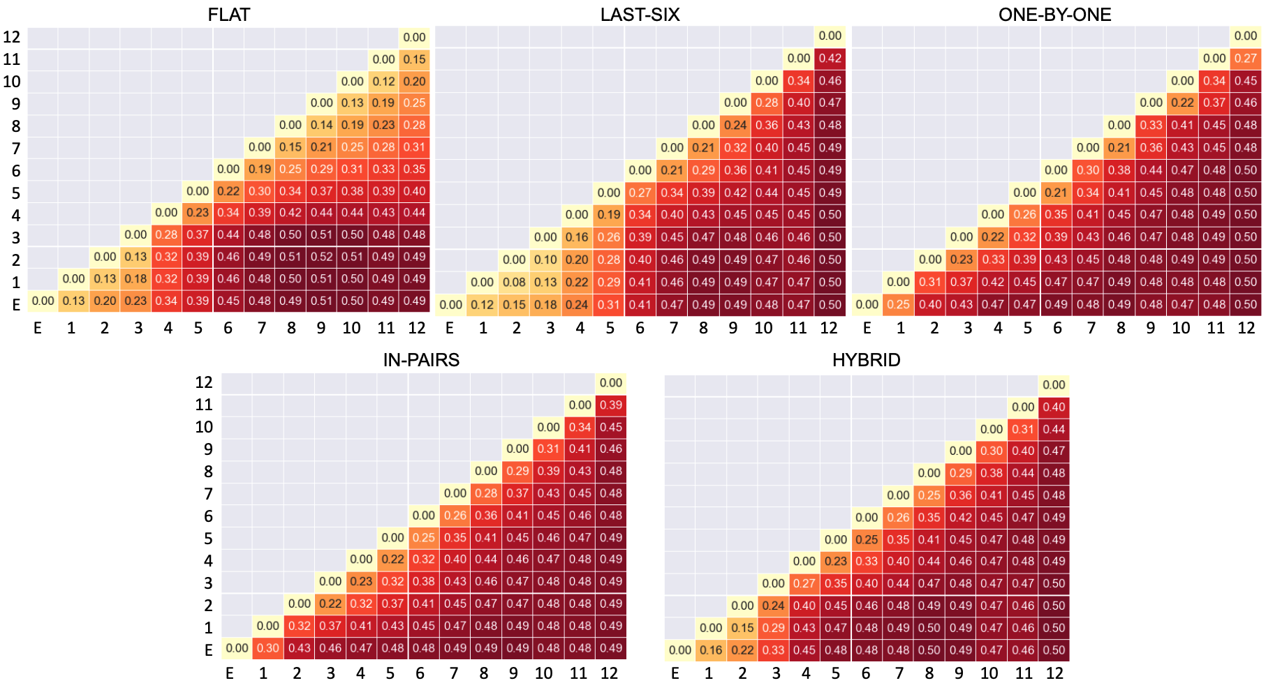
Figure 5: Angular distance between [cls] representations across layers in the development dataset of eurlex57k.

Figure 6: $\mathrm{KL}$-$\mathrm{Divergence}$ between attention distributions across layers in the development dataset of eurlex57k.

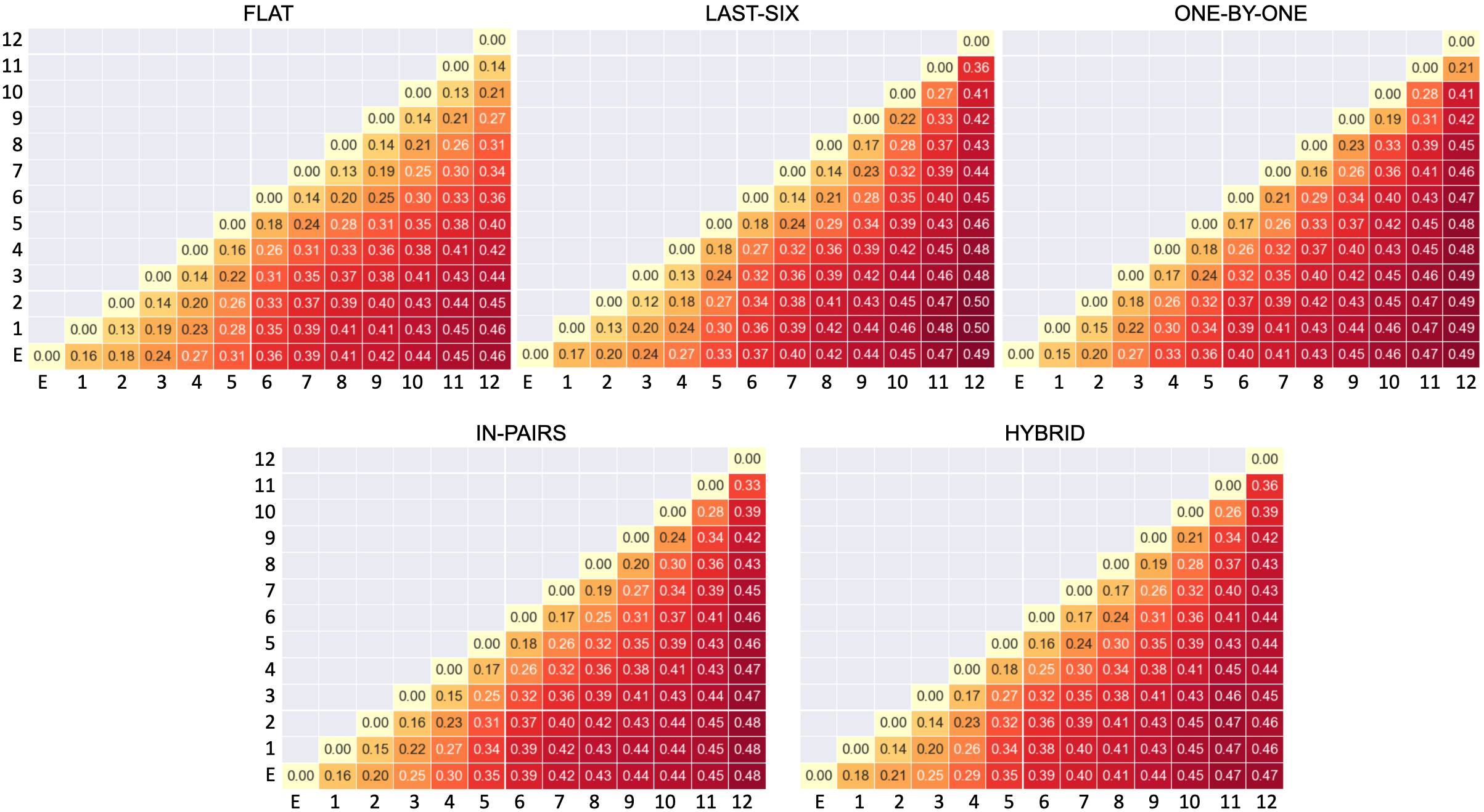
Figure 7: Angular distance between [cls] representations across layers in the development dataset of mimic-iii.

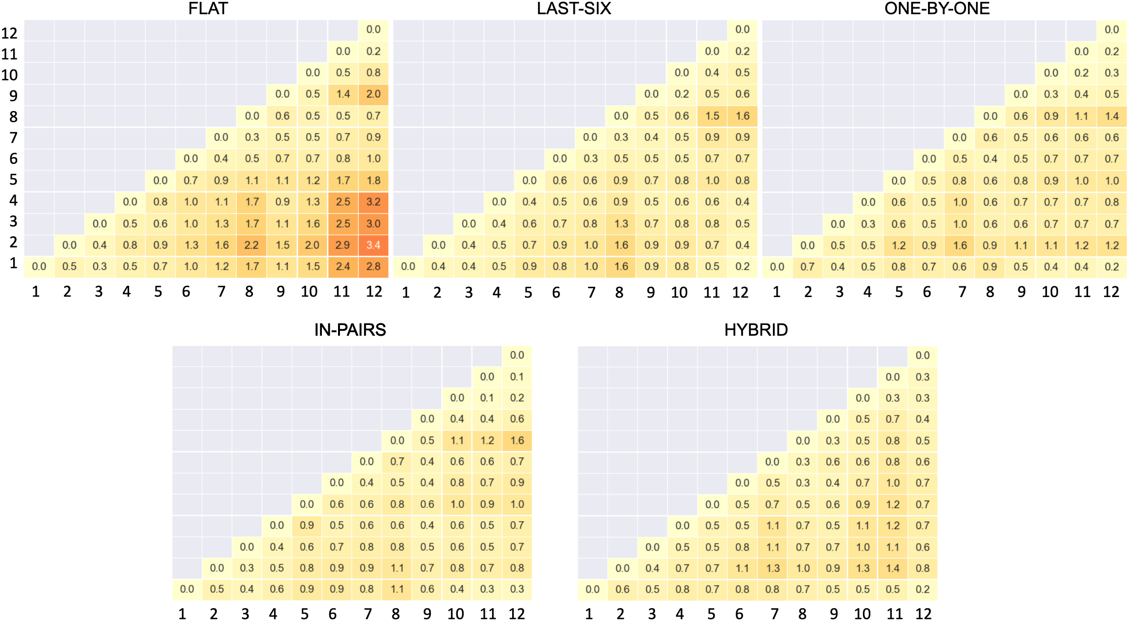
Figure 8: $\mathrm{KL}$-$\mathrm{Divergence}$ between attention distributions across layers in the development dataset of mimic-iii.

Appendix E Discussion on model utilization

We present additional results for the rest of the methods (in-pairs, hybrid). Figure 5 shows the average angular distances between the [cls] representations of each layer (Figure 5) for all considered methods. We observe that the distances of in-pairs between consecutive [cls] representations follow a similar pattern with those of one-by-one, with the exception of 0.25+ distances which are more dense in the upper layers for in-pairs. This is reasonable, since in in-pairs all layers directly contribute to the classification tasks. The pattern of hybrid is very similar to one-by-one and in-pairs, except for the first three non-guided layers in which distances bear close resemblance to those of the corresponding layers in last-six. Similar observations hold for mimic-iii (Figure 7). Finally, Figure 6 shows the $\mathrm{KL}$-$\mathrm{Divergence}$ of the average (across heads) attention for all layers on the development data. All structured methods show better utilization of the attention mechanism than flat, having higher $\mathrm{KL}$-$\mathrm{Divergence}$ across layers. Contrary, in mimic-iii, all structured methods follow a similar pattern of low $\mathrm{KL}$-$\mathrm{Divergence}$ across layers (Figure 8), even lower than the upper layers of flat, i.e., the models attend to similar sub-word positions across layers. We aim to further study and explain this behaviour in future work.

References

- Beltagy et al. (2019) Iz Beltagy, Kyle Lo, and Arman Cohan. 2019. SciBERT: A pretrained language model for scientific text. In Proceedings of the 2019 Conference on Empirical Methods in Natural Language Processing and the 9th International Joint Conference on Natural Language Processing (EMNLP-IJCNLP), pages 3606–3611, Hong Kong, China.
- Chalkidis et al. (2019) Ilias Chalkidis, Emmanouil Fergadiotis, Prodromos Malakasiotis, and Ion Androutsopoulos. 2019. Large-Scale Multi-Label Text Classification on EU Legislation. In Proceedings of the 57th Annual Meeting of the Association for Computational Linguistics, pages 6314–6322, Florence, Italy.
- Chalkidis et al. (2020) Ilias Chalkidis, Manos Fergadiotis, Sotiris Kotitsas, Prodromos Malakasiotis, Nikolaos Aletras, and Ion Androutsopoulos. 2020. An empirical study on large-scale multi-label text classification including few and zero-shot labels.
- Clark et al. (2019) Kevin Clark, Urvashi Khandelwal, Omer Levy, and Christopher D. Manning. 2019. What does BERT look at? an analysis of BERT’s attention. In Proceedings of the 2019 ACL Workshop BlackboxNLP: Analyzing and Interpreting Neural Networks for NLP, pages 276–286, Florence, Italy. Association for Computational Linguistics.
- Devlin et al. (2019) Jacob Devlin, Ming-Wei Chang, Kenton Lee, and Kristina Toutanova. 2019. BERT: Pre-training of Deep Bidirectional Transformers for Language Understanding. Proceedings of the Annual Conference of the North American Chapter of the Association for Computational Linguistics: Human Language Technologies, abs/1810.04805.
- Goldberg (2019) Yoav Goldberg. 2019. Assessing bert’s syntactic abilities.
- Hewitt and Manning (2019) John Hewitt and Christopher D. Manning. 2019. A structural probe for finding syntax in word representations. In Proceedings of the 2019 Conference of the North American Chapter of the Association for Computational Linguistics: Human Language Technologies, Volume 1 (Long and Short Papers), pages 4129–4138, Minneapolis, Minnesota. Association for Computational Linguistics.
- Hoover et al. (2020) Benjamin Hoover, Hendrik Strobelt, and Sebastian Gehrmann. 2020. exBERT: A Visual Analysis Tool to Explore Learned Representations in Transformer Models. In Proceedings of the 58th Annual Meeting of the Association for Computational Linguistics: System Demonstrations, pages 187–196, Online. Association for Computational Linguistics.
- Htut et al. (2019) Phu Mon Htut, Jason Phang, Shikha Bordia, and Samuel R. Bowman. 2019. Do attention heads in bert track syntactic dependencies?
- Jawahar et al. (2019) Ganesh Jawahar, Benoît Sagot, and Djamé Seddah. 2019. What does BERT learn about the structure of language? In Proceedings of the 57th Annual Meeting of the Association for Computational Linguistics, pages 3651–3657, Florence, Italy. Association for Computational Linguistics.
- Johnson et al. (2017) Alistair EW Johnson, David J. Stone, Leo A. Celi, and Tom J. Pollard. 2017. MIMIC-III, a freely accessible critical care database. Nature.
- Khandagale et al. (2019) Sujay Khandagale, Han Xiao, and Rohit Babbar. 2019. Bonsai - Diverse and Shallow Trees for Extreme Multi-label Classification. CoRR, abs/1904.08249.
- Kingma and Ba (2015) Diederik P. Kingma and Jim Ba. 2015. Adam: A method for stochastic optimization. In Proceedings of the 5th International Conference on Learning Representations.
- Kosmopoulos et al. (2015) Aris Kosmopoulos, Ioannis Partalas, Eric Gaussier, Georgios Paliouras, and Ion Androutsopoulos. 2015. Evaluation measures for hierarchical classification: a unified view and novel approaches. Data Mining and Knowledge Discovery, 29(3):820–865.
- Kovaleva et al. (2019) Olga Kovaleva, Alexey Romanov, Anna Rogers, and Anna Rumshisky. 2019. Revealing the dark secrets of BERT. In Proceedings of the 2019 Conference on Empirical Methods in Natural Language Processing and the 9th International Joint Conference on Natural Language Processing (EMNLP-IJCNLP), pages 4365–4374, Hong Kong, China. Association for Computational Linguistics.
- Lin et al. (2019) Yongjie Lin, Yi Chern Tan, and Robert Frank. 2019. Open sesame: Getting inside BERT’s linguistic knowledge. In Proceedings of the 2019 ACL Workshop BlackboxNLP: Analyzing and Interpreting Neural Networks for NLP, pages 241–253, Florence, Italy. Association for Computational Linguistics.
- Manning et al. (2009) Christopher D. Manning, Prabhakar Raghavan, and Hinrich Schütze. 2009. Introduction to Information Retrieval. Cambridge University Press.
- Rios and Kavuluru (2018) Anthony Rios and Ramakanth Kavuluru. 2018. Few-Shot and Zero-Shot Multi-Label Learning for Structured Label Spaces. In Proceedings of the 2018 Conference on Empirical Methods in Natural Language Processing, pages 3132–3142. Association for Computational Linguistics.
- Rogers et al. (2020) Anna Rogers, Olga Kovaleva, and Anna Rumshisky. 2020. A primer in bertology: What we know about how bert works. arXiv preprint arXiv:2002.12327.
- Silla and Freitas (2011) Carlos N Silla and Alex A Freitas. 2011. A survey of hierarchical classification across different application domains. Data Mining and Knowledge Discovery, 22(1-2):31–72.
- Tenney et al. (2019) Ian Tenney, Dipanjan Das, and Ellie Pavlick. 2019. BERT rediscovers the classical NLP pipeline. In Proceedings of the 57th Annual Meeting of the Association for Computational Linguistics, pages 4593–4601, Florence, Italy. Association for Computational Linguistics.
- Vaswani et al. (2017) Ashish Vaswani, Noam Shazeer, Niki Parmar, Jakob Uszkoreit, Llion Jones, Aidan N. Gomez, Lukasz Kaiser, and Illia Polosukhin. 2017. Attention Is All You Need. In 31th Annual Conference on Neural Information Processing Systems, Long Beach, CA, USA.
- Voita et al. (2019) Elena Voita, David Talbot, Fedor Moiseev, Rico Sennrich, and Ivan Titov. 2019. Analyzing multi-head self-attention: Specialized heads do the heavy lifting, the rest can be pruned. In Proceedings of the 57th Annual Meeting of the Association for Computational Linguistics, pages 5797–5808, Florence, Italy. Association for Computational Linguistics.
- Wehrmann et al. (2018) Jonatas Wehrmann, Ricardo Cerri, and Rodrigo Barros. 2018. Hierarchical multi-label classification networks. In Proceedings of the 35th International Conference on Machine Learning, volume 80 of Proceedings of Machine Learning Research, pages 5075–5084, Stockholmsmässan, Stockholm Sweden. PMLR.
- Yan et al. (2015) Zhicheng Yan, Hao Zhang, Robinson Piramuthu, Vignesh Jagadeesh, Dennis DeCoste, Wei Di, and Yizhou Yu. 2015. Hd-cnn: Hierarchical deep convolutional neural networks for large scale visual recognition. In 2015 IEEE International Conference on Computer Vision (ICCV), pages 2740–2748.
- You et al. (2018) Ronghui You, Suyang Dai, Zihan Zhang, Hiroshi Mamitsuka, and Shanfeng Zhu. 2018. Attentionxml: Extreme multi-label text classification with multi-label attention based recurrent neural networks. arXiv preprint arXiv:1811.01727.
- You et al. (2019) Ronghui You, Zihan Zhang, Ziye Wang, Suyang Dai, Hiroshi Mamitsuka, and Shanfeng Zhu. 2019. Attentionxml: Label tree-based attention-aware deep model for high-performance extreme multi-label text classification. In Advances in Neural Information Processing Systems 32, pages 5812–5822. Curran Associates, Inc.