Shadow, deflection angle and quasinormal modes of Born-Infeld charged black holes

Abstract

In this paper, we consider black holes in the consistent Aoki-Gorji-Mukohyama theory of the four-dimensional Einstein-Gauss-Bonnet (4D EGB) gravity in the presence of Born-Infeld (BI) nonlinear electrodynamics. We study several optical features of these black holes such as the shadow radius, energy emission rate and deflection angle, and analyse the effect of the coupling constants, the electric charge and cosmological constant on the considered optical quantities. Furthermore, we also employ the connection between the shadow radius and quasinormal modes (QNMs) and investigate small scalar perturbations around the black hole solution. We show that the variation of the parameters of the theory provide specific signatures on the optical features of the BI charged black hole solution, thus leading to the possibility of directly testing this consistent Aoki-Gorji-Mukohyama 4D EGB black hole model by using astrophysical observations.

I Introduction

Recently, a novel four-dimensional Einstein-Gauss-Bonnet (4D EGB) gravity was proposed by Glavan and Lin EGB0 by rescaling the Gauss-Bonnet (GB) coupling $\alpha\rightarrow\tilde{\alpha}/(D-4)$, and then defining the four-dimensional theory as the limit $D\rightarrow 4$, at the level of the field equations. In this manner, the GB term yields a non-trivial contribution to the gravitational dynamics. It has also been discussed whether this regularized theory is reliable EGB17a ; EGB17b ; EGB17c ; EGB17d ; EGB18 ; Arrechea:2020evj ; Gurses:2020rxb ; Arrechea:2020gjw and several remedies have been suggested to overcome the objections raised EGB18 ; EGB20 ; EGB21 ; EGB22 . It is worthwhile to mention that these theories still hold the spherically symmetric 4D black holes as valid solutions EGB20 ; EGB21 . In Aoki:2020lig , the consistent Aoki-Gorji-Mukohyama theory of 4D EGB gravity was proposed and several applications were further studied in Aoki:2020iwm ; Aoki:2020ila . In fact, the novel 4D EGB theory of gravity has recently attracted much attention in a wide context of black hole physics Fernandes:2020rpa ; Konoplya:2020qqh ; Kumar:2020uyz ; Kumar:2020xvu ; Zhang:2020qew ; Shaymatov:2020yte , and applications, such as, in black hole shadows Konoplya:2020bxa ; Guo:2020zmf ; EslamPanah:2020hoj ; Zeng:2020dco , thermodynamics issues Hegde:2020xlv ; Singh:2020xju , rotating solutions Kumar:2020owy ; Wei:2020ght ; Konoplya:2020fbx , stability issues Ghosh:2020vpc ; Konoplya:2020juj ; HosseiniMansoori:2020yfj ; Wei:2020poh ; Konoplya:2020cbv ; Zhang:2020sjh ; Aragon:2020qdc ; Liu:2020evp , gravitational lensing Islam:2020xmy , thin accretion disk around 4D EGB black holes Liu:2020vkh , causal structure Ge:2020tid ; Dadhich:2020ukj , and black hole solutions coupled to nonlinear electrodynamics (NLED) DVSingh ; Ghosh:2018bxg ; DVSingh ; Jusufi:2020qyw ; Jafarzade:2020ilt ; Yang:2020jno .

Motivated by recent astrophysical observations, namely, the first image of a supermassive black hole candidate in the center of M87 galaxy captured by the Event Horizon Telescope project KAkiyama1 ; KAkiyama2 , we are interested in performing an in-depth analysis of the optical features of black hole solutions. More specifically, we consider the solution obtained in 4D EGB gravity minimally coupled to Born-Infeld (BI) electrodynamics in the presence of a negative cosmological constant, provided in Yang:2020jno . In fact, BI electrodynamics is a well-known NLED theory, proposed by Born and Infeld in 1934 BornInfeld , in order to regularize the ultraviolet divergent self-energy of a point-like charge in classical dynamics. Moreover, it was shown later that this nonlinear theory may come from the low energy limit of open superstring theory fradkin1985effective ; metsaev1987born ; bergshoeff1987born . In addition, experiments of photon-photon interaction have proposed a nonlinear model for electrodynamics in vacuum nonlin1 ; nonlin2 ; nonlin3 ; nonlin4 ; nonlin5 . The effects of NLED from a cosmological viewpoint have been studied, for instance, in Vargas1a ; Vollick1a . It has also been shown that NLED theories can remove both the big bang and black hole singularities Corda1b ; DeLorenci ; Cuesta1a . The shadow of nonregular black holes in the presence of the Euler-Heisenberg NLED, which is effectively the low-energy limit of BI electrodynamics, has been determined in EHTM8 , and comparing the results with the ones of the M87 imaged by the Event Horizon Telescope Project, the first astrophysical constraints on nonlinear electrodynamics has been presented. Hence, it is a significant expectation that NLED may affect astrophysical characteristics such as the shadow radius of a charged black hole. In the context of 4D EGB gravity, several generalized solutions were obtained in the literature such as generalized Reissner-Nordstrom black hole with a Maxwell electric field coupling to the 4D EGB gravity Fernandes:2020rpa , Bardeen-like Kumar:2020uyz and Hayward-like Kumar:2020xvu black holes by interacting the new gravitational theory with nonlinear electrodynamics, and AdS black holes in the novel 4D EGB gravity coupled to exponential nonlinear electrodynamics DVSingh ; Ghosh:2018bxg ; Jafarzade:2020ilt . Thus, in this work, we specifically analyse the shadow geometrical shape, the energy emission rate, the deflection angle and quasinormal modes in the BI charged black hole solution obtained in Yang:2020jno . The behavior of photon orbits around black holes in the presence of a variety of nonlinear electrodynamics have also been studied in Xu:2019yub ; Habibina:2020msd . In addition to various theories of black holes, the effects of NLED theories would become quite important in super-strongly magnetized compact objects, such as pulsars, particular neutron stars, magnetars and strange quark magnetars Mosquera1a ; Mosquera1b ; Bialynicka1b .

This paper is organised in the following manner: In section II, we present the consistent Aoki-Gorji-Mukohyama action and the specific black hole solution of 4D EGB gravity minimally coupled to BI electrodynamics in the presence of a negative cosmological constant. In section III, we consider the motion of a free photon in the black hole background, and write out the specific condition for a circular null geodesic. Then, we analyse the photon sphere radius by varying the black hole parameters in subsection. We also consider the radius of the shadow and examine the effect of the model’s parameters and analyse the energy emission rate. In section IV, we study the connection between the radius of the shadow and quasinormal modes and consider small perturbations around the black holes. In section V, we consider the light deflection around the black hole solution. Finally, in section VI, we conclude by summarizing and discussing our results.

II Consistent Aoki-Gorji-Mukohyama theory of the 4D EGB theory and black hole solution

The consistent Aoki-Gorji-Mukohyama theory of 4D EGB gravity has been proposed in Aoki:2020lig and further perused in Aoki:2020iwm ; Aoki:2020ila . Since this consistent version of the theory does not respect time diffeomorphism, it is natural to use the $4$-dimensional Arnowitt-Deser-Misner (ADM) metric of the form

$$ds^{2}=-N^{2}dt^{2}+\gamma_{ij}(dx^{i}+N^{i}dt)(dx^{j}+N^{j}dt)\,,$$ (1)

where $N$, $N^{i}$ and $\gamma_{ij}$ are the lapse function, the shift vector and the spatial metric, respectively. The well-defined gravitational action in the presence of a negative cosmological constant is then given by Aoki:2020lig

$$S_{\mathrm{g}}=\frac{M_{\mathrm{Pl}}^{2}}{2}\int dtd^{3}xN\sqrt{\gamma}\left[-2\Lambda+2R-\mathcal{M}+\tilde{\alpha}R_{\mathrm{4DGB}}^{2}\right],$$ (2)

where

$$R_{\mathrm{4DGB}}^{2} \equiv \frac{1}{2}\Big{[}8R^{2}-4R\mathcal{M}-\mathcal{M}^{2}$$

$$-\frac{8}{3}\big{(}8R_{ij}R^{ij}-4R_{ij}\mathcal{M}^{ij}-\mathcal{M}_{ij}\mathcal{M}^{ij}\big{)}\Big{]},$$

in which

$$\mathcal{M}_{ij}\equiv R_{ij}+\mathcal{K}^{k}{}_{k}\mathcal{K}_{ij}-\mathcal{K}_{ik}\mathcal{K}^{k}{}_{j},\hskip 28.45274pt\mathcal{M}\equiv\mathcal{M}^{i}{}_{i}\,,$$

and

$$\mathcal{K}_{ij}\equiv\frac{1}{2N}(\dot{\gamma}_{ij}-2D_{(i}N_{j)}-\gamma_{ij}D^{2}\lambda_{\mathrm{GF}})\,.$$

Here, $M_{\mathrm{Pl}}=1/\sqrt{8\pi G}$ is the reduced Planck mass, $G$ is the Newton gravitational constant and $\tilde{\alpha}$ is the rescaled Gauss-Bonnet coupling constant. The factor $\lambda_{\mathrm{GF}}$ is the Lagrange multiplier related to a gauge-fixing constraint (we refer the reader to Ref. Aoki:2020lig for more details). In addition, $D_{i}$ is the covariant derivative compatible with the spatial metric and dot denotes the derivative with respect to $t$. We will also set $\Lambda$ to $-3/l^{2}$. One of the properties of the consistent Aoki-Gorji-Mukohyama theory introduced by the action (2) is that if a $D$-dimensional solution of EGB gravity has vanishing Weyl tensor of the spatial metric $\gamma_{ij}$ and the Weyl piece of $2K_{i[m\mid}K_{j\mid n]}$, where $K_{ij}=\frac{1}{2N}(\dot{\gamma}_{ij}-2D_{(i}N_{j)})$, the $D\rightarrow 4$ limit of this solution is a solution of the well-defined theory of 4D EGB theory as well Aoki:2020lig ; Aoki:2020iwm ; Aoki:2020ila . Furthermore, the action (2) presents a consistent 4D EGB theory uniquely up to a choice of the gauge-fixing constraint imposed by the Lagrange multiplier $\lambda_{\mathrm{GF}}$.

In this paper, our aim is to study optical features of Born-Infeld charged black hole solutions of the consistent Aoki-Gorji-Mukohyama theory of 4D EGB gravity. Therefore, we minimally couple the gravitational Lagrangian to the BI electrodynamics Lagrangian given by

$$\mathcal{L}_{BI}=4\beta^{2}\left(1-\sqrt{1+\frac{2F}{\beta^{2}}}\right).$$ (3)

where $F=\frac{1}{4}F_{\mu\nu}F^{\mu\nu}$, with $F_{\mu\nu}=\partial_{\mu}A_{\nu}-\partial_{\nu}A_{\mu}$ and $A_{\mu}$ is the potential. Here $\beta>0$ denotes the BI parameter which is the maximum of the electromagnetic field strength.

Our desired solution namely BI charged black hole solution of 4D EGB gravity, has already been obtained in Yang:2020jno . However, we need to show that this solution is a solution of the consistent Aoki-Gorji-Mukohyama theory (2). As pointed out above, we just need to confirm that the Weyl tensor of the spatial metric and Weyl piece of $2K_{i[m\mid}K_{j\mid n]}$ vanish for $D$-dimensional black hole solution of EGB gravity minimally coupled to BI electrodynamics. This solution is a static and spherically symmetric solution with just one metric function $f\left(r\right)$ Yang:2020jno ; Aiello:2004rz ; Zou:2010tv . Hence, we consider the general form of this kind of solution

$$ds^{2}=-f(r)dt^{2}+\frac{dr^{2}}{f(r)}+r^{2}d\Omega_{D-2}^{2},$$ (4)

where

$$d\mathbf{\Omega}_{D-2}^{2}=d\theta_{1}^{2}+\sum\limits_{i=2}^{D-2}d\theta_{i}^{2}\prod\limits_{j=1}^{i-1}\sin^{2}\left(\theta_{j}\right),$$

is the line element of $(D-2)$-dimensional unit sphere. Comparing metric (4) with ADM metric (1), one confirms that $N^{2}=f(r)$, $N^{i}=0$ and

$$\gamma_{ij}=\mathrm{diag}\left(\frac{1}{f(r)},r^{2},r^{2}\sin^{2}\left(\theta_{1}\right),r^{2}\sin^{2}\left(\theta_{1}\right)\sin^{2}\left(\theta_{2}\right),\cdots\right).$$

(5)

Consequently, the condition $2K_{i[m\mid}K_{j\mid n]}=0$ where $K_{ij}=\frac{1}{2N}(\dot{\gamma}_{ij}-2D_{(i}N_{j)})$ is automatically satisfied. Moreover, our calculations show that for a spatial metric $\gamma_{ij}$ of the form given in Eq. (5), the Weyl tensor also vanishes. Thus, the $D\rightarrow 4$ limit of any $D$-dimensional solution of EGB gravity of the form given in Eq. (4), including the BI one, is a solution of the consistent Aoki-Gorji-Mukohyama theory of 4D EGB gravity defined by (2) minimally coupled to matter fields as well.

Varying the total action with respect to the gauge field, $A_{\mu}$, provides the following equation of motion

$$\partial_{\mu}\left(\frac{\sqrt{-g}F^{\mu\nu}}{\sqrt{1+2F/\beta^{2}}}\right)=0\,.$$ (6)

With ansatz (4), one could immediately integrate the electrodynamics equation of motion (6) with the gauge field being $A=\Phi(r)dt$ and obtain

$$\Phi(r)=\frac{Q}{r}{~{}}_{2}F_{1}\left(\frac{1}{4},\frac{1}{2},\frac{5}{4},-\frac{Q^{2}}{\beta^{2}r^{4}}\right)\,,$$ (7)

for $D=4$, in which $Q$ is the electric charge and ${}_{2}F_{1}$ is the hypergeometric function. Then, the metric function $f\left(r\right)$ is given by Yang:2020jno

$$f(r) = 1+\frac{r^{2}}{2\alpha}\Bigg{\{}1\pm\Bigg{[}1+4\alpha\Bigg{(}\frac{2M}{r^{3}}-\frac{1}{l^{2}}$$ (8)

$$-\frac{2\beta^{2}}{3}\bigg{(}1-\sqrt{1+\frac{Q^{2}}{\beta^{2}r^{4}}}\bigg{)}-\frac{4Q}{3r^{3}}\Phi(r)\Bigg{)}\Bigg{]}^{\frac{1}{2}}\Bigg{\}}.$$

Equation (8) corresponds to two branches of solutions depending on the choice of the sign. It can be shown that the positive-sign branch reduces to a RN-AdS solution with a negative gravitational mass and imaginary charge, and only the negative-sign branch recovers the proper RN-AdS limit (we refer the reader to Ref. Yang:2020jno for more details). Thus, since only negative branch leads to a physically meaningful solution, we will limit our discussions to this branch of the solution.

III Null geodesics and photon sphere

In this section, we analyse the motion of a free photon in the black hole background (8). Due to the spherical symmetry of the spacetime, we consider that the motion is limited to the equatorial plane $\theta=\pi/2$, without a significant loss of generality. Thus, the Lagrangian for a photon can be expressed as

$$2\mathcal{L}=-f(r)\dot{t}^{2}+\frac{\dot{r}^{2}}{f(r)}+r^{2}\dot{\phi}^{2},$$ (9)

where the overdot denotes a derivative with respect to the affine parameter. Taking into account Eq. (9), the equations of motion are given by

$$\dot{t}=-\frac{p_{t}}{f(r)},\qquad\dot{r}=p_{r}f(r),\qquad\dot{\phi}=\frac{p_{\phi}}{r^{2}},$$ (10)

where $p$ is the generalized momentum defined by $p_{\mu}=\partial\mathcal{L}/\partial\dot{x}^{\mu}=g_{\mu\nu}\dot{x}^{\nu}$.

The Hamiltonian for this system reads

$$H=\frac{1}{2}g^{\mu\nu}p_{\mu}p_{\nu}=\frac{1}{2}\left[-\frac{p_{t}^{2}}{f(r)}+f(r)p_{r}^{2}+\frac{p_{\phi}^{2}}{r^{2}}\right]=0.$$ (11)

Since the Hamiltonian is independent of the coordinates $t$ and $\phi$, one can consider $p_{t}\equiv-E$ and $p_{\phi}\equiv L$ as constants of motion, where $E$ and $L$ are physically interpreted as the energy and angular momentum of the photon; note that $p_{r}$ is the radial momentum. Using the equations of motion and these two conserved quantities, one can rewrite the null geodesic equation as follows

$$\dot{r}^{2}+V_{\rm eff}(r)=0,$$ (12)

where the effective potential is

$$V_{\rm eff}(r)=f(r)\left[\frac{L^{2}}{r^{2}}-\frac{E^{2}}{f(r)}\right].$$ (13)

For a circular null geodesic, the effective potential satisfies the following conditions, simultaneously

$$V_{\rm eff}(r)|_{r=r_{p}}=0,\qquad\frac{\partial V_{\rm eff}(r)}{\partial r}\Big{|}_{r=r_{p}}=0.$$ (14)

The conditions (14) determine the photon sphere radius $(r_{p})$ and the critical angular momentum of the photon sphere $(L_{p})$. Note that the photon orbits are unstable and are determined by the condition $\partial^{2}V_{\rm eff}(r)/\partial r^{2}<0$. The second condition of Eq. (14) yields the following expression

$$\frac{4Q^{2}}{3}\left(2\beta^{2}r_{p}^{4}{~{}}-\frac{Q^{2}}{5}\right){{}_{2}F_{1}}\left(\frac{1}{4},\frac{1}{2},\frac{5}{4},-\frac{Q^{2}}{\beta^{2}r_{p}^{4}}\right)$$

$$+\beta^{2}r_{p}^{6}\Bigg{\{}\Bigg{[}1+4\alpha\Bigg{(}\frac{2M}{r_{p}^{3}}+\frac{\Lambda}{3}-\frac{2\beta^{2}}{3}\bigg{(}1-\sqrt{1+\frac{Q^{2}}{\beta^{2}r_{p}^{4}}}\bigg{)}$$

$$-\frac{4Q^{2}}{3r_{p}^{4}}{~{}}_{2}F_{1}\left(\frac{1}{4},\frac{1}{2},\frac{5}{4},-\frac{Q^{2}}{\beta^{2}r_{p}^{4}}\right)\Bigg{)}\Bigg{]}^{\frac{1}{2}}-\frac{3M}{r_{p}}\Bigg{\}}=0\,,$$ (15)

which we solve numerically to obtain the radius of photon sphere. The event horizon $(r_{e})$ and photon sphere radius $(r_{p})$ are listed in Table 1, by varying several of the black hole parameters. We note that increasing the electric charge, and the GB and BI parameters leads to a decrease in the event horizon and photon sphere radius. However, the BI parameter does not play a significant role in this case. The effect of cosmological constant is slightly different, as increasing this parameter from $-0.15$ to $-0.01$ results in a decrease of the photon sphere radius and an increase of the event horizon. A remarkable point regarding the GB parameter is that its increasing leads to an imaginary value for the event horizon, which is physically meaningless. This shows that specific constraints should be imposed on this parameter.

Table 1: The event horizon and photon sphere radius for the variation of the electric charge, $Q$, the BI parameter, $\beta$, the GB parameter, $\alpha$, and the cosmological constant, $\Lambda$, for $M=1$.

$Q$	$0.1$	$0.3$	$0.6$	$0.9$
$r_{e}(\alpha=\beta=0.2$, $\Lambda=-0.02$)	$1.84$	$1.80$	$1.63$	$1.30$
$r_{p}(\alpha=\beta=0.2$, $\Lambda=-0.02$)	$2.91$	$2.85$	$2.64$	$2.18$
$\alpha$	$0.2$	$0.5$	$0.8$	$0.9$
$r_{e}(Q=\beta=0.2$, $\Lambda=-0.02$)	$1.83$	$1.64$	$1.37$	$0.98+0.2I$
$r_{p}(Q=\beta=0.2$, $\Lambda=-0.02$)	$2.89$	$2.73$	$2.54$	$2.46$
$\beta$	$0.05$	$0.1$	$0.15$	$0.25$
$r_{e}(Q=\alpha=0.2$, $\Lambda=-0.02$)	$1.8291$	$1.8283$	$1.8281$	$1.8280$
$r_{p}(Q=\alpha=0.2$, $\Lambda=-0.02$)	$2.8774$	$2.8762$	$2.8760$	$2.8759$
$\Lambda$	$-0.01$	$-0.06$	$-0.1$	$-0.15$
$r_{e}$ ($\alpha=\beta=Q=0.2$)	$1.85$	$1.76$	$1.70$	$1.63$
$r_{p}$ ($\alpha=\beta=Q=0.2$)	$2.88$	$2.90$	$2.92$	$2.94$

As a next step in the analysis, we examine the behavior of the shadow radius in the corresponding NLED theory coupled to EGB gravity. From the definition of the shadow radius Perlick1 , the size of black hole shadow can be expressed in celestial coordinates $(x,y)$ as

$$r_{s}=\sqrt{x^{2}+y^{2}}=\frac{L_{p}}{E}=\frac{r_{p}}{\sqrt{f(r_{p})}}.$$ (16)

Thus, using Eq. (16) and the listed values of Table 1, we explore the shadow size of this solution. To inspect the influence of the black hole parameters on the shadow geometric circular shape, we plot Fig. 1. Evidently, the electric charge decreases the shadow size for fixed values of $\alpha$, $\beta$ and $\Lambda$ (see Fig. 1(a)). Taking into account Figs. 1(b) and 1(e), we verify that the GB and BI parameters have a decreasing effect on the shadow radius similar to the electric charge. However, the variation of the BI parameter $\beta$ does not affect the shadow size significantly. Figure 1(c) depicts the impact of the cosmological constant on the size of the shadow. As we see, unlike the previous parameters, the cosmological constant increases the shadow radius and has a notable effect on it.

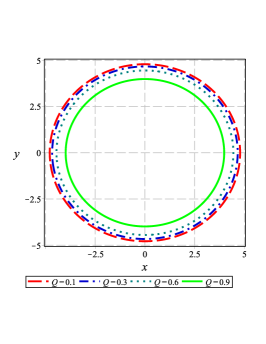
(a)  $\alpha=\beta=0.2$ and $\Lambda=-0.02$

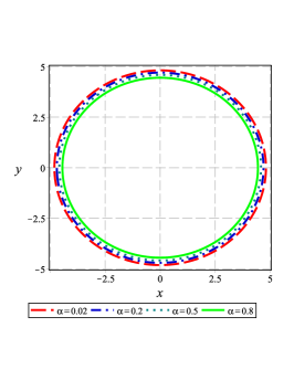
(b)  $Q=\beta=0.2$ and $\Lambda=-0.02$

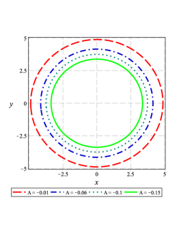
(c)  $\alpha=\beta=Q=0.2$

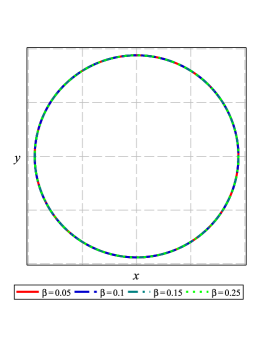
(d)  $Q=\alpha=0.2$ and $\Lambda=-0.02$

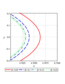
(e)  $Q=\alpha=0.2$ and $\Lambda=-0.02$

Figure 1: The plots depict the black hole shadow in the celestial plane $(x-y)$ for $M=1$. See the text for more details.

It has been known that the black hole shadow corresponds to its high energy absorption cross section for a distant observer. Indeed, the absorption cross section oscillates near to a limiting constant value $\sigma_{\rm lim}$ for a spherically symmetric black hole. According to WWei ; Belhaj1 ; Belhaj2 , $\sigma_{\rm lim}$ was found to be equal to the area of the photon sphere ($\sigma_{\rm lim}\approx\pi r_{s}^{2}$). Since the shadow measures the optical appearance of a black hole, it can be equal to the limiting constant value of the high-energy absorption cross section. The energy emission rate is given by

$$\frac{d^{2}E(\omega)}{dtd\omega}=\frac{2\pi^{3}\omega^{3}r_{s}^{2}}{e^{\frac{\omega}{T}}-1},$$ (17)

where $\omega$ and $T$ are, respectively, the emission frequency and Hawking temperature. For the present solution, the Hawking temperature is obtained as

$$T=\frac{1}{4\pi r_{e}}\left[\frac{-\Lambda r_{e}^{4}-3\alpha+2\beta^{2}r_{e}^{4}\left(1-\sqrt{1+\frac{Q^{2}}{\beta^{2}r_{e}^{4}}}\right)}{r_{e}^{2}+2\alpha}+1\right].$$ (18)

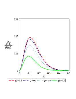
(a)  $\alpha=\beta=0.2$ and $\Lambda=-0.02$

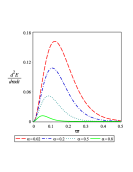
(b)  $Q=\beta=0.2$ and $\Lambda=-0.02$

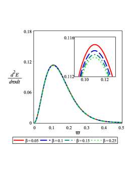
(c)  $Q=\alpha=0.2$ and $\Lambda=-0.02$

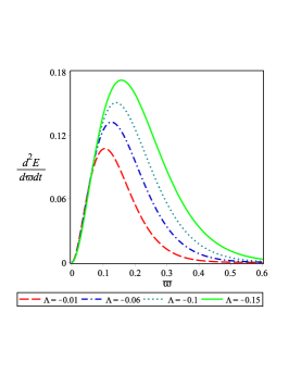
(d)  $\alpha=\beta=Q=0.2$

Figure 2: The energy emission rates for the corresponding black hole, with $M=1$, and different values of $Q$, $\beta$, $\alpha$ and $\Lambda$. See the text for for details.

Figure 2 depicts the behavior of the BH parameters on the energy emission. As it is transparent, there exists a peak of the energy emission rate for the black hole. As the BH parameters increase, the peak decreases and shifts to the low frequency. From Fig. 2(a), we verify that the electric charge decreases the energy emission, so that when the black hole is located in a more powerful electric field, the evaporation process would be slower. Regarding the effects of the GB and BI parameters, we see from Figs. 2(b) and 2(c), that increasing these two parameters results in the decrease of the energy emission. In fact, decreasing the coupling constants implies a fast emission of particles. But as in the shadow case, the effect of $\beta$ is negligible. Figure 2(d) displays the decreasing contribution of the cosmological constant on the emission rate which shows that the black hole should be located in a lower curvature background in order to have a faster evaporation. The figure also shows that the variation of cosmological constant has a stronger effect on the radiation rate than other parameters.

IV Connection between shadow radius and Quasinormal modes

Quasinormal modes (QNMs) are characteristic frequencies with a nonvanishing imaginary part, which encode important information related to the stability of the black hole under small perturbations. These frequencies depend on the details of the geometry and the type of the perturbation, but not on the initial conditions. To study these modes, an outgoing boundary condition should be imposed at infinity and an ingoing boundary condition at the horizon. In general, QNMs are characterized by complex numbers, $\omega=\omega_{R}+i\omega_{I}$. The sign of the imaginary part determines if the mode is stable or unstable. For positive $\omega_{I}$ (exponential growth), the mode is unstable, whereas negativity represents stable modes. In fact, it was shown that the real and imaginary parts of QNMs in the eikonal limit are, respectively, related to the angular velocity and Lyapunov exponent of unstable circular null geodesics QNM1 . It is worthwhile to mention that such a correspondence is only guaranteed for test fields, and not for gravitational ones QNM22 . Such a connection was investigated between QNMs and gravitational lensing QNM2 .

Recently, it has been suggested that the real part of QNMs in the eikonal limit can be connected to the radius of the black hole shadow QNM3 ; QNM4 . Such a correspondence has been applied to different black holes QNM5 ; QNM6 ; QNM7 . Here, we employ this idea and study the QNMs for the black hole solution presented by the metric function given in Eq. (8). According to this correspondence, the quasinormal frequency $\omega$ can be calculated with the property of the photon sphere as

$$\omega=l\Omega-i\left(n+\frac{1}{2}\right)|\lambda|.$$ (19)

where $n$ and $l$ are the overtone number and the multiple number (also called the angular quantum number), respectively. The quantities $\Omega$ and $\lambda$ are the angular velocity and Lyapunov exponent of the photon sphere, which can be obtained as

$$\Omega=\frac{\sqrt{f(r_{p})}}{r_{p}}=\frac{1}{L_{p}},$$ (20)

$$\lambda=\frac{\sqrt{2f(r_{p})-r_{p}^{2}f^{\prime\prime}}}{\sqrt{2}L_{p}}.$$ (21)

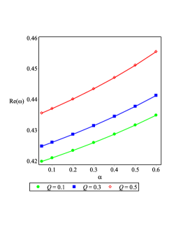
(a)  $\beta=0.2$ and $\Lambda=-0.02$

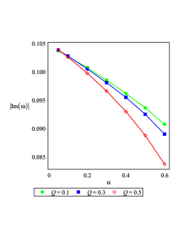
(b)  $\beta=0.2$ and $\Lambda=-0.02$

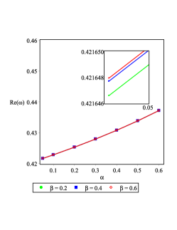
(c)  $Q=0.2$ and $\Lambda=-0.02$

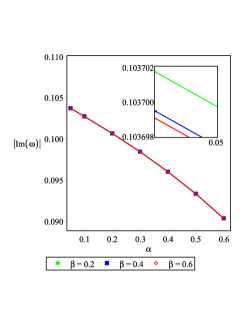
(d)  $Q=0.2$ and $\Lambda=-0.02$

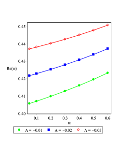
(e)  $Q=\beta=0.2$

(f)  $Q=\beta=0.2$

Figure 3: The behavior of $Re(\omega)$ and $Im(\omega)$ with respect to the GB parameter for $M=1$, $n=0$, $l=2$ and different values of $Q$ (Figs. 3(a) and 3(b)), $\beta$ (Figs. 3(c) and 3(d)) and $\Lambda$ (Figs. 3(e) and 3(f)). See the text for more details.

From Eq. (19), evidently the real part of the modes is proportional to the angular degree, whereas the imaginary part depends on the overtone number only. Using Eqs. (19), (20) and (21), we can investigate how the black hole parameters affect quasinormal frequencies. These effects are depicted in Fig. 3, where the spectrum obtained exhibits the following features:

• The real (imaginary) part of the quasinormal frequencies exhibits an increasing (decreasing) behavior for increasing $\alpha$. This shows that the scalar field perturbations around a black hole with a stronger GB coupling oscillates with more energy and decays slower.

• According to Figs. 3(a) and 3(b), the electric charge increases (decreases) the real (imaginary) value of the QNM frequency. This indicates that the scalar field perturbations in the presence of electric charge oscillate faster and decay slower as compared to neutral black holes.

• From Figs. 3(c) and 3(d), we verify that the effect of the BI parameter is similar to the GB parameter, but unlike the GB coupling constant, its effect is negligible.

• Both $Re(\omega)$ and $Im(\omega)$ decrease by increasing $\Lambda$, which is transparent from Figs. 3(e) and 3(f). This implies that the existence of a higher curvature background restrains the oscillation amplitude of the scalar field, even though it could decay slower.

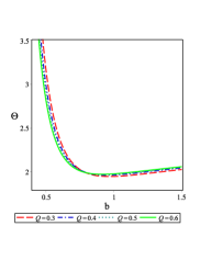
(a)  $\alpha=\beta=0.2$ and $\Lambda=-0.02$

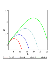
(b)  $\alpha=\beta=0.2$ and $\Lambda=-0.02$

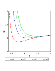
(c)  $Q=\beta=0.2$ and $\Lambda=-0.02$

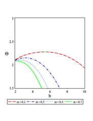
(d)  $Q=\beta=0.2$ and $\Lambda=-0.02$

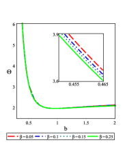
(e)  $Q=\alpha=0.2$ and $\Lambda=-0.02$

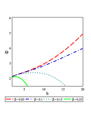
(f)  $Q=\alpha=0.2$ and $\Lambda=-0.02$

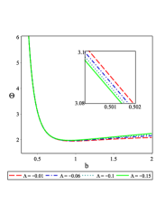
(g)  $\alpha=\beta=Q=0.2$

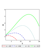
(h)  $\alpha=\beta=Q=0.2$

Figure 4: The behavior of $\Theta$ with respect to the impact parameter $b$ for $M=1$ and different values of $Q$, $\beta$, $\alpha$ and $\Lambda$. See the text for more details.

V Deflection angle using null geodesics

In this section, we study the light deflection around the black hole solution (8). Employing the null geodesics method Chandrasekhar ; Weinberg ; Kocherlakota ; WJaved , one can determine the total deflection $\Theta$ by the following relation

$$\Theta=2\int_{b}^{\infty}\Big{|}\frac{d\phi}{dr}\Big{|}dr-\pi,$$ (22)

where $b$ is the impact parameter, defined as $b\equiv L/E$. Using Eq. (22), the deflection angle is obtained as

$$\Theta = \frac{M\alpha(24Mb+7Q^{2})}{42b^{5}}+\frac{(2\alpha\Lambda-3)(2Q^{2}+15Mb)}{90b^{2}}$$

$$-\frac{2b^{2}\beta^{2}(2\alpha\Lambda-3)}{27}{~{}}_{2}F_{1}\left(-\frac{3}{4},-\frac{1}{2},\frac{5}{4},-\frac{Q^{2}}{\beta^{2}b^{4}}\right)$$

$$-\frac{2\alpha b^{2}\beta^{4}(5Q^{2}+24Mb)}{189Q^{2}}{~{}}_{2}F_{1}\left(-\frac{7}{4},-\frac{3}{2},-\frac{3}{4},-\frac{Q^{2}}{\beta^{2}b^{4}}\right)$$

$$+\frac{7}{3}+\frac{\Lambda b^{2}(\alpha\Lambda-3)}{9}+\frac{2\beta^{2}}{27b^{2}}\big{[}(2\alpha Q^{2}+12\alpha Mb$$

$$\qquad+b^{4}(2\alpha\Lambda-3)\big{]}{~{}}_{2}F_{1}\left(-\frac{3}{4},-\frac{1}{2},\frac{1}{4},-\frac{Q^{2}}{\beta^{2}b^{4}}\right).$$ (23)

Figure 4 depicts the impact of the black hole parameters on the deflection angle. More specifically, Figs. 4(a) and 4(b) illustrate the effect of electric charge on $\Theta$. One verifies that $\Theta$ is a decreasing (an increasing) function of $Q$ for small (large) values of the impact parameter. Figures 4(c) and 4(d) indicate the behavior of $\Theta$ by varying the GB parameter. As we see, for small values of $b$, the effect of $\alpha$ is to increase the deflection angle, whereas for large $b$, its effect is to decrease $\Theta$. This shows that the effect of $Q$ and $\alpha$ on the deflection angle is opposed to each other. Now, analysing Figs. 4(e) and 4(f), we verify that for all values of the impact parameter, increasing the BI parameter leads to the decreasing of $\Theta$. Regarding the cosmological constant effect, we see from Figs. 4(g) and 4(h), that its effect is similar to that of the GB parameter. Using Fig. 4, one can also analyze the behavior of $\Theta$ by varying the impact parameter. We verify that for small and large values of $b$, the deflection angle is a decreasing function of $b$, whereas for intermediate values, it is an increasing function; except for low values of $\beta$, where the increasing behavior is observed for large values of $b$ as well (see dashed line in Fig. 4(f)).

VI Summary and Conclusion

Motivated by interesting properties of black hole solutions in the recently proposed regularized 4D EGB theory of gravity, we considered Born-Infeld black holes and studied their dynamic features including the shadow size, energy emission rate, quasinormal modes and deflection angle. We first investigated the shadow behavior and photon sphere and examined how the black hole parameters affect them. The results showed that the GB parameter decrease both the photon sphere radius and shadow size, albeit, these quantities are not that sensitive to this parameter. Studying the effect of electric charge, we noticed that its effect was similar to that of GB coupling constant. However, the effect of the cosmological constant differs. Although it decreases the photon sphere radius, it has an increasing effect on the shadow size. Then, we performed an investigation regarding the energy emission rate and analyzed the effective roles of these parameters on this optical quantity. We found that all these parameters have a decreasing contribution on the emission rate, namely, the emission of particles around the black hole decreases by increasing these parameters. This revealed the fact that such black holes have a longer lifetime if they are located in a background with higher curvature or in a stronger electric field.

Furthermore, we employed the connection between the radius of the shadow and quasinormal modes and studied small perturbations around the black holes. We found that: i) As the coupling constants increase the real part (absolute value of the imaginary part) of the quasinormal frequencies increases (decreases). This means that QNMs oscillate faster and decay slower around the black holes with powerful coupling. ii) The effect of the cosmological constant is to decrease both real and imaginary parts of the QNMs. In other words, scalar perturbations have less energy for oscillation and decay slower in a higher curvature background. iii) The real (imaginary) part of QNM is an increasing (decreasing) function of the electric charge. In fact, the scalar field perturbations in the presence of electric charge oscillate faster and decay more slowly compared to neutral black holes.

Finally, we presented a study in the context of the gravitational lensing of light around these black holes. Depending on the choice of the BH parameters, we observed different behaviors. For small and large values of $b$, the deflection angle is a decreasing function of $b$, whereas for intermediate values, it is an increasing function. Relative to the impact of electric charge, we found that its effect is dependent on the values of the impact parameter, such that for small values of $b$, $\Theta$ is a decreasing function of $Q$, however, for large values, the effect of $Q$ is opposite. We also found that the effects of the GB parameter and the cosmological constant on the deflection angle are opposed to that of the electric charge. Regarding the influence of BI parameter, it had a decreasing effect for all values of $b$, although quite insignificant.

Here, we studied the optical features of the black hole solution in a modified gravity. There are other interesting solutions such as charged accelerating AdS black holes in $f(R)$ gravity Zhang:a , black bounce solutions Lobo and regular black holes with an asymptotically Minkowski core Berry:a which we are currently studying. The results will appear elsewhere.

- (1) D. Glavan and C. Lin, Einstein–Gauss–Bonnet Gravity in Four–Dimensional Spacetime, Phys. Rev. Lett. 124, 081301 (2020), [arXiv:1905.03601].
- (2) W. Ai, A note on the novel 4D Einstein–Gauss–Bonnet gravity, Commun. Theor. Phys. 72, 095402 (2020), [arXiv:2004.02858].
- (3) F. Shu, Vacua in novel 4D Einstein–Gauss–Bonnet Gravity: pathology and instability?, Phys. Lett. B 811, 135907 (2020), [arXiv:2004.09339].
- (4) M. Gurses, T. C. Sisman and B. Tekin, Is there a novel Einstein–Gauss–Bonnet theory in four dimensions?, Eur. Phys. J. C 80, 647 (2020), [arXiv:2004.03390].
- (5) S. Mahapatra, A note on the total action of 4D Gauss–Bonnet theory, Eur. Phys. J. C 80, 992 (2020), [arXiv:2004.09214].
- (6) R. A. Hennigar, D. Kubiznak, R. B. Mann and C. Pollack, On Taking the limit of Gauss–Bonnet Gravity: Theory and Solutions, JHEP 07, 027 (2020), [arXiv:2004.09472].
- (7) J. Arrechea, A. Delhom and A. Jiménez-Cano, Inconsistencies in four-dimensional Einstein-Gauss-Bonnet gravity, arXiv:2004.12998.
- (8) M. Gurses, T. C. Sisman and B. Tekin, Comment on “Einstein–Gauss–Bonnet Gravity in Four–Dimensional Space-Time”, Phys. Rev. Lett. 125, 149001 (2020), [arXiv:2009.13508].
- (9) J. Arrechea, A. Delhom and A. Jiménez-Cano, Comment on “Einstein–Gauss–Bonnet Gravity in Four–Dimensional Spacetime”, Phys. Rev. Lett. 125, 149002 (2020), [arXiv:2009.10715].
- (10) A. Casalino, A. Colleaux, M. Rinaldi and S. Vicentini, Regularized Lovelock gravity, arXiv:2003.07068.
- (11) H. Lu and Y. Pang, Horndeski Gravity as Limit of Gauss-Bonnet, Phys. Lett. B 809, 135717 (2020), [arXiv:2003.11552].
- (12) T. Kobayashi, Effective scalar-tensor description of regularized Lovelock gravity in four dimensions, JCAP 07, 013 (2020), [arXiv:2003.12771].
- (13) K. Aoki, M. A. Gorji and S. Mukohyama, A consistent theory of Einstein-Gauss-Bonnet gravity, Phys. Lett. B 810, 135843 (2020), [arXiv:2005.03859].
- (14) K. Aoki, M. A. Gorji and S. Mukohyama, Cosmology and gravitational waves in consistent Einstein-Gauss-Bonnet gravity, JCAP 2009, 014 (2020), [arXiv:2005.08428].
- (15) K. Aoki, M. A. Gorji, S. Mizuno and S. Mukohyama, Inflationary gravitational waves in consistent Einstein-Gauss-Bonnet gravity, arXiv:2010.03973.
- (16) P. G. S. Fernandes, Charged Black Holes in AdS Spaces in Einstein Gauss-Bonnet Gravity, Phys. Lett. B 805, 135468 (2020), [arXiv:2003.05491].
- (17) R. A. Konoplya and A. Zhidenko, Black holes in the four-dimensional Einstein-Lovelock gravity, Phys. Rev. D 101, 084038 (2020), [arXiv:2003.07788].
- (18) A. Kumar and R. Kumar, Bardeen black holes in the novel Einstein-Gauss-Bonnet gravity, arXiv:2003.13104.
- (19) A. Kumar and S. G. Ghosh, Hayward black holes in the novel Einstein-Gauss-Bonnet gravity, arXiv:2004.01131.
- (20) Y. P. Zhang, S. W. Wei and Y. X. Liu, Spinning test particle in four-dimensional Einstein-Gauss-Bonnet Black Hole, Universe 6, 103 (2020), [arXiv:2003.10960].
- (21) S. Shaymatov, J. Vrba, D. Malafarina, B. Ahmedov and Z. Stuchlík, Charged particle and epicyclic motions around Einstein–Gauss–Bonnet black hole immersed in an external magnetic field, Phys. Dark Univ. 30, 100648 (2020), [arXiv:2005.12410].
- (22) R. A. Konoplya and A. F. Zinhailo, Quasinormal modes, stability and shadows of a black hole in the novel 4D Einstein-Gauss-Bonnet gravity, Eur. Phys. J. C 80, 1049 (2020), [arXiv:2003.01188].
- (23) M. Guo and P. C. Li, Innermost stable circular orbit and shadow of the Einstein–Gauss–Bonnet black hole, Eur. Phys. J. C 80, 588 (2020), [arXiv:2003.02523].
- (24) B. Eslam Panah, K. Jafarzade and S. H. Hendi, Charged 4D Einstein-Gauss-Bonnet-AdS Black Holes: Shadow, Energy Emission, Deflection Angle and Heat Engine, Nucl. Phys. B 961, 115269 (2020), [arXiv:2004.04058].
- (25) X. X. Zeng, H. Q. Zhang and H. Zhang, Shadows and photon spheres with spherical accretions in the four-dimensional Gauss-Bonnet black hole, Eur. Phys. J. C 80, 872 (2020), [arXiv:2004.12074].
- (26) K. Hegde, A. Naveena Kumara, C. L. A. Rizwan, A. K. M. and M. S. Ali, Thermodynamics, Phase Transition and Joule Thomson Expansion of novel 4-D Gauss Bonnet AdS Black Hole, arXiv:2003.08778.
- (27) D. V. Singh and S. Siwach, Thermodynamics and P-v criticality of Bardeen-AdS Black Hole in 4 Einstein-Gauss-Bonnet Gravity, Phys. Lett. B 808, 135658 (2020), [arXiv:2003.11754].
- (28) R. Kumar and S. G. Ghosh, Rotating black holes in Einstein-Gauss-Bonnet gravity and its shadow, JCAP 07, 053 (2020), [arXiv:2003.08927].
- (29) S. W. Wei and Y. X. Liu, Testing the nature of Gauss-Bonnet gravity by four-dimensional rotating black hole shadow, arXiv:2003.07769.
- (30) R. A. Konoplya and A. Zhidenko, Simply rotating higher dimensional black holes in Einstein-Gauss-Bonnet theory, Phys. Rev. D 102, 084030 (2020), [arXiv:2007.10116].
- (31) S. G. Ghosh and S. D. Maharaj, Radiating black holes in the novel 4D Einstein-Gauss-Bonnet gravity, Phys. Dark Univ. 30, 100687 (2020), [arXiv:2003.09841].
- (32) R. A. Konoplya and A. Zhidenko, (In)stability of black holes in the 4D Einstein-Gauss-Bonnet and Einstein-Lovelock gravities, Phys. Dark Univ. 30, 100697 (2020), [arXiv:2003.12492].
- (33) S. A. Hosseini Mansoori, Thermodynamic geometry of the novel 4-D Gauss Bonnet AdS Black Hole, arXiv:2003.13382.
- (34) S. W. Wei and Y. X. Liu, Extended thermodynamics and microstructures of four-dimensional charged Gauss-Bonnet black hole in AdS space, Phys. Rev. D 101, 104018 (2020), [arXiv:2003.14275].
- (35) R. A. Konoplya and A. F. Zinhailo, Grey-body factors and Hawking radiation of black holes in Einstein-Gauss-Bonnet gravity, Phys. Lett. B 810, 135793 (2020), [arXiv:2004.02248].
- (36) C. Y. Zhang, S. J. Zhang, P. C. Li and M. Guo, Superradiance and stability of the regularized 4D charged Einstein-Gauss-Bonnet black hole, JHEP 08, 105 (2020), [arXiv:2004.03141].
- (37) A. Aragón, R. Bécar, P. A. González and Y. Vásquez, Perturbative and nonperturbative quasinormal modes of 4D Einstein–Gauss–Bonnet black holes, Eur. Phys. J. C 80, 773 (2020), [arXiv:2004.05632].
- (38) P. Liu, C. Niu and C. Y. Zhang, Instability of the novel 4D charged Einstein-Gauss-Bonnet de-Sitter black hole, arXiv:2004.10620.
- (39) S. U. Islam, R. Kumar and S. G. Ghosh, Gravitational lensing by black holes in the Einstein-Gauss-Bonnet gravity, JCAP 09, 030 (2020), [arXiv:2004.01038].
- (40) C. Liu, T. Zhu and Q. Wu, Thin Accretion Disk around a four-dimensional Einstein-Gauss-Bonnet Black Hole, arXiv:2004.01662.
- (41) X. H. Ge and S. J. Sin, Causality of black holes in 4-dimensional Einstein–Gauss–Bonnet–Maxwell theory, Eur. Phys. J. C 80, 695 (2020), [arXiv:2004.12191].
- (42) N. Dadhich, On causal structure of -Einstein–Gauss–Bonnet black hole, Eur. Phys. J. C 80, 832 (2020), [arXiv:2005.05757 ].
- (43) D. V. Singh, R. Kumar, S. G. Ghosh and S. D. Maharaj, Phase transition of AdS black holes in 4D EGB gravity coupled to nonlinear electrodynamics, Ann. Phys. 424, 168347 (2021), [arXiv:2006.00594].
- (44) S. G. Ghosh, D. V. Singh and S. D. Maharaj, Regular black holes in Einstein-Gauss-Bonnet gravity, Phys. Rev. D 97, 104050 (2018).
- (45) K. Jafarzade, M. Kord Zangeneh and F. S. N. Lobo, Optical features of AdS black holes in the novel 4D Einstein-Gauss-Bonnet gravity coupled to nonlinear electrodynamics, arXiv:2009.12988.
- (46) K. Yang, B. M. Gu, S. W. Wei and Y. X. Liu, Born–Infeld black holes in 4D Einstein–Gauss–Bonnet gravity, Eur. Phys. J. C 80, 662 (2020), [arXiv:2004.14468].
- (47) K. Jusufi, Nonlinear magnetically charged black holes in 4D Einstein-Gauss-Bonnet gravity, Annals Phys. 421, 168285 (2020), [arXiv:2005.00360].
- (48) K. Akiyama et al., First M87 Event Horizon Telescope Results. I. The Shadow of the Supermassive Black Hole, Astrophys. J. 875, L1 (2019), [arXiv:1906.11238].
- (49) K. Akiyama et al, First M87 Event Horizon Telescope Results. IV. Imaging the Central Supermassive Black Hole, Astrophys. J. 875, L4 (2019), [arXiv:1906.11241].
- (50) M. Born and L. Infeld, Foundations of the new field theory, Proc. R. Soc. Lond. A 144, 425 (1934).
- (51) E. S. Fradkin and A. A. Tseytlin, Effective field theory from quantized string, Phys. Lett. B 163, 123 (1985).
- (52) R. R. Metsaev, M. A. Rakhmanov and A. A. Tseytlin, The Born-Infeld action as the effective action in the open superstring theory, Phys. Lett. B 193, 207 (1987).
- (53) E. Bergshoeff, E. Sezgin, C. Pope and P. Townsend, The Born-lnfeld action from conformal invariance of the open superstring, Phys. Lett. B 188, 70 (1987).
- (54) D. L. Burke et al., Positron Production in Multiphoton Light-by-Light Scattering, Phys. Rev. Lett. 79, 1626 (1997).
- (55) C. Bamber et al., Studies of nonlinear QED in collisions of 46.6-GeV electrons with intense laser pulses, Phys. Rev. D 60, 092004 (1999).
- (56) D. Tommasini, A. Ferrando, H. Michinel and M. Seco, Detecting photon-photon scattering in vacuum at exawatt lasers, Phys. Rev. A 77, 042101 (2008), [arXiv:0802.0101].
- (57) D. Tommasini, A. Ferrando, H. Michinel and M. Seco, Precision tests of QED and non-standard models by searching photon-photon scattering in vacuum with high power lasers, J. High Energy Phys. 0911, 043 (2009), [arXiv:0909.4663].
- (58) O. J. Pike, F. Mackenroth, E. G. Hill and S. J. Rose, A photon–photon collider in a vacuum hohlraum, Nature Photonics 8, 434 (2014).
- (59) P. Vargas Moniz, Quintessence and Born-Infeld cosmology, Phys. Rev. D 66, 103501 (2002).
- (60) D. N. Vollick, Homogeneous and isotropic cosmologies with nonlinear electromagnetic radiation, Phys. Rev. D 78, 063524 (2008), [arXiv:0807.0448].
- (61) C. Corda and H. J. Mosquera Cuesta, Inflation from gravity: a new approach using nonlinear electrodynamics, Astropart. Phys.34, 587 (2011), [ arXiv:1011.4801].
- (62) V. A. De Lorenci, R. Klippert, M. Novello and J. M. Salim, Nonlinear electrodynamics and FRW cosmology Phys. Rev.D 65, 063501 (2002), [arXiv:gr-qc/9806076].
- (63) C. Corda and H. J. Mosquera Cuesta, Removing black-hole singularities with nonlinear electrodynamics, Mod. Phys. Lett. A 25, 2423 (2010), [arXiv:0905.3298].
- (64) A. Allahyari, M. Khodadi, S. Vagnozzi and D. F. Mota, Magnetically charged black holes from non-linear electrodynamics and the Event Horizon Telescope, JCAP 02, 003 (2020), [arXiv:1912.08231].
- (65) Y. M. Xu, H. M. Wang, Y. X. Liu and S. W. Wei, Photon sphere and reentrant phase transition of charged Born-Infeld-AdS black holes, Phys. Rev. D 100, 104044 (2019), [arXiv:1906.03334].
- (66) A. S. Habibina and H. S. Ramadhan, Geodesic of nonlinear electrodynamics and stable photon orbits, Phys. Rev. D 101, 124036 (2020), [arXiv:2007.03211].
- (67) H. J. Mosquera Cuesta and J. M. Salim, Non-linear electrodynamics and the gravitational redshift of highly magnetized neutron stars, Mon. Not. Roy. Astron. Soc. 354, L55 (2004), [arXiv:astro-ph/0403045].
- (68) H. J. Mosquera Cuesta and J. M. Salim, Nonlinear electrodynamics and the surface redshift of pulsars, Astrophys. J. 608, 925 (2004), [arXiv:astro-ph/0307513].
- (69) Z. Bialynicka-Birula and I. Bialynicka-Birula, Nonlinear Effects in Quantum Electrodynamics. Photon Propagation and Photon Splitting in an External Field, Phys. Rev. D 2, 2341 (1970).
- (70) M. Aiello, R. Ferraro and G. Giribet, Exact solutions of Lovelock-Born-Infeld black holes, Phys. Rev. D 70, 104014 (2004), [arXiv:gr-qc/0408078].
- (71) D. Zou, Z. Yang, R. Yue and P. Li, Thermodynamics of Gauss-Bonnet-Born-Infeld black holes in AdS space, Mod. Phys. Lett. A 26, 515 (2011), [arXiv:1011.3184].
- (72) V. Perlick, O.Y. Tsupko and G.S. Bisnovatyi-Kogan, Influence of a plasma on the shadow of a spherically symmetric black hole, Phys. Rev. D 92, 104031 (2015), [arXiv:1507.04217].
- (73) S. W. Wei and Y. X. Liu, Observing the shadow of Einstein–Maxwell–Dilaton–Axion black hole, JCAP 11, 063 (2013), [arXiv:1311.4251].
- (74) A. Belhaj, M. Benali, A. El Balali, H. El Moumni and S. E. Ennadifi, Deflection Angle and Shadow Behaviors of Quintessential Black Holes in arbitrary Dimensions, Class. Quant. Grav. 37, 215004 (2020), [arXiv:2006.01078].
- (75) A. Belhaj, M. Benali, A. El Balali, W. El Hadri and H. El Moumni, Shadows of Charged and Rotating Black Holes with a Cosmological Constant, arXiv:2007.09058.
- (76) V. Cardoso, A. S. Miranda, E. Berti, H. Witek and V. T. Zanchin, Geodesic stability, Lyapunov exponents, and quasinormal modes, Phys. Rev. D 79, 064016 (2009), [arXiv:0812.1806].
- (77) R. A. Konoplya, Z. Stuchlik, Are eikonal quasinormal modes linked to the unstable circular null geodesics? Phys. Lett. B 771, 597 (2017), [arXiv:1705.05928].
- (78) I. Z. Stefanov, S. S. Yazadjiev and G. G. Gyulchev, Connection between black-hole quasinormal modes and lensing in the strong deflection limit, Phys. Rev. Lett. 104, 251103 (2010), [arXiv:1003.1609].
- (79) K. Jusufi, Quasinormal Modes of Black Holes Surrounded by Dark Matter and Their Connection with the Shadow Radius, Phys. Rev. D 101, 084055 (2020), [arXiv:1912.13320].
- (80) K. Jusufi, Connection Between the Shadow Radius and Quasinormal Modes in Rotating Spacetimes, Phys. Rev. D 101, 124063 (2020), [arXiv:2004.04664].
- (81) Y. Guo and Y. G. Miao, Null geodesics, quasinormal modes and the correspondence with shadows in high-dimensional Einstein-Yang-Mills spacetimes, Phys. Rev. D 102, 084057 (2020), [arXiv:2007.08227].
- (82) C. Lan, Y. G. Miao and H. Yang, Quasinormal Modes and Thermodynamics of Regular Black Holes, arXiv:2008.04609.
- (83) S. W. Wei and Y. X. Liu, Null geodesics, Quasinormal modes, and thermodynamic phase transition for charged black holes in asymptotically flat and dS spacetimes, Chin .Phys. C 44, 115103 (2020), [arXiv:1909.11911].
- (84) S. Chandrasekhar, The Mathematical Theory of Black Holes, Oxford University Press, New York (1983).
- (85) S. Weinberg, Gravitation and Cosmology: Principles and Applications of the General Theory of Relativity, Wiley, New York (1972).
- (86) P. Kocherlakota and L. Rezzolla, Accurate mapping of spherically symmetric black holes in a parameterised framework, Phys. Rev. D 102, 064058 (2020), [arXiv:2007.15593].
- (87) W. Javed, J. Abbas and A. Övgün, Effect of the quintessential dark energy on weak deflection angle by Kerr-Newmann Black hole, Ann. Phys. 418, 168183 (2020), [arXiv:2007.16027].
- (88) M. Zhang and R. B. Mann, Charged accelerating black hole in f(R) gravity, Phys. Rev. D 100, 084061 (2019), [arXiv:1908.05118].
- (89) F. S. N. Lobo, A. Simpson and M. Visser, Dynamic thin-shell black-bounce traversable wormholes, Phys. Rev. D 101, 124035 (2020), [arXiv:2003.09419].
- (90) T. Berry, F. S. N. Lobo, A. Simpson and M. Visser, Thin-shell traversable wormhole crafted from a regular black hole with asymptotically Minkowski core, Phys. Rev. D 102, 064054 (2020), [arXiv:2008.07046].