DynamiTe: Dynamic Termination and Non-Termination Proofs

Abstract.

There is growing interest in termination reasoning for non-linear programs and, meanwhile, recent dynamic strategies have shown they are able to infer invariants for such challenging programs. These advances led us to hypothesize that perhaps such dynamic strategies for non-linear invariants could be adapted to learn recurrent sets (for non-termination) and/or ranking functions (for termination).

In this paper, we exploit dynamic analysis and draw termination and non-termination as well as static and dynamic strategies closer together in order to tackle non-linear programs. For termination, our algorithm infers ranking functions from concrete transitive closures, and, for non-termination, the algorithm iteratively collects executions and dynamically learns conditions to refine recurrent sets. Finally, we describe an integrated algorithm that allows these algorithms to mutually inform each other, taking counterexamples from a failed validation in one endeavor and crossing both the static/dynamic and termination/non-termination lines, to create new execution samples for the other one.

We have implemented these algorithms in a new tool called DynamiTe. For non-linear programs, there are currently no SV-COMP termination benchmarks so we created new sets of 38 terminating and 39 non-terminating programs. Our empirical evaluation shows that we can effectively guess (and sometimes even validate) ranking functions and recurrent sets for programs with non-linear behaviors. Furthermore, we show that counterexamples from one failed validation can be used to generate executions for a dynamic analysis of the opposite property. Although we are focused on non-linear programs, as a point of comparison, we compare DynamiTe’s performance on linear programs with that of the state-of-the-art tool, Ultimate. Although DynamiTe is an order of magnitude slower it is nonetheless somewhat competitive and sometimes finds ranking functions where Ultimate was unable to. Ultimate cannot, however, handle the non-linear programs in our new benchmark suite.

Supplemental Materials. Our materials are available at https://github.com/letonchanh/dynamite.

1. Introduction

Termination continues to be an important theoretical property that is of practical interest. In recent years, there has been a proliferation of termination and non-termination verification tools, including T2 (Brockschmidt, 2020), Ultimate (Ultimate, 2020), CPAchecker (Beyer and Keremoglu, 2011), AProVE (Giesl et al., 2014), FuncTion (Urban, 2015), SeaHorn (Gurfinkel et al., 2015), HipTNT+ (Le et al., 2015), and many others (see the Termination track of SV-COMP (Beyer, 2020)). These tools are very effective at proving termination and non-termination, especially for programs with linear arithmetic assignments and loop guards (Podelski and Rybalchenko, 2004a).

Meanwhile, researchers are increasingly using techniques based on dynamic execution, to bolster static verification. Static analysis explores all possible program paths but typically has one or more shortcomings: expressivity sacrifices, false positives, simpler invariants or restrictions on kinds of target programs. Dynamic analysis focuses on exploring only a few program executions and, as such, also has its own shortcomings: it is only correct with respect to the explored paths. However, by (initially) sacrificing soundness, dynamic analyses support more expressive invariants and scale well to large and complex programs (see, e.g., (O’Hearn, 2020)), often being effective even when the source code is not available. Moreover, false positives for the existence of a bug are not a concern: if any of the explored paths leads to an error, then it is a real error. More recent dynamic analyses have taken a “data-driven” or machine learning approach, i.e., learning based on training data. DIG (Nguyen et al., 2014a) and  (Yao et al., 2020) use this form of dynamic analysis to learn invariants of non-linear programs. Moreover, other recent works combine both dynamic and static analysis techniques in an iterative loop, sometimes for the purpose of termination reasoning (Nori and Sharma, 2013). The dynamic analysis component is used to “guess” some candidate results and the static analysis one is used to verify them. The results of the checker, e.g., counterexamples showing invalidity of the candidate results, are then used to help the dynamic analysis to infer better results.

Landscape. In the context of these recent advances that use dynamic support to learn invariants of non-linear programs, a natural question is whether they can be used or adapted to empower termination and non-termination reasoning for such challenging programs. We explored in this direction, asking first whether non-termination reasoning can be built from dynamic approaches for non-linear invariants, and then a similar question for termination. While these endeavors at first seem independent and could potentially be parallelized, we finally explored smarter approaches, where counterexamples from a failed termination proof could be used to generate executions for dynamically learning non-termination, and vice-versa.

Learning ranking functions and recurrent sets. In this paper, we present algorithms that mix static and dynamic strategies in order to prove termination and non-termination of non-linear programs. Overall, our strategy begins by sampling terminating and potentially non-terminating executions from an instrumented program, with truncated divergence. We first present a novel termination algorithm ProveT, which dynamically samples concrete states from the transitive closure of the loop bodies of sampled traces, fits them to a ranking function template, and uses an SMT solver to generate unknown coefficients in the template. We then attempt to validate these candidate ranking functions (via reachability) and use any possible counterexamples to dynamically generate more sample traces. A second ProveNT algorithm is used for non-termination, and iteratively refines a recurrent set condition, by executing the program and using samples to learn conditions for re-entering versus exiting the loop. We next widen the interfaces of these procedures and show that these algorithms can inform each other. A failed attempt of ProveT to prove termination yields a potentially infinite path, which we use to generate new executions to input to ProveNT, and vice-versa.

We have implemented these algorithms in a new tool called DynamiTe for dynamically proving termination and non-termination. DynamiTe employs the power of many disparate tools: the dynamic analysis tool DIG (Nguyen et al., 2014a), the symbolic execution tool CIVL (Siegel et al., 2015), the reachability analysis tools CPAchecker (Beyer and Keremoglu, 2011) and Ultimate (Ultimate, 2020) (without termination reasoning), and the SMT solvers Z3 (de Moura and Bjørner, 2008) and CVC4 (Barrett et al., 2011).

Our main goal is to prove termination and non-termination of non-linear programs, a domain for which many existing tools struggle. We evaluate DynamiTe on two existing benchmarks consisting of non-linear programs (polyrank (Bradley et al., 2005b), which has non-deterministic terminating programs, and Anant (Cook et al., 2014), which has non-linear non-terminating programs) and also create and evaluate DynamiTe on more challenging non-linear terminating and non-terminating benchmarks (by adapting the SV-COMP benchmark nla-digbench (2020) consisting of programs having nonlinear polynomial invariants). We show that DynamiTe is able to learn rich ranking functions and recurrent sets for these programs that cannot be handled by tools like Ultimate. We also show that the integrated algorithm can choose the right algorithm, ProveT or ProveNT  or use the counterexample from a failed proof to assist the other.

Although non-linear programs were our focus, we also compared our algorithms on linear programs against a state-of-the-art termination prover: Ultimate (Ultimate, 2020). We used the 62 benchmarks from the category termination-crafted-lit in SV-COMP 2020 and show that, although DynamiTe is typically an order of magnitude slower (owing to the need for program execution), it is nonetheless competitive with Ultimate, which is a much more mature tool. Also, in some cases DynamiTe is faster than Ultimate and in other cases DynamiTe is able to learn ranking functions, where Ultimate is unable to do so.

Contributions

In summary, we present:

1. A novel termination algorithm, based on sampling concrete states from the transitive closure and fitting to ranking function templates with SMT. (Section 4)

2. A novel non-termination algorithm, based on refining recurrent sets with conditions learned from dynamic executions of the program (Section 5).

3. An integrated algorithm for termination and non-termination, that uses counterexamples from one failed static validation attempt to generate executions for dynamic analysis of the other. (Section 6)

4. A new publicly available tool called DynamiTe (2020) for termination/non-termination of non-linear programs. (Section 7)

5. Two new benchmark suites for SV-COMP: one for termination of non-linear programs, and one for non-termination of non-linear programs. (Section 8)

6. An experimental evaluation, demonstrating that DynamiTe is able to learn and sometimes validate ranking functions and recurrent sets for non-linear programs. (Section 8)

Related work.

Similarly to DynamiTe, several existing works support programs with non-linear properties. Nori and Sharma (2013) show program termination by dynamically inferring (nonlinear, disjunctive) loop bounds from program execution traces. Bradley et al. (2005b, c) use finite difference trees to statically infer lexicographic polynomial ranking functions to prove termination of non-linear programs. For non-termination analysis,  Cook et al. (2014) uses abstract interpretation to over-approximate the non-linear programs and infer linear recurrent sets to prove program termination. Frohn and Giesl (2019) uses recurrence solvers to generate loop-free transitions so that paths to non-terminating loops can be discovered. In contrast, DynamiTe integrates existing dynamic invariant generation and static verification for dynamically analyze both program termination and non-termination from their concrete snapshots, and it can analyze many other programs that are not by these works (details in Sections 8 and 9). Also, DynamiTe can analyze termination properties for non-deterministic programs (similarly to (Nori and Sharma, 2013; Bradley et al., 2005b, c), but it currently cannot handle non-termination for non-deterministic programs (see Sections 3,  5 and 8.3 for additional discussion and evaluation). In Section 9 we discuss these works and other general termination and non-termination techniques in more details.

2. Overview

⬇

int a = 0, n = *;

while ((a+1) * (a+1) <= n):

a = a + 1

Consider the program to the right. In the loop body of this program, a is incremented by 1, and the loop terminates when the square of a+1 is no longer below n. While the termination of this program is intuitively obvious, existing tools (e.g. Ultimate, AProVE, SeaHorn) are unable to prove it to be terminating because it requires reasoning about the non-linear behavior of program variables. Proving termination here involves discovering a ranking function that pertains to variables occurring in a quadratic inequality in the loop condition. As we discuss below, examples like this and more complicated ones with polynomial expressions, foil many existing techniques that are based on linear arithmetic constraints. One major impediment appears to be the lack of static reasoning techniques for programs with such non-linear behaviors. Some static works have shown static termination reasoning for certain classes of non-linear programs (e.g. “NAW loops” (Babić et al., 2007), loops with finite difference trees (Bradley et al., 2005b, c)), and other works provide static resource bounds (Hoffmann and Hofmann, 2010b, a; Hoffmann et al., 2011; Gulwani, 2009; Gulwani et al., 2009), but still lack general techniques for termination and non-termination of these challenging programs.

Meanwhile, in recent years, a number of works have showed that dynamic analysis can be used to learn rich, non-linear invariants. Nguyen et al. (2012) showed that we can use dynamic analysis to learn expressive (non-linear) polynomial invariants from a small set of program execution traces. Subsequent works (Nguyen et al., 2017a, b) propose iterative loop algorithms to generate candidate invariants from traces and use symbolic execution to refute spurious results and generate valid counterexamples, which are then used to improve the invariant generation process. Many other works, e.g., (Sharma et al., 2013; Nguyen et al., 2014b), combine inferring non-linear invariants with static checking. Recently, Yao et al. (2020) proposes using neural networks to learn non-linear invariants.

2.1. Learning ranking functions and recurrent sets

In this paper, we explore the question of whether techniques for non-linear invariants can be extended to reasoning about both termination and non-termination and do so in an integrated way. We begin by adapting earlier dynamic analysis works, to provide a new route for learning ranking functions and recurrent sets. To highlight and illustrate the key features of our work, we will use the following pair of slightly more complicated examples. The following two programs are similar, but one terminates and the other does not:

Termination		Non-Termination
⬇ 1int s = 1, t = 1, k, c = 1 2while (t*t - 4*s + 2*t + 1 + c <= k): 3 t = t + 2 4 s = s + t 5 c = c + t\end{lstlisting} 6\end{minipage} 7&\hspace{0.14in}& 8\hspace{0.2in}\begin{minipage}{0.42\textwidth} 9% >>>>>>> 99075a21c66e3b3574a83cf06c4259eea45fe2a1 10\begin{lstlisting}[language=Python] 11int s = 1, t = 1, c = 1 12while (t*t - 4*s + 2*t + 1 + c >= 0): 13 t = t + 2 14 s = s + t 15 c = c + t

These examples are based on sqrt1.c from the SV-COMP benchmark nla-digbench (2020). (We discuss how we adapted it in Section 8.) Both of these programs involve loop conditions that are non-linear, given the quadratic term t*t in them. For illustration purposes, the body of both programs is the same, and it is not difficult to see by induction that the subexpression t*t - 4*s + 2*t + 1 in both loop conditions is always equal to 0.

In the program on the left, the loop condition is essentially equivalent to c <= k for all reachable states in the program. Given that k is initialized to a nondeterministic value and unchanged and t is always positive, and thus c is always increasing up to k and the execution will eventually exit the loop. This reasoning is usually captured with ranking functions: a map from every state to an ordered element where a transition in the program between states implies a transition from an element to a strictly smaller in that order element. Moreover, such an order is chosen to not be forever decreasing, and thus there cannot be an infinite sequence of states with valid program transitions between them. In this case such a function would be the one that maps every state to the value of k-c. It is the aim of our algorithm to synthesize this function and we describe in the following paragraphs how this is achieved.

In the program on the right, the loop condition is now essentially c >= 0 for all reachable states of the program, which holds trivially since c is initialized to 1 and always increasing. To show non-termination, a recurrent set is usually constructed: by abstracting the loop body in a relation $\mathcal{T}_{\texttt{loop}}$, a set $X$ of states is collected such that for any state $s$ in that set, and any other state $s^{\prime}$ we can transition to from $s$, it is the case that $s^{\prime}$ is also in $X$. The existence of such a set that contains reachable states implies that the program is non-terminating at least in some cases.

The above examples reiterate the point that, even for simple nonlinear programs, the necessary reasoning evades existing termination and non-termination tools, many of which are based on linear arithmetic constraint solving (Podelski and Rybalchenko, 2004a; Gurfinkel et al., 2015).

Dynamic snapshots for termination/non-termination.

In this paper, we work in a direction that is based on learning from dynamically generated program traces, for guessing (and possibly validating) ranking functions and recurrent sets for examples such as those above. To this end, we begin by describing a simple mechanism for collecting traces which may or may not terminate. Tools for dynamic analysis typically take “snapshots” of the state of the program to record trace information. These snapshots may record the values of some/all variables, as well as the program location and there are many techniques for injecting snapshots.

In the case of termination, though, there is the additional challenge of recording snapshots of a loop that may run forever. Our solution is to break the loop so that potentially infinite executions are truncated, and then we can learn about those prefixes and try to characterize the ones that would have terminated versus those that would not have. We can truncate loops by introducing a counter. Counter instrumentation is common in other kinds of static analysis (Gulwani, 2009; Gulwani et al., 2009; Hoffmann and Hofmann, 2010b, a; Hoffmann et al., 2011), but here we use it to truncate executions.

⬇

1int s = 1, t = 1, c = 1

2lightgrayint _ctr = 0, _bnd = 500

3lightgray${\bf vtrace}_{\texttt{pre}}$(s,t,c)

4while (t*t - 4*s + 2*t + 1 + c >= 0):

5 lightgrayif (_ctr > _bnd) abort() else _ctr++

6 lightgray${\bf vtrace}_{\texttt{body}}$(s,t,c)

7 t = t + 2

8 s = s + t

9 c = c + t

10lightgray${\bf vtrace}_{\texttt{post}}$(s,t,c)

Using the above non-termination example, our transformation generates the program on the right, where changes are indicated in the gray boxed regions. Technically, these changes are made to every loop of the program, but for illustrative purposes in the section we will just use one loop. Our transformation begins by introducing a pair of variables for the loop. The variable _ctr is used to count the loop’s iterations, and _bnd is an input to the dynamic analysis, whose value is pragmatically chosen to determine a useful prefix of potentially non-terminating traces. As such, _ctr is incremented inside the loop body and when it reaches _bnd, control exits the loop if it hasn’t already. Next, we inject function calls to a method ${\bf vtrace}$ in three places: before (${\bf vtrace}_{\texttt{pre}}$), during (${\bf vtrace}_{\texttt{body}}$), and after (${\bf vtrace}_{\texttt{post}}$) the loop. In each location, ${\bf vtrace}$ is used to record the values of the variables in scope as a tuple such as $(\texttt{\small body},\texttt{\small s}=1,\texttt{\small t}=1,\texttt{\small c}=1)$, which we call a “snapshot”. It should be noted that ${\bf vtrace}_{\texttt{post}}$ only captures values for states that exited the loop due to natural causes.

This truncation and instrumentation permits us to distinguish between three classes of traces:

$$\begin{array}[]{ccc}\bar{\pi}_{\texttt{base}}=\{(\texttt{\small pre},\_)\!\cdot\!(\texttt{\small post},\_)\},&\bar{\pi}_{\texttt{term}}=\{(\texttt{\small pre},\_)\!\cdot\!(\texttt{\small body},\_)^{+}\!\cdot\!(\texttt{\small post},\_)\},&\bar{\pi}_{\texttt{mayloop}}=\{(\texttt{\small pre},\_)\!\cdot\!(\texttt{\small body},\_)^{+}\}\\ \end{array}$$

Above we have described the classes of traces using simple regular expressions, matching the first component of the tuple, and ignoring the values of variables. Technically, by these expressions, we mean the set of all traces that match the regular expression. The first set of traces $\bar{\pi}_{\texttt{base}}$ are those that have a snapshot before the loop, skip the loop entirely and then have a snapshot immediately after the loop. The second set $\bar{\pi}_{\texttt{term}}$ is similar but has at least one snapshot from inside the body of the loop. The third set $\bar{\pi}_{\texttt{mayloop}}$ includes traces that entered the loop but for which there is no post-loop snapshot. (Of course the union of these languages covers the language of the program.) This transformation is unsound because (i) it does not account for loop body states beyond _bnd, and (ii) executions may be forced to exit the loop before their day has come to do so. However, as we will see, this strategy collects rich data that enables us to start making guesses for ranking functions and recurrent sets, even in non-linear contexts such as this example.

2.2. Algorithms

Learning ranking functions for termination.

In Section 4, we present an algorithm beginning with:

1. Instrumenting the program as discussed above.

2. Generating random inputs to the program and collect traces (as in (Nguyen et al., 2012, 2014a)).

3. Partitioning traces into $(\bar{\pi}_{\texttt{base}},\bar{\pi}_{\texttt{term}},\bar{\pi}_{\texttt{mayloop}})$.

4. Using $\bar{\pi}_{\texttt{term}}$ as an input to subprocedure InferRF$(\bar{\pi}_{\texttt{term}})$, discussed below, to infer a ranking function from the data.

For the above Termination example, such a possible trace is: $\{(\texttt{\small pre},1,1,42,1),(\texttt{\small body},1,1,42,1),$ $(\texttt{\small body},4,3,42,4),(\texttt{\small body},9,5,42,9),\ldots\}\in\bar{\pi}_{\texttt{term}}$, where each tuple represents variables (_,s,t,k,c). Running DynamiTe on this example takes 7.55 seconds to produce an answer. By comparison, existing tools for termination (Ultimate, 2020; CPAChecker, 2020; Gurfinkel et al., 2015; AProVE, 2020) typically perform well on linear programs, but fail to produce an answer on this program. The output of InferRF is the ranking function expression k-c. In some cases this guess may already be useful, even though it has not been verified. A user may wish to examine it and, in this case, it appears to be correct. If a stronger guarantee is needed, this ranking function can be given to a safety reachability prover such as (the reachability analyses of) CPAchecker (CPAChecker, 2020) or Ultimate (Ultimate, 2020). For example, using a standard translation (Cook et al., 2006), we can use an encoding that reduces ranking function validity checking to reachability. In this example, Ultimate’s reachability reasoning can verify that k-c is a valid ranking function after 167 seconds.

In some cases, however, InferRF guesses incorrectly and returns a ranking function that is invalid. In these cases, a reachability solver may return a counterexample, which contains valuable information: a stem (path to the loop) and lasso (cycle through the loop body) that potentially non-terminates. In Section 4 we describe a sub-procedure GuessInput(cex) that uses this counterexample to guide the generation of new program inputs that can lead to a trace corresponding to this stem and lasso.

Our algorithm is parametric over the procedure InferRF for inferring ranking functions from trace samples. In Section 4 we give one strategy that is based on taking samples from the transitive closure over the trace snapshots and then fitting them to a template, using models of the well-foundedness constraints from an SMT solver to generate unknown coefficients of the template. The output ranking functions can be seen in Section 8.

Learning recurrent sets for non-termination. For non-termination, the goal is to guess a recurrent set, which is a set of states $X$, such that once $X$ is reached, every subsequent transition will return to $X$. (We will define this formally later.) We begin by instrumenting the program but, unlike the termination algorithm, we instead use a form of iterative refinement to learn recurrent sets. For each loop, our overall algorithm keeps a work-list of candidate recurrent sets, starting by using the loop condition itself as the first candidate recurrent set. On each iteration, we select such a candidate recurrent set and check whether it is a valid recurrent set and reachable. If so, the algorithm has proven non-termination and returns. Otherwise, we have a model witness to the invalidity of the recurrent set which can be used for its refinement.

When $R$ is not a recurrent set, our procedure RefineRS$(R,P,\mathcal{T}_{\texttt{stem}},\mathcal{T}_{\texttt{loop}})$ attempts to learn a refined set from traces of the program. RefineRS uses the reason for the invalidity of $R$ to generate a set of traces $\Pi$ of the instrumented/truncated program. These traces are then used to learn conditions that lead to refined candidate recurrent sets. These refined candidate recurrent sets are then returned to the outer algorithm for further validity checking.

From failed validation to dynamic learning. A failed proof of static termination can be used to inform a dynamic non-termination proof and vice-versa. We discuss how our algorithms can be integrated together in an algorithm called ProveTNT, described in Section 6. The key idea is to additionally parameterize ProveT (respectively, ProveNT) by a set of input traces, which are derived from a failed ProveNT (resp., ProveT) attempt. These concrete traces contain useful data: examples of where the program appears to terminate or appears to diverge, and can immediately be used to guess ranking functions or recurrent sets.

2.3. The DynamiTe Tool

We have developed DynamiTe for dynamically guessing (and statically validating) rank functions and recurrent sets. The tool is publicly available at (DynamiTe, 2020). DynamiTe is written in a combination of Python and OCaml, the latter used mostly for program transformations (instrumentation and ranking function validity checking) with CIL (Necula et al., 2002).

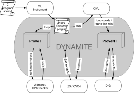
Figure 1. Tools used in DynamiTe.

DynamiTe takes advantage of several existing dynamic, symbolic, and static analysis techniques and tools as shown in Fig. 1. The two main algorithms to check for termination and nontermination mentioned above are the two blocks labeled ProveT and ProveNT, respectively. As shown in the figure, ProveT uses the two tools Ultimate and CPAChecker to verify the inferred ranking functions and obtain counterexamples to improve the inference process. On the other hand, ProveNT uses the CIVL symbolic execution tool to obtain program information such as loop conditions and transition relations, the DIG dynamic invariant generation tool to infer invariants from snapshot traces in order to represent and refine recurrent sets. DynamiTe also uses the Z3 and CVC4 SMT solvers to check if the candidate recurrent sets are valid and if not obtains counterexamples to refine DIG’s inference process.

Our algorithms can work with programs containing sequential and/or nested loops. Our program transformation puts each loop into a separate method and replaces the loop by a call to that method. We then build a call graph of those methods and extract a postorder call sequence from it. We analyze each loop at a time in that order, i.e., the top-down innermost loop will be examined first. We proceed to the next loop in the sequence only when we have learned that the current loop is terminating. Otherwise, we conclude that the whole program does not terminate due to the non-termination of the current loop.

Our main goal in this paper is to develop integrated termination/nontermination algorithms that exploit dynamic analysis to support non-linear programs. However, we also evaluate how DynamiTe performs on linear examples. To this end, we evaluated DynamiTe on the 66 benchmarks from the SV-COMP termination-crafted-lit set of linear arithmetic termination and non-termination problems collected from literature. We compared DynamiTe to Ultimate, because it is one of the most successful termination reasoning tools available. We report Ultimate’s proving time as compared with DynamiTe’s guessing time and DynamiTe’s time to validate guesses. Details are in Section 8. Overall, DynamiTe is roughly an order of magnitude slower than Ultimate on linear benchmarks, owing to the fact that DynamiTe must repeatedly execute the program to collect data. Nonetheless, it’s worth noting that Ultimate is a much more mature tool. In one case, DynamiTe was able to learn a rank function that Ultimate could not. We also show that DynamiTe is competitive for proving non-termination of linear programs, as compared to Ultimate’s ability to generate lasso counterexamples to termination.

For the non-linear case, there are two existing benchmarks: polyrank for termination and Anant for non-termination. However, they only have at-most-quadratic polynomial programs and 10/11 programs in the polyrank benchmark are linear. To make (non)termination reasoning more challenging, we adapted the closely related SV-COMP digbench set of programs for non-linear invariant generation problems to create two new sets of benchmarks called termination-nla and nontermination-nla which we are submitting to SV-COMP. The set termination-nla consists of 37 terminating programs and nontermination-nla consists of 38 non-terminating programs, which were created by adapting (up to sextic degree) non-linear invariants in their loop conditions. Our empirical evaluation shows that DynamiTe can discover and sometimes validate rank functions (in 35 of 37 cases) and recurrent sets (in 33 of 38 cases) for non-linear programs, that are not supported by Ultimate. (Ultimate returns an unsupported error message.)

3. Preliminaries

We denote a program by $P$. We assume, for simplicity, that it has a single set $V$ of variables. We will sometimes use the notation $V^{\prime}$ to mean a second set of primed versions of the same variables, i.e. $V^{\prime}=\{v^{\prime}\mid v\in V\}$, to describe transition relations. We denote by $\Sigma$ set of states which we treat as valuations of the variables $V$, i.e. $\Sigma:V\rightarrow Val$. To represent conditions, we use logical formulae for states, denoted $\mathcal{C}$, where $[\![\mathcal{C}]\!]:\Sigma\rightarrow\mathbb{B}$. We also work with logical state transition relations denoted $\mathcal{T}$, where $[\![\mathcal{T}]\!]\subseteq\Sigma\times\Sigma$. $\mathcal{T}$ can also be presented in the form of logical formulae. As we describe below, program loops can be summarized using these conditions and relations, in a standard way.

Definition 3.1 (Ranking functions).

For a state space $S$, a ranking function $f$ is a total map from $S$ to a well-ordered set with ordering relation $\prec$. A relation $\mathcal{T}\subseteq S\times S$ is well-founded if and only if there exists a ranking function $f$ such that $\forall(s,s^{\prime})\in\mathcal{T}.\ f(s^{\prime})\prec f(s)$.

The existence of a ranking function over the transition relation $\mathcal{T}$ of a loop implies the termination of that loop, as there can be no infinite sequence of states $s_{0},s_{1},\ldots$ such that $\mathcal{T}(s_{i},s_{i+1})$ holds for every $i\geq 0$. This is because for all $i\geq 0$, $f(s_{i+1})\prec f(s_{i})$ and the sequence of states mapped under $f$ cannot be decreasing forever as the image of $f$ is a well-order.

The termination of a loop with a transition relation $\mathcal{T}$ can also be proved by a finite set of ranking functions (or measures) $\mathcal{M}=\{f_{1},\ldots,f_{m}\}$ by showing that the transitive closure of $\mathcal{T}$ is contained in the disjunctively well-founded relation defined from $\mathcal{M}$ (Podelski and Rybalchenko, 2004b). That is, $\mathcal{T}^{+}\subseteq\{(s,s^{\prime})~{}|~{}f_{1}(s^{\prime})\prec f_{1}(s)\vee\ldots\vee f_{m}(s^{\prime})\prec f_{m}(s)\}$.

This validity of the finite set of ranking functions $\mathcal{M}$ for the loop’s termination can be checked via proving safety of the following instrumented loop (i.e., the error is unreachable) (Cook et al., 2006). This check can be performed by a reachability prover such as Ultimate (2020) or CPAchecker (Beyer and Keremoglu, 2011). Below is an illustration for a while loop, whose instrumentation code are put in gray boxes.

⬇

lightgray_dup = False

while C:

lightgrayif _dup:

lightgrayif not ($f_{1}(\hat{x}_{1},...,\hat{x}_{n})>f_{1}(x_{1},...,x_{n})$ and $f_{1}(\hat{x}_{1},...,\hat{x}_{n})\geq 0$):

lightgray$\ldots$

lightgrayif not ($f_{m}(\hat{x}_{1},...,\hat{x}_{n})>f_{m}(x_{1},...,x_{n})$ and $f_{m}(\hat{x}_{1},...,\hat{x}_{n})\geq 0$):

lightgrayERROR: skip

lightgrayif not _dup and *:

lightgray$\hat{x}_{1}=x_{1};...;\hat{x}_{n}=x_{n}$

lightgray_dup = True

B \end{lstlisting}

\end{minipage}

\end{wrapfigure}

\noindent In this instrumented program, a state $\hat{s}$ of the loop is arbitrarily recorded and then for any subsequent state $s$, we check if the transition $(\hat{s},s)$ satisfies at least one ranking function in $\mathcal{M}$. A transition $(\hat{s},s)$ that does not satisfy any ranking function in $\mathcal{M}$, indicates that the transitive closure transition $\mathcal{T}^{+}$ is not a subset of the disjunctively well-founded relation of $\mathcal{M}$. In this case, the error is reached and the termination proof fails. Otherwise, a safe program in which the error is unreachable implies the loop’s termination.

\begin{definition}[Recurrent set]\label{def:rcr}

For sets of states $X$ and transition relation $\mathcal{T}$,

$X$ is a \emph{recurrent set} if

\[\begin{array}{lll}

\textrm{(1) } X\neq \emptyset, &

\textrm{(2) } \Rel \textrm{ is total on } X, &

\textrm{(3) } \textrm{ the image of } \Rel \textrm{ on } X \textrm{ is contained within } X

\end{array}\]

\end{definition}

%We will often work with recurrent sets and transition

%relations described with

%formulas (\eg\ denoted $\mathcal{C}$ and $\mathcal{T}$, respectively).

\diff{The above notion of recurrent sets (\ie\ ‘‘closed recurrent sets’’ in~\cite{Chen2014}) can help to avoid the difficulty and inefficiency of reasoning the $\forall\exists$ alternation in ‘‘open recurrent sets’’~\cite{Gupta2008}, but it cannot support non-determinism without under-approximation. Therefore, our non-termination proofs are restricted to only deterministic programs. Finding under-approximation of non-determinism from concrete possibly-nonterminating snapshots to support non-termination proofs of non-deterministic programs will be our future work. Note that such restriction does not apply to our termination proofs.}

\begin{definition}[Loop summary]

As is typical~\cite{Cook2006}, we will describe loops in terms

of a triple ($\mathcal{T}_{\texttt{stem}},\mathcal{C}_{\texttt{loop}},\mathcal{T}_{\texttt{loop}}$), where

$\mathcal{T}_{\texttt{stem}}$ over-approximates the transition from the entrypoint

of the program up to the loop header,

$\mathcal{C}_{\texttt{loop}}$ over-approximates the condition for entering the loop, and

$\mathcal{T}_{\texttt{loop}}$ over-approximates the transition through the entire body of the

loop back to the header.

\end{definition}’

4. Inferring Ranking Functions for Termination

⬇ 1$\textsf{ProveT}(P,P_{\texttt{instr}},L,\pi_{\texttt{term}})$: 2 rfset = $\{\}$ 3 $\bar{\pi}_{\texttt{mayloop}}$ = $\{\}$ 4 while (True): 5 new_rfset = $\textsf{InferRF}(\pi_{\texttt{term}},L)$ 6 rfset = rfset $\cup$ new_rfset 7 if (IsUnchanged(rfset): 8 return ($\texttt{Unk},\bar{\pi}_{\texttt{mayloop}}$) 9 else: 10 cex = ValidateRFs($P$, rfset) 11 if (not cex): 12 return ($\par,\{\}$) 13 else: 14 inps = GuessInputs($P_{\texttt{instr}}$, cex) 15 $\pi$ = Execute($P_{\texttt{instr}}$, inps) 16 $\pi_{L}$ = Project($\pi,L$) 17 $\pi_{\texttt{base}},\pi_{\texttt{term}},\pi_{\texttt{mayloop}}$ = $\texttt{Partition}(\pi_{L},L)$ 18 $\bar{\pi}_{\texttt{mayloop}}$ = $\bar{\pi}_{\texttt{mayloop}}\cup\pi_{\texttt{mayloop}}$        ⬇ 1$\textsf{InferRF}(\pi_{\texttt{term}},L)$: 2 tcTrans = $\{\}$ 3 for $\tau_{L}$ in $\pi_{\texttt{term}}$: 4 tcTrans = tcTrans $\cup$ GenTCTrans($\tau_{L}$) 5 rfTemplate = $\texttt{GenRFTemplate}(L)$ 6 rfset = $\{\}$ 7 while not IsEmpty(tcTrans): 8 ($s_{1}$, $s_{2}$) = RandPop(tcTrans) 9 $t_{1}$ = rfTemplate($s_{1}$) 10 $t_{2}$ = rfTemplate($s_{2}$) 11 rf = Solve(rfTemplate, $\{t_{1}>t_{2},t_{1}\geq 0\}$) 12 rfset = rfset $\cup$ $\{$rf$\}$ 13 tcTrans.filter(t: NotSatisfied(t, rf)) 14 return rfset

Figure 2. Algorithm ProveT for proving Termination, aided by dynamic inference of candidate ranking functions.

The algorithm for proving termination is summarized as follows, and two of the main subprocedures involved, ProveT and InferRF, are shown in Fig. 2.

ProveT

The procedure ProveT aims to prove the termination of a loop $L$ in an instrumented program $P_{\texttt{instr}}$ by inferring a set of ranking functions from a given set of terminating traces $\pi_{\texttt{term}}$. (We discuss how $P_{\texttt{instr}}$ is built from $P$ in Section 2 and formalize it in Section 7.) The procedure returns either the result Term when the termination proof is successful or otherwise, returns Unk with a set of “possibly non-terminating” traces $\bar{\pi}_{\texttt{mayloop}}$ as a counterexample. Initially, the counterexample $\bar{\pi}_{\texttt{mayloop}}$ and the set of ranking functions rfset are initialised to be empty. The procedure then enters a loop until a valid set of ranking functions is found or until no progress is made when updating the set of ranking functions. Starting with the set of terminating traces $\pi_{\texttt{term}}$, the subprocedure InferRF is called to produce a set of ranking functions that attempts to cover those traces in $\pi_{\texttt{term}}$. The details for this subprocedure is given in the next paragraph. The current set of ranking functions rfset is updated to include the resulting set of ranking functions (new_rfset) from InferRF. The loop in ProveT exits if no new ranking functions were added. Otherwise, the updated set of ranking functions rfset is validated against the original program $P$ via a reachability prover (as is standard (Cook et al., 2006)). If the prover returns no counterexample, which means the validation is successful, ProveT returns Term indicating that the loop $L$ is terminating (via the set of ranking functions rfset). On the other hand, if a counterexample to the set of ranking functions is found, then a new set of inputs is generated. The given program is executed on those new inputs and a set of concrete traces from these executions ($\pi$) is collected. These traces are then projected into the locations of interest in the loop $L$. That is, for each trace $\tau\in\pi$, the projection returns a sequence of states $\tau_{L}$, comprising the state right before the loop, the states reached inside the loop, right after the loop header, and the state at the loop’s exit. Subsequently, the set of these sub-traces ($\pi_{L}$) are partitioned on whether they never enter the loop’s body ($\pi_{\texttt{base}}$), whether they terminate ($\pi_{\texttt{term}}$), and whether they reach the instrumented bound of iterations before terminating, and as such are classified as “possibly non-terminating” ($\pi_{\texttt{mayloop}}$). Finally, the traces in $\pi_{\texttt{mayloop}}$ are added into the counterexample $\bar{\pi}_{\texttt{mayloop}}$ and the procedure repeats the above steps with the new set of terminating traces $\pi_{\texttt{term}}$.

InferRF

This sub-procedure first generates a random sample of pairs of snapshots from the transitive closure of the concrete transition relation as follows. For each terminating trace $\tau_{L}\in\pi_{\texttt{term}}$, with an implicit order of appearance in the trace $\tau_{L}$ present, all combinations $(\sigma_{1},\sigma_{2})$ of the states $\sigma_{1},\sigma_{2}\in\tau_{L}$ are generated, restricted so that $\sigma_{1}$ appears before $\sigma_{2}$ in $\tau_{L}$. The set of these combinations is randomly shuffled into a list, and the first $K$ pairs are selected, with $K$ being a predefined value for the desired size of the sample. All these samples from each trace $\tau_{L}$ are aggregated into the set tcTrans. The subprocedure InferRF also generated a ranking function template, which is of the form $u_{0}+u_{1}\cdot v_{1}+u_{2}\cdot v_{2}+\ldots u_{n}\cdot v_{n}$ for the set of variables $\{v_{1},\ldots,v_{n}\}$ in the loop $L$ and the unknown coefficients $u_{0},u_{1}\ldots,u_{n}$.

While the set tcTrans is non-empty, an element $(s_{1},s_{2})$ is randomly popped, and two instances $t_{1},t_{2}$ of the template are produced for the two respective states $s_{1}$ and $s_{2}$. Given the valuation $\{h^{i}_{1},\ldots,h^{i}_{n}\}$ of the set of variables $\{v_{1},\ldots,v_{n}\}$ in the state $s_{i}$, for $i\in\{1,2\}$, the instance $t_{i}$ is of the form $u_{0}+u_{1}\cdot h^{i}_{1}+u_{2}\cdot h^{i}_{2}+\ldots u_{n}\cdot h^{i}_{n}$. The solver from Z3 is then asked to return values for $u_{0},\ldots,u_{n}$ that satisfy the constraints

$$\begin{array}[]{lcl}u_{0}+\sum_{1\leq j\leq n}u_{j}\cdot h^{1}_{j}>u_{0}+\sum_{1\leq j\leq n}u_{j}\cdot h^{2}_{j},&\;\;\;\textrm{ and }&u_{0}+\sum_{1\leq j\leq n}u_{j}\cdot h^{1}_{j}\geq 0,\end{array}$$

while minimizing the value of $\sum_{0\leq j\leq n}|u_{j}|$. The resulting solution of values for $u_{0},\ldots,u_{n}$ is added as a candidate ranking function to the set rfset of accumulated ranking functions. Any pair of states $(s_{1},s_{2})$ from the random sample of trasitive closure of the transition relation that was constructed earlier, that satisfies the latter candidate ranking function is removed from that sample, and the procedure continues with the remaining ones.

Correctness.

Sub-procedure InferRF terminates since at each iteration of the loop we remove at least one of the pairs $(s_{1},s_{2})$ from tcTrans (line 8 of InferRF), but possibly more (line 13 of InferRF). By construction, each ranking function returned by InferRF handles at least one of the pairs $(s_{1},s_{2})$ in tcTrans. Such a candidate ranking function is only returned by ProveT if it is validated on $P$ by a reachability solver. On the other hand, it is not guaranteed that ProveT will terminate. Because the traces are dynamically generated, and because the transitive closure is sampled randomly, a newly inferred candidate ranking function could potentially only handle few of the possible pairs of states in the actual transitive closure of the loop body. As a result, a new ranking function may be added to the set of possible ranking functions continuously (see line 6 of ProveT).

5. Inferring Recurrent Sets for Non-Termination

⬇ 1$\textsf{ProveNT}(P_{\texttt{instr}},L,\pi_{\texttt{mayloop}})$: 2 ($\mathcal{T}_{\texttt{stem}}$, $\mathcal{C}_{\texttt{loop}}$, $\mathcal{T}_{\texttt{loop}}$) = GetLoopInfo($P_{\texttt{instr}}$, $L$) 3 $\mathcal{C}_{\texttt{mayloop}}$ = DynInfer($\pi_{\texttt{mayloop}}$) 4 # stack of candidate recurrent sets 5 stack S = $\{(0,\mathcal{C}_{\texttt{loop}}),(0,\mathcal{C}_{\texttt{mayloop}})\}$ 6 $\bar{\pi}_{\texttt{term}}$ = $\{\}$ 7 8 while not IsEmpty(S): 9 (depth, $R$) = Pop(S) 10 if (depth>UPPERBOUND or $R(\bar{V}){\centernot\implies}\mathcal{C}_{\texttt{loop}}(\bar{V})$): 11 continue; 12 if $\texttt{IsValid}(R(\bar{V})\wedge\mathcal{T}_{\texttt{loop}}(\bar{V},\bar{V}^{\prime})\implies R(\bar{V}^{\prime}))$: 13 if $\texttt{IsSat}(\mathcal{T}_{\texttt{stem}}(\bar{V}_{0},\bar{V})\wedge R(\bar{V}))$: 14 return ($\texttt{NonTerm},\{\}$) 15 else: 16 $RS,\pi_{\texttt{term}}$ = $\text{{RefineRS}}(R,P_{\texttt{instr}},L,\mathcal{T}_{\texttt{stem}},\mathcal{T}_{\texttt{loop}})$ 17 $\bar{\pi}_{\texttt{term}}$ = $\bar{\pi}_{\texttt{term}}\cup\pi_{\texttt{term}}$ 18 for $R^{\prime}$ in $RS$: 19 S.push($(\text{depth}+1,R^{\prime})$) 20 return ($\texttt{Unk},\bar{\pi}_{\texttt{term}}$)        ⬇ 1$\texttt{RefineRS}(R,P_{\texttt{instr}},L,\mathcal{T}_{\texttt{stem}},\mathcal{T}_{\texttt{loop}})$: 2 $R\text{ as }\bigwedge_{i}R_{i}$ 3 $RS=\{\}$ 4 $\bar{\pi}_{\texttt{term}}$ = $\{\}$ 5 for $R_{i}$ in $R$: 6 $r_{i}=(R(\bar{V})\wedge\mathcal{T}_{\texttt{loop}}(\bar{V},\bar{V}^{\prime})\implies R_{i}(\bar{V}^{\prime}))$ 7 if $\texttt{IsSat}(\neg r_{i})$: 8 inps = $\texttt{GuessInputs}(\mathcal{T}_{\texttt{stem}}(\bar{V}_{0},\bar{V})\wedge\neg r_{i}(\bar{V},\bar{V}^{\prime})$ 9 $\pi$ = Execute($P_{\texttt{instr}}$, inps) 10 $\pi_{L}$ = $\texttt{Project}(\pi,L)$ 11 $\pi_{\texttt{base}},\pi_{\texttt{term}},\pi_{\texttt{mayloop}}$ = Partition($\pi_{L},L$) 12 $\mathcal{C}_{\texttt{term}}$ = $\texttt{DynInfer}(\pi_{\texttt{term}})$ 13 $\mathcal{C}_{\texttt{mayloop}}$ = $\texttt{DynInfer}(\pi_{\texttt{mayloop}})$ 14 $\bar{\pi}_{\texttt{term}}$ = $\bar{\pi}_{\texttt{term}}\cup\pi_{\texttt{term}}$ 15 $\mathcal{C}_{\texttt{term}}\text{ as }\bigwedge_{i}\mathcal{C}_{i}$ 16 for $\mathcal{C}_{i}$ in $\mathcal{C}_{\texttt{term}}$: 17 $RS=RS\cup\{R\wedge\neg\mathcal{C}_{i}\}$ 18 $RS=RS\cup\{\mathcal{C}_{\texttt{mayloop}}\}$ 19 return $(RS,\bar{\pi}_{\texttt{term}})$

Figure 3. Algorithm ProveNT for proving Non-termination, aided by dynamic inference of recurrent sets.

The algorithm ProveNT for proving non-termination is given in Fig. 3. The input is an instrumented program $P_{\texttt{instr}}$, the loop $L$ currently being analysed, and a set $\pi_{\texttt{mayloop}}$ of traces that may be non-terminating. The procedure outputs either that a recurrent set was found (NonTerm), or that such a recurrent set was not found (Unk) together with a set of traces that were found to be terminating. The algorithm is aided by a dynamic sub-procedure RefineRS for guessing candidate recurrent sets, which are then validated.

ProveNT begins by collecting summaries for the loop $L$ in $P$. We use standard techniques (Cook et al., 2006) to represent $L$ in terms of three entities:

• $\mathcal{T}_{\texttt{stem}}$ is a state relation that over-approximates the transition from the entry point of the program up to the entry point of loop $L$.

• $\mathcal{C}_{\texttt{loop}}$ is a state predicate that over-approximates the condition for entering the loop.

• $\mathcal{T}_{\texttt{loop}}$ is a state relation that over-approximates all transitions from the beginning of the body of the loop, back to the loop header.

An illustration of these entities is given in Fig. 4. The algorithm is structured using a stack S as a work list, tracking candidate recurrent sets that will later be examined and possibly refined. To begin with,

Figure 4. Illustration of $\mathcal{T}_{\texttt{stem}}$, $\mathcal{C}_{\texttt{loop}}$ and $\mathcal{T}_{\texttt{loop}}$

we ambitiously select $\mathcal{C}_{\texttt{loop}}$ to be the first candidate recurrent set. The stack element also includes an integer 0, to track the exploration depth, so that we can later bound the search. We also add the condition $\mathcal{C}_{\texttt{mayloop}}$ into the work list S, which is dynamically inferred from the set $\pi_{\texttt{mayloop}}$ of possibly non-terminating traces received from a failed termination proof.

The main loop iterates as long as S is non-empty and no valid recurrent set was found. Popping a candidate $R$ off the stack, if we have gone beyond some upper bound, then we simply ignore $R$ rather than exploring further refinements of $R$. $R$ is also ignored if it doesn’t even imply the loop condition: it could not be a recurrent set. We next use an SMT query IsValid to check whether $R$ is indeed a recurrent set, i.e., Definition LABEL:def:rcr: if $R$ holds of variables $\bar{V}$, and a loop body transition to $\bar{V}^{\prime}$ is possible, then $R$ must hold of $\bar{V}^{\prime}$. If $R$ is a recurrent set, then we check that at least some state in $R$ is reachable from an initial state, using $\mathcal{T}_{\texttt{stem}}$, and if it is we have succeeded in proving the program to be non-terminating. Alternatively, if $R$ is not a recurrent set, we explore further by refining $R$, with respect to this loop, using subprocedure RefineRS discussed below. This subprocedure also collects any terminating traces found during the refinement. Such terminating traces are evidence that the program is terminating, and thus useful for the case where non-termination fails to be proved and the algorithm switches to proving termination.

RefineRS

This subprocedure, shown in Fig. 3, takes as input the current candidate recurrent set $R$ with respect to the loop $L$ and returns a set of new candidate recurrent sets $RS$. The input recurrent set $R$ is assumed to be a conjunction of $\{R_{i}\}_{i\leq k}$, for some $k\in\mathbb{N}$, and it is known that $R$ is not a recurrent set for the transition relation $\mathcal{T}_{\texttt{loop}}$. As such there are two states $\sigma$ and $\sigma^{\prime}$ (i.e. two valuations of the set of variables $\bar{V}$), for which the formula on the left does not hold:

$$\begin{array}[]{ccc}\bigwedge_{i\leq k}R_{i}(\sigma)\land\mathcal{T}_{\texttt{loop}}(\sigma,\sigma^{\prime})\implies\bigwedge_{i\leq k}R_{i}(\sigma^{\prime})&\hfill\hfil&r_{i}=\bigwedge_{i\leq k}R_{i}(\sigma)\land\mathcal{T}_{\texttt{loop}}(\sigma,\sigma^{\prime})\implies R_{i}(\sigma^{\prime})\end{array}$$

Therefore, for at least one of the $i\leq k$, the formula on the right does not hold. The candidate recurrent set $R$ is updated for each such $R_{i}$ as described next. The algorithm proceeds via GuessInputs using SMT to generate solutions $\bar{V}_{0}$ to the formula $\exists\bar{V},\bar{V}^{\prime}\ \mathcal{T}_{\texttt{stem}}(\bar{V}_{0},\bar{V})\wedge\neg r_{i}(\bar{V},\bar{V}^{\prime})$, which are used as inputs to execute $P_{\texttt{instr}}$. Informally, these inputs are witnesses to a path, via $\mathcal{T}_{\texttt{stem}}$, from the initial state to a state on which the recurrent set fails. After the program is executed using the resulting inputs inps and a set of traces is produced as a result. The traces are first projected—to include the instrumented information regarding only the loop $L$ being analyzed—and then partitioned into: the traces $\pi_{\texttt{base}}$ that never enter the loop, traces $\pi_{\texttt{term}}$ that definitely terminate, and traces $\pi_{\texttt{mayloop}}$ that may be non-terminating, as the execution for the latter reached the imposed loop bound. It should be noted that, since any candidate $R$ implies $\mathcal{C}_{\texttt{loop}}$, if the program is deterministic, and assuming soundness of the preceding subprocedures, then the inputs inps will not cause any traces that never enter the loop to be generated, and thus $\pi_{\texttt{base}}$ will be empty. Traces $\pi_{\texttt{term}}$ are used to dynamically infer a condition $\mathcal{C}_{\texttt{term}}$ that captures the set of states reached right after the loop header by those terminating traces and a similar condition $\mathcal{C}_{\texttt{mayloop}}$ is inferred using $\pi_{\texttt{mayloop}}$. The accumulating set $\bar{\pi}_{\texttt{term}}$ is updated to include $\pi_{\texttt{term}}$ and the recurrent set $RS$ is then updated as follows. For every conjunct $\mathcal{C}_{i}$ of $\mathcal{C}_{\texttt{term}}$, $RS$ is updated to include the strengthened candidate recurrent set $R\land\lnot\mathcal{C}_{i}$ in which any states in $\mathcal{C}_{i}$ that is possibly in a terminating trace is excluded from the candidate. The condition $\mathcal{C}_{\texttt{mayloop}}$ is also included as a new candidate recurrent set since it captures all states that are in possibly non-terminating traces. At the end, the procedure RefineRS returns the set of candidate recurrent sets constructed, together with any terminating traces accumulated in $\bar{\pi}_{\texttt{term}}$.

Consider the example to the right with non-linear expressions to illustrate how ProveNT and RefineRS works. The summary of this loop is: $\mathcal{T}_{\texttt{stem}}=\textsf{true}$, $\mathcal{C}_{\texttt{loop}}=t\leq n^{2}+1$, and

⬇

int t, n, m

while (t <= n*n + 1):

t = t + 2*m

n = n + 1

$\mathcal{T}_{\texttt{loop}}=t\leq n^{2}+1\wedge t^{\prime}=t+2m\wedge n^{\prime}=n+1\wedge m^{\prime}=m$. The procedure ProveNT first uses the loop condition $t\leq n^{2}+1$ as a candidate recurrent set and checks if the implication $t\leq n^{2}+1\wedge\mathcal{T}_{\texttt{loop}}\implies t^{\prime}\leq n^{\prime 2}+1$ is valid. As this is not the case, ProveNT invokes RefineRS on this invalid recurrent set to refine it. Then RefineRS finds a set of inputs over the variables $(t,n,m)$ that invalidate the implication, such as $\{(29,-6,-1),(13,-4,0),(1,0,1),(1,-1,2),(0,0,3),(1,1,4),\ldots\}$. The program execution over these inputs produces only terminating traces and a dynamic invariant inference tool, like Dig (Nguyen et al., 2014a, 2012), can generate the condition $m\geq-1$ from the snapshots at the beginning of the loop’s body in those traces. This possibly terminating condition (see $\mathcal{C}_{\texttt{term}}$ in RefineRS) is used to refine the current candidate into a new one $t\leq n^{2}+1\wedge\neg(m\geq-1)$. Unfortunately, this new candidate recurrent set is still invalid and RefineRS generates a new set of inputs from its validity check, that is $\{\ldots,(78,-9,-5),(26,-5,-4),(24,-5,-3),(15,-4,-2)\}$. Again, all these inputs lead to terminating traces, from which a new condition $n\leq m-1\wedge m\leq-2$ can be dynamically inferred. From this new condition, RefineRS returns two new candidate recurrent sets by strengthening the current candidate $t\leq n^{2}+1\wedge\neg(m\geq-1)$:

1. $t\leq n^{2}+1\wedge\neg(m\geq-1)\wedge\neg(n\leq m-1)$, and

2. $t\leq n^{2}+1\wedge\neg(m\geq-1)\wedge\neg(m\leq-2)$.

Finally, the procedure ProveNT determines that the new candidate (1) is a valid recurrent set and returns the result NonTerm.

DynInfer.

We use dynamic invariant inference to guess conditions from terminating traces and potentially non-terminating traces which are then used to refine the invalid candidate recurrent sets. Dynamic invariant generation works, pioneered by the tool Daikon (Ernst et al., 2007; Ernst et al., 2001), learns candidate invariants from program execution traces and templates (e.g., equalities, inequalities). Recent works in dynamic invariant generation are capable of generating very expressive invariants (e.g., nonlinear invariants). In addition, many works integrate dynamic inference with static checking to remove spurious invariants. We use the DIG (Nguyen et al., 2012, 2014a) tool to infer numerical invariants from traces. DIG supports nonlinear equations as well as several other forms of inequalities such as octagonal invariants and max/min-plus invariants. DIG reduces the problem of nonlinear equation solving to linear equation and ussing terms to represent nonlinear polynomials and uses linear constraint solving to find octagonal and max/min-plus invariants. In addition, DIG implements a counterexample-guided invariant generation technique that iteratively infer candidate invariants from program traces and check them using symbolic execution, which, for incorrect invariants, returns counterexamples that are used as traces to help DIG infer better results in the next iteration.

5.1. Correctness

ProveNT

For correctness of the algorithm ProveNT we aim to show that if its output is $(\texttt{\small NonTerm},\{\})$ then there is at least one execution of the program $P$, that leads to a non-terminating execution of the loop $L$ at hand. For what follows, we assume that

1. for any state that satisfies $\mathcal{C}_{\texttt{loop}}$, there is a valid transition from that state in the program $P$,

2. $\mathcal{T}_{\texttt{stem}}$ is an exact representation, or at worst an under-approximation, of the transition from the entrypoint to the loop header, and

3. $\mathcal{T}_{\texttt{loop}}$ is an exact representation, or at worst an over-approximation, of the loop body transition.

The procedure ProveT will declare that the input loop is non-terminating only when both $\texttt{\small IsValid}(R(\bar{V})\wedge\mathcal{T}_{\texttt{loop}}(\bar{V},\bar{V}^{\prime})\implies R(\bar{V}^{\prime}))$ and $\texttt{\small IsSat}(\mathcal{T}_{\texttt{stem}}(\bar{V}_{0},\bar{V})\wedge R(\bar{V}))$ hold (see lines 12 and 13 of ProveNT). In other words,

$$(i)\hskip 5.0pt\exists\bar{V}_{0},\bar{V}\ \mathcal{T}_{\texttt{stem}}(\bar{V}_{0},\bar{V})\wedge R(\bar{V})\hskip 20.0pt\textrm{ and }\hskip 20.0pt(ii)\hskip 5.0pt\forall\bar{V},\bar{V}^{\prime}R(\bar{V})\wedge\mathcal{T}_{\texttt{loop}}(\bar{V},\bar{V}^{\prime})\implies R(\bar{V}^{\prime}).$$

Formula $(ii)$, together with the assumption (3) above implies the condition (3) of Definition LABEL:def:rcr. From formula (i) and the assumption (2) above, there is a state $S^{\prime}$ at the loop header that can be reached from $S$, such that $R(S^{\prime})$ holds which implies that condition (1) of Definition LABEL:def:rcr holds for a reachable state in $P$ from $S$. Finally, given that $R$ implies $\mathcal{C}_{\texttt{loop}}$ (see line 10 of ProveNT), and given the assumption (1) above, it follows that the real transition relation for the loop is total on $R$. Therefore there is a non-terminating execution of $P$ starting from the state $S$. We should note that, given that $\mathcal{T}_{\texttt{stem}}$ is an over-approximation in reality, our implementation could simply check if a witness path exists.

Further, the algorithm terminates, since whenever a new candidate recurrent set $R$ is added the variable depth is increased and the recurrent sets with an accompanying depth of value higher than UPPERBOUND are ignored (see line 10 of ProveNT).

6. An integrated algorithm

We now describe ProveTNT, an algorithm supported with dynamic analysis, that mixes termination and non-termination reasoning, allowing the failed outcomes of one endeavor to provide feedback to the other. In this algorithm, ProveNT consumes the previously ignored argument $\bar{\pi}_{\texttt{mayloop}}$

⬇

1ProveTNT($P$):

2 $P_{\texttt{instr}}$ = Instrument($P$)

3 inps = GenRandomInputs($P_{\texttt{instr}}$)

4 $\pi$ = Execute($P_{\texttt{instr}}$, inps)

5 $\mathcal{L}$ = GetLoopSeq($P_{\texttt{instr}}$)

6

7 for $L$ in $\mathcal{L}$:

8 $\pi_{L}$ = Project($\pi,L$)

9 $\pi_{\texttt{base}},\pi_{\texttt{term}},\pi_{\texttt{mayloop}}$ = Partition($\pi_{L},L$)

10 if $\mathbf{card}(\pi_{\texttt{mayloop}})$ >> $\mathbf{card}(\pi_{\texttt{base}}\cup\pi_{\texttt{term}})$:

11 $r_{nt},\bar{\pi}_{\texttt{term}}$ = ProveNT($P_{\texttt{instr}},L,\pi_{\texttt{mayloop}}$)

12 if $r_{nt}$ is NonTerm:

13 return NonTerm

14 else:

15 $r_{t},\_$ = ProveT($P,P_{\texttt{instr}},L,\pi_{\texttt{term}}\cup\bar{\pi}_{\texttt{term}}$)

16 if $r_{t}$ is Unk:

17 return Unk

18 else:

19 $r_{t},\bar{\pi}_{\texttt{mayloop}}$ = ProveT($P,P_{\texttt{instr}},L,\pi_{\texttt{term}}$)

20 if $r_{t}$ is Unk:

21 $r_{nt},\_$ = ProveNT($P_{\texttt{instr}},L,\pi_{\texttt{mayloop}}{\cup}\bar{\pi}_{\texttt{mayloop}}$)

22 if $r_{nt}$ is NonTerm:

23 return NonTerm

24 else:

25 return Unk

26 return Term

Figure 5. The integrated algorithm for approving termination and non-termination, via mutual feedback.

(a set of potentially non-terminating traces returned by ProveT) and ProveT consumes the previously ignored argument $\bar{\pi}_{\texttt{term}}$ (a set of terminating traces from ProveNT).

The procedure ProveTNT is given in Fig. 5 and begins by instrumenting the input program $P$, generating random initial inputs, and executing the instrumented program on those inputs to get a set $\pi$ of concrete traces. These executions may be used for reasoning about multiple loops in the program, and avoid the need for re-execution. We then iterate over the loops in the program in a post-order fashion, in which the top-down innermost loop will be analyzed first. If that loop is proved to be non-terminating, the procedure returns the result NonTerm immediately. Otherwise, it continues to analyze the next loop in the post-order sequence. At the end, the procedure returns the result Term when all loops in the program are proved to be terminating.

Within each loop $L$ we project on the set of traces, focusing on only those that reach $L$’s header and keeping only the relevant snapshots from the instrumentation on that loop in $\pi_{L}$ (see line 8 in ProveTNT). We then partition $\pi_{L}$ into the three classes of traces $\bar{\pi}_{\texttt{base}},\bar{\pi}_{\texttt{term}},\bar{\pi}_{\texttt{mayloop}}$, similarly to what was described in previous sections. We next make a decision as to whether we should attempt non-termination or termination reasoning first. Our algorithm heuristically chooses which action to perform after comparing the sizes of terminating trace sets ($\bar{\pi}_{\texttt{base}}$ and $\bar{\pi}_{\texttt{term}}$) and the potentially non-terminating one ($\bar{\pi}_{\texttt{mayloop}}$). In our implementation, we decide to prove non-termination first when the number of the potentially non-terminating traces is four times larger than the total size of terminating traces. In the case the algorithm succeeds in proving the chosen analysis, it moves to the next step as described above (i.e. returning NonTerm immediately if ProveNT is chosen or analyzing the next loop if ProveT is chosen). Otherwise, the chosen sub-procedure will return counterexamples in the form of new traces, that can be used, together with the traces collected from running the random inputs, as input to the alternative analysis.

Consider the simple program: while(x>=0): x = x + y. This example conditionally terminates, depending on the initial values of x and y. That is, the loop does not terminate when $\texttt{\small x}{\geq}0$ and $\texttt{\small y}{\geq}0$ and terminates otherwise. Given that the random inputs are evenly-distributed then x is negative in roughly half of the random inputs, on which the loop terminates. From the heuristic for choosing the sub-procedure, ProveTNT may decide to attempt proving termination first. More specifically, in our implementation, we decide to prove non-termination first when the number of the potentially non-terminating traces is four times larger than the total size of terminating traces. The sub-procedure ProveT may find a ranking function such as x from the terminating traces. However, it is not a valid ranking function for all inputs and the validation in ProveT returns counterexamples whose corresponding inputs create potentially non-terminating execution traces, such as $[(\texttt{\small x}{=}0,\texttt{\small y}{=}0),(\texttt{\small x}{=}0,\texttt{\small y}{=}0),\ldots]$, $[(\texttt{\small x}{=}3,\texttt{\small y}{=}1),(\texttt{\small x}{=}4,\texttt{\small y}{=}1),\ldots]$, etc., in which the ranking function x is not decreasing. Since there is no terminating trace generated from those inputs, ProveT gives up and returns such potentially non-terminating execution traces as its counterexample traces. At this point, our ProveTNT algorithm switches gears and uses these counterexample traces as inputs to ProveNT. Finally, ProveNT proceeds on these traces and finds a recurrent set $\texttt{\small x}{\geq}0\wedge\texttt{\small y}{\geq}0$ from them to confirm the loop’s non-termination.

The proving strategy in ProveTNT also helps to overcome the scenario when execution traces from a terminating program, like the simple loop in this program: while(x<1000): x = x + 1. This is wrongly categorized as potentially non-terminating due to the predefined instrumented execution bound (e.g. 500) being reached before the loop terminates. In this example, the execution traces with inputs where $\texttt{\small x}<500$ are considered as potentially non-terminating. Note that on those inputs, the collected traces from that loop are identical to traces collected from the non-terminating loop while True: x = x + 1. If those inputs dominate the set of random inputs then the procedure ProveTNT may attempt proving non-termination first. The sub-procedure ProveNT then starts with the first candidate recurrent set $\texttt{\small x}{<}1000$ and performs a check on it with the implication $\texttt{\small x}{<}1000\wedge\texttt{\small x}^{\prime}=\texttt{\small x}{+}1\implies\texttt{\small x}^{\prime}{<}1000$. The implication does not hold and there is only one input of $\texttt{\small x}{=}999$ and the corresponding terminating trace $[\texttt{\small x}{=}999,\texttt{\small x}{=}1000]$ are generated from it as counterexample. Due to the lack of data, the dynamic inference is not triggered and there is no new candidate recurrent set generated. The procedure ProveTNT then passes that terminating counterexample trace to the sub-procedure ProveT for proving termination. From that trace, ProveT can easily find the ranking function $999-\texttt{\small x}$ to prove the loop’s termination. Interestingly, the ProveT alone cannot prove the termination of this loop due to the lack of terminating traces. This happens since we usually prefer to generate small random inputs and limit the number of them, which may help to reduce the program execution time, for efficiency. In this example, we can try inputs larger than the predefined instrumented bound (i.e. $\texttt{\small x}\geq 500$) but the same problem may occur on other examples if the generated inputs are not large enough. For example, for the same program but with the loop condition replaced with x < 10000, the algorithm would require some inputs where x would be larger than or equal to $9500$.

7. The DynamiTe Tool

We have realized our learning-based algorithms in a new tool called DynamiTe. DynamiTe employs the power of several major existing tools, yet our particular combination of them allow DynamiTe  to do things that none of these tools can achieve individually (see Fig. 1). We found that we were able to use these tools with few modifications and, consequently, our framework allows us to benefit from improvements in those tools or substitute alternatives. For SMT, we use SMTlib and for reachability, we follow the SV-COMP (Beyer, 2020) format. We now discuss some of the key components of the implementation.

We perform two transformations on the input program. For validating our guesses in termination reasoning, we use a standard transformation (Cook et al., 2006) that lets us input candidate rank functions and apply a reachability prover. This is a common technique and we have briefly described it in Sec. 3. The second transformation (described in Section 2) involves (i) instrumenting the program to collect states and traces and (ii) truncating potentially infinite loops. For a formal description of this transformation, see Appendix C.

8. Evaluation

Our main goal of DynamiTe is to improve the state-of-the-art in termination and non-termination reasoning to better support non-linear (NLA) programs. To this end, Sections 8.2 and 8.3 report experimental results on those programs. However, in Section 8.1 we first evaluated DynamiTe to see how it performs on linear programs, particularly in comparison with the state-of-the-art tool UAutomizer from Ultimate Ultimate (2020), which is the winner of the Termination category in the recent Competition on Software Verification (SV-COMP) (Beyer, 2020).

Our experiments were all run on a 20-core Intel(R) Core(TM) i7-6950X CPU @ 3.00GHz. DynamiTe in general take advantages of parallel processing when possible. For example, in termination reasoning, multiple instances of Ultimate’s variants (Automizer and Taipan) and CPAchecker are invoked to validate the termination results. In non-termination reasoning, we use these CPU cores to run the symbolic execution tool CIVL to obtain program information at multiple depths. The dynamic inference tool Dig also computes invariants simultaneously. The timeout for each benchmark program is 400s.

8.1. Linear programs

Although our main goal was to support NLA programs (i.e. expressivity) we nonetheless compared our work against the state-of-the-art termination tool UAutomizer. We ran both UAutomizer and DynamiTe on the 61 termination benchmarks and 5 non-termination benchmarks from the SV-COMP suite termination-crafted-lit, which were used in SV-COMP 2020. Note that this folder contains other benchmarks that are for other properties like overflow.

DynamiTe and Ultimate on LIN Termination Programs from SV-COMP

	DynamiTe	Learning		Validate		Total		UAutomizer
Benchmark	Learned Rank Functions	T(s)	Res	T(s)	Res	T(s)	$\sigma_{5}$	T(s)	Res
AlDaFeGo-SAS2010-easy2-2.c	$z$	7.4	✓	8.0	✓	20.7	1.2	0.4	✓
AlDaFeGo-SAS2010-random2d.c	$N{+}r,-r,r{-}i,x{-}r,i{-}r,N{-}i$	23.8	✓	13.2	✓	52.38	7.9	0.6	✓
AlDaFeGo-SAS2010-wcet2.c	$-i,1{-}i,j,j{-}i,-j,2{-}i$	11.5	✓	121.5	?	148.14	75.3	1.3	✓
BrCoFu-CAV2013-Fig1.c	$n{-}j,j,-i,n{-}i$	28.9	✓	14.2	✓	66.22	22.0	1.5	✓
ChCoGuSaYa-ESOP2008-easy2.c	$z$	3.9	✓	2.8	✓	9.4	0.8	0.4	✓
ChFlMu-SAS2012-Ex3.01.c	$-x{+}z,y,-x$	5.9	✓	4.0	✓	16.34	2.4	2.8	✓
CoSeZu-TACAS2013-Fig8a-mod.c	$-x,x,-K{+}x,K{-}x$	11.7	✓	4.0	✓	18.62	0.9	4.6	✓
HaLaNoRa-SAS2010-Fig1.c		0.0	?	4.9	?	8.94	1.8	29.4	✓
HeHoLePo-ATVA2013-Fig5.c	$x$	2.3	✓	5.8	✓	9.56	0.5	3.8	?
KrShTsWi-CAV2010-Fig1.c	$28{-}x,82{-}x,88{-}x,(\textrm{see below})$	8.9	✓	6.0	?	14.66	1.5	3.9	✓
LeHe-TACAS2014-Ex1.c	$q$	2.2	✓	2.9	✓	8.78	1.8	0.5	✓
PoRy-TACAS2011-Fig1.c	$y$	2.4	✓	4.6	✓	8.76	0.9	0.3	✓
Ur-WST2013-Fig2.c	$-x1,-x1+5{\cdot}x2,(\textrm{see below})$	14.2	✓	12.5	✓	32.78	5.7	1.6	✓
cstrcspn.c		–	–	–	–	2	0.2	90.3	✓
genady.c	$i$	0.1	✓	7.4	✓	9.78	1.6	0.4	✓

…      (Results of for the other 46 benchmarks in Appendix A.   

$$\begin{array}[]{lll}\textrm{KrShTsWi-CAV2010-Fig1.c:}&28{-}x,82{-}x,88{-}x,90{-}x,104{-}x,118{-}x,144{-}x,156{-}x,\\ &212{-}x,214{-}x,228{-}x,234{-}x,246{-}x\\ \textrm{Urban-WST2013-Fig2.c:}&-x1,-x1+5{\cdot}x2,-x1+6{\cdot}x2,-x1+7{\cdot}x2,-x1+8{\cdot}x2,-x1+9{\cdot}x2,-x1+10{\cdot}x2,-x2\end{array}$$

Figure 6. Results of applying UAutomizer and DynamiTe on the 61 termination benchmarks from SV-COMP termination-crafted-lit. For lack of space, we only show 15 rows (every 4th row); the rest are shown in Appendix A. Names are abbreviated; see Appendix B. ${\bf?}$ indicates unknown results.

Terminating Linear programs

The results of the experiments on these programs are shown in Table 8. Since DynamiTe is nondeterministic, we ran our experiments 5 times. We depict the ranking functions learned by DynamiTe in the second column, taken from the first iteration of DynamiTe. If a benchmark program has more than one loop, we report the ranking functions learned from the last analyzed loop. We also break down the overall time (and result) of DynamiTe into time spent to learn ranking functions versus validate them. Finally, we report the Total time, averaged over 5 runs, as well as the standard deviation $\sigma_{5}$.

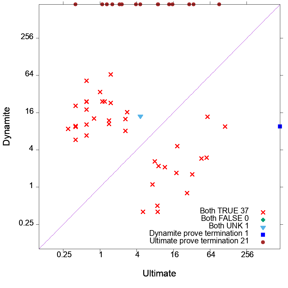
Figure 7. Visual comparison between DynamiTe and UAutomizer on linear termination benchmarks.

In the last two columns, we show the time and result of UAutomizer. These results are also visualized in the plot in Fig. 7. The results show that UAutomizer often performs much faster than DynamiTe on these linear examples, owing largely to the fact that DynamiTe must execute the program many times (on the newly generated inputs), as is typically the case for data-driven strategies (Nguyen et al., 2017a). Nonetheless, the results show that DynamiTe is competitive. In most benchmark programs, DynamiTe can learn useful ranking functions from their terminating traces. For ranking functions that cannot be validated by the reachability provers, we manually checked if they are valid with respect to the observed terminating traces. We found that some of them are the desired ranking functions to prove the programs’ termination while the others are still in good progress so that we could infer the desired ranking functions from their validation’s counterexamples. There are no ranking functions learned from unsupported recursive programs and string-manipulating programs. We also found that DynamiTe was able to infer a ranking function for the program HeHoLePo-ATVA2013-Fig5.c, which can be validated successfully, while UAutomizer cannot. It is worth noting that UAutomizer is a very mature tool, with contributions from multiple researchers/developers, has been applied in industrial settings, and has consistently performed well in the SV-COMP Termination categories. By contrast, DynamiTe is still in its infancy. Furthermore, we will soon discuss non-linear programs, a class of programs not currently supported by UAutomizer.

Non-Terminating Linear programs

Of the termination-crafted-lit SV-COMP suite, only 5 benchmarks were for non-termination. We ran DynamiTe and Ultimate on them; the results are given in Fig. 8. Again we report the mean and standard deviation over 5 runs. In all cases, UAutomizer was able to generate a lasso counterexample to termination. DynamiTe was able to produce a validated recurrent set in 3 programs with UPPERBOUND=3 in ProveNT. The program HeJhMaSu-POPL2002-LockEx.c has a nondeterministic loop condition so that $True$is its trivially valid recurrent set. Therefore, there is no cost for learning recurrent sets in these programs. On the other hand, the program ChCoFuNiHe-TACAS2014-Intro.c has a nondeterministic assignment in its loop body so that while the loop condition is a (closed) recurrent set, it cannot be validated without an underapproximation to restrict the choice of nondeterministic values in that assignment. The two programs Ur-WST2013-Fig1.c and Velroyen.c have many branches in their loop bodies but only some of them were taken by the symbolic execution tool to build the loop summaries. Unfortunately, in Ur-WST2013-Fig1.c, the non-terminating branch was missing so that DynamiTe cannot find any valid recurrent set from the other (terminating) branches in the summary.

DynamiTe and Ultimate on LIN Non-termination Programs from SV-COMP

	DynamiTe	Learning		Validate		Total		UAutomizer
Benchmark	Learned Rec. Sets	T(s)	Res	T(s)	Res	T(s)	$\sigma_{5}$	T(s)	Res
BrMaSi-CAV2005-Fig1-mod.c	$y1{\neq}y2\wedge y2=0$	11.7	✓	8.9	✓	44.3	1.7	0.1	$\chi$
ChCoFuNiHe-TACAS2014-Intro.c		5.8	?	2.7	?	38.68	5.4	0.2	$\chi$
HeJhMaSu-POPL2002-LockEx.c	$True$	0.0	✓	0.1	✓	17.4	0.1	0.1	$\chi$
Ur-WST2013-Fig1.c		6.8	?	0.8	?	17.7	1.8	0.4	$\chi$
Velroyen.c	$x{\neq}0$	0.0	✓	0.1	✓	12.1	0.7	2.2	$\chi$

Figure 8. Results of applying ultimate and DynamiTe on the 5 non-termination benchmarks from SV-COMP termination-crafted-lit. Ultimate returned “incorrect,” indicating that it had found a non-terminating lasso to disprove termination.

8.2. Termination of NLA programs

Currently, we lack challenging benchmark suites for termination of non-linear programs. The existing polyrank benchmark (Bradley et al., 2005b) has only one (quadratic) polynomial program. The other programs in polyrank are linear and many of them were included into the SV-COMP termination-crafted-lit suite. DynamiTe can prove the termination of 8/11 benchmarks (see Fig. 8.1) by inferring multiple linear ranking functions, instead of a single non-linear ranking function, and successfully validating them with Ultimate or CPAchecker. For the remaining 3 examples, DynamiTe was able to infer the correct ranking functions, but the validators could not validate them before timeout. In order to better evaluate the tool, we adapted an existing non-linear testsuite from SV-COMP called nla-digbench which consists of 28 programs implementing mathematical functions such as intdiv, gcd, lcm, power. Although these programs are relatively small (under 50 LoCs) they contain nontrivial structures such as nested loops and nonlinear invariant properties. To the best of our knowledge, nla-digbench contains the largest number of programs containing nonlinear arithmetic. These programs have also been used to evaluate other numerical invariant systems (Yao et al., 2020; Rodríguez-Carbonell and Kapur, 2007b).

However, these benchmarks are for invariant generation rather than termination and most of them are linear programs (with non-linear invariant properties). We therefore adapted these benchmarks to make them suitable non-linear examples for termination. For each benchmark, we manually examined the behavior of the program. The benchmarks contain commented nonlinear assertions, that illustrate the need for non-linear reasoning. For example, bresenham1 contains the assertion 2*Y*x - 2*X*y - X + 2*Y - v == 0. We adapted these assertions to be loop conditions in various ways, creating one or more termination challenge programs. We typically geared the loop condition to the assertion. In this case, we used the invariant that the LHS is 0 and added an additional term +c that increased on each iteration, and made the loop condition bounded by a variable k. For example, from the bresenham1 program, we created a new program in which the loop condition is 2*Y*x - 2*X*y - X + 2*Y - v + c <= k. In other cases, we introduced new variables and had them be integrated by other expressions that we knew to be monotonically increasing or replace variables and numbers with non-linear expressions that are equal to them. We have made these 38 benchmarks available in the supplemental materials (DynamiTe, 2020) and will issue a pull request to submit them to the SV-COMP benchmark repository.

The results of applying DynamiTe to these benchmarks is given in Fig. 8.1. For each benchmark, we give a brief description of the mathematical behaviors of the program in the second column. Based on the results, we display the output list of inferred ranking functions, as well as a breakdown of the time it took to learn versus validate them. As mentioned in the previous section, we use Ultimate and CPAchecker for validation. In 34 of the 38 benchmarks, DynamiTe was able to guess ranking functions. The ranking functions derived from 8 of those 32 benchmarks can be validated. For those ranking functions that cannot be validated by the existing safety provers, we manually inspected them and confirmed they were correct. In the remaining 4 cases, the program cohencu4 is non-terminating because the increment statement c++ was unintentionally not added. Therefore, there are no terminating traces to learn ranking functions. After fixing that problem, DynamiTe can infer the desired ranking functions for this program successfully. The 2 programs freire1 and knuth-nosqrt are originally floating-point programs but were intentionally transformed to integer programs. However, the invariant assertions in the original benchmarks is no longer valid in our adapted benchmark programs. Therefore, the desired ranking functions cannot be found from them. The last program knuth still has the use of sqrt function which is not supported by our CIL instrumentation. It is worth noting that UAutomizer cannot handle these benchmarks. In addition, since the validation get stuck on most benchmarks, we do not report the total time in Fig. 8.1.

DynamiTe on NLA Termination Programs adapted from SV-COMP

Figure 9. Results of applying DynamiTe to the benchmark suite polyrank.

DynamiTe on NLA Termination Programs adapted from SV-COMP

Full RF for	egcd3:	$c+-v,v,-37\cdot b+-d,-293\cdot b+-d,-2341\cdot b+-d,-18725\cdot b+-d,-37449\cdot b+c+-d,10083\cdot c+-d,322639\cdot c+-d,2581111\cdot c+-d,-1677722\cdot b+-d$
	freire1:	$-1\cdot r+12\cdot a+3\cdot k,-1\cdot r+19\cdot a,-1\cdot r+28\cdot a+3\cdot k,-1\cdot r+2\cdot k,-1\cdot r+-1\cdot a,-1\cdot r+-2\cdot a,-1\cdot r+-16\cdot a,-1\cdot r+25\cdot k,-1\cdot r+34\cdot k,-1\cdot r+38\cdot k,-1\cdot r+40\cdot k,-1\cdot r+44\cdot k,-1\cdot r+-19\cdot a,-1\cdot r+89\cdot k,-1\cdot r+105\cdot k,-1\cdot r+154\cdot k,-1\cdot r+186\cdot a$

Figure 10. Results of applying DynamiTe to our new benchmark suite of NLA termination challenge problems. For egcd3 and geo1 the full set of ranking functions are below the table.

8.3. Non-Termination of NLA programs

We first apply DynamiTe to the existing non-linear non-termination benchmark Anant (Cook et al., 2014). The benchmark is a set of quadratic polynomial programs and some of them have non-determinism and divisions. The result of applying DynamiTe on this benchmark is given in Fig. 8.1. DynamiTe can prove the non-termination of 4 benchmarks that (Cook et al., 2014) cannot handle. However, there are 10 benchmarks that DynamiTe cannot handle, due to non-determinism (4), overfitting invariants (1), overflow (1), and problems in SMT solvers (2) or in symbolic execution (2). This result shows that our dynamic approach is orthogonal to the existing static techniques for proving non-termination of (non-linear) programs.

In addition to the benchmark Anant, we also adapted SV-COMP nla-digbench suite to create NLA non-termination challenge programs (e.g. up-to-sextic polynomial programs). (These are also available in the supplementary materials and will be submitted to SV-COMP.) The results of applying DynamiTe on this benchmark are given in Fig. 8.1. Out of the 39 benchmarks, DynamiTe was able to generate a recurrence set for 34 programs.

Interestingly, we found that, for non-termination, our algorithm’s semantic extraction of the first candidate recurrent set from the loop condition already provides a good guess to start with. Consequently, in 28 cases, dynamic analysis was actually unnecessary because our algorithm could already use the loop condition to guide guessing for a recurrent set. This is in contrast with termination, where we don’t have have any semantic information to provide a starting guess for rank functions. However, in 5 cases, dynamic refinement was necessary where the loop conditions are not the existing invariant assertions in the original benchmark programs.

DynamiTe on NLA Non-Termination Programs from Anant

Figure 11. Results of applying DynamiTe to the benchmark suite Anant of NLA non-termination problems.

DynamiTe on NLA Non-Termination Programs adapted from SV-COMP

Figure 12. Results of applying DynamiTe to our new benchmark suite of NLA termination challenge problems.

DynamiTe’s ProveTNT Algorithm on NLA Term. & Non-Term. Programs adapted from SVCOMP

&    

Figure 13. Results of applying DynamiTe to a mix of terminating and non-terminating examples.

8.4. Integrated Algorithm: Discriminating between termination and non-termination

We experimented with ProveTNT to evaluate (a) whether the algorithm is able to discriminate programs that terminate from those that non-terminate and (b) whether feedback from a failed attempt to prove termination can inform a proof of non-termination and vice-versa. For (a), we jumbled together all of the NLA benchmarks and ran the integrated algorithm on them. The results are given in Fig. 8.1. For these benchmarks we note the number of loops (#L). We also indicate whether a guess was made of either a recurrent set (rcr) or a ranking function (rf). ProveTNT makes an initial guess whether to pursue termination or non-termination and if the choice fails, “switches” to the opposite tack. We report the number of switches (#Sw), as well as the final validated conclusion and the total time.

For the vast majority of the examples, there are no switches, which means the initial choice (based on dynamic execution sampling the instrumented program) was was a good one, or that ProveTNT timed out before it could validate a guess. In 16 of the 77 benchmarks, a switch was made at least once. As compared with Fig. 8.1 (NLA Termination) and Fig. 8.1 (NLA Non-termination), more timeouts occur here. However, the comparison is a little unfair: in the earlier experiments we already knew the conclusion (T versus NT) so we aimed DynamiTe toward the prize.

For ProveTNT, one pitfall is that a wrong initial choice could lead to time spent attempting to validate a ranking function, when it should be spent pursing recurrent sets (or vice-versa). A first attack against this problem is to improve the first guess: the better the initial guess, the closer the results come to those in Fig. 8.1 and Fig. 8.1. A naïve strategy could be to add a timeout to validation. Another could be to parallelize, pursuing termination and non-termination concurrently. The downside of parallelization, is that one cannot use the output of one failed endeavor to inform the other. ProveTNT takes an alternate strategy, as dicussed in Section 6: pursue one and, if it fails, exploit the information from the counter example to expedite the alternative. In the worst case, this at least improves over running the two strategies sequentially. In Section 6 we gave two examples that demonstrate where the integrated strategy helps.

8.5. Discussion

Unlike static analysis techniques, our dynamic analysis technique executes the programs to collect data in the form of snapshots at several program locations. In some cases, the time to execute the programs and process their raw output is significant, especially on programs with high-complexity or programs with a large number of parameters which require a large number of random inputs to maintain the data’s diversity. On the other hand, when there is not enough data, overfitting may occur. In proving non-termination, overfitting can make the dynamically inferred conditions too strong to refine a recurrent set. In proving termination, overfitting may create a large number of ranking functions and overwhelm the validation tools. We also have a problem with branching in the loop body where the loop summary returned by the symbolic execution is imprecise since some branches are not taken. That imprecision affects the refinement of candidate recurrent sets.

On the other hand, our dynamic analysis has some advantages that static analysis does not have. For example, we can find a reliable set of ranking functions from known terminating traces at the beginning so we can avoid many expensive validation steps whereas static analysis techniques require many of them to refine the ranking function set from scratch.

9. Related Work

Inference of non-linear invariants.

Nonlinear polynomial relations arise in many safety-and security-critical applications. For example, the Astrée analyzer, which has been applied to verify the absence of errors in the Airbus A340/A380 avionic systems (Blanchet et al., 2003), implements the ellipsoid abstract domain (Feret, 2004) to represent and analyze a class of quadratic inequalities.

Rodríguez-Carbonell and Kapur (2007b, a) used abstract interpretation to infer nonlinear equalities. They first observe that a set of polynomial invariants form the algebraic structure of an ideal, then compute the polynomial invariants using Grobner basis and operations over ideals based on the structure of the program until a fixed point is reached. The approach is restricted to non-nested loops and programs with assignments and loop guards expressible as polynomial equalities. The SPEED project (Gulwani, 2009; Gulwani et al., 2009) uses a numerical abstract domain (Gulavani and Gulwani, 2008) to compute disjunctive and non-linear invariants representing runtime complexity bounds. The numerical domain uses operators such as max to represent disjunction and constraints over various operators using inference rules to represent nonlinear operators.

The well-known dynamic invariant tool Daikon (Ernst et al., 2007; Ernst et al., 2001) infers candidate invariants under various templates over concrete program states. The tool comes with a large set of templates which it tests against observed traces, removing those that fail, and return the remaining ones as candidate invariants. DIG (Nguyen et al., 2014a), which is used by DynamiTe  focuses on numerical invariants and therefore can compute more expressive (e.g., nonlinear) numerical relations than those supported by Daikon’s templates.

More recently, Yao et al. (2020) described a method for inferring invariants through a form of neural networks. The technique uses a Continous Logic Network to learn SMT formulas directly from program traces. The authors show that this approach can learn more general nonlinear invariants (equalities, inequalities, and disjunction).

There are several hybrid works in the form of guessing and checking invariants. In Sharma et al. (2013), “guess” component infers nonlinear equalities using the similar equation solving technique in DIG and the “check” component uses the Z3 SMT solver. Counterexamples from the checker are used to produce more traces to infer better invariants. The works from NumInv (Nguyen et al., 2017a) and SymInfer (Nguyen et al., 2017c) combined the dynamic analyis from DIG to infer nonlinear invariants with symbolic execution to remove spurious results.

PIE (Padhi et al., 2016) and ICE (Garg et al., 2014) also use an guess and check approach to infer invariants to prove a given specification. To prove a property, PIE iteratively infers and refined invariants by constructing necessary predicates to separate (good) states satisfying the property and (bad) states violating that property. ICE uses a decision learning algorithm to guess inductive invariants over predicates sepa- rating good and bad states. The checker produces good, bad, and “implication” counterexamples to help learn more precise invariants.

Termination

Today, numerous theories, techniques, and tools exist for proving termination and non-termination (Podelski and Rybalchenko, 2004a; Giesl et al., 2004; Cook et al., 2006, 2011; Cousot and Cousot, 2012; Dietsch et al., 2015). Tools include Terminator (Cook et al., 2006), Ultimate Automizer (Ultimate, 2020), HipTNT+ (Le et al., 2015), FuncTion (2020), CPAChecker (2020), and AProVE (2020). There is even a category on termination in the Software Verification Competition (SV-COMP) (Beyer, 2020). Along the way, some have shown methods for conditional termination, whereby preconditions are found that specify the portion of traces that terminate (Cook et al., 2008; Le et al., 2015). Another active line of research has focused on flavors of ranking functions, including piece-wise (Urban, 2013), ordinals (Urban and Miné, 2014), size-change (Lee et al., 2001), and lexicographic (Bradley et al., 2005a). Babić et al. (2007) focused on proving termination of a restricted class of non-linear loops, called NAW loops, which have special properties to allow their termination to be proved via analyzing the divergence of variables influencing the loop conditions.

Bradley et al. (2005b, a) focused on the class of polynomial loops from which finite different trees can be derived. However, the techniques could not work on examples with infinite difference trees.

⬇

if x >= 0:

while x * x <= 100:

x = 2 * x + 1

For example, to prove the termination of the program on the right, those techniques construct a difference tree whose root is the expression 100 - x * x in the loop condition. Since the tree is infinite, they could not prove the program’s termination. DynamiTe can derive the ranking function 10 - x from concrete snapshots of that example, which is sufficient to prove its termination.

A number of works have exploited dynamic information to inform termination reasoning. Nori and Sharma (2013) showed that linear regression can be used to dynamically infer bounds of program loops from test suites and these bounds imply termination. They then attempt to validate those bounds and use counterexamples to improve the precision of inference. By using the disjunctive well-foundedness in the termination proofs, DynamiTe can prove the termination of examples in (Nori and Sharma, 2013) which have a disjunctive or non-linear bound with only simple linear ranking functions. Nguyen et al. (2019) describe runtime contracts for enforcing termination, using the size-change strategy for termination.

Several static techniques are able to infer polynomial resource bounds (Hoffmann and Hofmann, 2010b, a; Hoffmann et al., 2011). The TiML functional language (Wang et al., 2017) allows a user to specify time complexity as types and then uses type checking to verify the specified complexity. The WISE tool (Burnim et al., 2009) uses concolic execution to search for a path policy that leads to an execution path with high resource usage.

Non-Termination

Along the line of research on proving non-termination, Gupta et al. (2008) introduced a constraint solving technique to find recurrent sets of non-terminating loops. Later, Chen et al. (2014) strengthened the concept of recurrent sets to “closed” recurrent sets so that they can reduce the non-termination problem to safety proving and support more nondeterministic programs.

Cook et al. (2014) proved non-termination of non-linear programs by soundly over-approximating the programs to nondeterministic linear programs and then using Chen et al. (2014) approach to disprove their termination. However, since the technique searches for linear recurrent sets via Farkas’ lemma on the abstract linear programs, it cannot generate recurrent sets described by non-linear equations. For example, in the benchmarks from Figure 8.1, there were only 5 cases where DynamiTe learned a linear recurrent set and in roughly half of the cases, DynamiTe learned a non-linear recurrent set, which could not be found using the Cook et al. (2014) approach. Therefore, while we are able to leverage ongoing advances in non-linear invariant generation techniques (a growing area of research), the Cook et al. (2014) approach cannot. In addition, Cook et al. (2014) build over-approximation by using an abstract interpreter, such as Interproc, which usually does not perform well on non-linear programs. As shown in Section 8.3, DynamiTe can prove the non-termination of all 4 Anant benchmarks in (Cook et al., 2014) that they cannot handle.

Frohn and Giesl (2019) utilized recurrence relation solvers to replace loops whose non-termination cannot be proved by loop-free transitions in finding feasible paths to a non-terminating loop. The technique relies on recurrence relation solvers, whose supporting forms of recurrence relations are restricted. For example, the approach cannot prove the non-termination of the p3 program in the aforementioned non-linear Anant benchmarks while DynamiTe can.

There are some other approaches that attempt to reason program termination and non-termination at the same time. Harris et al. (2010) introduced a technique that maintains an over- and under-approximation for alternatively proving termination or non-termination of a program. Le et al. (2014) proposed a resource logic which can uniformly specify and verify preconditions of program termination and non-termination. Later, Le et al. (2015) introduced a second-order constraint-based technique to derive termination summary in the form of that logic automatically. However, they cannot handle non-linear programs.

10. Conclusion

We have shown that dynamic strategies for discovering invariants and sampling transitive closure can be incorporated with static refinement into an overall framework for proving termination or non-termination of nonlinear programs. DynamiTe (2020) is publicly available and the new benchmark suites nla-term and nla-nonterm will soon be submitted to SV-COMP. While DynamiTe already exploits concurrency by simultaneously attempting validation with CPAchecker and Ultimate, as well as within DIG, one avenue for improvement is to parallelize ProveTNT.

Acknowledgment

We thank the anonymous reviewers for the helpful feedback. Ton Chanh Le, Timos Antonopoulos, and Eric Koskinen are supported by the Office of Naval Research under Grant N00014-17-1-2787. ThanhVu Nguyen is supported by the National Science Foundation under Grant CCF-1948536 and the Army Research Office under Grant W911NF-19-1-0054.

Appendix A Full version of Fig. 8

DynamiTe and Ultimate on LIN Termination Programs from SVCOMP

$$\begin{array}[]{lll}\textrm{AlDaFeGo-SAS2010-easy1}:&-x,-x+14\cdot z,-x+18\cdot z,-x+22\cdot z,-x+30\cdot z,-x+-2\cdot z,-x+-3\cdot z,-x+-4\cdot z,\\ &-x+-5\cdot z,-x+-6\cdot z,-x+-17\cdot z,25+-x,29+-x,36+-x,37+-x,-x+-38\cdot z\\ \textrm{ChCoGuSaYa-ESOP2008-easy1}:&-x+-z,-x+3\cdot z,-x+4\cdot z,-x+-2\cdot z,-x+-3\cdot z,-x+-4\cdot z,-x+-5\cdot z,-x+-6\cdot z,\\ &-x+-9\cdot z,-x+-22\cdot z,-x+5\cdot z,-x+7\cdot z,-x+15\cdot z,-x+16\cdot z,15+-x,21+-x,\\ &25+-x,34+-x,-x+36\cdot z\\ \textrm{KrShTsWi-CAV2010-Fig1.c}&28+-x,82+-x,88+-x,90+-x,104+-x,118+-x,144+-x,156+-x,212+-x,214+-x,\\ &228+-x,234+-x,246+-x\\ \textrm{Urban-WST2013-Fig2.c}:&-x1,-x1+5\cdot x2,-x1+6\cdot x2,-x1+7\cdot x2,-x1+8\cdot x2,-x1+9\cdot x2,-x1+10\cdot x2,-x2\end{array}$$

Appendix B Naming abbreviations for termination-crafted-lit

Appendix C Transformation for tracing and truncation

For simplicity, we define this transformation in terms of the widely used notion of control flow automata (CFA):

Definition C.1 (Control-flow automaton (Henzinger et al., 2002)).

A (deterministic) control flow automaton denoted $\mathcal{A}$, is a tuple $\mathcal{A}=\langle Q,q_{0},X,s,\xrightarrow{\,}\rangle$ where $Q$ is a finite set of control locations and $q_{0}$ is the initial control location, $X$ is a finite set of typed variables, $s$ is the statement language and $\xrightarrow{\,}\subseteq Q\times s\times Q$ is a finite set of labeled edges.

The statement language $s$ involves loop/branch-free code, with assume statements. We provide the following standard definitions of CFA semantics. We define a valuation of variables $\theta:X\rightarrow\mathit{Val}$ to be a mapping from variable names to values. Let $\Theta$ be the set of all valuations. The notation $\theta^{\prime}\in[\![s]\!]\theta$ means that executing statement $s$, using the values given in $\theta$, leads to a new valuation $\theta^{\prime}$, mapping variables $X$ to new values. Notations $[\![e]\!]\theta$ and $[\![b]\!]\theta$ represent side-effect free numeric and boolean valuations, respectively. We assume that for every $\theta,s$, that $[\![s]\!]\theta$ is computed in finite time. The automaton edges, along with $[\![s]\!]$, give rise to possible transitions, denoted $(q,\theta)\xrightarrow{s}(q^{\prime},\theta^{\prime})$ (we omit these rules for lack of space. A run of a CFA is an alternation of automaton states and valuations: $r=q_{0},\theta_{0},q_{1},\theta_{1},q_{2},\dots$ such that $\forall i\geq 0.\ (q_{i},\theta_{i})\xrightarrow{s}(q_{i+1},\theta_{i+1})$.

We now describe the instrumentation and truncation on CFAs. First, we introduce a new statement ${\bf vtrace}^{i}_{\texttt{pre}}$, that is identical to skip, except that it has a side effect output of the tuple $(pre,i,x_{0},\ldots,x_{n})$ where $i$ is the loop identifier and $pre$ indicates that the values come from the location right before the loop $i$’s header. Similarly, we introduce statements ${\bf vtrace}^{i}_{\texttt{body}}$ for the location right before the loop $i$’s body and ${\bf vtrace}^{i}_{\texttt{post}}$ for the location at the loop’s exit.

Definition C.2 (Truncation and tracing).

We transform the input program CFA $\mathcal{A}$ to an output CFA $\mathcal{A}^{\prime}$. For every loop $i$, having an entry edge from a state $q$ to header node $q_{head}$, we make the following transformation.

$$\begin{array}[]{lcl}\left\{\begin{array}[]{l}q\xrightarrow{s}q_{head}\\ q_{head}\xrightarrow{\texttt{assume}(b)}q_{body}\\ \;\;\;q_{body}\cdots\xrightarrow{}q_{head}\\ q_{head}\xrightarrow{\texttt{assume}(\neg b)}q_{exit}\\ \end{array}\right.&\mapsto&\left\{\begin{array}[]{l}q\xrightarrow{s}q^{\prime}\xrightarrow{\texttt{\_ctr}_{i}=0\texttt{\small; }{\bf vtrace}^{i}_{\texttt{pre}}}q_{head},\qquad q_{head}\xrightarrow{\texttt{assume}(b)}q^{\prime\prime}\\ q^{\prime\prime}\xrightarrow{\texttt{assume}(\texttt{\_ctr}_{i}=\texttt{\_bnd}_{i})}q_{abort}\\ q^{\prime\prime}\xrightarrow{\texttt{assume}(\texttt{\_ctr}_{i}\neq\texttt{\_bnd}_{i});\texttt{\_ctr}_{i}++;}q^{\prime\prime\prime}\xrightarrow{{\bf vtrace}^{i}_{\texttt{body}}}q_{body}\cdots\xrightarrow{}q_{head}\\ q_{head}\xrightarrow{\texttt{assume}(\neg b)}q^{\prime\prime\prime\prime}\xrightarrow{{\bf vtrace}^{i}_{\texttt{post}}}q_{exit}\\ \end{array}\right.\end{array}$$

where primed states $q^{\prime},q^{\prime\prime},$ etc. are fresh states and $q_{abort}$ corresponds to the exit of main.

Intuitively the transformation consists of two parts: (i) Adding an ${\bf vtrace}^{i}_{\texttt{pre}}$ just before the loop, ${\bf vtrace}^{i}_{\texttt{body}}$ at the beginning of the loop body, and ${\bf vtrace}^{i}_{\texttt{post}}$ just outside of the loop. (ii) Introducing a counter $\texttt{\_ctr}_{i}$ specific to the loop, that is initialized to 0 before the loop, incremented on each iteration of the loop and, if ever the counter reaches the predefined bound $\texttt{\_bnd}_{i}$ for the loop, control may break out of the loop (even if the original loop’s condition may hold) and immediately exit main. Counter instrumentation is done in other contexts (Gulwani et al., 2009).

References

- (1)
- AProVE (2020) AProVE. 2020. AProVE: Automated Program Verification Environment. http://aprove.informatik.rwth-aachen.de/.
- Babić et al. (2007) Domagoj Babić, Alan J. Hu, Zvonimir Rakamaric, and Byron Cook. 2007. Proving Termination by Divergence. In Fifth IEEE International Conference on Software Engineering and Formal Methods (SEFM 2007), 10-14 September 2007, London, England, UK. IEEE Computer Society, 93–102. https://doi.org/10.1109/SEFM.2007.32
- Barrett et al. (2011) Clark Barrett, Christopher L. Conway, Morgan Deters, Liana Hadarean, Dejan Jovanovi’c, Tim King, Andrew Reynolds, and Cesare Tinelli. 2011. CVC4. In Proceedings of the 23rd International Conference on Computer Aided Verification (CAV ’11) (Lecture Notes in Computer Science), Ganesh Gopalakrishnan and Shaz Qadeer (Eds.), Vol. 6806. Springer, 171–177. Snowbird, Utah.
- Beyer (2020) Dirk Beyer. 2020. Advances in Automatic Software Verification: SV-COMP 2020. In Tools and Algorithms for the Construction and Analysis of Systems - 26th International Conference, TACAS 2020, Held as Part of the European Joint Conferences on Theory and Practice of Software, ETAPS 2020, Dublin, Ireland, April 25-30, 2020, Proceedings, Part II (Lecture Notes in Computer Science), Armin Biere and David Parker (Eds.), Vol. 12079. Springer, 347–367. https://doi.org/10.1007/978-3-030-45237-7_21
- Beyer and Keremoglu (2011) Dirk Beyer and M Erkan Keremoglu. 2011. CPAchecker: A tool for configurable software verification. In International Conference on Computer Aided Verification. Springer, 184–190.
- Blanchet et al. (2003) Bruno Blanchet, Patrick Cousot, Radhia Cousot, Jérome Feret, Laurent Mauborgne, Antoine Miné, David Monniaux, and Xavier Rival. 2003. A static analyzer for large safety-critical software. In Proceedings of the ACM SIGPLAN 2003 conference on Programming language design and implementation. 196–207.
- Bradley et al. (2005a) Aaron R Bradley, Zohar Manna, and Henny B Sipma. 2005a. Linear ranking with reachability. In International Conference on Computer Aided Verification. Springer, 491–504.
- Bradley et al. (2005b) Aaron R. Bradley, Zohar Manna, and Henny B. Sipma. 2005b. The Polyranking Principle. In Automata, Languages and Programming, 32nd International Colloquium, ICALP 2005, Lisbon, Portugal, July 11-15, 2005, Proceedings (Lecture Notes in Computer Science), Luís Caires, Giuseppe F. Italiano, Luís Monteiro, Catuscia Palamidessi, and Moti Yung (Eds.), Vol. 3580. Springer, 1349–1361. https://doi.org/10.1007/11523468_109
- Bradley et al. (2005c) Aaron R. Bradley, Zohar Manna, and Henny B. Sipma. 2005c. Termination of Polynomial Programs. In Verification, Model Checking, and Abstract Interpretation, 6th International Conference, VMCAI 2005, Paris, France, January 17-19, 2005, Proceedings (Lecture Notes in Computer Science), Radhia Cousot (Ed.), Vol. 3385. Springer, 113–129. https://doi.org/10.1007/978-3-540-30579-8_8
- Brockschmidt (2020) Marc Brockschmidt. 2020. T2: TEMPORAL LOGIC PROVER. https://github.com/mmjb/T2.
- Burnim et al. (2009) Jacob Burnim, Sudeep Juvekar, and Koushik Sen. 2009. WISE: Automated test generation for worst-case complexity. In 2009 IEEE 31st International Conference on Software Engineering. IEEE, 463–473.
- Chen et al. (2014) Hong Yi Chen, Byron Cook, Carsten Fuhs, Kaustubh Nimkar, and Peter W. O’Hearn. 2014. Proving Nontermination via Safety. In Tools and Algorithms for the Construction and Analysis of Systems - 20th International Conference, TACAS 2014, Held as Part of the European Joint Conferences on Theory and Practice of Software, ETAPS 2014, Grenoble, France, April 5-13, 2014. Proceedings (Lecture Notes in Computer Science), Erika Ábrahám and Klaus Havelund (Eds.), Vol. 8413. Springer, 156–171. https://doi.org/10.1007/978-3-642-54862-8_11
- Cook et al. (2014) Byron Cook, Carsten Fuhs, Kaustubh Nimkar, and Peter W. O’Hearn. 2014. Disproving termination with overapproximation. In Formal Methods in Computer-Aided Design, FMCAD 2014, Lausanne, Switzerland, October 21-24, 2014. IEEE, 67–74. https://doi.org/10.1109/FMCAD.2014.6987597
- Cook et al. (2008) Byron Cook, Sumit Gulwani, Tal Lev-Ami, Andrey Rybalchenko, and Mooly Sagiv. 2008. Proving Conditional Termination. In Computer Aided Verification, 20th International Conference, CAV 2008, Princeton, NJ, USA, July 7-14, 2008, Proceedings (Lecture Notes in Computer Science), Aarti Gupta and Sharad Malik (Eds.), Vol. 5123. Springer, 328–340. https://doi.org/10.1007/978-3-540-70545-1_32
- Cook et al. (2006) Byron Cook, Andreas Podelski, and Andrey Rybalchenko. 2006. Termination proofs for systems code. In Proceedings of the ACM SIGPLAN 2006 Conference on Programming Language Design and Implementation, Ottawa, Ontario, Canada, June 11-14, 2006, Michael I. Schwartzbach and Thomas Ball (Eds.). ACM, 415–426. https://doi.org/10.1145/1133981.1134029
- Cook et al. (2011) Byron Cook, Andreas Podelski, and Andrey Rybalchenko. 2011. Proving program termination. Commun. ACM 54, 5 (2011), 88–98. https://doi.org/10.1145/1941487.1941509
- Cousot and Cousot (2012) Patrick Cousot and Radhia Cousot. 2012. An abstract interpretation framework for termination. In Proceedings of the 39th ACM SIGPLAN-SIGACT Symposium on Principles of Programming Languages, POPL 2012, Philadelphia, Pennsylvania, USA, January 22-28, 2012, John Field and Michael Hicks (Eds.). ACM, 245–258. https://doi.org/10.1145/2103656.2103687
- CPAChecker (2020) CPAChecker. 2020. CPAchecker: The Configurable Software-Verification Platform. https://cpachecker.sosy-lab.org/.
- de Moura and Bjørner (2008) Leonardo Mendonça de Moura and Nikolaj Bjørner. 2008. Z3: An Efficient SMT Solver. In Tools and Algorithms for the Construction and Analysis of Systems, 14th International Conference, TACAS 2008, Held as Part of the Joint European Conferences on Theory and Practice of Software, ETAPS 2008, Budapest, Hungary, March 29-April 6, 2008. Proceedings (Lecture Notes in Computer Science), C. R. Ramakrishnan and Jakob Rehof (Eds.), Vol. 4963. Springer, 337–340. https://doi.org/10.1007/978-3-540-78800-3_24
- Dietsch et al. (2015) Daniel Dietsch, Matthias Heizmann, Vincent Langenfeld, and Andreas Podelski. 2015. Fairness Modulo Theory: A New Approach to LTL Software Model Checking. In Computer Aided Verification - 27th International Conference, CAV 2015, San Francisco, CA, USA, July 18-24, 2015, Proceedings, Part I (Lecture Notes in Computer Science), Daniel Kroening and Corina S. Pasareanu (Eds.), Vol. 9206. Springer, 49–66. https://doi.org/10.1007/978-3-319-21690-4_4
- DynamiTe (2020) DynamiTe. 2020. Supplemental Materials. https://github.com/letonchanh/dynamite.
- Ernst et al. (2001) Michael D Ernst, Jake Cockrell, William G Griswold, and David Notkin. 2001. Dynamically discovering likely program invariants to support program evolution. IEEE Transactions on Software Engineering 27, 2 (2001), 99–123.
- Ernst et al. (2007) Michael D Ernst, Jeff H Perkins, Philip J Guo, Stephen McCamant, Carlos Pacheco, Matthew S Tschantz, and Chen Xiao. 2007. The Daikon system for dynamic detection of likely invariants. Science of computer programming 69, 1-3 (2007), 35–45.
- Feret (2004) Jérôme Feret. 2004. Static analysis of digital filters. In European Symposium on Programming. Springer, 33–48.
- Frohn and Giesl (2019) Florian Frohn and Jürgen Giesl. 2019. Proving Non-Termination via Loop Acceleration. In 2019 Formal Methods in Computer Aided Design, FMCAD 2019, San Jose, CA, USA, October 22-25, 2019, Clark W. Barrett and Jin Yang (Eds.). IEEE, 221–230. https://doi.org/10.23919/FMCAD.2019.8894271
- FuncTion (2020) FuncTion. 2020. FuncTion: An Abstract Domain Functor for Termination. https://www.di.ens.fr/~urban/FuncTion.html.
- Garg et al. (2014) Pranav Garg, Christof Löding, P Madhusudan, and Daniel Neider. 2014. ICE: A robust framework for learning invariants. In International Conference on Computer Aided Verification. Springer, 69–87.
- Giesl et al. (2014) Jürgen Giesl, Marc Brockschmidt, Fabian Emmes, Florian Frohn, Carsten Fuhs, Carsten Otto, Martin Plücker, Peter Schneider-Kamp, Thomas Ströder, Stephanie Swiderski, et al. 2014. Proving termination of programs automatically with AProVE. In International Joint Conference on Automated Reasoning. Springer, 184–191.
- Giesl et al. (2004) Jürgen Giesl, René Thiemann, Peter Schneider-Kamp, and Stephan Falke. 2004. Automated Termination Proofs with AProVE. In Rewriting Techniques and Applications, 15th International Conference, RTA 2004, Aachen, Germany, June 3-5, 2004, Proceedings (Lecture Notes in Computer Science), Vincent van Oostrom (Ed.), Vol. 3091. Springer, 210–220. https://doi.org/10.1007/978-3-540-25979-4_15
- Gulavani and Gulwani (2008) Bhargav S Gulavani and Sumit Gulwani. 2008. A numerical abstract domain based on expression abstraction and max operator with application in timing analysis. In International Conference on Computer Aided Verification. Springer, 370–384.
- Gulwani (2009) Sumit Gulwani. 2009. Speed: Symbolic complexity bound analysis. In International Conference on Computer Aided Verification. Springer, 51–62.
- Gulwani et al. (2009) Sumit Gulwani, Krishna K Mehra, and Trishul Chilimbi. 2009. Speed: precise and efficient static estimation of program computational complexity. ACM Sigplan Notices 44, 1 (2009), 127–139.
- Gupta et al. (2008) Ashutosh Gupta, Thomas A. Henzinger, Rupak Majumdar, Andrey Rybalchenko, and Ru-Gang Xu. 2008. Proving non-termination. In Proceedings of the 35th ACM SIGPLAN-SIGACT Symposium on Principles of Programming Languages, POPL 2008, San Francisco, California, USA, January 7-12, 2008, George C. Necula and Philip Wadler (Eds.). ACM, 147–158. https://doi.org/10.1145/1328438.1328459
- Gurfinkel et al. (2015) Arie Gurfinkel, Temesghen Kahsai, Anvesh Komuravelli, and Jorge A Navas. 2015. The SeaHorn verification framework. In International Conference on Computer Aided Verification. Springer, 343–361.
- Harris et al. (2010) William R. Harris, Akash Lal, Aditya V. Nori, and Sriram K. Rajamani. 2010. Alternation for Termination. In Static Analysis - 17th International Symposium, SAS 2010, Perpignan, France, September 14-16, 2010. Proceedings (Lecture Notes in Computer Science), Radhia Cousot and Matthieu Martel (Eds.), Vol. 6337. Springer, 304–319. https://doi.org/10.1007/978-3-642-15769-1_19
- Henzinger et al. (2002) Thomas A. Henzinger, Ranjit Jhala, Rupak Majumdar, George C. Necula, Grégoire Sutre, and Westley Weimer. 2002. Temporal-Safety Proofs for Systems Code. In Computer Aided Verification, 14th International Conference, CAV 2002,Copenhagen, Denmark, July 27-31, 2002, Proceedings. 526–538.
- Hoffmann et al. (2011) Jan Hoffmann, Klaus Aehlig, and Martin Hofmann. 2011. Multivariate amortized resource analysis. In Proceedings of the 38th ACM SIGPLAN-SIGACT Symposium on Principles of Programming Languages, POPL 2011, Austin, TX, USA, January 26-28, 2011, Thomas Ball and Mooly Sagiv (Eds.). ACM, 357–370. https://doi.org/10.1145/1926385.1926427
- Hoffmann and Hofmann (2010a) Jan Hoffmann and Martin Hofmann. 2010a. Amortized Resource Analysis with Polymorphic Recursion and Partial Big-Step Operational Semantics. In Programming Languages and Systems - 8th Asian Symposium, APLAS 2010, Shanghai, China, November 28 - December 1, 2010. Proceedings (Lecture Notes in Computer Science), Kazunori Ueda (Ed.), Vol. 6461. Springer, 172–187. https://doi.org/10.1007/978-3-642-17164-2_13
- Hoffmann and Hofmann (2010b) Jan Hoffmann and Martin Hofmann. 2010b. Amortized Resource Analysis with Polynomial Potential. In Programming Languages and Systems, 19th European Symposium on Programming, ESOP 2010, Held as Part of the Joint European Conferences on Theory and Practice of Software, ETAPS 2010, Paphos, Cyprus, March 20-28, 2010. Proceedings (Lecture Notes in Computer Science), Andrew D. Gordon (Ed.), Vol. 6012. Springer, 287–306. https://doi.org/10.1007/978-3-642-11957-6_16
- Le et al. (2014) Ton Chanh Le, Cristian Gherghina, Aquinas Hobor, and Wei-Ngan Chin. 2014. A Resource-Based Logic for Termination and Non-termination Proofs. In Formal Methods and Software Engineering - 16th International Conference on Formal Engineering Methods, ICFEM 2014, Luxembourg, Luxembourg, November 3-5, 2014. Proceedings (Lecture Notes in Computer Science), Stephan Merz and Jun Pang (Eds.), Vol. 8829. Springer, 267–283. https://doi.org/10.1007/978-3-319-11737-9_18
- Le et al. (2015) Ton Chanh Le, Shengchao Qin, and Wei-Ngan Chin. 2015. Termination and non-termination specification inference. In Proceedings of the 36th ACM SIGPLAN Conference on Programming Language Design and Implementation, Portland, OR, USA, June 15-17, 2015, David Grove and Steve Blackburn (Eds.). ACM, 489–498. https://doi.org/10.1145/2737924.2737993
- Lee et al. (2001) Chin Soon Lee, Neil D. Jones, and Amir M. Ben-Amram. 2001. The size-change principle for program termination. In Conference Record of POPL 2001: The 28th ACM SIGPLAN-SIGACT Symposium on Principles of Programming Languages, London, UK, January 17-19, 2001, Chris Hankin and Dave Schmidt (Eds.). ACM, 81–92. https://doi.org/10.1145/360204.360210
- Necula et al. (2002) George C Necula, Scott McPeak, Shree P Rahul, and Westley Weimer. 2002. CIL: Intermediate language and tools for analysis and transformation of C programs. In International Conference on Compiler Construction. Springer, 213–228.
- Nguyen et al. (2019) Phuc C. Nguyen, Thomas Gilray, Sam Tobin-Hochstadt, and David Van Horn. 2019. Size-change termination as a contract: dynamically and statically enforcing termination for higher-order programs. In Proceedings of the 40th ACM SIGPLAN Conference on Programming Language Design and Implementation, PLDI 2019, Phoenix, AZ, USA, June 22-26, 2019, Kathryn S. McKinley and Kathleen Fisher (Eds.). ACM, 845–859. https://doi.org/10.1145/3314221.3314643
- Nguyen et al. (2017a) ThanhVu Nguyen, Timos Antonopoulos, Andrew Ruef, and Michael Hicks. 2017a. Counterexample-guided approach to finding numerical invariants. In Proceedings of the 2017 11th Joint Meeting on Foundations of Software Engineering. 605–615.
- Nguyen et al. (2017b) ThanhVu Nguyen, Matthew B Dwyer, and Willem Visser. 2017b. Symlnfer: Inferring program invariants using symbolic states. In 2017 32nd IEEE/ACM International Conference on Automated Software Engineering (ASE). IEEE, 804–814.
- Nguyen et al. (2017c) ThanhVu Nguyen, Matthew B Dwyer, and Willem Visser. 2017c. Symlnfer: Inferring program invariants using symbolic states. In 2017 32nd IEEE/ACM International Conference on Automated Software Engineering (ASE). IEEE, 804–814.
- Nguyen et al. (2012) ThanhVu Nguyen, Deepak Kapur, Westley Weimer, and Stephanie Forrest. 2012. Using dynamic analysis to discover polynomial and array invariants. In 2012 34th International Conference on Software Engineering (ICSE). IEEE, 683–693.
- Nguyen et al. (2014a) ThanhVu Nguyen, Deepak Kapur, Westley Weimer, and Stephanie Forrest. 2014a. DIG: A Dynamic Invariant Generator for Polynomial and Array Invariants. ACM Transactions on Software Engineering and Methodology, to appear (2014).
- Nguyen et al. (2014b) ThanhVu Nguyen, Deepak Kapur, Westley Weimer, and Stephanie Forrest. 2014b. Using dynamic analysis to generate disjunctive invariants. In Proceedings of the 36th International Conference on Software Engineering. 608–619.
- Nori and Sharma (2013) Aditya V Nori and Rahul Sharma. 2013. Termination proofs from tests. In Proceedings of the 2013 9th Joint Meeting on Foundations of Software Engineering. 246–256.
- O’Hearn (2020) Peter W. O’Hearn. 2020. Incorrectness logic. Proc. ACM Program. Lang. 4, POPL (2020), 10:1–10:32. https://doi.org/10.1145/3371078
- Padhi et al. (2016) Saswat Padhi, Rahul Sharma, and Todd Millstein. 2016. Data-driven precondition inference with learned features. ACM SIGPLAN Notices 51, 6 (2016), 42–56.
- Podelski and Rybalchenko (2004a) Andreas Podelski and Andrey Rybalchenko. 2004a. A Complete Method for the Synthesis of Linear Ranking Functions. In Verification, Model Checking, and Abstract Interpretation, 5th International Conference, VMCAI 2004, Venice, Italy, January 11-13, 2004, Proceedings (Lecture Notes in Computer Science), Bernhard Steffen and Giorgio Levi (Eds.), Vol. 2937. Springer, 239–251. https://doi.org/10.1007/978-3-540-24622-0_20
- Podelski and Rybalchenko (2004b) Andreas Podelski and Andrey Rybalchenko. 2004b. Transition Invariants. In 19th IEEE Symposium on Logic in Computer Science (LICS 2004), 14-17 July 2004, Turku, Finland, Proceedings. IEEE Computer Society, 32–41. https://doi.org/10.1109/LICS.2004.1319598