Variable exponent Bochner–Lebesgue spaces with symmetric gradient structure

Abstract

We introduce function spaces for the treatment of non-linear parabolic equations with variable $\log$-Hölder continuous exponents, which only incorporate information of the symmetric part of a gradient. As an analogue of Korn’s inequality for these functions spaces is not available, the construction of an appropriate smoothing method proves itself to be difficult. To this end, we prove a point-wise Poincaré inequality near the boundary of a bounded Lipschitz domain involving only the symmetric gradient. Using this inequality, we construct a smoothing operator with convenient properties. In particular, this smoothing operator leads to several density results, and therefore to a generalized formula of integration by parts with respect to time. Using this formula and the theory of maximal monotone operators, we prove an abstract existence result.

1 Introduction

Let $\Omega\subseteq\mathbb{R}^{d}$, $d\geq 2$, be a bounded Lipschitz domain, $I:=\left(0,T\right)$, $T<\infty$, a bounded time interval, $Q_{T}:=I\times\Omega$ a cylinder and $\Gamma_{T}:=I\times{\partial}\Omega$. We consider as a model problem the initial-boundary value problem

$$\begin{split}\begin{aligned} {\partial}_{t}{\boldsymbol{u}}-\operatorname{div}({\bf S}(\cdot,\cdot,{\boldsymbol{\varepsilon}}({\boldsymbol{u}})))+{\bf b}(\cdot,\cdot,{\boldsymbol{u}})&={\boldsymbol{f}}-\operatorname{div}({\boldsymbol{F}})&&\quad\text{ in }Q_{T},\\ {\boldsymbol{u}}&=0&&\quad\text{ on }\Gamma_{T},\\ {\boldsymbol{u}}(0)&={\bf u}_{0}&&\quad\text{ in }\Omega.\end{aligned}\end{split}$$ (1.1)

Here, ${\boldsymbol{f}}:Q_{T}\to\mathbb{R}^{d}$ is a given vector field, ${\boldsymbol{F}}:Q_{T}\to\mathbb{M}^{d\times d}_{{\mathrm{sym}}}$ a given tensor field, ${\bf u}_{0}:\Omega\to\mathbb{R}^{d}$ an initial condition, and ${\boldsymbol{\varepsilon}}({\bf u}):=\frac{1}{2}({\nabla}{\bf u}+{\nabla}{\bf u}^{\top})$ denotes the symmetric part of the gradient. Moreover, let $p:Q_{T}\to\left[1,+\infty\right)$ be a globally $\log$-Hölder continuous exponent with

$$1<p^{-}:=\inf_{(t,x)^{\top}\in Q_{T}}{p(t,x)}\leq p^{+}:=\sup_{(t,x)^{\top}\in Q_{T}}{p(t,x)}<\infty.$$

The mapping ${\bf S}:Q_{T}\times\mathbb{M}^{d\times d}_{{\mathrm{sym}}}\to\mathbb{M}^{d\times d}_{{\mathrm{sym}}}$ is supposed to possess $(p(\cdot,\cdot),\delta)$-structure, i.e., for some exponent $p(\cdot,\cdot)$ and some $\delta\geq 0$ the following properties are satisfied:

(S.1)

${\bf S}:Q_{T}\times\mathbb{M}^{d\times d}_{{\mathrm{sym}}}\to\mathbb{M}^{d\times d}_{{\mathrm{sym}}}$ is a Carathéodory mapping.

(S.2)

$|{\bf S}(t,x,{\bf A})|\leq\alpha(\delta+|{\bf A}|)^{p(t,x)-2}|{\bf A}|+\beta(t,x)$ for all ${\bf A}\in\mathbb{M}^{d\times d}_{{\mathrm{sym}}}$, a.e. $(t,x)^{\top}\in Q_{T}$
$(\alpha\geq 1,\;\beta\in L^{p^{\prime}(\cdot,\cdot)}(Q_{T},\mathbb{R}_{\geq 0}))$.

(S.3)

${\bf S}(t,x,{\bf A}):{\bf A}\geq c_{0}(\delta+|{\bf A}|)^{p(t,x)-2}|{\bf A}|^{2}-c_{1}(t,x)$ for all ${\bf A}\in\mathbb{M}^{d\times d}_{{\mathrm{sym}}}$, a.e. $(t,x)^{\top}\in Q_{T}$
${(c_{0}>0,\;c_{1}\in L^{1}(Q_{T},\mathbb{R}_{\geq 0}))}$.

(S.4)

$\big{(}{\bf S}(t,x,{\bf A})-{\bf S}(t,x,{\bf B})\big{)}:\big{(}{\bf A}-{\bf B}\big{)}\geq 0$ for all ${\bf A},{\bf B}\in\mathbb{M}^{d\times d}_{{\mathrm{sym}}}$, a.e. $(t,x)^{\top}\in Q_{T}$.

The mapping ${\bf b}:Q_{T}\times\mathbb{R}^{d}\to\mathbb{R}^{d}$ is supposed to satisfy:

(B.1)

${\bf b}:Q_{T}\times\mathbb{R}^{d}\to\mathbb{R}^{d}$ is a Carathéodory mapping.

(B.2)

$|{\bf b}(t,x,{\bf a})|\leq\gamma(1+|{\bf a}|)^{r}+\eta(t,x)$ for all ${\bf a}\in\mathbb{R}^{d}$, a.e. $(t,x)^{\top}\in Q_{T}$
$\big{(}\gamma\geq 0,\;r<\frac{(p^{-})_{*}}{(p^{-})^{\prime}},\;\eta\in L^{(p^{-})^{\prime}}(Q_{T},\mathbb{R}_{\geq 0})\big{)}$.

(B.3)

${\bf b}(t,x,{\bf a})\cdot{\bf a}\geq-c_{2}(t,x)$ for all ${\bf a}\in\mathbb{R}^{d}$, a.e. $(t,x)^{\top}\in Q_{T}$ $(c_{2}\in L^{1}(Q_{T},\mathbb{R}_{\geq 0}))$.

A system like (1.1) occurs in nonlinear elasticity Z86 or in image restoration LLP10 ; HHLT13 ; CLR06 , or can be seen as a simplification of the unsteady $p(\cdot,\cdot)$-Stokes and $p(\cdot,\cdot)$-Navier–Stokes equations, as it does not contain an incompressibility constraint, but the nonlinear elliptic operator is governed by the symmetric gradient. In fact, a long term goal of this research is to prove the existence of weak solutions of the unsteady $p(\cdot,\cdot)$-Stokes and $p(\cdot,\cdot)$-Navier–Stokes equations. Similar equations also appear in Zhikov’s model for the termistor problem in Z08b , or in the investigation of variational integrals with non-standard growth in Mar91 ; AM00 ; AM01 ; AM02 . Major progress was also made by Diening and Růžička in DR03 , at least in the analysis of the steady counterpart of (1.1), i.e., for a fixed time slice $t_{0}\in I$ the boundary value problem

$$\begin{aligned} -\operatorname{div}({\bf S}(t_{0},\cdot,{\boldsymbol{\varepsilon}}({\bf u})))+{\bf b}(t_{0},\cdot,{\bf u})&={\boldsymbol{f}}(t_{0},\cdot)-\operatorname{div}({\bf F}(t_{0},\cdot))&&\quad\text{ in }\Omega,\\ {\bf u}&=0&&\quad\text{ in }{\partial}\Omega,\end{aligned}$$

is considered and the validity of Korn’s inequality in variable exponent Sobolev spaces is proved (cf. Proposition 2.18). In fact, due to the validity of Korn’s inequality in variable exponent Sobolev spaces, the solvability of (1.1) is a straightforward application of the main theorem on pseudo-monotone operators, tracing back to Brezis Bre68 , which states the following.

Theorem 1.2

Let $X$ be a reflexive Banach space and $A:X\to X^{*}$ a bounded, pseudo-monotone and coercive operator. Then, $R(A)=X^{*}$.

In fact, for every $t\in I$ the operators $A(t):=S(t)+B(t):X^{p}_{{\boldsymbol{\varepsilon}}}(t)\to X^{p}_{{\boldsymbol{\varepsilon}}}(t)^{*}$, where $X^{p}_{{\boldsymbol{\varepsilon}}}(t)$ is the closure of $C_{0}^{\infty}(\Omega)^{d}$ with respect to $\|\cdot\|_{L^{p(t,\cdot)}(\Omega)^{d}}+\|{\boldsymbol{\varepsilon}}(\cdot)\|_{L^{p(t,\cdot)}(\Omega)^{d\times d}}$, given via $\langle S(t){\bf u},{\bf v}\rangle_{X^{p}_{{\boldsymbol{\varepsilon}}}(t)}:=\int_{\Omega}{{\bf S}(t,\cdot,{\boldsymbol{\varepsilon}}({\bf u})):{\boldsymbol{\varepsilon}}({\bf v})\,dx}$ and $\langle B(t){\bf u},{\bf v}\rangle_{X^{p}_{{\boldsymbol{\varepsilon}}}(t)}:=\int_{\Omega}{{\bf b}(t,\cdot,{\bf u})\cdot{\bf v}\,dx}$ for every ${\bf u},{\bf v}\in X^{p}_{{\boldsymbol{\varepsilon}}}(t)$, are bounded, coercive and pseudo-monotone.

A time-dependent analogue of Brezis’ contribution is the following (cf. Lio69 ; Zei90B ; Ru04 ; Rou05 ).

Theorem 1.3

Let $(V,H,j)$ be an evolution triple, $I=\left(0,T\right)$, ${T<\infty}$, and ${p\in\left(1,\infty\right)}$. Moreover, let $\bscal{A}:W^{1,p,p^{\prime}}(I,V,V^{*})\subseteq L^{p}(I,V)\to L^{p}(I,V)^{*}$ be bounded, coercive and $\frac{d}{dt}$-pseudo-monotone, i.e., from

$${\boldsymbol{u}}_{n}\overset{n\to\infty}{\rightharpoonup}{\boldsymbol{u}}\quad\text{ in }W^{1,p,p^{\prime}}(I,V,V^{*}),$$

$$\limsup_{n\to\infty}\langle\bscal{A}{\boldsymbol{u}}_{n},{\boldsymbol{u}}_{n}-{\boldsymbol{u}}\rangle_{L^{p}(I,V)}\leq 0,$$

it follows that $\langle\bscal{A}{\boldsymbol{u}},{\boldsymbol{u}}-{\boldsymbol{v}}\rangle_{L^{p}(I,V)}\leq\liminf_{n\to\infty}{\langle\bscal{A}{\boldsymbol{u}}_{n},{\boldsymbol{u}}_{n}-{\boldsymbol{v}}\rangle_{L^{p}(I,V)}}$ for every ${\boldsymbol{v}}\in L^{p}(I,V)$. Then, for arbitrary ${\boldsymbol{u}}_{0}\in H$ and ${\boldsymbol{f}}\in L^{p}(I,V)^{*}$ there exists a solution ${\boldsymbol{u}}\in W^{1,p,p^{\prime}}(I,V,V^{*})$ of the initial value problem

$$\begin{aligned} \frac{d{\boldsymbol{u}}}{dt}+\bscal{A}{\boldsymbol{v}}&={\boldsymbol{f}}&&\quad\text{ in }L^{p}(I,V)^{*},\\ {\boldsymbol{u}}(0)&={\boldsymbol{u}}_{0}&&\quad\text{ in }H.\end{aligned}$$

This result is essentially a consequence of the main theorem on pseudo-monotone perturbations of maximal monotone mappings, stemming from Browder Bro68 and Brezis Bre68 (see also Proposition 2.2). In doing so, one interprets the restricted time derivative ${\frac{d}{dt}\!:\!W_{0}\!\subseteq\!L^{p}(I,V)\!\to\!(L^{p}(I,V))^{*}}$, where $W_{0}:=\{{\boldsymbol{u}}\in W^{1,p,p^{\prime}}(I,V,V^{*}){\,\big{|}\,}{\boldsymbol{u}}(0)=\boldsymbol{0}\text{ in }H\}$, as a linear, densely defined and maximal monotone mapping. Note that the maximal monotonicity of $\frac{d}{dt}$ can basically be traced back to a generalized formula of integration by parts. For details we refer to Lio69 ; GGZ74 ; Zei90B ; Sho97 ; Rou05 ; Ru04 .

If the variable exponent $p\in\mathcal{P}^{\log}(Q_{T})$ is a constant, i.e., $p(\cdot,\cdot)\equiv p\in\left(1,\infty\right)$, it is well-known that the natural energy spaces for the treatment of the initial value problem (1.1) are the Bochner–Lebesgue $L^{p}(I,X^{p})$, where $X^{p}:=W^{1,p}_{0}(\Omega)^{d}$, and the Bochner–Sobolev space $W^{1,p,p^{\prime}}(I,X^{p},(X^{p})^{*})$, and therefore (1.1) falls into the framework of Theorem 1.3. However, if the elliptic part ${\bf S}$ has a non-constant variable exponent structure, the situation changes substantially. In this case the coercivity condition (S.3) suggests the energy space

$$\bscal{X}^{2,p}_{{\boldsymbol{\varepsilon}}}(Q_{T}):=\{{\boldsymbol{u}}\in L^{2}(Q_{T})^{d}{\,\big{|}\,}{\boldsymbol{\varepsilon}}({\boldsymbol{u}})\in L^{p(\cdot,\cdot)}(Q_{T},\mathbb{M}^{d\times d}_{{\mathrm{sym}}}),\;{\boldsymbol{u}}(t)\in X^{p}_{{\boldsymbol{\varepsilon}}}(t)\text{ for a.e. }t\in I\}.$$

Unfortunately, $\bscal{X}^{2,p}_{{\boldsymbol{\varepsilon}}}(Q_{T})$ does not fit into the Bochner–Lebesgue framework required in Theorem 1.3. This predicament is not new and has already been considered in AS09 ; naegele-dipl ; DNR12 . But these results only treated the case where the monotone part ${\bf S}$ is depending on the full gradient, which in turn suggested the energy space

$$\bscal{X}^{2,p}_{{\nabla}}(Q_{T}):=\{{\boldsymbol{u}}\in L^{2}(Q_{T})^{d}{\,\big{|}\,}{\nabla}{\boldsymbol{u}}\in L^{p(\cdot,\cdot)}(Q_{T},\mathbb{M}_{{\mathrm{sym}}}^{d\times d}),\;{\boldsymbol{u}}(t)\in X^{p}_{{\nabla}}(t)\text{ for a.e. }t\in I\},$$

where $X^{p}_{{\nabla}}(t)$, $t\in I$, are the closures of $C_{0}^{\infty}(\Omega)^{d}$ with respect to $\|\cdot\|_{L^{p(t,\cdot)}(\Omega)^{d}}+\|{\nabla}\cdot\|_{L^{p(t,\cdot)}(\Omega)^{d\times d}}$. In the steady case, due to Korn’s inequality for variable exponent Sobolev spaces (cf. Proposition 2.18), the spaces $X^{p}_{{\boldsymbol{\varepsilon}}}(t)$ and $X^{p}_{{\nabla}}(t)$ coincide for every $t\in I$. Apart from that, if $p\in\left(1,\infty\right)$ is a constant, the steady Korn’s inequality transfers to the Bochner–Lebesgue level, and thus implies the algebraic identity $\bscal{X}^{2,p}_{{\boldsymbol{\varepsilon}}}(Q_{T})=\bscal{X}^{2,p}_{{\nabla}}(Q_{T})$ with norm equivalence. However, the situation is more delicate if we consider a non-constant variable exponent. In fact, even if $\Omega$ is smooth and $p\in C^{\infty}(\mathbb{R}^{d})$, i.e., not depending on time, with $p^{-}>1$, we cannot hope for a coincidence of $\bscal{X}^{2,p}_{{\boldsymbol{\varepsilon}}}(Q_{T})$ and $\bscal{X}^{2,p}_{{\nabla}}(Q_{T})$. This is due to the invalidity of a Korn type inequality on $\bscal{X}^{2,p}_{{\boldsymbol{\varepsilon}}}(Q_{T})$ (cf. Remark 4.5). In consequence, one has to distinguish between the spaces $\bscal{X}^{2,p}_{{\boldsymbol{\varepsilon}}}(Q_{T})$ and $\bscal{X}^{2,p}_{{\nabla}}(Q_{T})$. At first sight, it might seem that the treatment of the space $\bscal{X}^{2,p}_{{\boldsymbol{\varepsilon}}}(Q_{T})$ does not cause any further difficulties in comparison to $\bscal{X}^{2,p}_{{\nabla}}(Q_{T})$. However, a closer inspection of DNR12 shows that the proof of a formula of integration by parts, which is indispensable for the adaptation of the methods on which Theorem 1.3 is based on, and the related density of smooth functions in $\bscal{X}^{2,p}_{{\boldsymbol{\varepsilon}}}(Q_{T})$, essentially make use of the following point-wise Poincaré inequality on bounded Lipschitz domains (cf. (DNR12, , Proposition 4.5))

$$|{\bf u}(x)|\leq c_{0}\int_{B_{2r(x)}^{d}(x)}{\frac{|{\nabla}{\bf u}(y)|}{|x-y|^{d-1}\,dy}}\quad\text{ for a.e. }x\in\Omega,$$ (1.4)

where $c_{0}>0$ is a global constant, $r(x):=\text{dist}(x,{\partial}\Omega)$ for every $x\in\Omega$, and ${\bf u}\in W^{1,1}_{0}(\Omega)^{d}$. Therefore, the major objective of this paper is to prove an analogue of inequality (1.4) involving only the symmetric part of a gradient. As soon as this analoguous inequality is proved, we will be able to adapt the smoothing methods from DNR12 , in order to gain density results for $\bscal{X}^{2,p}_{{\boldsymbol{\varepsilon}}}(Q_{T})$, which in turn leads to an appropriate formula of integration by parts. Using this formula of integration by parts, we will adapt the methods on which Theorem 1.3 is based on, i.e., we apply a corollary of the main theorem on pseudo-monotone perturbations of maximal monotone mappings (cf. Proposition 2.2), in order to gain an analogue of Theorem 1.3 for our functional setting.

Plan of the paper: In Section 2 we recall some basic definitions and results concerning pseudo-monotone operators, Bochner–Sobolev spaces and Lebesgue spaces with variable exponents. In Section 3 we prove a point-wise Poincaré inequality near the boundary of a bounded Lipschitz domain involving only the symmetric part of a gradient. In Section 4 we introduce the function space $\bscal{X}^{q,p}_{{\boldsymbol{\varepsilon}}}(Q_{T})$ and prove some of its basic properties, such as completeness, separability, reflexivity and a characterization of its dual space. In Section 5 we apply the point-wise Poincaré inequality of Section 3 in the construction of a smoothing operator for $\bscal{X}^{q,p}_{{\boldsymbol{\varepsilon}}}(Q_{T})$ and its dual space $\bscal{X}^{q,p}_{{\boldsymbol{\varepsilon}}}(Q_{T})^{*}$. In particular, we prove the density of $C^{\infty}_{0}(Q_{T})^{d}$ in $\bscal{X}^{q,p}_{{\boldsymbol{\varepsilon}}}(Q_{T})$. In Section 6 we introduce the notion of the generalized time derivative which extends to usual notion for Bochner–Sobolev spaces to the framework of the energy spaces $\bscal{X}^{q,p}_{{\boldsymbol{\varepsilon}}}(Q_{T})$ and $\bscal{X}^{q,p}_{{\boldsymbol{\varepsilon}}}(Q_{T})^{*}$. To be more precise, we introduce the energy space $\bscal{W}^{q,p}_{{\boldsymbol{\varepsilon}}}(Q_{T})$, a subspace of $\bscal{X}^{q,p}_{{\boldsymbol{\varepsilon}}}(Q_{T})$ incorporating this new notion of generalized time derivative, and prove the density of $C^{\infty}(\overline{I},C_{0}^{\infty}(\Omega)^{d})$ in $\bscal{W}^{q,p}_{{\boldsymbol{\varepsilon}}}(Q_{T})$, which in turn leads to a generalized integration by parts formula. This integration by parts formula is used afterwards in Section 7 to adapt the methods on which Theorem 1.3 is based on, in order to gain an analogue of Theorem 1.3 in the functional setting of the preceding sections.

2 Preliminaries

2.1 Operators

For a Banach space $X$ with norm $\|\cdot\|_{X}$ we denote by $X^{*}$ its dual space equipped with the norm $\|\cdot\|_{X^{*}}$. The duality pairing is denoted by $\langle\cdot,\cdot\rangle_{X}$. All occurring Banach spaces are assumed to be real. For Banach spaces $X,Y$ we denote the Cartesian product by $X\times Y$ and equip it with the norm $\|(x,y)^{\top}\|_{X\times Y}:=\|x\|_{X}+\|y\|_{Y}$ for $(x,y)^{\top}\in X\times Y$. By $D(A)$ we denote the domain of definition of an operator $A:D(A)\subseteq X\to Y$, by $R(A):=\{Ax{\,\big{|}\,}x\in D(A)\}$ its range, and by $G(A):=\{(x,Ax)^{\top}\in X\times Y{\,\big{|}\,}x\in D(A)\}$ its graph. For a linear bounded operator $A:X\to Y$ the adjoint operator $A^{*}:Y^{*}\to X^{*}$, which is again linear and bounded, is defined via $\langle y^{*},Ax\rangle_{Y}=:\langle A^{*}y^{*},x\rangle_{X}$ for every $x\in X$ and $y^{*}\in Y^{*}$. The sum of two subsets $S_{1},S_{2}$ of $X$ is defined by $S_{1}+S_{2}:=\{s_{1}+s_{2}{\,\big{|}\,}s_{1}\in S_{1},s_{2}\in S_{2}\}$. For $X=\mathbb{R}^{n}$, $n\in\mathbb{N}$, $\Omega\subseteq\mathbb{R}^{n}$ and $B_{\varepsilon}^{n}(0):=\{x\in\mathbb{R}^{n}{\,\big{|}\,}|x|<{\varepsilon}\}$ with ${\varepsilon}>0$ we have $\Omega+B_{\varepsilon}^{n}(0)=\{{x\in\mathbb{R}^{n}{\,\big{|}\,}}\textup{dist}(x,\Omega)<{\varepsilon}\}$, which is an approximation of $\Omega$ from outside. On the other hand, we define $\Omega_{\varepsilon}:=\{x\in\Omega{\,\big{|}\,}\textup{dist}(x,{\partial}\Omega)>{\varepsilon}\}$ for $\Omega\subseteq\mathbb{R}^{n}$, $n\in\mathbb{N}$, and ${\varepsilon}>0$, which is an approximation of $\Omega$ from inside.

Definition 2.1

Let $X$ and $Y$ be Banach spaces. The operator $A:D(A)\subseteq X\to Y$ is said to be

(i)

bounded, if for all bounded $M\subseteq D(A)\subseteq X$ the image $A(M)\subseteq Y$ is bounded.

(ii)

monotone, if $Y=X^{*}$ and $\langle Ax-Ay,x-y\rangle_{X}\geq 0$ for all $x,y\in D(A)$.

(iii)

pseudo-monotone, if $Y=X^{*}$, $D(A)=X$ and for a sequence $(x_{n})_{n\in\mathbb{N}}\subseteq X$ satisfying $x_{n}\rightharpoonup x$ in $X$ ${(n\to\infty)}$ and $\limsup_{n\to\infty}{\langle Ax_{n},x_{n}-x\rangle_{X}}\leq 0$, it follows $\langle Ax,x-y\rangle_{X}\leq\liminf_{n\to\infty}{\langle Ax_{n},x_{n}-y\rangle_{X}}$ for every $y\in X$.

(iv)

maximal monotone, if $Y=X^{*}$, $A:D(A)\subseteq X\to X^{*}$ is monotone and for every ${(x,x^{*})^{\top}\in X\times X^{*}}$ from $\langle x^{*}-Ay,x-y\rangle_{X}\geq 0$ for every $y\in D(A)$, it follows $x\in D(A)$ and $Ax=x^{*}$ in $X^{*}$.

(v)

coercive, if $Y=X^{*}$, $D(A)\subseteq X$ is unbounded and $\lim_{\begin{subarray}{c}\|x\|_{X}\to\infty\\ x\in D(A)\end{subarray}}{\frac{\langle Ax,x\rangle_{X}}{\|x\|_{X}}}=\infty$.

The following result is crucial for the existence result for problem (1.1) (cf. Theorem 7.11). In particular, it generalizes the usual treatment of parabolic problems with the help of maximal monotone mappings for trivial initial conditions to the case of non-trivial initial values.

Proposition 2.2

Let $X,Y$ be reflexive Banach spaces, $L:D(L)\subseteq X\to X^{*}$ linear and densely defined and $\gamma_{0}:D(L)\to Y$ linear, such that $R(\gamma_{0})$ is dense in $Y$, $G((L,\gamma_{0})^{\top})$ is closed in $X\times X^{*}\times Y$, there exists a constant $c_{0}>0$, such that $\langle Lx,x\rangle_{X}+c_{0}\|\gamma_{0}(x)\|_{Y}^{2}\geq 0$ for all ${x\in D(L)}$, and $L:N(\gamma_{0})\subseteq X\to X^{*}$, where $N(\gamma_{0}):=\{x\in D(L){\,\big{|}\,}\gamma_{0}(x)=0\}$, is maximal monotone. Moreover, let $A:D(L)\subseteq X\to X^{*}$ be coercive and pseudo-monotone with respect to $L$, i.e., for a sequence $(x_{n})_{n\in\mathbb{N}}\subseteq D(L)$ and an element $x\in D(L)$ from

$$x_{n}\overset{n\to\infty}{\rightharpoonup}x\quad\text{ in }X,\qquad\sup_{n\in\mathbb{N}}{\|Lx_{n}\|_{X^{*}}}<\infty,$$

$$\limsup_{n\to\infty}{\langle Ax_{n},x_{n}-x\rangle_{X}}\leq 0,$$

it follows $\langle Ax,x-y\rangle_{X}\leq\limsup_{n\to\infty}{\langle Ax_{n},x_{n}-x\rangle_{X}}$ for every $y\in X$, and assume that there exist a bounded function $\psi:\mathbb{R}_{\geq 0}\times\mathbb{R}_{\geq 0}\to\mathbb{R}_{\geq 0}$ and a constant $\theta\in\left[0,1\right)$, such that for every $x\in D(L)$

$$\|Ax\|_{X^{*}}\leq\psi(\|x\|_{X},\|\gamma_{0}(x)\|_{Y})+\theta\|Lx\|_{X^{*}}.$$

Then, $R((L+A,\gamma_{0})^{\top})=X^{*}\times Y$, i.e., for every $x^{*}\in X^{*}$ and $y_{0}\in Y$ there exists an element $x\in D(L)$, such that $Lx+Ax=x^{*}$ and $\gamma_{0}(x)=y_{0}$ in $Y$.

Proof

This is a simplified version of (Bre72, , Corollary 22). ∎

2.2 Bochner–Lebesgue spaces

We use the standard notation for Bochner–Lebesgue spaces $L^{r}(I,X)$, where $1\leq r\leq\infty$ and $X$ is a Banach space. Elements of Bochner–Lebesgue spaces will be denoted by small boldface letters, e.g. we write ${\boldsymbol{x}}\in L^{r}(I,X)$. In particular, we use the following characterization of duality in Bochner–Lebesgue spaces.

Proposition 2.3 (Characterization of $L^{r}(I,X)^{*}$)

Let $X$ be a reflexive Banach space and $r\in(1,\infty)$. Then, for every ${\boldsymbol{f}}^{*}\in L^{r}(I,X)^{*}$ there exists an element ${\boldsymbol{f}}\in L^{r^{\prime}}(I,X^{*})$, such that for every ${\boldsymbol{x}}\in L^{r}(I,X)$

$$\langle{\boldsymbol{f}}^{*},{\boldsymbol{x}}\rangle_{L^{r}(I,X)}=\int_{I}\langle{\boldsymbol{f}}(t),{\boldsymbol{x}}(t)\rangle_{X}\,dt=:\langle\bscal{J}_{X}{\boldsymbol{f}},{\boldsymbol{x}}\rangle_{L^{r}(I,X)}$$

and $\|{\boldsymbol{f}}^{*}\|_{L^{r}(I,X)^{*}}=\|{\boldsymbol{f}}\|_{L^{r^{\prime}}(I,X^{*})}$, i.e., the operator ${\bscal{J}_{X}:L^{r^{\prime}}(I,X^{*})\to L^{r}(I,X)^{*}:{\boldsymbol{f}}\mapsto\bscal{J}_{X}{\boldsymbol{f}}}$ is an isometric isomorphism.

2.3 Bochner-Sobolev spaces

Let $(X_{0},Y,j_{0})$ and $(X_{1},Y,j_{1})$ be evolution triples, i.e., for $i=0,1$, $X_{i}$ is a reflexive Banach space, $Y$ a Hilbert space and $j_{i}:X_{i}\to Y$ a dense embedding, i.e., $j_{i}$ is linear, bounded and injective and $R(j_{i})$ is dense in $Y$. Let $R:Y\to Y^{*}$ be the Riesz isomorphism with respect to $(\cdot,\cdot)_{Y}$. As $j_{1}$ is a dense embedding, the adjoint $j_{1}^{*}:Y^{*}\to X_{1}^{*}$ and therefore $e:=j_{1}^{*}Rj_{0}:X_{0}\to X_{1}^{*}$ are embeddings as well. Note that

$$\langle ex_{0},x_{1}\rangle_{X_{1}}=(j_{0}x_{0},j_{1}x_{1})_{Y}\quad\text{ for all }x_{0}\in X_{0},\;x_{1}\in X_{1}.$$ (2.4)

Let $I=\left(0,T\right)$, $T<\infty$, and ${p_{0},p_{1}\in\left[1,\infty\right]}$. A function ${\boldsymbol{x}}_{0}\in L^{p_{0}}(I,X_{0})$ possesses a generalized time derivative with respect to $e$ in $L^{p_{1}}(I,X_{1}^{*})$ if there exists a function ${\boldsymbol{x}}_{1}^{*}\in L^{p_{1}}(I,X_{1}^{*})$, such that for every $\varphi\in C_{0}^{\infty}(I)$ and $x_{1}\in X_{1}$ it holds

$$-\int_{I}{(j_{0}({\boldsymbol{x}}_{0}(t)),j_{1}x_{1})_{Y}\varphi^{\prime}(t)\,dt}=\int_{I}{\langle{\boldsymbol{x}}_{1}^{*}(t),x_{1}\rangle_{X_{1}}\varphi(t)\,dt}.$$ (2.5)

As such a function ${\boldsymbol{x}}_{1}^{*}\in L^{p_{1}}(I,X_{1}^{*})$ is unique (cf. (Zei90A, , Prop. 23.18)), $\frac{d_{e}{\boldsymbol{x}}_{0}}{dt}:={\boldsymbol{x}}_{1}^{*}$ is well-defined. By

$$W_{e}^{1,p_{0},p_{1}}(I,X_{0},X_{1},Y):=\bigg{\{}{\boldsymbol{x}}_{0}\in L^{p_{0}}(I,X_{0})\bigg{|}\;\exists\;\frac{d_{e}{\boldsymbol{x}}_{0}}{dt}\in L^{p_{1}}(I,X_{1}^{*})\bigg{\}}$$

we denote the Bochner–Sobolev space with respect to $e$.

The following proposition shows that the generalized time derivative is just a special case of the usual vector-valued distributional time derivative, such as e.g. in (Dro01, , Definition 2.1.4).

Proposition 2.6

The following statements are equivalent:

(i)

${\boldsymbol{x}}_{0}\in W_{e}^{1,p_{0},p_{1}}(I,X_{0},X_{1},Y)$.

(ii)

${\boldsymbol{x}}_{0}\in L^{p_{0}}(I,X_{0})$ and there exists a function ${\boldsymbol{x}}^{*}_{1}\in L^{p_{1}}(I,X_{1}^{*})$, such that for every $\varphi\in C_{0}^{\infty}(I)$

$$e\bigg{(}-\int_{I}{{\boldsymbol{x}}_{0}(t)\varphi^{\prime}(t)\,dt}\bigg{)}=\int_{I}{{\boldsymbol{x}}^{*}_{1}(t)\varphi(t)\,dt}\qquad\textrm{ in }X^{*}_{1}.$$ (2.7)

Proof

(i) $\boldsymbol{\Rightarrow}$ (ii) Using the properties of the Bochner integral and (2.4), we deduce for every $\varphi\in C_{0}^{\infty}(I)$ and $x_{1}\in X_{1}$ that

$$\begin{split}\bigg{\langle}e\bigg{(}-\int_{I}{{\boldsymbol{x}}_{0}(t)\varphi^{\prime}(t)\,dt}\bigg{)},x_{1}\bigg{\rangle}_{X_{1}}&=-\int_{I}{\langle e({\boldsymbol{x}}_{0}(t)),x_{1}\rangle_{X_{1}}\varphi^{\prime}(t)\,dt}\\ &=-\int_{I}{(j_{0}({\boldsymbol{x}}_{0}(t)),j_{1}x_{1})_{Y}\varphi^{\prime}(t)\,dt}.\end{split}$$ (2.8)

Similarly, we have for every $\varphi\in C_{0}^{\infty}(I)$ and $x_{1}\in X_{1}$

$$\int_{I}{\langle{\boldsymbol{x}}_{1}^{*}(t),x_{1}\rangle_{X_{1}}\varphi(t)\,dt}=\bigg{\langle}\int_{I}{{\boldsymbol{x}}_{1}^{*}(t)\varphi(t)\,dt},x_{1}\bigg{\rangle}_{X_{1}}.$$ (2.9)

Taking into account (2.5), we conclude from (2.8) and (2.9) that (2.7) holds, i.e., (ii).

(ii) $\boldsymbol{\Rightarrow}$ (i) We observe that (2.8) and (2.9) are still valid. Hence, connecting (2.8) and (2.9) by means of (2.7) yields (2.5). ∎

By means of Proposition 2.6 and (Dro01, , Theorem 2.1.1) we immediately conclude that the space $W_{e}^{1,p_{0},p_{1}}(I,X_{0},X_{1},Y)$ forms a Banach space, if we equip it with the norm

$$\|\cdot\|_{W_{e}^{1,p_{0},p_{1}}(I,X_{0},X_{1},Y)}:=\|\cdot\|_{L^{p_{0}}(I,X_{0})}+\left\|\frac{d_{e}}{dt}\cdot\right\|_{L^{p_{1}}(I,X_{1}^{*})}.$$

2.4 Variable exponent spaces and their basic properties

In this section we summarize all essential information concerning variable exponent Lebesgue and Sobolev spaces which will find use in the hereinafter analysis. These spaces has already been studied by Hudzik Hud80 , Musielak Mus83 , Kováčik, Rákosník KR91 , Růžička Ru00 and many others. A detailed analysis, including all results of this section, can be found in KR91 ; DHHR11 ; CUF13 .

Let $G\subseteq\mathbb{R}^{n}$, $n\in\mathbb{N}$, be a measurable set and $p:G\to\left[1,\infty\right)$ a measurable function. Then, $p$ will be called a variable exponent and we define $\mathcal{P}(G)$ to be the set of all variable exponents. Furthermore, we define $p^{-}:=\operatorname*{essinf}_{x\in G}{p(x)}$, $p^{+}:=\operatorname*{esssup}_{x\in G}{p(x)}$ and the set of bounded variable exponents $\mathcal{P}^{\infty}(G):=\{p\in\mathcal{P}(G){\,\big{|}\,}p^{+}<\infty\}$.

For $p\in\mathcal{P}^{\infty}(G)$, the variable exponent Lebesgue space $L^{p(\cdot)}(G)$ consists of all measurable functions $f:G\to\mathbb{R}$ for which the modular

$$\rho_{p(\cdot)}(f):=\int_{G}{|f(x)|^{p(x)}\,dx}$$

is finite. The Luxembourg norm

$$\|f\|_{L^{p(\cdot)}(G)}:=\inf\{\lambda>0{\,\big{|}\,}\rho_{p(\cdot)}(\lambda^{-1}f)\leq 1\}$$

turns $L^{p(\cdot)}(G)$ into a Banach space.

For $p\in\mathcal{P}^{\infty}(G)$ with $p^{-}>1$, $p^{\prime}\in\mathcal{P}^{\infty}(G)$ is defined via $p^{\prime}(x):=\frac{p(x)}{p(x)-1}$ for almost every ${x\in G}$. We make frequent use of Hölder’s inequality

$$\int_{G}|f(x)|\,|g(x)|\,dx\leq 2\,\|f\|_{p(\cdot)}\|g\|_{p^{\prime}(\cdot)}$$

valid for every $f\in L^{p(\cdot)}(G)$ and $g\in L^{p^{\prime}(\cdot)}(G)$. Thus, the following product

$$(f,g)_{L^{p(\cdot)}(G)}:=\int_{G}{f(x)g(x)\,dx},$$ (2.10)

which we will make frequent use of, is well-defined for every $f\in L^{p^{\prime}(\cdot)}(\Omega)$ and $g\in L^{p(\cdot)}(\Omega)$. The products $(\cdot,\cdot)_{L^{p(\cdot)}(G)^{n}}$ and $(\cdot,\cdot)_{L^{p(\cdot)}(G)^{n\times n}}$ are defined accordingly.

We have the following characterization of duality in $L^{p(\cdot)}(G)$.

Proposition 2.11 (Characterization of $L^{p(\cdot)}(G)^{*}$)

Let $p\in\mathcal{P}^{\infty}(G)$ with $p^{-}>1$. Then, for every $f^{*}\in L^{p(\cdot)}(G)^{*}$ there exists an element $f\in L^{p^{\prime}(\cdot)}(G)$, such that for every $g\in L^{p(\cdot)}(G)$

$$\langle f^{*},g\rangle_{L^{p(\cdot)}(G)}=\int_{G}{f(x)g(x)\,dx}=:\langle Jf,g\rangle_{L^{p(\cdot)}(G)}$$

and $\frac{1}{2}\|f\|_{L^{p^{\prime}(\cdot)}(G)}\leq\|f^{*}\|_{L^{p(\cdot)}(G)^{*}}\leq 2\|f\|_{L^{p^{\prime}(\cdot)}(G)}$, i.e., the operator $J:L^{p^{\prime}(\cdot)}(G)\to L^{p(\cdot)}(G)^{*}:f\mapsto Jf$ is an isomorphism. Moreover, $L^{p(\cdot)}(G)$ is reflexive.

Furthermore, we will use the following special notion of variable exponent Sobolev spaces, which is a slight generalization of the notion in Hu11 .

Definition 2.12

Let $G\subseteq\mathbb{R}^{n}$, $n\in\mathbb{N}$, be open and $q,p\in\mathcal{P}^{\infty}(G)$. We define the variable exponent Sobolev spaces

$$\widehat{X}^{q(\cdot),p(\cdot)}_{{\nabla}}(G) :=\{f\in L^{q(\cdot)}(G){\,\big{|}\,}\nabla f\in L^{p(\cdot)}(G)^{n}\},$$

$$\widehat{X}^{q(\cdot),p(\cdot)}_{{\boldsymbol{\varepsilon}}}(G) :=\{{\bf f}\in L^{q(\cdot)}(G)^{n}{\,\big{|}\,}{\boldsymbol{\varepsilon}}({\bf f})\in L^{p(\cdot)}(G,\mathbb{M}^{n\times n}_{{\mathrm{sym}}})\},$$

where the $\nabla f$ and ${\boldsymbol{\varepsilon}}({\bf f})$ have to be understood in a distributional sense.

Proposition 2.13

Let $G\subseteq\mathbb{R}^{n}$, $n\in\mathbb{N}$, be open and $q,p\in\mathcal{P}^{\infty}(G)$. Then, the norms

$$\|\cdot\|_{\widehat{X}^{q(\cdot),p(\cdot)}_{{\nabla}}(G)} :=\|\cdot\|_{L^{q(\cdot)}(G)}+\|{\nabla}\cdot\|_{L^{p(\cdot)}(G)^{n}},$$

$$\|\cdot\|_{\widehat{X}^{q(\cdot),p(\cdot)}_{{\boldsymbol{\varepsilon}}}(G)} :=\|\cdot\|_{L^{q(\cdot)}(G)^{n}}+\|{\boldsymbol{\varepsilon}}(\cdot)\|_{L^{p(\cdot)}(G)^{n\times n}}$$

turn $\widehat{X}^{q(\cdot),p(\cdot)}_{{\nabla}}(G)$ and $\widehat{X}^{q(\cdot),p(\cdot)}_{{\boldsymbol{\varepsilon}}}(G)$, respectively, into Banach spaces.

Proof

We only give a proof for $\widehat{X}^{q(\cdot),p(\cdot)}_{{\boldsymbol{\varepsilon}}}(G)$, since all arguments transfer to $\widehat{X}^{q(\cdot),p(\cdot)}_{{\nabla}}(G)$. So, let $({\bf f}_{k})_{k\in\mathbb{N}}\subseteq\widehat{X}^{q(\cdot),p(\cdot)}_{{\boldsymbol{\varepsilon}}}(G)$ be a Cauchy sequence, i.e., both $({\bf f}_{k})_{k\in\mathbb{N}}\subseteq L^{q(\cdot)}(G)^{n}$ and $({\boldsymbol{\varepsilon}}({\bf f}_{k}))_{k\in\mathbb{N}}\subseteq L^{p(\cdot)}(G,\mathbb{M}^{n\times n}_{{\mathrm{sym}}})$ are Cauchy sequences. Thus, as $L^{q(\cdot)}(G)^{n}$ and $L^{p(\cdot)}(G,\mathbb{M}^{n\times n}_{{\mathrm{sym}}})$ are Banach spaces, we obtain elements ${\bf f}\in L^{q(\cdot)}(G)^{n}$ and $\bscal{E}\in L^{p(\cdot)}(G,\mathbb{M}^{n\times n}_{{\mathrm{sym}}})$, such that ${\bf f}_{k}\to{\bf f}$ in $L^{q(\cdot)}(G)^{n}$ $(k\to\infty)$ and ${\boldsymbol{\varepsilon}}({\bf f}_{k})\to\bscal{E}$ in $L^{p(\cdot)}(G,\mathbb{M}^{n\times n}_{{\mathrm{sym}}})$ $(k\to\infty)$. Hence, for every $\mathbf{X}\in C_{0}^{\infty}(G,\mathbb{M}^{n\times n}_{{\mathrm{sym}}})$ there holds

$$\int_{G}{{\bf f}(x)\cdot\operatorname{div}{\bf X}(x)\,dx} =\lim_{k\to\infty}{\int_{G}{{\bf f}_{k}(x)\cdot\operatorname{div}{\bf X}(x)\,dx}}$$

$$=\lim_{k\to\infty}{-\int_{G}{{\boldsymbol{\varepsilon}}({\bf f}_{k})(x):{\bf X}(x)\,dx}}=-\int_{G}{\bscal{E}(x):{\bf X}(x)\,dx},$$

i.e., ${\bf f}\in\widehat{X}^{q(\cdot),p(\cdot)}_{{\boldsymbol{\varepsilon}}}(G)$ with ${\boldsymbol{\varepsilon}}({\bf f})=\bscal{E}$ in $L^{p(\cdot)}(G,\mathbb{M}^{n\times n}_{{\mathrm{sym}}})$ and ${\bf f}_{k}\to{\bf f}$ in $\widehat{X}^{q(\cdot),p(\cdot)}_{{\boldsymbol{\varepsilon}}}(G)$ $(k\to\infty)$. ∎

Definition 2.14

We define $X^{q(\cdot),p(\cdot)}_{{\nabla}}(G)$ and $X^{q(\cdot),p(\cdot)}_{{\boldsymbol{\varepsilon}}}(G)$ to be the closures of $C_{0}^{\infty}(G)$ and $C_{0}^{\infty}(G)^{n}$ with respect to $\|\cdot\|_{\widehat{X}^{q(\cdot),p(\cdot)}_{{\nabla}}(G)}$ and $\|\cdot\|_{\widehat{X}^{q(\cdot),p(\cdot)}_{{\boldsymbol{\varepsilon}}}(G)}$, respectively.

Clearly, we have the embeddings ${\widehat{X}^{q(\cdot),p(\cdot)}_{{\nabla}}(G)^{n}\!\hookrightarrow\!\widehat{X}^{q(\cdot),p(\cdot)}_{{\boldsymbol{\varepsilon}}}(G)}$ and ${X^{q(\cdot),p(\cdot)}_{{\nabla}}(G)^{n}\!\hookrightarrow\!X^{q(\cdot),p(\cdot)}_{{\boldsymbol{\varepsilon}}}(G)}$. Conversely, we have ${\widehat{X}^{q(\cdot),p(\cdot)}_{{\boldsymbol{\varepsilon}}}(G)\not\hookrightarrow\widehat{X}^{q(\cdot),p(\cdot)}_{{\nabla}}(G)^{n}}$ and ${X^{q(\cdot),p(\cdot)}_{{\boldsymbol{\varepsilon}}}(G)\not\hookrightarrow X^{q(\cdot),p(\cdot)}_{{\nabla}}(G)^{n}}$ in general. However, there is a special modulus of continuity for variable exponents that is sufficient for the boundedness of the Hardy-Littlewood maximal operator and a coincidence of the spaces $X^{q(\cdot),p(\cdot)}_{{\nabla}}(G)^{n}$ and $X^{q(\cdot),p(\cdot)}_{{\boldsymbol{\varepsilon}}}(G)$.

We say that a bounded exponent $p\in\mathcal{P}^{\infty}(G)$ is locally $\log$-Hölder continuous, if there is a constant $c_{1}>0$, such that for all $x,y\in G$

$$|p(x)-p(y)|\leq\frac{c_{1}}{\log(e+1/|x-y|)}.$$

We say that $p\in\mathcal{P}^{\infty}(G)$ satisfies the $\log$-Hölder decay condition, if there exist constant $c_{2}>0$ and $p_{\infty}\in\mathbb{R}$, such that for all $x\in G$

$$|p(x)-p_{\infty}|\leq\frac{c_{2}}{\log(e+1/|x|)}.$$

We say that $p$ is globally $\log$-Hölder continuous on $G$, if it is locally log-Hölder continuous and satisfies the log-Hölder decay condition. The maximum $c_{\log}(p):=\max\{c_{1},c_{2}\}$ is called the $\log$-Hölder constant of $p$. Moreover, we denote by $\mathcal{P}^{\log}(G)$ the set of globally $\log$-Hölder continuous functions on $G$.

One pleasant property of globally $\log$-Hölder continuous exponents is their ability to admit extensions to the whole space $\mathbb{R}^{n}$, with similar characteristics.

Proposition 2.15

Let $G\subsetneq\mathbb{R}^{n}$, $n\in\mathbb{N}$, be a domain and $p\in\mathcal{P}^{\log}(G)$. Then, there exists an extension $\overline{p}\in\mathcal{P}^{\log}(\mathbb{R}^{n})$ with $\overline{p}=p$ in $G$, $\overline{p}^{-}=p^{-}$ and $\overline{p}^{+}=p^{+}$.

The main reason for considering globally $\log$-Hölder continuous exponents is the boundedness of the Hardy-Littlewood maximal operator.

Proposition 2.16

Let $p\in\mathcal{P}^{\log}(\mathbb{R}^{n})$, $n\in\mathbb{N}$, with $p^{-}>1$. Then, the Hardy-Littlewood maximal operator $M_{n}:L^{p(\cdot)}(\mathbb{R}^{n})\to L^{p(\cdot)}(\mathbb{R}^{n})$, for every $f\in L^{p(\cdot)}(\mathbb{R}^{n})$ given via

$$M_{n}(f)(x):=\sup_{r>0}{\fint_{B_{r}^{n}(x)}{|f(y)|\,dy}}:=\sup_{r>0}{\frac{1}{|B_{r}^{n}(x)|}\int_{B_{r}^{n}(x)}{|f(y)|\,dy}},$$

is well-defined and bounded. In particular, there exists a constant $c=c(c_{\log}(p),p^{-},n)>0$, such that for every $f\in L^{p(\cdot)}(\mathbb{R}^{n})$ it holds

$$\|M_{n}(f)\|_{L^{p(\cdot)}(\mathbb{R}^{n})}\leq c\|f\|_{L^{p(\cdot)}(\mathbb{R}^{n})}.$$

Proposition 2.17

Let $p\in\mathcal{P}^{\log}(\mathbb{R}^{n})$, $n\in\mathbb{N}$, with $p^{-}>1$. For the standard mollifier ${\omega^{n}\in C_{0}^{\infty}(B_{1}^{n}(0))}$, given via $\omega^{n}(x):=c_{\omega^{n}}\exp\big{(}\frac{-1}{1-|x|^{2}}\big{)}$ if $x\in B_{1}^{n}(0)$ and $\omega^{n}(x):=0$ if $x\in\mathbb{R}^{n}$, where $c_{\omega^{n}}>0$ is chosen so that $\int_{\mathbb{R}^{n}}{\omega^{n}(x)\,dx}=1$, we set $\omega_{\varepsilon}^{n}(x):=\frac{1}{{\varepsilon}^{n}}\omega^{n}(\frac{x}{{\varepsilon}})$ for every $x\in\mathbb{R}^{n}$ and ${\varepsilon}>0$. Then, for every $f\in L^{p(\cdot)}(\mathbb{R}^{n})$ it holds:

(i)

There exists $K\!=\!K(\|\omega^{n}\|_{L^{1}(\mathbb{R}^{n})},c_{\log}(p))\!>\!0$, such that $\sup_{{\varepsilon}>0}{\|\omega_{\varepsilon}^{n}\ast f\|_{L^{p(\cdot)}(\mathbb{R}^{n})}}\!\leq\!K\|f\|_{L^{p(\cdot)}(\mathbb{R}^{n})}$.

(ii)

$\sup_{{\varepsilon}>0}{|\omega_{\varepsilon}^{n}\ast f|}\leq 2M_{n}(f)$ almost everywhere in $\mathbb{R}^{n}$.

(iii)

$\omega_{\varepsilon}^{n}\ast f\to f$ in $L^{p(\cdot)}(\mathbb{R}^{n})$ $({\varepsilon}\to 0)$.

The following proposition expresses that under the assumption of log-Hölder continuity of the exponent, i.e., $p\in\mathcal{P}^{\log}(G)$ with $p^{-}>1$, the spaces $X^{q(\cdot),p(\cdot)}_{{\boldsymbol{\varepsilon}}}(G)$ and $X^{q(\cdot),p(\cdot)}_{{\nabla}}(G)^{n}$ coincide.

Proposition 2.18 (Korn’s inequality)

Let $G\subseteq\mathbb{R}^{n}$, $n\in\mathbb{N}$, be a bounded domain, and $p\in\mathcal{P}^{\log}(G)$ with $p^{-}>1$. Then, there exists a constant $c>0$, such that for every ${{\bf f}\in X^{q(\cdot),p(\cdot)}_{{\boldsymbol{\varepsilon}}}(G)}$ it holds ${\bf f}\in X^{q(\cdot),p(\cdot)}_{{\nabla}}(G)^{n}$ with

$$\|{\nabla}{\bf f}\|_{L^{p(\cdot)}(G)^{n\times n}}\leq c\|{\boldsymbol{\varepsilon}}({\bf f})\|_{L^{p(\cdot)}(G)^{n\times n}}.$$

3 Point-wise Poincaré inequality for the symmetric gradient near the boundary of a bounded Lipschitz domain

The following inequality plays a central role in the later construction of an appropriate smoothing operator. The method of incorporating only the symmetric gradient is based on ideas from CM19 . More precisely, (CM19, , Inequality (2.12)) is to weak for our approaches as the integral on right-hand side is with respect to the whole domain rather than a ball which is shrinking, when approaching the boundary of the domain, such as e.g. in (1.4). In fact, this smallness near the boundary of the domain is indispensable for the viability of the smoothing method in Section 5, as can be seen in (5.11).

Theorem 3.1

Let $\Omega\subseteq\mathbb{R}^{d}$, $d\geq 2$, be a bounded Lipschitz domain and $r(x):=\textup{dist}(x,{\partial}\Omega)$ for $x\in\Omega$. Then, there exist constants $c_{0}=c_{0}(d,\Omega),h_{0}=h_{0}(\Omega)>0$, such that for every ${\bf u}\in X^{1,1}_{{\boldsymbol{\varepsilon}}}(G)$ and almost every $x\in\Omega$ with $r(x)\leq h_{0}$ there holds

$$|{\bf u}(x)|\leq c_{0}\int_{B^{d}_{2r(x)}(x)\cap\Omega}{\frac{|{\boldsymbol{\varepsilon}}({\bf u})(y)|}{|x-y|^{d-1}}dy}.$$ (3.2)

Proof

We split the proof into three main steps:

Step 1: To begin with, we will show that for a bounded Lipschitz domain in $\mathbb{R}^{d}$ there exist constants $h_{0}=h_{0}(\Omega),c_{1}=c_{1}(d,\Omega)>0$, such that for every $x\in\Omega$ with $r(x)\leq h_{0}$ the intersection ${\partial}B^{d}_{2r(x)}(x)\cap\Omega^{c}$ contains a hyperspherical cap of ${\partial}B^{d}_{2r(x)}(x)$ with surface area greater or equal than $c_{1}(2r(x))^{d-1}$.

To this end, we use that a bounded Lipschitz domain $\Omega$ satisfies a uniform exterior cone property (cf. (Gri85, , Theorem 1.2.2.2)), i.e., there exist a height $h>0$ and an opening angle $\theta\in\left(0,\frac{\pi}{2}\right)$, such that for every $x\in{\partial}\Omega$ there exists some axis $\xi_{x}\in\mathbb{S}^{d-1}$ with $x+\mathcal{C}(\xi_{x},\theta,h)\subseteq\Omega^{c}$, where $\mathcal{C}(\xi_{x},\theta,h):=\{y\in\mathbb{R}^{d}{\,\big{|}\,}y\cdot\xi_{x}>|y|\cos(\theta),y_{d}<h\}$ is an open cone.

Figure 1: Sketch of the construction in two dimensions.

We set $h_{0}:=h_{0}(\Omega):=\frac{h}{4}$ and fix an arbitrary $x\in\Omega$ with $r(x)\leq h_{0}$. As ${\partial}\Omega$ is compact there exists $\overline{x}\in{\partial}\Omega$, such that

$$|x-\overline{x}|=r(x).$$ (3.3)

The uniform exterior cone property yields some $\xi_{\overline{x}}\in\mathbb{S}^{d-1}$ such that $\overline{x}+\mathcal{C}(\xi_{\overline{x}},\theta,h)\subseteq\Omega^{c}$. As $\Omega^{c}$ is closed, we even have

$$\overline{x}+\overline{\mathcal{C}(\xi_{\overline{x}},\theta,h)}\subseteq\Omega^{c}.$$

Due to $|x-\overline{x}|=r(x)\leq h_{0}=\frac{h}{4}$, there holds

$$|(\overline{x}+h\xi_{\overline{x}})-x|\geq h-|x-\overline{x}|\geq h-h_{0}=\frac{3h}{4}\geq 3h_{0}\geq 3r(x),$$

i.e., $\overline{x}+h\xi_{\overline{x}}\notin B^{d}_{2r(x)}(x)$. But since $\overline{x}\in B^{d}_{2r(x)}(x)$ (cf. (3.3)) the sphere ${\partial}B^{d}_{2r(x)}(x)$ intersects the axis $\overline{x}+\left(0,h\right)\xi_{\overline{x}}$ non-trivially, i.e., there exists some

$$s_{x,\overline{x}}\in{\partial}B^{d}_{2r(x)}(x)\cap(\overline{x}+\left(0,h\right)\xi_{\overline{x}}).$$ (3.4)

Next, we want to show that ${\partial}B^{d}_{2r(x)}(x)\cap(\overline{x}+\mathcal{C}(\xi_{\overline{x}},\theta,h))$ contains a hyperspherical cap of the desired size. Due to $s_{x,\overline{x}}\in{\partial}B^{d}_{2r(x)}(x)$ (cf. (3.4)) and $\overline{x}\in{\partial}B^{d}_{r(x)}(x)$ (cf. (3.3)), there holds

$$r(x)\leq|s_{x,\overline{x}}-\overline{x}|\leq|s_{x,\overline{x}}-x|+|x-\overline{x}|=3r(x).$$ (3.5)

Denote by $\mathcal{L}(\xi_{\overline{x}},\theta,h):=\{y\in\mathbb{R}^{d}{\,\big{|}\,}y\cdot\xi_{\overline{x}}=|y|\cos(\theta),y_{d}\leq h\}$ the lateral surface of $\mathcal{C}(\xi_{\overline{x}},\theta,h)$. From the compactness of $\overline{x}+\mathcal{L}(\xi_{\overline{x}},\theta,h)$ we obtain some point $\tilde{s}_{x,\overline{x}}\in\overline{x}+\mathcal{L}(\xi_{\overline{x}},\theta,h)$, such that

$$|s_{x,\overline{x}}-\tilde{s}_{x,\overline{x}}|=\text{dist}(s_{x,\overline{x}},\overline{x}+\mathcal{L}(\xi_{\overline{x}},\theta,h)).$$

Then, considering the right-angled triangle $\Updelta(s_{x,\overline{x}},\overline{x},\tilde{s}_{x,\overline{x}})$, with $\angle(s_{x,\overline{x}}-\tilde{s}_{x,\overline{x}},\tilde{s}_{x,\overline{x}}-\overline{x})=\frac{\pi}{2}$ and $\angle(s_{x,\overline{x}}-\overline{x},\tilde{s}_{x,\overline{x}}-\overline{x})=\theta$, also using (3.5), one readily sees that

$$\begin{split}\text{dist}(s_{x,\overline{x}},\overline{x}+\mathcal{L}(\xi_{\overline{x}},\theta,h))&=|s_{x,\overline{x}}-\tilde{s}_{x,\overline{x}}|=\sin(\angle(s_{x,\overline{x}}-\overline{x},\tilde{s}_{x,\overline{x}}-\overline{x}))|s_{x,\overline{x}}-\overline{x}|\\ &=\sin(\theta)|s_{x,\overline{x}}-\overline{x}|\geq\sin(\theta)r(x).\end{split}$$ (3.6)

Denote by $\mathcal{B}(\xi_{\overline{x}},\theta,h):=\{y\in\mathbb{R}^{d}{\,\big{|}\,}y\cdot\xi_{\overline{x}}\geq|y|\cos(\theta),y_{d}=h\}$ the basis of the cone $\mathcal{C}(\xi_{\overline{x}},\theta,h)$. Due to (3.5), there holds

$$\begin{split}\text{dist}(s_{x,\overline{x}},\overline{x}+\mathcal{B}(\xi_{\overline{x}},\theta,h))\geq h-|s_{x,\overline{x}}-\overline{x}|\geq h-3r(x)\geq h-\frac{3h}{4}=\frac{h}{4}\geq r(x).\end{split}$$ (3.7)

Since ${\partial}\mathcal{C}(\xi_{\overline{x}},\theta,h)=\mathcal{L}(\xi_{\overline{x}},\theta,h)\cup\mathcal{B}(\xi_{\overline{x}},\theta,h)$, (3.6) and (3.7) imply

$$\text{dist}(s_{x,\overline{x}},\overline{x}+{\partial}\mathcal{C}(\xi_{\overline{x}},\theta,h))\geq\sin(\theta)r(x).$$ (3.8)

Denote by $\mathcal{K}(x,\overline{x}):=\{y\in{\partial}B^{d}_{2r(x)}(x){\,\big{|}\,}\angle(y-x,s_{x,\overline{x}}-x)\leq\gamma_{\theta}\}$ the hyperspherical cap of ${\partial}B^{d}_{2r(x)}(x)$ with centre $s_{x,\overline{x}}$ and radius $\nu_{\theta}2r(x)>0$, where $\nu_{\theta}:=\sin(\gamma_{\theta})>0$ and $\gamma_{\theta}=2\arcsin(\frac{\sin(\theta)}{4})>0$ denotes the opening angle. Then, according to Li11 there exists a constant $c_{1}:=c_{1}(d,\gamma_{\theta})>0$, depending only on the dimension $d\in\mathbb{N}$ and the opening angle $\gamma_{\theta}>0$, such that

$$\mathscr{H}^{d-1}(\mathcal{K}(x,\overline{x}))=c_{1}(2r(x))^{d-1}.$$ (3.9)

It remains to show that $\mathcal{K}(x,\overline{x})\subseteq{\partial}B^{d}_{2r(x)}(x)\cap\Omega^{c}$. Since for every $y\in K_{x,\overline{x}}\subseteq{\partial}B_{2r(x)}(x)$ the triangle $\Updelta(y,s_{x,\overline{x}},x)$ is isosceles, as $|s_{x,\overline{x}}-x|=|y-x|=2r(x)$, also using (3.8), we infer that

$$\begin{split}|s_{x,\overline{x}}-y|&=4r(x)\sin\left(\frac{\angle(s_{x,\overline{x}}-x,y-x)}{2}\right)\leq 4r(x)\sin\left(\frac{\gamma_{\theta}}{2}\right)\\ &=r(x)\sin(\theta)\leq\text{dist}(s_{x,\overline{x}},\overline{x}+{\partial}\mathcal{C}(\xi_{\overline{x}},\theta,h)),\end{split}$$

i.e., $\mathcal{K}(x,\overline{x})\subseteq\overline{B^{d}_{\text{dist}(s_{x,\overline{x}},\overline{x}+{\partial}\mathcal{C}(\xi_{\overline{x}},\theta,h))}(s_{x,\overline{x}})}\subseteq\overline{x}+\overline{\mathcal{C}(\xi_{\overline{x}},\theta,h)}\subseteq\Omega^{c}$ (cf. (3.3)) and

$$\mathcal{K}(x,\overline{x})\subseteq B^{d}_{2r(x)}(x)\cap\Omega^{c}.$$ (3.10)

Step 2: This step shows that it suffices to treat the case ${{\bf u}\in C_{0}^{\infty}(\Omega)^{d}}$. In fact, assume that there exist constants $c_{0}=c_{0}(d,\Omega),h_{0}=h_{0}(\Omega)>0$, such that for every ${\bf u}\in C_{0}^{\infty}(\Omega)^{d}$ and $x\in\Omega$ with $r(x)\leq h_{0}$ there holds

$$|{\bf u}(x)|\leq c_{0}\int_{B^{d}_{2r(x)}(x)\cap\Omega}{\frac{|{\boldsymbol{\varepsilon}}({\bf u})(y)|}{|x-y|^{d-1}}\,dy}.$$ (3.11)

Next, let ${{\bf u}\in X^{1,1}_{{\boldsymbol{\varepsilon}}}(\Omega)}$. By definition there exists a sequence $({\bf u}_{n})_{n\in\mathbb{N}}\subseteq C_{0}^{\infty}(\Omega)^{d}$, such that ${{\bf u}_{n}\to{\bf u}}$ in $X^{1,1}_{{\boldsymbol{\varepsilon}}}(\Omega)$ $(n\to\infty)$. Without loss of generality we may assume that ${\bf u}_{n}\to{\bf u}$ $(n\to\infty)$ almost everywhere in $\Omega$. On the other hand, defining for almost every $x\in\Omega$ the measurable functions $f_{n}(x):=\int_{B^{d}_{2r(x)}(x)\cap\Omega}{\frac{|{\boldsymbol{\varepsilon}}({\bf u}_{n})(y)|}{|x-y|^{d-1}}\,dy}$, $n\in\mathbb{N}$, and $f(x):=\int_{B^{d}_{2r(x)}(x)\cap\Omega}{\frac{|{\boldsymbol{\varepsilon}}({\bf u})(y)|}{|x-y|^{d-1}}\,dy}$, we deduce by the weak-type $L^{1}$-estimate for the Riesz potential operator (cf. (St70, , Thm. 5.1.1)), that there exists a constant $c>0$, not depending on $n\in\mathbb{N}$, such that for every $\lambda>0$ there holds

$$|\{|f_{n}-f|>\lambda\}|\leq\frac{c}{\lambda}\|{\boldsymbol{\varepsilon}}({\bf u}_{n})-{\boldsymbol{\varepsilon}}({\bf u}_{n})\|_{L^{1}(\Omega)^{d\times d}}\overset{n\to\infty}{\to}0,$$

i.e., $f_{n}\to f$ $(n\to\infty)$ in measure in $\Omega$. Thus, since $|\Omega|<\infty$, there exists a not relabelled subsequence, such that $f_{n}\to f$ $(n\to\infty)$ almost everywhere in $\Omega$. Putting everything together, since the sequence $({\bf u}_{n})_{n\in\mathbb{N}}\subseteq C_{0}^{\infty}(\Omega)^{d}$ satisfies (3.11) for every $x\in\Omega$ with $r(x)\leq h_{0}$ and $n\in\mathbb{N}$, we conclude by passing for $n\to\infty$ in (3.11), that ${\bf u}\in X^{1,1}_{{\boldsymbol{\varepsilon}}}(\Omega)$ satisfies (3.11) for almost every $x\in\Omega$ with $r(x)\leq h_{0}$.

Step 3: Now we prove (3.2). Due to step 2, it suffices to treat ${{\bf u}\in C_{0}^{\infty}(\Omega)^{d}}$. We fix $x\in\Omega$ with $r(x)\leq h_{0}$ and consider functions ${\boldsymbol{\Phi}}_{i}=(\Phi_{i}^{1},...,\Phi_{i}^{d})^{\top}:\mathbb{R}^{d-1}\to\mathbb{S}^{d-1}\subseteq\mathbb{R}^{d}$, $i=1,...,d$, for every $\eta=(\eta_{1},...,\eta_{d-1})^{\top}\in\mathbb{R}^{d-1}$ and $j=1,...,d$ defined as

$$\Phi_{d}^{j}(\eta):=\begin{cases}\frac{1}{\sqrt{|\eta|^{2}+1}}&\text{ for }j=d\\ \frac{\eta_{j}}{\sqrt{|\eta|^{2}+1}}&\text{ else }\end{cases}\qquad\text{ and }\qquad\Phi_{i}^{j}(\eta):=\begin{cases}\frac{-\eta_{j}}{\sqrt{|\eta|^{2}+1}}&\text{ for }j=i\\ \frac{1}{\sqrt{|\eta|^{2}+1}}&\text{ for }j=d\\ \frac{\eta_{j}}{\sqrt{|\eta|^{2}+1}}&\text{ else }\end{cases}.$$

Figure 2: Behavior of $\boldsymbol{\Phi}_{i}:\mathbb{R}^{d-1}\to\mathbb{S}^{d-1}\subseteq\mathbb{R}^{d}$, $i=1,...,d$, for $d=2$.

It is not difficult to see, that the functions ${\boldsymbol{\Phi}}_{i}:\mathbb{R}^{d-1}\to\mathbb{R}^{d}$, $i=1,...,d$, are smooth and injective. Moreover, their derivatives are for every $\eta\in\mathbb{R}^{d-1}$ given via

$$(\textsf{D}{\boldsymbol{\Phi}}_{d})(\eta)=\frac{1}{(|\eta|^{2}+1)^{\frac{3}{2}}}\begin{pmatrix}\sum_{\begin{subarray}{c}j=2\end{subarray}}^{d-1}{\eta_{j}^{2}}+1&-\eta_{1}\eta_{2}&\dots&-\eta_{1}\eta_{d-2}&-\eta_{1}\eta_{d-1}\\ -\eta_{2}\eta_{1}&\sum_{\begin{subarray}{c}j=1\\ j\neq 2\end{subarray}}^{d-1}{\eta_{j}^{2}}+1&-\eta_{2}\eta_{3}&\dots&-\eta_{2}\eta_{d-1}\\ \vdots&\ddots&&\\ -\eta_{d-1}\eta_{1}&-\eta_{d-1}\eta_{2}&\dots&-\eta_{d-1}\eta_{d-2}&\sum_{j=1}^{d-2}{\eta_{j}^{2}}+1\\ -\eta_{1}&-\eta_{2}&\dots&-\eta_{d-2}&-\eta_{d-1}\end{pmatrix},$$

i.e., $(\textsf{D}{\boldsymbol{\Phi}}_{d})(0)^{\top}=(\mathbb{I}_{d-1},\textbf{0})\in\mathbb{R}^{(d-1)\times d}$ and thus $\det((\textsf{D}{\boldsymbol{\Phi}}_{d})(0)^{\top}(\textsf{D}{\boldsymbol{\Phi}}_{d})(0))=1$. Since ${(\textsf{D}{\boldsymbol{\Phi}}_{i})(\eta)={\bf E}_{i}^{\top}(\textsf{D}{\boldsymbol{\Phi}}_{d})(\eta)}$ for ${\bf E}_{i}=(\mathbf{e}_{1},...,\mathbf{e}_{i-1},-\mathbf{e}_{i},\mathbf{e}_{i+1},...,\mathbf{e}_{d})\in\mathbb{R}^{d\times d}$, $i=1,...,d$,  we even have

$$\det((\textsf{D}{\boldsymbol{\Phi}}_{i})(0)^{\top}(\textsf{D}{\boldsymbol{\Phi}}_{i})(0))=\det((\textsf{D}{\boldsymbol{\Phi}}_{d})(0)^{\top}{\bf E}_{i}{\bf E}_{i}^{\top}(\textsf{D}{\boldsymbol{\Phi}}_{d})(0))=\det((\textsf{D}{\boldsymbol{\Phi}}_{d})(0)^{\top}(\textsf{D}{\boldsymbol{\Phi}}_{d})(0))=1$$

for every $i=1,...,d$. As $\det:\mathbb{R}^{(d-1)\times(d-1)}\to\mathbb{R}$ and $\textsf{D}{\boldsymbol{\Phi}}_{i}^{\top}\textsf{D}{\boldsymbol{\Phi}}_{i}:\mathbb{R}^{d-1}\to\mathbb{R}^{(d-1)\times(d-1)}$, $i=1,...,d$, are continuous, there exists a constant $\alpha_{0}>0$, such that for every $\eta\in B^{d-1}_{\alpha_{0}}(0)$

$$\det((\textsf{D}{\boldsymbol{\Phi}}_{i})(\eta)^{\top}(\textsf{D}{\boldsymbol{\Phi}}_{i})(\eta))\geq\frac{1}{2}.$$

Thus, $\text{rk}((\textsf{D}{\boldsymbol{\Phi}}_{i})(\eta))\!=\!d-1$ for every $\eta\!\in\!B^{d-1}_{\alpha_{0}}(0)$ and $i\!=\!1,...,d$, i.e., ${{\boldsymbol{\Phi}}_{i}\!:\!B^{d-1}_{\alpha_{0}}(0)\!\to\!{\boldsymbol{\Phi}}_{i}(B^{d-1}_{\alpha_{0}}(0))}$, $i=1,...,d$, are immersions into $\mathbb{S}^{d-1}$. In addition, if we set ${\boldsymbol{\Upphi}=({\boldsymbol{\Phi}}_{1},...,{\boldsymbol{\Phi}}_{d})^{\top}:\mathbb{R}^{d-1}\to\mathbb{R}^{d\times d}}$, one easily sees that $\det(\boldsymbol{\Upphi}(\eta))\neq 0$ for every $\eta\in(\mathbb{R}\setminus\{0\})^{d-1}$, see e.g. Figure 2. Hence, for every $\eta\in(\mathbb{R}\setminus\{0\})^{d-1}$ we have ${\boldsymbol{\Upphi}(\eta)\in\text{GL}(d,\mathbb{R})}$. If we set for $\alpha\in\left(0,\alpha_{0}\right)$

$$Q_{\alpha}:=\Big{\{}\eta=(\eta_{1},...,\eta_{d-1})^{\top}\in B^{d-1}_{\alpha}(0)\;\Big{|}\;|\eta_{i}|>\frac{\alpha}{2d}\text{ for }i=1,...,d-1\Big{\}},$$

then, as $|\det|:\text{GL}(d,\mathbb{R})\to\mathbb{R}_{>0}$ and $\boldsymbol{\Upphi}:\overline{Q_{\alpha}}\subset(\mathbb{R}\setminus\{0\})^{d-1}\to\text{GL}(d,\mathbb{R})$ are continuous and for each $\alpha\in\left(0,\alpha_{0}\right)$ the image $(|\det|\circ\boldsymbol{\Upphi})(\overline{Q_{\alpha}})$ is a compact subset of $\mathbb{R}_{>0}$, there exists a constant $\mu_{\alpha}>0$, depending on $\alpha\in\left(0,\alpha_{0}\right)$, such that for each $\alpha\in\left(0,\alpha_{0}\right)$ and for every $\eta\in Q_{\alpha}$ it holds

$$|\det(\boldsymbol{\Upphi}(\eta))|\geq\mu_{\alpha}.$$ (3.12)

On the other hand, there holds for every $\eta\in Q_{\alpha}$, $\alpha\in\left(0,\alpha_{0}\right)$ and $i=1,\ldots,d$

$$\angle({\boldsymbol{\Phi}}_{i}(\eta),{\bf e}_{d})=\arccos((|\eta|^{2}+1)^{-\frac{1}{2}})<\arccos((\alpha^{2}+1)^{-\frac{1}{2}})\,.$$

Hence, the sets ${\boldsymbol{\Phi}}_{i}(Q_{\alpha})$, $i=1,...,d$, are contained in the hyperspherical cap of $\mathbb{S}^{d-1}$ with centre ${\bf e}_{d}$ and opening angle $\arccos((\alpha^{2}+1)^{-1/2})$. Thus, for $\alpha_{1}\in\left(0,\alpha_{0}\right)$ sufficiently small the sets ${\boldsymbol{\Phi}}_{i}(Q_{\alpha_{1}})$, $i=1,...,d$, are contained in the hyperspherical cap of $\mathbb{S}^{d-1}$ with centre ${\bf e}_{d}$ and surface area greater than $c_{1}(2r(x))^{d-1}$ (cf. step 1). Rescaling and translating $\mathcal{K}(x,\overline{x})$, it follows from (3.9) and (3.10) that

$$\frac{1}{2r(x)}(\mathcal{K}(x,\overline{x})-x)\subseteq\mathbb{S}^{d-1},\qquad\mathscr{H}^{d-1}\bigg{(}\frac{1}{2r(x)}(\mathcal{K}(x,\overline{x})-x)\bigg{)}=c_{1}.$$

Hence, we can find an orthogonal matrix ${\bf S}_{x}\in\mathbb{R}^{d\times d}$, such that for every ${i=1,...,d}$ there holds

$${\bf S}_{x}({\boldsymbol{\Phi}}_{i}(Q_{\alpha_{1}}))\subseteq\frac{1}{2r(x)}(\mathcal{K}(x,\overline{x})-x).$$ (3.13)

But (3.13) in conjunction with (3.10) implies for ${\boldsymbol{\Phi}}_{i}^{x}:={\bf S}_{x}\circ{\boldsymbol{\Phi}}_{i}:Q_{\alpha_{1}}\to\mathbb{S}^{d-1}$, $i=1,...,d$, that

$$x+2r(x){\boldsymbol{\Phi}}_{i}^{x}(Q_{\alpha_{0}}) \subseteq\mathcal{K}(x,\overline{x})\subseteq{\partial}B_{2r(x)}(x)\cap\Omega^{c}.$$ (3.14)

Apart from this, we have for every $\eta\in Q_{\alpha_{1}}$, $i=1,...,d$ and $t\in\left[0,2r(x)\right]$

$$\begin{split}\frac{d}{dt}\left[{\bf u}(x+t{\boldsymbol{\Phi}}^{x}_{i}(\eta))\cdot{\boldsymbol{\Phi}}^{x}_{i}(\eta)\right]&=({\nabla}{\bf u})(x+t{\boldsymbol{\Phi}}^{x}_{i}(\eta)):{\boldsymbol{\Phi}}^{x}_{i}(\eta)\otimes{\boldsymbol{\Phi}}^{x}_{i}(\eta)\\ &={\boldsymbol{\varepsilon}}({\bf u})(x+t{\boldsymbol{\Phi}}^{x}_{i}(\eta)):{\boldsymbol{\Phi}}^{x}_{i}(\eta)\otimes{\boldsymbol{\Phi}}^{x}_{i}(\eta),\end{split}$$ (3.15)

where we used that ${\boldsymbol{\Phi}}^{x}_{i}(\eta)\otimes{\boldsymbol{\Phi}}^{x}_{i}(\eta)\in\mathbb{M}^{d\times d}_{\mathrm{sym}}$ for every $\eta\in Q_{\alpha_{1}}$ and $i=1,...,d$. We integrate (3.15) with respect to $t\in\left[0,2r(x)\right]$ to obtain for every $\eta\in Q_{\alpha_{1}}$ and $i=1,...,d$

$$\begin{split}{\bf u}(x)\cdot{\boldsymbol{\Phi}}^{x}_{i}(\eta)={\bf u}(x+2r(x){\boldsymbol{\Phi}}^{x}_{i}(\eta))\cdot{\boldsymbol{\Phi}}^{x}_{i}(\eta)-\int_{0}^{2r(x)}{\!\!{\boldsymbol{\varepsilon}}({\bf u})(x+s{\boldsymbol{\Phi}}^{x}_{i}(\eta)):{\boldsymbol{\Phi}}^{x}_{i}(\eta)\otimes{\boldsymbol{\Phi}}^{x}_{i}(\eta)\,ds}.\end{split}$$ (3.16)

Hence, using (3.14), i.e., ${\bf u}(x+2r(x){\boldsymbol{\Phi}}^{x}_{i}(\eta))=\mathbf{0}$ for every $\eta\in Q_{\alpha_{1}}$ and $i=1,...,d$, we infer from (3.16) for every $\eta\in Q_{\alpha_{1}}$ and $i=1,...,d$ that

$$|{\bf u}(x)\cdot{\boldsymbol{\Phi}}^{x}_{i}(\eta)|\leq\int_{0}^{2r(x)}{|{\boldsymbol{\varepsilon}}({\bf u})(x+s{\boldsymbol{\Phi}}^{x}_{i}(\eta))|\,ds}.$$ (3.17)

Furthermore, setting $c_{\alpha_{1}}:=\|\boldsymbol{\Upphi}\|_{L^{\infty}(Q_{\alpha_{1}},\mathbb{R}^{d\times d})}^{d-1}$, there holds for every $\eta\in Q_{\alpha_{1}}$

$$|\det(\boldsymbol{\Upphi}(\eta))|\leq\lambda_{\text{min}}(\boldsymbol{\Upphi}(\eta)^{\top}\boldsymbol{\Upphi}(\eta))\|\boldsymbol{\Upphi}(\eta)\|_{\mathbb{R}^{d\times d}}^{d-1}\leq c_{\alpha_{1}}\lambda_{\text{min}}(\boldsymbol{\Upphi}(\eta)^{\top}\boldsymbol{\Upphi}(\eta)),$$ (3.18)

where $\lambda_{\text{min}}({\bf A})\in\mathbb{R}$ denotes the smallest eigenvalue of a matrix ${\bf A}\in\mathbb{R}^{d\times d}$. With this we deduce for every $\eta\in Q_{\alpha_{1}}$ that

$$\sum_{i=1}^{d}{|{\bf u}(x)\cdot{\boldsymbol{\Phi}}_{i}^{x}(\eta)|^{2}} =\sum_{i=1}^{d}{|({\bf S}_{x}^{\top}{\bf u}(x))\cdot{\boldsymbol{\Phi}}_{i}(\eta)|^{2}}=\sum_{i=1}^{d}{|(\boldsymbol{\Upphi}(\eta){\bf S}_{x}^{\top}{\bf u}(x))_{i}|^{2}}$$ (3.19)

$$=(\boldsymbol{\Upphi}(\eta){\bf S}_{x}^{\top}{\bf u}(x))\cdot(\boldsymbol{\Upphi}(\eta){\bf S}_{x}^{\top}\textbf{u}(x))\geq\lambda_{\text{min}}(\boldsymbol{\Upphi}(\eta)^{\top}\boldsymbol{\Upphi}(\eta))|{\bf S}_{x}^{\top}{\bf u}(x))|^{2}$$

$$=\lambda_{\text{min}}(\boldsymbol{\Upphi}(\eta)^{\top}\boldsymbol{\Upphi}(\eta))|{\bf u}(x)|^{2}\geq\frac{1}{c_{\alpha_{1}}}|\text{det}(\boldsymbol{\Upphi}(\eta))||{\bf u}(x)|^{2}\geq\frac{\mu_{\alpha_{1}}}{c_{\alpha_{1}}}|{\bf u}(x)|^{2},$$

where we exploited the min-max theorem of Courant and Fischer in the first inequality, (3.18) in the second inequality and (3.12) in the last inequality. In consequence, also using (3.17), we infer from (3.19) for every $\eta\in Q_{\alpha_{1}}$

$$\begin{split}\bigg{[}\frac{\mu_{\alpha_{1}}}{c_{\alpha_{1}}}\bigg{]}^{\frac{1}{2}}|{\bf u}(x)|\leq\bigg{[}\sum_{i=1}^{d}{|{\bf u}(x)\cdot{\boldsymbol{\Phi}}_{i}^{x}(\eta)|^{2}}\bigg{]}^{\frac{1}{2}}\leq\sum_{i=1}^{d}{|{\bf u}(x)\cdot{\boldsymbol{\Phi}}_{i}^{x}(\eta)|}\leq\sum_{i=1}^{d}{\int_{0}^{2r(x)}{|{\boldsymbol{\varepsilon}}({\bf u})(x+s{\boldsymbol{\Phi}}^{x}_{i}(\eta))|\,ds}}.\end{split}$$

We integrate with respect to $\eta\in Q_{\alpha_{1}}$, divide by $|Q_{\alpha_{1}}|$, apply the transformation theorem, which is allowed since ${\boldsymbol{\Phi}}_{i}^{x}:Q_{\alpha_{1}}\to\Phi_{i}^{x}(Q_{\alpha_{1}})$, $i=1,...,d$, are immersions, and the so-called ”onion formula” to obtain

$$\begin{split}\bigg{[}\frac{\mu_{\alpha_{1}}}{c_{\alpha_{1}}}\bigg{]}^{\frac{1}{2}}|{\bf u}(x)|&\leq\sum_{i=1}^{d}{\fint_{Q_{\alpha_{1}}}{\int_{0}^{2r(x)}{|{\boldsymbol{\varepsilon}}({\bf u})(x+s{\boldsymbol{\Phi}}^{x}_{i}(\eta))|\,ds}d\eta}}\\ &\leq 2\sum_{i=1}^{d}{\fint_{Q_{\alpha_{1}}}{\int_{0}^{2r(x)}{|{\boldsymbol{\varepsilon}}({\bf u})(x+s{\boldsymbol{\Phi}}^{x}_{i}(\eta))||\det((\textsf{D}{\boldsymbol{\Phi}}_{i}^{x})(\eta)^{\top}(\textsf{D}{\boldsymbol{\Phi}}_{i}^{x})(\eta))|\,ds}d\eta}}\\ &=\frac{2}{|Q_{\alpha_{1}}|}\sum_{i=1}^{d}{\int_{{\boldsymbol{\Phi}}_{i}^{x}(Q_{\alpha_{1}})}{\int_{0}^{2r(x)}{|{\boldsymbol{\varepsilon}}({\bf u})(x+s\xi)|\,ds}do(\xi)}}\\ &\leq\frac{2d}{|Q_{\alpha_{1}}|}\int_{\mathbb{S}^{n-1}}{\int_{0}^{2r(x)}{s^{d-1}\frac{|{\boldsymbol{\varepsilon}}({\bf u})(x+s\xi)|}{s^{d-1}}\,ds}do(\xi)}\\ &=\frac{2d}{|Q_{\alpha_{1}}|}\int_{B_{2r(x)}(x)\cap\Omega}{\frac{|{\boldsymbol{\varepsilon}}({\bf u})(y)|}{|x-y|^{d-1}}\,dy},\end{split}$$ (3.20)

where we used (3.13) and that $|\det((\textsf{D}{\boldsymbol{\Phi}}_{i}^{x})(\eta)^{\top}(\textsf{D}{\boldsymbol{\Phi}}_{i}^{x})(\eta))|=|\det((\textsf{D}{\boldsymbol{\Phi}}_{i})(\eta)^{\top}(\textsf{D}{\boldsymbol{\Phi}}_{i})(\eta))|\geq\frac{1}{2}$ for every $\eta\in Q_{\alpha_{1}}\subseteq B_{\alpha_{0}}^{d-1}(0)$ in the third line. Eventually, observing that all constants in (3.20) solely depend on the Lipschitz characteristics of $\Omega$, we conclude the assertion. ∎

4 Variable exponent Bochner–Lebesgue spaces

In this section we introduce variable exponent Bochner–Lebesgue spaces, the appropriate substitute of usual Bochner–Lebesgue spaces for the treatment of unsteady problems in variable exponents spaces, such as the model problem (1.1).

Throughout the entire section, if nothing else is stated, then we assume that $\Omega\subseteq\mathbb{R}^{d}$, $d\geq 2$, is a bounded domain, $I=\left(0,T\right)$, $T<\infty$, $Q_{T}=I\times\Omega$, and $q,p\in\mathcal{P}^{\infty}(Q_{T})$.

Definition 4.1 (Time slice spaces)

We define for almost every $t\in I$ the time slice spaces

$$X^{q,p}_{{\nabla}}(t):=X^{q(t,\cdot),p(t,\cdot)}_{{\nabla}}(\Omega)^{d},\qquad X^{q,p}_{{\boldsymbol{\varepsilon}}}(t):=X^{q(t,\cdot),p(t,\cdot)}_{{\boldsymbol{\varepsilon}}}(\Omega).$$

Furthermore, we define the limiting time slice spaces

$$X^{q,p}_{+}:=X^{q^{+},p^{+}}_{{\nabla}}(\Omega)^{d},\qquad X^{q,p}_{-}:=X^{q^{-},p^{-}}_{{\nabla}}(\Omega)^{d}.$$

Remark 4.2

(i)

For time independent variable exponents $q,p\in\mathcal{P}^{\infty}(\Omega)$, we define $X^{q,p}_{\nabla}:=X^{q(\cdot),p(\cdot)}_{{\nabla}}(\Omega)^{d}$ and $X^{q,p}_{\boldsymbol{\varepsilon}}:=X^{q(\cdot),p(\cdot)}_{{\boldsymbol{\varepsilon}}}(\Omega)$.

(ii)

Recall that if $p\in\mathcal{P}^{\log}(Q_{T})$ with $p^{-}>1$, in virtue of Korn’s inequality (cf. Proposition 2.18), the spaces $X^{q,p}_{\nabla}(t)$ and $X^{q,p}_{\boldsymbol{\varepsilon}}(t)$ coincide for every $t\in I$, with a possibly on $t\in I$ depending norm equivalence. Thus, for $p\in\mathcal{P}^{\log}(Q_{T})$ with $p^{-}>1$, we set $X^{q,p}(t):=X^{q,p}_{\boldsymbol{\varepsilon}}(t)=X^{q,p}_{\nabla}(t)$. For time independent variable exponents $q\in\mathcal{P}^{\infty}(\Omega)$ and $p\in\mathcal{P}^{\log}(\Omega)$ with $p^{-}>1$, we set likewise $X^{q,p}:=X^{q,p}_{\boldsymbol{\varepsilon}}=X^{q,p}_{\nabla}$.

(iii)

There hold for almost every $t\in I$ the dense embeddings $X^{q,p}_{+}\hookrightarrow X^{q,p}_{\boldsymbol{\varepsilon}}(t)\hookrightarrow X^{q,p}_{\nabla}(t)\hookrightarrow X^{q,p}_{-}$.

By means of the time slice spaces $X^{q,p}_{\nabla}(t)$, $t\in I$, and $X^{q,p}_{\boldsymbol{\varepsilon}}(t)$, $t\in I$, we next introduce variable exponent Bochner–Lebesgue spaces.

Definition 4.3

We define the variable exponent Bochner–Lebesgue spaces

$$\bscal{X}_{{\nabla}}^{q,p}(Q_{T}) :=\{{\boldsymbol{u}}\in L^{q(\cdot,\cdot)}(Q_{T})^{d}{\,\big{|}\,}{\nabla}{\boldsymbol{u}}\in L^{p(\cdot,\cdot)}(Q_{T})^{d\times d},{\boldsymbol{u}}(t)\in X^{q,p}_{{\nabla}}(t)\text{ for a.e. }t\in I\},$$

$$\bscal{X}_{{\boldsymbol{\varepsilon}}}^{q,p}(Q_{T}) :=\{{\boldsymbol{u}}\in L^{q(\cdot,\cdot)}(Q_{T})^{d}{\,\big{|}\,}{\boldsymbol{\varepsilon}}({\boldsymbol{u}})\in L^{p(\cdot,\cdot)}(Q_{T},\mathbb{M}_{{\mathrm{sym}}}^{d\times d}),\;{\boldsymbol{u}}(t)\in X^{q,p}_{{\boldsymbol{\varepsilon}}}(t)\text{ for a.e. }t\in I\}.$$

Moreover, we define the limiting Bochner–Lebesgue spaces

$$\bscal{X}^{q,p}_{+}(Q_{T}):=L^{\max\{p^{+},q^{+}\}}(I,X^{q,p}_{+}),\qquad\bscal{X}^{q,p}_{-}(Q_{T}):=L^{\min\{p^{-},q^{-}\}}(I,X^{q,p}_{-}).$$

Before we equip $\bscal{X}_{\nabla}^{q,p}(Q_{T})$ and $\bscal{X}_{{\boldsymbol{\varepsilon}}}^{q,p}(Q_{T})$ with appropriate norms, we deal with the question, whether there exists a wide range of variable exponents for which the spaces $\bscal{X}_{\nabla}^{q,p}(Q_{T})$ and $\bscal{X}_{{\boldsymbol{\varepsilon}}}^{q,p}(Q_{T})$ coincide, i.e., whether a distinction of $\bscal{X}_{\nabla}^{q,p}(Q_{T})$ and $\bscal{X}_{{\boldsymbol{\varepsilon}}}^{q,p}(Q_{T})$ becomes unnecessary, if e.g. the variable exponents are smooth or not depending on time. Recall that for a $\log$-Hölder continuous exponent $p\in\mathcal{P}^{\log}(\Omega)$ with $p^{-}>1$, the spaces $X^{q,p}_{\nabla}$ and $X^{q,p}_{{\boldsymbol{\varepsilon}}}$, i.e., the steady counterpart to $\bscal{X}_{\nabla}^{q,p}(Q_{T})$ and $\bscal{X}_{{\boldsymbol{\varepsilon}}}^{q,p}(Q_{T})$, respectively, coincide in virtue of Korn’s inequality (cf. Proposition 2.18). In addition, in the case of a constant exponent $p\in\left(1,\infty\right)$, Korn’s inequality implies the norm equivalence $\|\nabla\cdot\|_{L^{p}(Q_{T})^{d\times d}}\!\sim\!\|{\boldsymbol{\varepsilon}}(\cdot)\|_{L^{p}(Q_{T})^{d\times d}}$ on $\bscal{X}_{{\boldsymbol{\varepsilon}}}^{q,p}(Q_{T})$, and the spaces $\bscal{X}_{\nabla}^{q,p}(Q_{T})$ and $\bscal{X}_{{\boldsymbol{\varepsilon}}}^{q,p}(Q_{T})$ coincide anew. Thus, one may wonder, whether this circumstance also holds true in the case of a non-constant exponent $p\in\mathcal{P}^{\log}(Q_{T})$ with $p^{-}>1$. Regrettably, even if the variable exponent is smooth, and not depending on time, the answer is negative. This can be traced back to the following phenomenon, which occurs in variable exponent Bochner–Lebesgue spaces, and leads to the invalidity of a variety of inequalities.

Proposition 4.4 (Wet blanket)

Let $\Omega\subseteq\mathbb{R}^{d}$, $d\geq 2$, be an arbitrary bounded domain and $k,l,m,n\in\mathbb{N}$. Moreover, let $\bscal{F}\subseteq C_{0}^{\infty}(\Omega)^{m\times n}\times C_{0}^{\infty}(\Omega)^{k\times l}$ be a family of function couples containing a couple $(\mathbf{G}_{0},{\bf F}_{0})^{\top}\in\bscal{F}$, such that ${\bf F}_{0}\not\equiv\mathbf{0}$ and $\textup{int}(\textup{supp}(\mathbf{G}_{0}))\setminus\textup{supp}({\bf F}_{0})\neq\emptyset$. Then, for every $1<\alpha<\beta<\infty$ there exists a smooth exponent $p\in C^{\infty}(\mathbb{R}^{d})$, with $p|_{Q_{T}}\in\mathcal{P}^{\log}(Q_{T})$, and $p^{-}=\alpha$, $p^{+}=\beta$, such that for every $\varphi\in L^{\alpha}(I)\setminus L^{\beta}(I)$ it holds $\varphi\mathbf{F}_{0}\in L^{p(\cdot)}(Q_{T})^{k\times l}$ and $\varphi\mathbf{G}_{0}\notin L^{p(\cdot)}(Q_{T})^{m\times n}$. In addition, we have

$$\sup_{\varphi\in C_{0}^{\infty}(I)}{\frac{\|\varphi\mathbf{G}_{0}\|_{L^{p(\cdot)}(Q_{T})^{m\times n}}}{\|\varphi{\bf F}_{0}\|_{L^{p(\cdot)}(Q_{T})^{k\times l}}}}=\infty,$$

or equivalently, there is no constant $c>0$, such that $\|\varphi\mathbf{G}_{0}\|_{L^{p(\cdot)}(Q_{T})^{m\times n}}\leq c\|\varphi{\bf F}_{0}\|_{L^{p(\cdot)}(Q_{T})^{k\times l}}$ for every $\varphi\in C_{0}^{\infty}(I)$.

Proof

Let us set $\Omega_{1}:=\text{int}(\text{supp}({\bf F}_{0}))\neq\emptyset$, $\Omega_{1}^{\varepsilon}:=\Omega_{1}+B_{\varepsilon}^{d}(0)$ and $\Omega_{2}^{\varepsilon}:=\Omega\setminus\overline{\Omega_{1}^{\varepsilon}}$ for ${{\varepsilon}>0}$. Since $\Omega_{1}\subset\subset\Omega$, we infer for ${\varepsilon}>0$ sufficiently small that $\Omega_{1}^{\varepsilon}\subset\subset\Omega$ and thus $\Omega_{2}^{\varepsilon}\neq\emptyset$. Moreover, since $\text{int}(\text{supp}(\mathbf{G}_{0}))\setminus\text{supp}({\bf F}_{0})\neq\emptyset$, we obtain for a possibly smaller ${\varepsilon}>0$ that ${\Omega_{2}^{\varepsilon}\cap\text{int}(\text{supp}(\mathbf{G}_{0}))\neq\emptyset}$. Let us fix such an ${\varepsilon}>0$ and define the variable exponent

$$p:=\alpha(\omega^{d}_{\frac{{\varepsilon}}{2}}\ast\chi_{\Omega_{1}^{{\varepsilon}/2}})+\beta[1-(\omega^{d}_{\frac{{\varepsilon}}{2}}\ast\chi_{\Omega_{1}^{{\varepsilon}/2}})],$$

where $\omega^{d}_{\varepsilon}\in C_{0}^{\infty}(B_{\varepsilon}^{d}(0))$, $\varepsilon>0$, are the scaled standard mollifiers from Proposition 2.17. Then, we have $p\in C^{\infty}(\mathbb{R}^{d})$ with $p(x)=\alpha$ if $x\in\Omega_{1}$, $p(x)=\beta$ if $x\in\mathbb{R}^{d}\setminus\overline{\Omega_{1}^{\varepsilon}}$ and $\alpha\leq p(x)\leq\beta$ if $x\in\Omega_{1}^{\varepsilon}\setminus\overline{\Omega_{1}}$. In particular, there holds $p|_{Q_{T}}\in\mathcal{P}^{\log}(Q_{T})$ and for every $\varphi\in C_{0}^{\infty}(I)$

$$\rho_{p(\cdot)}(\varphi{\bf F}_{0})=\int_{I}{\int_{\Omega_{1}}{|\varphi(t){\bf F}_{0}(x)|^{\alpha}\,dx}\,dt}=\|\varphi\|_{L^{\alpha}(I)}^{\alpha}\|{\bf F}_{0}\|_{L^{\alpha}(\Omega_{1})^{k\times l}}^{\alpha},$$

i.e., $\|\varphi{\bf F}_{0}\|_{L^{p(\cdot)}(Q_{T})^{k\times l}}=\|\varphi\|_{L^{\alpha}(I)}\|{\bf F}_{0}\|_{L^{\alpha}(\Omega_{1})^{k\times l}}$. On the other hand, it holds for every ${\varphi\in C_{0}^{\infty}(I)}$

$$\rho_{p(\cdot)}(\varphi\mathbf{G}_{0})\geq\int_{I}{\int_{\Omega_{2}^{\varepsilon}}{|\varphi(t)\mathbf{G}_{0}(x)|^{\beta}\,dx}\,dt}=\|\varphi\|_{L^{\beta}(I)}^{\beta}\|\mathbf{G}_{0}\|_{L^{\beta}(\Omega_{2}^{\varepsilon})^{m\times n}}^{\beta},$$

i.e., $\|\varphi\mathbf{G}_{0}\|_{L^{p(\cdot)}(Q_{T})^{m\times n}}\geq\|\varphi\|_{L^{\beta}(I)}\|\mathbf{G}_{0}\|_{L^{\beta}(\Omega_{2}^{\varepsilon})^{m\times n}}$. Now, take $\varphi\in L^{\alpha}(I)\setminus L^{\beta}(I)$ and $(\varphi_{n})_{n\in\mathbb{N}}\subseteq C_{0}^{\infty}(I)$, such that $\varphi_{n}\to\varphi$ in $L^{\alpha}(I)$ $(n\to\infty)$. Then, $\varphi\mathbf{F}_{0}\in L^{p(\cdot)}(Q_{T})^{k\times l}$ and $\varphi\mathbf{G}_{0}\notin L^{p(\cdot)}(Q_{T})^{m\times n}$. Moreover, we have $\|\varphi_{n}\|_{L^{\beta}(I)}\to\infty$ $(n\to\infty)$ and thus

$$\frac{\|\varphi_{n}\mathbf{G}_{0}\|_{L^{p(\cdot)}(Q_{T})^{m\times n}}}{\|\varphi_{n}{\bf F}_{0}\|_{L^{p(\cdot)}(Q_{T})^{k\times l}}}\geq\frac{\|\varphi_{n}\|_{L^{\beta}(I)}\|\mathbf{G}_{0}\|_{L^{\beta}(\Omega_{2}^{\varepsilon})^{m\times n}}}{\|\varphi_{n}\|_{L^{\alpha}(I)}\|{\bf F}_{0}\|_{L^{\alpha}(\Omega_{1})^{k\times l}}}\overset{n\to\infty}{\to}\infty,$$

where we used that $\|\mathbf{G}_{0}\|_{L^{\beta}(\Omega_{2}^{\varepsilon})^{m\times n}}>0$, since $\Omega_{2}^{\varepsilon}\cap\text{int}(\text{supp}(\mathbf{G}_{0}))\neq\emptyset$ is open. ∎

By means of Proposition 4.4 we are able to prove the invalidity of a Korn type inequality in the framework of variable exponent Bochner–Lebesgue spaces, which entails a variety of difficulties.

Remark 4.5 (Invalidity of Korn’s inequality on $\bscal{X}^{q,p}_{{\boldsymbol{\varepsilon}}}(Q_{T})$)

Let $\Omega\subseteq\mathbb{R}^{d}$, $d\geq 2$, be an arbitrary bounded domain, $I=(0,T)$, $T<\infty$, a bounded interval and $Q_{T}=I\times\Omega$. Moreover, let

$$\bscal{F}_{\textsf{Korn}}:=\{({\nabla}{\bf u},{\boldsymbol{\varepsilon}}({\bf u}))^{\top}{\,\big{|}\,}{\bf u}\in C_{0}^{\infty}(\Omega)^{d}\}\subseteq C_{0}^{\infty}(\Omega)^{d\times d}\times C_{0}^{\infty}(\Omega)^{d\times d}.$$

Let $\eta\in C_{0}^{\infty}(\Omega)$ with $\eta\equiv 1$ on $G$, where $G\subset\subset\Omega$ is a domain, and ${\bf A}\in\mathbb{R}^{d\times d}\setminus\{\mathbf{0}\}$ be skew symmetric. If we set ${\bf u}(x):=\eta(x){\bf A}x$ for every $x\in\Omega$, then ${\bf u}\in C_{0}^{\infty}(\Omega)^{d}$ with ${\nabla}{\bf u}={\bf A}$ and ${{\boldsymbol{\varepsilon}}({\bf u})=\mathbf{0}}$ in $G$. In other words, we have $({\nabla}{\bf u},{\boldsymbol{\varepsilon}}({\bf u}))^{\top}\in\bscal{F}_{\textsf{Korn}}$ with ${\boldsymbol{\varepsilon}}({\bf u})\not\equiv\mathbf{0}$ and $\textup{int}(\textup{supp}({\nabla}{\bf u}))\setminus\textup{supp}({\boldsymbol{\varepsilon}}({\bf u}))\neq\emptyset$. In consequence, according to Proposition 4.4, there exists a smooth, time independent exponent $p\in C^{\infty}(\mathbb{R}^{d})$ with $p^{-}>1$, which does not admit a constant $c>0$, such that for every ${{\boldsymbol{\phi}}\in C_{0}^{\infty}(Q_{T})^{d}}$ it holds

$$\|{\nabla}{\boldsymbol{\phi}}\|_{L^{p(\cdot)}(Q_{T})^{d\times d}}\leq c\|{\boldsymbol{\varepsilon}}({\boldsymbol{\phi}})\|_{L^{p(\cdot)}(Q_{T})^{d\times d}}.$$

In particular, for every $\varphi\in L^{p^{-}}(I)\setminus L^{p^{+}}(I)$ there holds $\varphi{\bf u}\in\bscal{X}^{p^{-},p}_{{\boldsymbol{\varepsilon}}}(Q_{T})\setminus\bscal{X}^{p^{-},p}_{\nabla}(Q_{T})$, i.e., we have $\bscal{X}^{p^{-},p}_{{\boldsymbol{\varepsilon}}}(Q_{T})\neq\bscal{X}^{p^{-},p}_{\nabla}(Q_{T})$.

The situation is illustrated in Figure 3 for $\Omega:=B_{2.5}^{2}(0)$, $G:=B_{0.6}^{2}(0)$, ${\bf u}\in C_{0}^{\infty}(\Omega)^{d}$, given via ${\bf u}(x):=\eta(x){\bf A}x$ for all $x\in\Omega$, where ${\bf A}:=\left(\begin{smallmatrix}0&-1\\ 1&0\end{smallmatrix}\right)$ and ${\eta:=\chi_{B_{1}^{2}(0)}\ast\omega_{\varepsilon}^{2}\in C_{0}^{\infty}(\Omega)}$ for ${{\varepsilon}=0.4}$.

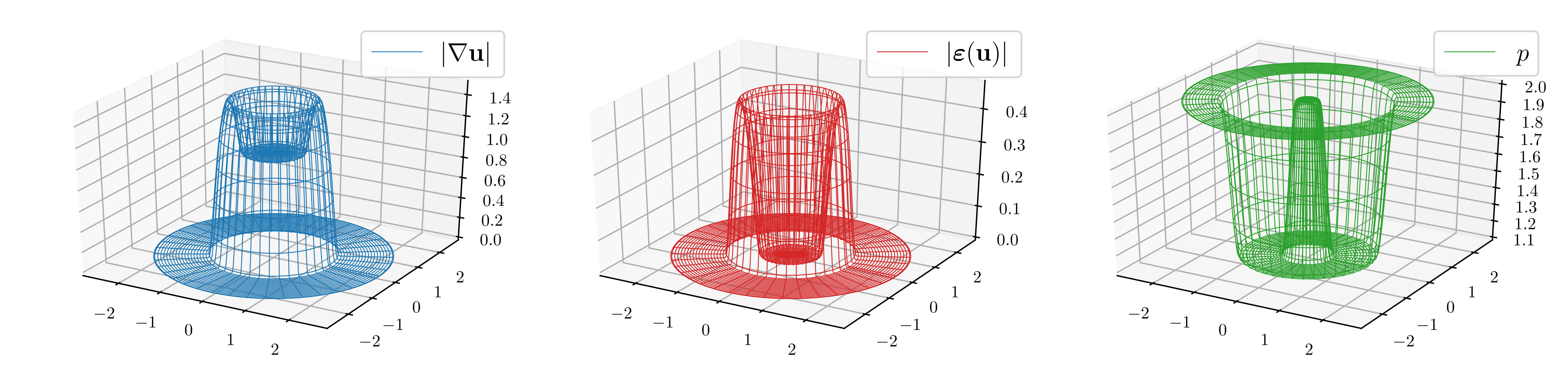
Figure 3: Plots of $|{\nabla}{\bf u}|\in C_{0}^{\infty}(\Omega)$ (blue/left), $|{\boldsymbol{\varepsilon}}({\bf u})|\in C_{0}^{\infty}(\Omega)$ (red/middle) and the exponent $p\in C^{\infty}(\mathbb{R}^{2})$ (green/right) constructed according to Proposition 4.4 for $d=2$, $\alpha=1.1$ and $\beta=2$.

In Figure 4 one can see for $I:=(-1.5,1.5)$, the function $\varphi\in L^{1.1}(I)\setminus L^{2}(I)$, given via ${\varphi(t):=\chi_{\left(-1,1\right)}(t)\big{(}|t|^{-\frac{1}{2}}-1\big{)}}$ for $t\in I$, and its approximations ${(\varphi_{n})_{n\in\mathbb{N}}:=(\varphi\ast\omega_{2^{-n}}^{1})_{n\in\mathbb{N}}\subseteq C_{0}^{\infty}(I)}$. According to Proposition 4.4, the sequence ${({\boldsymbol{\phi}}_{n})_{n\in\mathbb{N}}\subseteq C_{0}^{\infty}(Q_{T})^{d}}$, for every $(t,x)^{\top}\in Q_{T}$ and $n\in\mathbb{N}$ given via ${\boldsymbol{\phi}}_{n}(t,x):=\varphi_{n}(t){\bf u}(x)$, satisfies

$$\frac{\|{\nabla}{\boldsymbol{\phi}}_{n}\|_{L^{p(\cdot)}(Q_{T})^{d\times d}}}{\|{\boldsymbol{\varepsilon}}({\boldsymbol{\phi}}_{n})\|_{L^{p(\cdot)}(Q_{T})^{d\times d}}}\overset{n\to\infty}{\to}\infty.$$

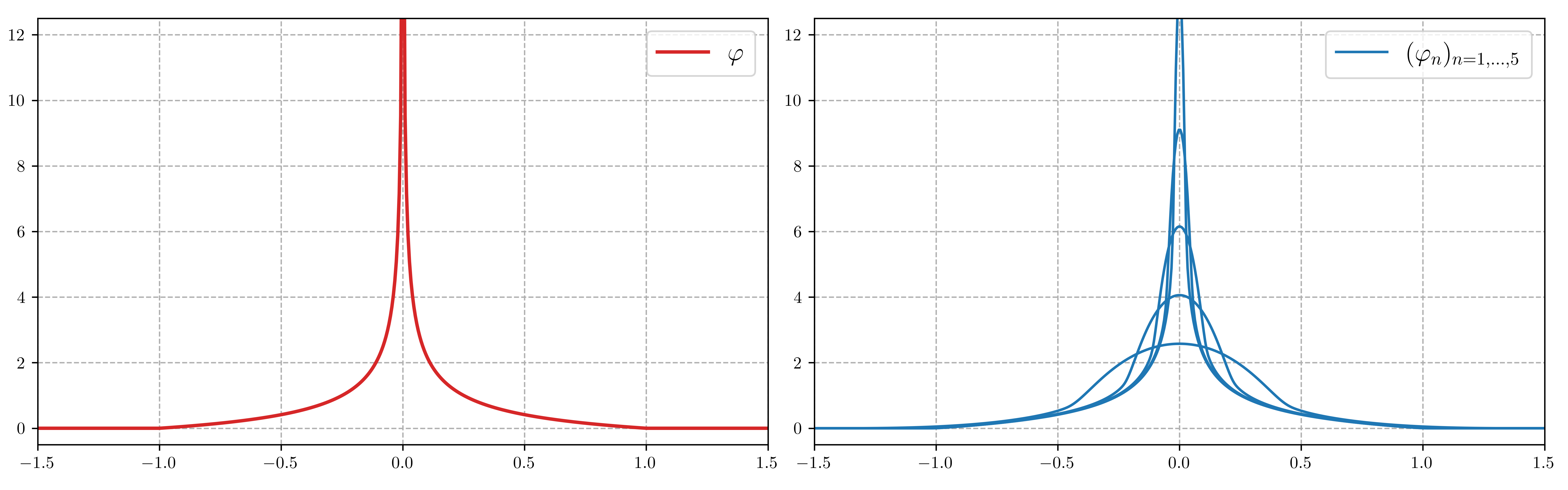
Figure 4: Plots of $\varphi\in L^{1.1}(I)\setminus L^{2}(I)$ (red/left) and $(\varphi_{n})_{n=1,...,5}\subseteq C_{0}^{\infty}(I)$ (blue/right).

In consequence, we have to distinguish between the spaces $\bscal{X}_{{\nabla}}^{q,p}(Q_{T})$ and $\bscal{X}_{{\boldsymbol{\varepsilon}}}^{q,p}(Q_{T})$, i.e., we have to equip $\bscal{X}_{{\nabla}}^{q,p}(Q_{T})$ and $\bscal{X}_{{\boldsymbol{\varepsilon}}}^{q,p}(Q_{T})$ with different norms, in order to guarantee at least the well-definedness of these norms.

Proposition 4.6

The spaces $\bscal{X}_{{\nabla}}^{q,p}(Q_{T})$ and $\bscal{X}_{{\boldsymbol{\varepsilon}}}^{q,p}(Q_{T})$ equipped with the norms

$$\|\cdot\|_{\bscal{X}_{{\nabla}}^{q,p}(Q_{T})} :=\|\cdot\|_{L^{q(\cdot,\cdot)}(Q_{T})^{d}}+\|{\nabla}\cdot\|_{L^{p(\cdot,\cdot)}(Q_{T})^{d\times d}},$$

$$\|\cdot\|_{\bscal{X}_{{\boldsymbol{\varepsilon}}}^{q,p}(Q_{T})} :=\|\cdot\|_{L^{q(\cdot,\cdot)}(Q_{T})^{d}}+\|{\boldsymbol{\varepsilon}}(\cdot)\|_{L^{p(\cdot,\cdot)}(Q_{T})^{d\times d}}$$

are Banach spaces. In addition, we have $\bscal{X}_{+}^{q,p}(Q_{T})\hookrightarrow\bscal{X}_{{\nabla}}^{q,p}(Q_{T})\hookrightarrow\bscal{X}_{{\boldsymbol{\varepsilon}}}^{q,p}(Q_{T})\hookrightarrow\bscal{X}_{-}^{q,p}(Q_{T})$.

Proof

We only give a proof for $\bscal{X}_{{\boldsymbol{\varepsilon}}}^{q,p}(Q_{T})$, since all arguments transfer to $\bscal{X}_{{\nabla}}^{q,p}(Q_{T})$.

The norm properties follow from the definition. Hence, it remains to prove completeness. To this end, let $({\boldsymbol{u}}_{n})_{n\in\mathbb{N}}\subseteq\bscal{X}_{{\boldsymbol{\varepsilon}}}^{q,p}(Q_{T})$ be a Cauchy sequence, i.e., also $({\boldsymbol{u}}_{n})_{n\in\mathbb{N}}\subseteq L^{q(\cdot,\cdot)}(Q_{T})^{d}$ and $({\boldsymbol{\varepsilon}}({\boldsymbol{u}}_{n}))_{n\in\mathbb{N}}\subseteq L^{p(\cdot,\cdot)}(Q_{T},\mathbb{M}^{d\times d}_{{\mathrm{sym}}})$ are Cauchy sequences. Thus, as $L^{q(\cdot,\cdot)}(Q_{T})^{d}$ and $L^{p(\cdot,\cdot)}(Q_{T},\mathbb{M}^{d\times d}_{{\mathrm{sym}}})$ are Banach spaces, there exist elements ${\boldsymbol{u}}\in L^{q(\cdot,\cdot)}(Q_{T})^{d}$ and $\bscal{E}\in L^{p(\cdot,\cdot)}(Q_{T},\mathbb{M}^{d\times d}_{{\mathrm{sym}}})$, such that

$$\begin{split}\begin{aligned} {\boldsymbol{u}}_{n}&\overset{n\to\infty}{\to}{\boldsymbol{u}}&&\quad\text{ in }L^{q(\cdot,\cdot)}(Q_{T})^{d},\\ {\boldsymbol{\varepsilon}}({\boldsymbol{u}}_{n})&\overset{n\to\infty}{\to}\bscal{E}&&\quad\text{ in }L^{p(\cdot,\cdot)}(Q_{T},\mathbb{M}^{d\times d}_{{\mathrm{sym}}}).\end{aligned}\end{split}$$ (4.7)

Since norm convergence implies modular convergence, we infer from (4.7)

$$\begin{split}\int_{I}\rho_{q(t,\cdot)}({\boldsymbol{u}}_{n}(t)-{\boldsymbol{u}}(t))&+\rho_{p(t,\cdot)}({\boldsymbol{\varepsilon}}({\boldsymbol{u}}_{n})(t)-\bscal{E}(t))\,dt\\ &=\rho_{q(\cdot,\cdot)}({\boldsymbol{u}}_{n}-{\boldsymbol{u}})+\rho_{p(\cdot,\cdot)}({\boldsymbol{\varepsilon}}({\boldsymbol{u}}_{n})-\bscal{E})\overset{n\to\infty}{\to}0.\end{split}$$ (4.8)

Thus, (4.8) yields a subsequence $({\boldsymbol{u}}_{n})_{n\in\Lambda}\subseteq\bscal{X}^{q,p}_{{\boldsymbol{\varepsilon}}}(Q_{T})$, with $\Lambda\subseteq\mathbb{N}$, such that for almost every ${t\in I}$

$$\rho_{q(t,\cdot)}({\boldsymbol{u}}_{n}(t)-{\boldsymbol{u}}(t))+\rho_{p(t,\cdot)}({\boldsymbol{\varepsilon}}({\boldsymbol{u}}_{n})(t)-\bscal{E}(t))\overset{n\to\infty}{\to}0\quad(n\in\Lambda).$$ (4.9)

As conversely modular convergence implies norm convergence, (4.9) yields for almost every ${t\in I}$

$$\begin{split}\begin{aligned} {\boldsymbol{u}}_{n}(t)&\overset{n\to\infty}{\to}{\boldsymbol{u}}(t)&&\quad\text{ in }L^{q(t,\cdot)}(\Omega)^{d}\quad\quad(n\in\Lambda),\\ {\boldsymbol{\varepsilon}}({\boldsymbol{u}}_{n})(t)&\overset{n\to\infty}{\to}\bscal{E}(t)&&\quad\text{ in }L^{p(t,\cdot)}(\Omega,\mathbb{M}^{d\times d}_{{\mathrm{sym}}})\quad(n\in\Lambda).\end{aligned}\end{split}$$ (4.10)

From (4.10) we derive that the sequence $({\boldsymbol{u}}_{n}(t))_{n\in\Lambda}\subseteq X^{q,p}_{{\boldsymbol{\varepsilon}}}(t)$ is for almost every $t\in I$ a Cauchy sequence. Since for almost every $t\in I$ the space $X^{q,p}_{{\boldsymbol{\varepsilon}}}(t)$ is a Banach space, we obtain for almost every $t\in I$ that ${\boldsymbol{u}}(t)\in X^{q,p}_{{\boldsymbol{\varepsilon}}}(t)$ with ${\boldsymbol{\varepsilon}}({\boldsymbol{u}})(t)=\bscal{E}(t)$ in $L^{p(t,\cdot)}(\Omega,\mathbb{M}^{d\times d}_{{\mathrm{sym}}})$ and ${\boldsymbol{u}}_{n}(t)\to{\boldsymbol{u}}(t)$ in $X^{q,p}_{{\boldsymbol{\varepsilon}}}(t)$ $(\Lambda\ni n\to\infty)$. In other words, we have ${\boldsymbol{u}}\in\bscal{X}^{q,p}_{{\boldsymbol{\varepsilon}}}(Q_{T})$ and ${\boldsymbol{u}}_{n}\to{\boldsymbol{u}}$ in $\bscal{X}^{q,p}_{{\boldsymbol{\varepsilon}}}(Q_{T})$ $(n\to\infty)$, i.e., $\bscal{X}^{q,p}_{{\boldsymbol{\varepsilon}}}(Q_{T})$ is complete.

The embedding $\bscal{X}_{+}^{q,p}(Q_{T})\hookrightarrow\bscal{X}_{{\nabla}}^{q,p}(Q_{T})$ follows from the embeddings $L^{q^{+}}(Q_{T})^{d}\hookrightarrow L^{q(\cdot,\cdot)}(Q_{T})^{d}$ and $L^{p^{+}}(Q_{T})^{d\times d}\hookrightarrow L^{p(\cdot,\cdot)}(Q_{T})^{d\times d}$ (cf. (DHHR11, , Theorem 3.3.1.)). The embedding $\bscal{X}_{{\nabla}}^{q,p}(Q_{T})\hookrightarrow\bscal{X}^{q,p}_{{\boldsymbol{\varepsilon}}}(Q_{T})$ is evident. The embedding $\bscal{X}^{q,p}_{{\boldsymbol{\varepsilon}}}(Q_{T})\hookrightarrow\bscal{X}_{-}^{q,p}(Q_{T})$ follows from the embeddings $L^{q(\cdot,\cdot)}(Q_{T})^{d}\hookrightarrow L^{q^{-}}(Q_{T})^{d}$ and $L^{p(\cdot,\cdot)}(Q_{T},\mathbb{M}^{d\times d}_{{\mathrm{sym}}})^{d}\hookrightarrow L^{p^{-}}(Q_{T},\mathbb{M}^{d\times d}_{{\mathrm{sym}}})^{d}$ as well as Korn’s inequality for the constant exponent $p^{-}\in\left(1,\infty\right)$. ∎

Henceforth, this article will primarily treat the space $\bscal{X}_{{\boldsymbol{\varepsilon}}}^{q,p}(Q_{T})$, as this space is of greater interest with regard to the model problem (1.1). However, we emphasize that all following definitions and results admit congruent adaptations to $\bscal{X}_{{\nabla}}^{q,p}(Q_{T})$.

Corollary 4.11

Let $({\boldsymbol{u}}_{n})_{n\in\mathbb{N}}\subseteq\bscal{X}^{q,p}_{{\boldsymbol{\varepsilon}}}(Q_{T})$ be a sequence, such that ${\boldsymbol{u}}_{n}\to{\boldsymbol{u}}\text{ in }\bscal{X}^{q,p}_{{\boldsymbol{\varepsilon}}}(Q_{T})$ ${(n\to\infty)}$. Then, there exists a subsequence $({\boldsymbol{u}}_{n})_{n\in\Lambda}\subseteq\bscal{X}^{q,p}_{{\boldsymbol{\varepsilon}}}(Q_{T})$, with $\Lambda\subseteq\mathbb{N}$, such that ${\boldsymbol{u}}_{n}(t)\to{\boldsymbol{u}}(t)$ in $X^{q,p}_{{\boldsymbol{\varepsilon}}}(t)$ $(\Lambda\ni n\to\infty)$ for almost every $t\in I$.

Proposition 4.12

The mapping ${\boldsymbol{\Pi}}_{{\boldsymbol{\varepsilon}}}:\bscal{X}^{q,p}_{{\boldsymbol{\varepsilon}}}(Q_{T})\to L^{q(\cdot,\cdot)}(Q_{T})^{d}\times L^{p(\cdot,\cdot)}(Q_{T},\mathbb{M}_{{\mathrm{sym}}}^{d\times d})$, given via

$${\boldsymbol{\Pi}}_{{\boldsymbol{\varepsilon}}}{\boldsymbol{u}}:=({\boldsymbol{u}},{\boldsymbol{\varepsilon}}({\boldsymbol{u}}))^{\top}\quad\text{ in }L^{q(\cdot,\cdot)}(Q_{T})^{d}\times L^{p(\cdot,\cdot)}(Q_{T},\mathbb{M}_{{\mathrm{sym}}}^{d\times d})$$

for every ${\boldsymbol{u}}\in\bscal{X}^{q,p}_{{\boldsymbol{\varepsilon}}}(Q_{T})$, is an isometric isomorphism into its range $R({\boldsymbol{\Pi}}_{{\boldsymbol{\varepsilon}}})$. In particular, $\bscal{X}_{{\boldsymbol{\varepsilon}}}^{q,p}(Q_{T})$ is separable. In addition, if $q^{-},p^{-}>1$, then $\bscal{X}_{{\boldsymbol{\varepsilon}}}^{q,p}(Q_{T})$ is reflexive.

Proof

Since ${\boldsymbol{\Pi}}_{{\boldsymbol{\varepsilon}}}:\bscal{X}_{{\boldsymbol{\varepsilon}}}^{q,p}(Q_{T})\to L^{q(\cdot,\cdot)}(Q_{T})^{d}\times L^{p(\cdot,\cdot)}(Q_{T},\mathbb{M}_{{\mathrm{sym}}}^{d\times d})$ is an isometry and $\bscal{X}_{{\boldsymbol{\varepsilon}}}^{q,p}(Q_{T})$ a Banach space (cf. Proposition 4.6), $R({\boldsymbol{\Pi}}_{{\boldsymbol{\varepsilon}}})$ is a closed subspace of ${L^{q(\cdot,\cdot)}(Q_{T})^{d}\times L^{p(\cdot,\cdot)}(Q_{T},\mathbb{M}_{\textup{sym}}^{d\times d})}$, i.e., $R({\boldsymbol{\Pi}}_{{\boldsymbol{\varepsilon}}})$ is a Banach space, and therefore ${\boldsymbol{\Pi}}_{{\boldsymbol{\varepsilon}}}:\bscal{X}_{{\boldsymbol{\varepsilon}}}^{q,p}(Q_{T})\to R({\boldsymbol{\Pi}}_{{\boldsymbol{\varepsilon}}})$ an isometric isomorphism. As $L^{q(\cdot,\cdot)}(Q_{T})^{d}$ and $L^{p(\cdot,\cdot)}(Q_{T},\mathbb{M}_{{\mathrm{sym}}}^{d\times d})$ are separable, the product ${L^{q(\cdot,\cdot)}(Q_{T})^{d}\times L^{p(\cdot,\cdot)}(Q_{T},\mathbb{M}_{{\mathrm{sym}}}^{d\times d})}$ is separable as well. Thus, $R({\boldsymbol{\Pi}}_{{\boldsymbol{\varepsilon}}})$ inherits the separability of ${L^{q(\cdot,\cdot)}(Q_{T})^{d}\times L^{p(\cdot,\cdot)}(Q_{T},\mathbb{M}_{{\mathrm{sym}}}^{d\times d})}$, and in virtue of the isomorphism ${\boldsymbol{\Pi}}_{{\boldsymbol{\varepsilon}}}:\bscal{X}_{{\boldsymbol{\varepsilon}}}^{q,p}(Q_{T})\to R({\boldsymbol{\Pi}}_{{\boldsymbol{\varepsilon}}})$ also $\bscal{X}_{{\boldsymbol{\varepsilon}}}^{q,p}(Q_{T})$. If additionally $q^{-},p^{-}>1$, then the spaces $L^{q(\cdot,\cdot)}(Q_{T})^{d}$ and $L^{p(\cdot,\cdot)}(Q_{T},\mathbb{M}_{{\mathrm{sym}}}^{d\times d})$, and thus also the product $L^{q(\cdot,\cdot)}(Q_{T})^{d}\times L^{p(\cdot,\cdot)}(Q_{T},\mathbb{M}_{{\mathrm{sym}}}^{d\times d})$, are reflexive (cf. Proposition 2.11). Hence, the range $R({\boldsymbol{\Pi}}_{{\boldsymbol{\varepsilon}}})$ is reflexive and, in virtue of the isomorphism ${{\boldsymbol{\Pi}}_{{\boldsymbol{\varepsilon}}}:\bscal{X}_{{\boldsymbol{\varepsilon}}}^{q,p}(Q_{T})\to R({\boldsymbol{\Pi}}_{{\boldsymbol{\varepsilon}}})}$, also $\bscal{X}_{{\boldsymbol{\varepsilon}}}^{q,p}(Q_{T})$.  ∎

Proposition 4.13 (Characterization of $\bscal{X}^{q,p}_{{\boldsymbol{\varepsilon}}}(Q_{T})^{*}$)

Let $q^{-},p^{-}>1$. Then, the operator $\bscal{J}_{{\boldsymbol{\varepsilon}}}:L^{q^{\prime}(\cdot,\cdot)}(Q_{T})^{d}\times L^{p^{\prime}(\cdot,\cdot)}(Q_{T},\mathbb{M}_{{\mathrm{sym}}}^{d\times d})\to\bscal{X}^{q,p}_{{\boldsymbol{\varepsilon}}}(Q_{T})^{*}$, given via

$$\langle\bscal{J}_{{\boldsymbol{\varepsilon}}}({\boldsymbol{f}},{\boldsymbol{F}}),{\boldsymbol{u}}\rangle_{\bscal{X}^{q,p}_{{\boldsymbol{\varepsilon}}}(Q_{T})} :=({\boldsymbol{f}},{\boldsymbol{u}})_{L^{q(\cdot,\cdot)}(Q_{T})^{d}}+({\boldsymbol{F}},{\boldsymbol{\varepsilon}}({\boldsymbol{u}}))_{L^{p(\cdot,\cdot)}(Q_{T})^{d\times d}}$$

for every ${\boldsymbol{f}}\in L^{q^{\prime}(\cdot,\cdot)}(Q_{T})^{d}$, ${\boldsymbol{F}}\in L^{p^{\prime}(\cdot,\cdot)}(Q_{T},\mathbb{M}_{{\mathrm{sym}}}^{d\times d})$ and ${\boldsymbol{u}}\in\bscal{X}^{q,p}_{{\boldsymbol{\varepsilon}}}(Q_{T})$, is well-defined, linear and Lipschitz continuous with constant $2$. In addition, for every ${\boldsymbol{u}}^{*}\in\bscal{X}^{q,p}_{{\boldsymbol{\varepsilon}}}(Q_{T})^{*}$ there exist ${\boldsymbol{f}}\in L^{q^{\prime}(\cdot,\cdot)}(Q_{T})^{d}$, ${\boldsymbol{F}}\in L^{p^{\prime}(\cdot,\cdot)}(Q_{T},\mathbb{M}_{{\mathrm{sym}}}^{d\times d})$, such that ${\boldsymbol{u}}^{*}=\bscal{J}_{{\boldsymbol{\varepsilon}}}({\boldsymbol{f}},{\boldsymbol{F}})$ in $\bscal{X}^{q,p}_{{\boldsymbol{\varepsilon}}}(Q_{T})^{*}$ and

$$\frac{1}{2}\|{\boldsymbol{u}}^{*}\|_{\bscal{X}^{q,p}_{{\boldsymbol{\varepsilon}}}(Q_{T})^{*}}\leq\|{\boldsymbol{f}}\|_{L^{q^{\prime}(\cdot,\cdot)}(Q_{T})^{d}}+\|{\boldsymbol{F}}\|_{L^{p^{\prime}(\cdot,\cdot)}(Q_{T})^{d\times d}}\leq 2\|{\boldsymbol{u}}^{*}\|_{\bscal{X}^{q,p}_{{\boldsymbol{\varepsilon}}}(Q_{T})^{*}}.$$ (4.14)

Remark 4.15

The operator $\bscal{J}_{{\boldsymbol{\varepsilon}}}:L^{q^{\prime}(\cdot,\cdot)}(Q_{T})^{d}\times L^{p^{\prime}(\cdot,\cdot)}(Q_{T},\mathbb{M}_{{\mathrm{sym}}}^{d\times d})\to\bscal{X}^{q,p}_{{\boldsymbol{\varepsilon}}}(Q_{T})^{*}$ is closely related to the adjoint operator ${\boldsymbol{\Pi}}_{{\boldsymbol{\varepsilon}}}^{*}:(L^{q(\cdot,\cdot)}(Q_{T})^{d}\times L^{p(\cdot,\cdot)}(Q_{T},\mathbb{M}_{{\mathrm{sym}}}^{d\times d}))^{*}\to\bscal{X}^{q,p}_{{\boldsymbol{\varepsilon}}}(Q_{T})^{*}$. In fact, consider ${\boldsymbol{J}}_{q,p}:L^{q^{\prime}(\cdot,\cdot)}(Q_{T})^{d}\times L^{p^{\prime}(\cdot,\cdot)}(Q_{T},\mathbb{M}_{{\mathrm{sym}}}^{d\times d})\to(L^{q(\cdot,\cdot)}(Q_{T})^{d}\times L^{p(\cdot,\cdot)}(Q_{T},\mathbb{M}_{{\mathrm{sym}}}^{d\times d}))^{*}$, given via

$$\langle{\boldsymbol{J}}_{q,p}({\boldsymbol{f}},{\boldsymbol{F}}),({\boldsymbol{g}},{\boldsymbol{G}})^{\top}\rangle_{L^{q(\cdot,\cdot)}(Q_{T})^{d}\times L^{p(\cdot,\cdot)}(Q_{T},\mathbb{M}_{{\mathrm{sym}}}^{d\times d})}:=({\boldsymbol{f}},{\boldsymbol{g}})_{L^{q(\cdot,\cdot)}(Q_{T})^{d}}+({\boldsymbol{F}},{\boldsymbol{G}})_{L^{p(\cdot,\cdot)}(Q_{T})^{d\times d}}$$

for every ${\boldsymbol{f}}\in L^{q^{\prime}(\cdot,\cdot)}(Q_{T})^{d}$, ${\boldsymbol{g}}\in L^{q(\cdot,\cdot)}(Q_{T})^{d}$, ${\boldsymbol{F}}\in L^{p^{\prime}(\cdot,\cdot)}(Q_{T},\mathbb{M}_{{\mathrm{sym}}}^{d\times d})$ and ${\boldsymbol{G}}\in L^{p(\cdot,\cdot)}(Q_{T},\mathbb{M}_{{\mathrm{sym}}}^{d\times d})$. Using Proposition 2.11, we deduce for every ${\boldsymbol{f}}\in L^{q^{\prime}(\cdot,\cdot)}(Q_{T})^{d}$ and ${\boldsymbol{F}}\in L^{p^{\prime}(\cdot,\cdot)}(Q_{T},\mathbb{M}_{{\mathrm{sym}}}^{d\times d})$ that

$$\begin{split}\frac{1}{2}\|({\boldsymbol{f}},{\boldsymbol{F}})^{\top}\|_{L^{q^{\prime}(\cdot,\cdot)}(Q_{T})^{d}\times L^{p^{\prime}(\cdot,\cdot)}(Q_{T})^{d\times d}}&\leq\|{\boldsymbol{J}}_{q,p}({\boldsymbol{f}},{\boldsymbol{F}})\|_{(L^{q(\cdot,\cdot)}(Q_{T})^{d}\times L^{p(\cdot,\cdot)}(Q_{T},\mathbb{M}_{{\mathrm{sym}}}^{d\times d}))^{*}}\\ &\leq 2\|({\boldsymbol{f}},{\boldsymbol{F}})^{\top}\|_{L^{q^{\prime}(\cdot,\cdot)}(Q_{T})^{d}\times L^{p^{\prime}(\cdot,\cdot)}(Q_{T})^{d\times d}},\end{split}$$ (4.16)

i.e., ${\boldsymbol{J}}_{q,p}:L^{q^{\prime}(\cdot,\cdot)}(Q_{T})^{d}\times L^{p^{\prime}(\cdot,\cdot)}(Q_{T},\mathbb{M}_{{\mathrm{sym}}}^{d\times d})\to(L^{q(\cdot,\cdot)}(Q_{T})^{d}\times L^{p(\cdot,\cdot)}(Q_{T},\mathbb{M}_{{\mathrm{sym}}}^{d\times d}))^{*}$ is an isomorphism. Moreover, we have $\bscal{J}_{{\boldsymbol{\varepsilon}}}={\boldsymbol{\Pi}}_{{\boldsymbol{\varepsilon}}}^{*}\circ{\boldsymbol{J}}_{q,p}$, i.e., $\bscal{J}_{{\boldsymbol{\varepsilon}}}$ and ${\boldsymbol{\Pi}}_{{\boldsymbol{\varepsilon}}}^{*}$ coincide up to the isomorphism ${\boldsymbol{J}}_{q,p}$.

Proof

(of Proposition 4.13) Well-definedness, linearity and Lipschitz continuity with constant $2$ follow from Hölder’s inequality. So, let us prove the surjectivity including (4.14). For ${{\boldsymbol{u}}^{*}\in\bscal{X}^{q,p}_{{\boldsymbol{\varepsilon}}}(Q_{T})^{*}}$ we define $\widetilde{\boldsymbol{u}}\in(R({\boldsymbol{\Pi}}_{{\boldsymbol{\varepsilon}}}))^{*}$ via $\langle\widetilde{\boldsymbol{u}},{\boldsymbol{\Pi}}_{{\boldsymbol{\varepsilon}}}{\boldsymbol{u}}\rangle_{R({\boldsymbol{\Pi}}_{{\boldsymbol{\varepsilon}}})}:=\langle{\boldsymbol{u}}^{*},{\boldsymbol{u}}\rangle_{\bscal{X}^{q,p}_{{\boldsymbol{\varepsilon}}}(Q_{T})}$ for every ${\boldsymbol{u}}\in\bscal{X}^{q,p}_{{\boldsymbol{\varepsilon}}}(Q_{T})$. Since ${\boldsymbol{\Pi}}_{{\boldsymbol{\varepsilon}}}$ is an isometric isomorphism, we have ${\lVert{\widetilde{\boldsymbol{u}}}\rVert}_{(R({\boldsymbol{\Pi}}_{{\boldsymbol{\varepsilon}}}))^{*}}={\lVert{{\boldsymbol{u}}^{*}}\rVert}_{\bscal{X}^{q,p}_{{\boldsymbol{\varepsilon}}}(Q_{T})^{*}}$. The Hahn–Banach theorem yields a norm preserving extension $\widehat{\boldsymbol{u}}\in(L^{q(\cdot,\cdot)}(Q_{T})^{d}\times L^{p(\cdot,\cdot)}(Q_{T},\mathbb{M}_{{\mathrm{sym}}}^{d\times d}))^{*}$ of $\widetilde{\boldsymbol{u}}\in(R({\boldsymbol{\Pi}}_{{\boldsymbol{\varepsilon}}}))^{*}$. From Remark 4.15 follows that there exist functions ${\boldsymbol{f}}\in L^{q^{\prime}(\cdot,\cdot)}(Q_{T})^{d}$ and ${\boldsymbol{F}}\in L^{p^{\prime}(\cdot,\cdot)}(Q_{T},\mathbb{M}_{{\mathrm{sym}}}^{d\times d})$, such that ${\boldsymbol{J}}_{q,p}({\boldsymbol{f}},{\boldsymbol{F}})=\widehat{\boldsymbol{u}}$ in $(L^{q(\cdot,\cdot)}(Q_{T})^{d}\times L^{p(\cdot,\cdot)}(Q_{T},\mathbb{M}_{{\mathrm{sym}}}^{d\times d}))^{*}$. Consequently, there holds for every ${\boldsymbol{u}}\in\bscal{X}^{q,p}_{{\boldsymbol{\varepsilon}}}(Q_{T})$

$$\langle{\boldsymbol{u}}^{*},{\boldsymbol{u}}\rangle_{\bscal{X}^{q,p}_{{\boldsymbol{\varepsilon}}}(Q_{T})} =\langle\widetilde{\boldsymbol{u}},{\boldsymbol{\Pi}}_{{\boldsymbol{\varepsilon}}}{\boldsymbol{u}}\rangle_{R({\boldsymbol{\Pi}}_{{\boldsymbol{\varepsilon}}})}$$

$$=\langle\widehat{\boldsymbol{u}},{\boldsymbol{\Pi}}_{{\boldsymbol{\varepsilon}}}{\boldsymbol{u}}\rangle_{L^{q(\cdot,\cdot)}(Q_{T})^{d}\times L^{p(\cdot,\cdot)}(Q_{T},\mathbb{M}_{{\mathrm{sym}}}^{d\times d})}$$

$$=\langle{\boldsymbol{J}}_{q,p}({\boldsymbol{f}},{\boldsymbol{F}}),{\boldsymbol{\Pi}}_{{\boldsymbol{\varepsilon}}}{\boldsymbol{u}}\rangle_{L^{q(\cdot,\cdot)}(Q_{T})^{d}\times L^{p(\cdot,\cdot)}(Q_{T},\mathbb{M}_{{\mathrm{sym}}}^{d\times d})}$$

$$=({\boldsymbol{f}},{\boldsymbol{u}})_{L^{q(\cdot,\cdot)}(Q_{T})^{d}}+({\boldsymbol{F}},{\boldsymbol{\varepsilon}}({\boldsymbol{u}}))_{L^{p(\cdot,\cdot)}(Q_{T})^{d\times d}}$$

$$=\langle\bscal{J}_{{\boldsymbol{\varepsilon}}}({\boldsymbol{f}},{\boldsymbol{F}}),{\boldsymbol{u}}\rangle_{\bscal{X}^{q,p}_{{\boldsymbol{\varepsilon}}}(Q_{T})},$$

i.e., ${\boldsymbol{u}}^{*}=\bscal{J}_{{\boldsymbol{\varepsilon}}}({\boldsymbol{f}},{\boldsymbol{F}})$ in $\bscal{X}^{q,p}_{{\boldsymbol{\varepsilon}}}(Q_{T})^{*}$. Thus, ${\bscal{J}_{{\boldsymbol{\varepsilon}}}:L^{q^{\prime}(\cdot,\cdot)}(Q_{T})^{d}\times L^{p^{\prime}(\cdot,\cdot)}(Q_{T},\mathbb{M}_{{\mathrm{sym}}}^{d\times d})\to\bscal{X}^{q,p}_{{\boldsymbol{\varepsilon}}}(Q_{T})^{*}}$ is surjective. In addition, from the above follows that ${\lVert{{\boldsymbol{u}}^{*}}\rVert}_{\bscal{X}^{q,p}_{{\boldsymbol{\varepsilon}}}(Q_{T})^{*}}={\lVert{\widetilde{\boldsymbol{u}}}\rVert}_{(R({\boldsymbol{\Pi}}_{{\boldsymbol{\varepsilon}}}))^{*}}=$ ${\lVert{\widehat{\boldsymbol{u}}}\rVert}_{(L^{q(\cdot,\cdot)}(Q_{T})^{d}\times L^{p(\cdot,\cdot)}(Q_{T},\mathbb{M}_{{\mathrm{sym}}}^{d\times d}))^{*}}={\lVert{{\boldsymbol{J}}_{q,p}({\boldsymbol{f}},{\boldsymbol{F}})}\rVert}_{(L^{q(\cdot,\cdot)}(Q_{T})^{d}\times L^{p(\cdot,\cdot)}(Q_{T},\mathbb{M}_{{\mathrm{sym}}}^{d\times d}))^{*}}$ and (4.14) follows from (4.16). ∎

In the same manner, we can characterize the dual space of $X_{{\boldsymbol{\varepsilon}}}^{q,p}=X^{q(\cdot),p(\cdot)}_{{\boldsymbol{\varepsilon}}}(\Omega)$.

Corollary 4.17

Let $q,p\in\mathcal{P}^{\infty}(\Omega)$. Then, the mapping ${\Pi_{{\boldsymbol{\varepsilon}}}:X_{{\boldsymbol{\varepsilon}}}^{q,p}\to L^{q(\cdot)}(\Omega)^{d}\times L^{p(\cdot)}(\Omega,\mathbb{M}^{d\times d}_{{\mathrm{sym}}})}$, for every ${\bf u}\in X_{{\boldsymbol{\varepsilon}}}^{q,p}$ given via

$$\Pi_{{\boldsymbol{\varepsilon}}}{\bf u}:=({\bf u},{\boldsymbol{\varepsilon}}({\bf u}))^{\top}\quad\textup{ in }L^{q(\cdot)}(\Omega)^{d}\times L^{p(\cdot)}(\Omega,\mathbb{M}^{d\times d}_{{\mathrm{sym}}}),$$

is an isometric isomorphism. In particular, $X_{{\boldsymbol{\varepsilon}}}^{q,p}$ is separable. Furthermore, if $q^{-},p^{-}>1$, then $X_{{\boldsymbol{\varepsilon}}}^{q,p}$ is reflexive and the operator $\mathcal{J}_{{\boldsymbol{\varepsilon}}}:L^{q^{\prime}(\cdot)}(\Omega)^{d}\times L^{p^{\prime}(\cdot)}(\Omega,\mathbb{M}^{d\times d}_{{\mathrm{sym}}})\to(X_{{\boldsymbol{\varepsilon}}}^{q,p})^{*}$, for every ${{\bf f}\in L^{q^{\prime}(\cdot)}(\Omega)^{d}}$, ${\bf F}\in L^{p^{\prime}(\cdot)}(\Omega,\mathbb{M}^{d\times d}_{{\mathrm{sym}}})$ and ${\bf u}\in X_{{\boldsymbol{\varepsilon}}}^{q,p}$ given via

$$\langle\mathcal{J}_{{\boldsymbol{\varepsilon}}}({\bf f},{\bf F}),{\bf u}\rangle_{X_{{\boldsymbol{\varepsilon}}}^{q,p}}=({\bf f},{\bf u})_{L^{q(\cdot)}(\Omega)^{d}}+({\bf F},{\boldsymbol{\varepsilon}}({\bf u}))_{L^{p(\cdot)}(\Omega)^{d\times d}}$$

is well-defined, linear and Lipschitz continuous with constant $2$. In additon, for every ${{\bf u}^{*}\in(X_{{\boldsymbol{\varepsilon}}}^{q,p})^{*}}$ there exist ${\bf f}\in L^{q^{\prime}(\cdot)}(\Omega)^{d}$ and ${\bf F}\in L^{p^{\prime}(\cdot)}(\Omega,\mathbb{M}^{d\times d}_{{\mathrm{sym}}})$, such that ${\bf u}^{*}=\mathcal{J}_{{\boldsymbol{\varepsilon}}}({\bf f},{\bf F})$ in $(X_{{\boldsymbol{\varepsilon}}}^{q,p})^{*}$ and

$$\frac{1}{2}\|{\bf u}^{*}\|_{(X_{{\boldsymbol{\varepsilon}}}^{q,p})^{*}}\leq\|{\bf f}\|_{L^{q^{\prime}(\cdot)}(\Omega)^{d}}+\|{\bf F}\|_{L^{p^{\prime}(\cdot)}(\Omega)^{d\times d}}\leq 2\|{\bf u}^{*}\|_{(X_{{\boldsymbol{\varepsilon}}}^{q,p})^{*}}.$$

The following remark deals with the question of a well-posed definition of a time evaluation of functionals in $\bscal{X}^{q,p}_{{\boldsymbol{\varepsilon}}}(Q_{T})^{*}$.

Remark 4.18 (Time slices of functionals ${\boldsymbol{u}}^{*}\in\bscal{X}^{q,p}_{{\boldsymbol{\varepsilon}}}(Q_{T})^{*}$)

Let $q^{-},p^{-}>1$.

(i)

Since for functions ${\boldsymbol{f}}\in L^{q^{\prime}(\cdot,\cdot)}(Q_{T})^{d}$ and ${\boldsymbol{F}}\in L^{p^{\prime}(\cdot,\cdot)}(Q_{T},\mathbb{M}_{{\mathrm{sym}}}^{d\times d})$ it holds ${\boldsymbol{f}}(t)\in L^{q^{\prime}(t,\cdot)}(\Omega)^{d}$ and ${\boldsymbol{F}}(t)\in L^{p^{\prime}(t,\cdot)}(\Omega,\mathbb{M}_{{\mathrm{sym}}}^{d\times d})$ for almost every $t\in I$ by Fubini’s theorem, Corollary 4.17 yields $\mathcal{J}_{{\boldsymbol{\varepsilon}}}({\boldsymbol{f}}(t),{\boldsymbol{F}}(t))\in X^{q,p}_{{\boldsymbol{\varepsilon}}}(t)^{*}$ for almost every $t\in I$. Fubini’s theorem also implies, due to Hölder’s inequality, for every ${\boldsymbol{u}}\in\bscal{X}^{q,p}_{{\boldsymbol{\varepsilon}}}(Q_{T})$, i.e., ${\boldsymbol{u}}(t)\in X^{q,p}_{{\boldsymbol{\varepsilon}}}(t)$ for almost every $t\in I$, that $(t\mapsto\langle\mathcal{J}_{{\boldsymbol{\varepsilon}}}({\boldsymbol{f}}(t),{\boldsymbol{F}}(t)),{\boldsymbol{u}}(t)\rangle_{X^{q,p}_{{\boldsymbol{\varepsilon}}}(t)})=(t\mapsto({\boldsymbol{f}}(t),{\boldsymbol{u}}(t))_{L^{q(t,\cdot)}(\Omega)^{d}}+({\boldsymbol{F}}(t),{\boldsymbol{\varepsilon}}({\boldsymbol{u}}(t)))_{L^{p(t,\cdot)}(\Omega)^{d\times d}})$ belongs to $L^{1}(I)$. More precisely, we have

$$\begin{split}\langle\bscal{J}_{{\boldsymbol{\varepsilon}}}({\boldsymbol{f}},{\boldsymbol{F}}),{\boldsymbol{u}}\rangle_{\bscal{X}^{q,p}_{{\boldsymbol{\varepsilon}}}(Q_{T})}&=\int_{I}{({\boldsymbol{f}}(t),{\boldsymbol{u}}(t))_{L^{q(t,\cdot)}(\Omega)^{d}}+({\boldsymbol{F}}(t),{\boldsymbol{\varepsilon}}({\boldsymbol{u}}(t)))_{L^{p(t,\cdot)}(\Omega)^{d\times d}}\,dt}\\ &=\int_{I}{\langle\mathcal{J}_{{\boldsymbol{\varepsilon}}}({\boldsymbol{f}}(t),{\boldsymbol{F}}(t)),{\boldsymbol{u}}(t)\rangle_{X^{q,p}_{{\boldsymbol{\varepsilon}}}(t)}\,dt}.\end{split}$$ (4.19)

(ii)

At first sight, it is not clear, whether ${\boldsymbol{u}}^{*}\in\bscal{X}^{q,p}_{{\boldsymbol{\varepsilon}}}(Q_{T})^{*}$ possesses time slices, in the sense that ${\boldsymbol{u}}^{*}(t)\in X^{q,p}_{{\boldsymbol{\varepsilon}}}(t)^{*}$ for almost every $t\in I$. But since due to Proposition 4.13 there exist ${\boldsymbol{f}}\in L^{q^{\prime}(\cdot,\cdot)}(Q_{T})^{d}$ and ${\boldsymbol{F}}\in L^{p^{\prime}(\cdot,\cdot)}(Q_{T},\mathbb{M}_{{\mathrm{sym}}}^{d\times d})$, such that ${\boldsymbol{u}}^{*}=\bscal{J}_{{\boldsymbol{\varepsilon}}}({\boldsymbol{f}},{\boldsymbol{F}})$ in $\bscal{X}^{q,p}_{{\boldsymbol{\varepsilon}}}(Q_{T})^{*}$, we are apt to define

$${\boldsymbol{u}}^{*}(t):=\mathcal{J}_{{\boldsymbol{\varepsilon}}}({\boldsymbol{f}}(t),{\boldsymbol{F}}(t))\quad\textup{ in }X^{q,p}_{{\boldsymbol{\varepsilon}}}(t)^{*}\quad\text{ for a.e. }t\in I.$$ (4.20)

To this end, we have to clarify, whether (4.20) is well-defined, i.e., independent of the choice of ${\boldsymbol{f}}\in L^{q^{\prime}(\cdot,\cdot)}(Q_{T})^{d}$ and ${\boldsymbol{F}}\in L^{p^{\prime}(\cdot,\cdot)}(Q_{T},\mathbb{M}_{{\mathrm{sym}}}^{d\times d})$. So, let us consider a further representation ${\boldsymbol{g}}\in L^{q^{\prime}(\cdot,\cdot)}(Q_{T})^{d}$ and ${\boldsymbol{G}}\in L^{p^{\prime}(\cdot,\cdot)}(Q_{T},\mathbb{M}_{{\mathrm{sym}}}^{d\times d})$, such that ${\boldsymbol{u}}^{*}=\bscal{J}_{{\boldsymbol{\varepsilon}}}({\boldsymbol{g}},{\boldsymbol{G}})$ in $\bscal{X}^{q,p}_{{\boldsymbol{\varepsilon}}}(Q_{T})^{*}$. Thus, testing by ${\boldsymbol{u}}:={\bf u}\varphi\in\bscal{X}^{q,p}_{{\boldsymbol{\varepsilon}}}(Q_{T})$, where ${\bf u}\in X_{+}^{q,p}$ and $\varphi\in C^{\infty}(I)$ are arbitrary, also using (4.19), we obtain

$$\int_{I}{\langle\mathcal{J}_{{\boldsymbol{\varepsilon}}}({\boldsymbol{f}}(t),{\boldsymbol{F}}(t)),{\bf u}\rangle_{X^{q,p}_{{\boldsymbol{\varepsilon}}}(t)}\varphi(t)\,dt}=\int_{I}{\langle\mathcal{J}_{{\boldsymbol{\varepsilon}}}({\boldsymbol{g}}(t),{\boldsymbol{G}}(t)),{\bf u}\rangle_{X^{q,p}_{{\boldsymbol{\varepsilon}}}(t)}\varphi(t)\,dt},$$

i.e., $\langle\mathcal{J}_{{\boldsymbol{\varepsilon}}}({\boldsymbol{f}}(t),{\boldsymbol{F}}(t)),{\bf u}\rangle_{X^{q,p}_{{\boldsymbol{\varepsilon}}}(t)}=\langle\mathcal{J}_{{\boldsymbol{\varepsilon}}}({\boldsymbol{g}}(t),{\boldsymbol{G}}(t)),{\bf u}\rangle_{X^{q,p}_{{\boldsymbol{\varepsilon}}}(t)}$ for almost every $t\in I$. Since $X_{+}^{q,p}$ is for almost every $t\in I$ dense in $X^{q,p}_{{\boldsymbol{\varepsilon}}}(t)$, we conclude $\mathcal{J}_{{\boldsymbol{\varepsilon}}}({\boldsymbol{f}}(t),{\boldsymbol{F}}(t))=\mathcal{J}_{{\boldsymbol{\varepsilon}}}({\boldsymbol{g}}(t),{\boldsymbol{G}}(t))$ in $X^{q,p}_{{\boldsymbol{\varepsilon}}}(t)^{*}$ for almost every $t\in I$. Therefore, the time slices (4.20) are well-defined.

5 Smoothing in $\bscal{X}^{q,p}_{{\boldsymbol{\varepsilon}}}(Q_{T})$ and $\bscal{X}^{q,p}_{{\boldsymbol{\varepsilon}}}(Q_{T})^{*}$

This section is concerned with the construction of an appropriate smoothing operator for $\bscal{X}^{q,p}_{{\boldsymbol{\varepsilon}}}(Q_{T})$ and $\bscal{X}^{q,p}_{{\boldsymbol{\varepsilon}}}(Q_{T})^{*}$. We emphasize that the presented smoothing method is not new and is based on ideas from DNR12 . However, in DNR12 it is solely shown that the smoothing method applies to $\bscal{X}^{q,p}_{{\nabla}}(Q_{T})$. An essential component of the argumentation was the pointwise Poincaré inequality (1.4). We extend the method to the greater space $\bscal{X}^{q,p}_{{\boldsymbol{\varepsilon}}}(Q_{T})$, by means of the pointwise Poincaré inequality for the symmetric gradient near the boundary of a bounded Lipschitz domain (cf. Theorem 3.1).

In what follows, let $\Omega\subseteq\mathbb{R}^{d}$, $d\geq 2$, be a bounded Lipschitz domain, $I=\left(0,T\right)$, with ${0<T<\infty}$, $Q_{T}=I\times\Omega$ and $q,p\in\mathcal{P}^{\log}(Q_{T})$ with $q^{-},p^{-}>1$.

For the constants $c_{0},h_{0}>0$, provided by Theorem 3.1, we set $h_{1}:=\frac{h_{0}}{4}$ and $(\eta_{h})_{h>0}:=(\omega_{h/2}^{d}\ast\chi_{\Omega_{5/2h}})_{h>0}\subseteq C^{\infty}_{0}(\Omega)$. Thus, for every $h>0$ holds $\text{supp}(\eta_{h})\subset\Omega_{2h}$, $0\leq\eta_{h}\leq 1\text{ in }\Omega$, $\eta_{h}=1\text{ in }\Omega_{3h}$ and $\|{\nabla}\eta_{h}\|_{L^{\infty}(\mathbb{R}^{d})^{d}}\leq\frac{c_{\eta}}{h}$, where $c_{\eta}>0$ is a constant not depending on $h>0$. Henceforth, we will always denote by ${\boldsymbol{\omega}}:=\omega^{d+1}\in C_{0}^{\infty}(B_{1}^{d+1}(0))$ the standard mollifier from Proposition 2.17. Likewise we define the family of scaled mollifiers ${\boldsymbol{\omega}}_{h}\in C_{0}^{\infty}(B_{h}^{d+1}(0))$, $h>0$, by ${\boldsymbol{\omega}}_{h}(t,x):=\frac{1}{h^{d+1}}{\boldsymbol{\omega}}(\frac{t}{h},\frac{x}{h})$ for every $(t,x)^{\top}\in\mathbb{R}^{d+1}$. By $c_{d}>0$ we always denote a constant which depends only on the dimension $d\in\mathbb{N}$ and $c_{\eta}>0$.

We frequently make use of the zero extension operator $\bscal{F}_{Q_{T}}:L^{1}(Q_{T})^{d}\to L^{1}(\mathbb{R}^{d+1})^{d}$, which is for every ${\boldsymbol{u}}\in L^{1}(Q_{T})^{d}$ given via $\bscal{F}_{Q_{T}}{\boldsymbol{u}}:={\boldsymbol{u}}$ in $Q_{T}$ and ${\bscal{F}_{Q_{T}}{\boldsymbol{u}}:=\mathbf{0}}$ in $Q_{T}^{c}$. Apparently, $\bscal{F}_{Q_{T}}:L^{1}(Q_{T})^{d}\to L^{1}(\mathbb{R}^{d+1})^{d}$ is linear and Lipschitz continuous with constant $1$. It is not difficult to see that also $\bscal{F}_{Q_{T}}:\bscal{X}^{q,p}_{{\boldsymbol{\varepsilon}}}(Q_{T})\to\bscal{X}^{\tilde{q},\tilde{p}}_{{\boldsymbol{\varepsilon}}}(\widetilde{Q}_{T})$, where $\widetilde{Q}_{T}:=\tilde{I}\times\widetilde{\Omega}$ is an extended cylinder, with a bounded interval $\tilde{I}\supseteq I$ and a bounded domain $\widetilde{\Omega}\supset\Omega$, and $\tilde{q},\tilde{p}\in\mathcal{P}^{\log}(\widetilde{Q}_{T})$ are extended exponents, with $\tilde{q}|_{Q_{T}}=q$, $\tilde{p}|_{Q_{T}}=p$, $q^{-}\leq\tilde{q}\leq q^{+}$ and $p^{-}\leq\tilde{p}\leq p^{+}$ in $\widetilde{Q}_{T}$, is well-defined, linear and Lipschitz continuous with constant $1$. Consequently, the adjoint operator ${\bscal{F}_{Q_{T}}^{*}:\bscal{X}^{\tilde{q},\tilde{p}}_{{\boldsymbol{\varepsilon}}}(\widetilde{Q}_{T})^{*}\to\bscal{X}^{q,p}_{{\boldsymbol{\varepsilon}}}(Q_{T})^{*}}$ is also well-defined, linear and Lipschitz continuous with constant $1$.

Proposition 5.1

For ${\boldsymbol{u}}\in L^{q(\cdot,\cdot)}(Q_{T})^{d}$ and $h>0$, we define the smoothing operator

$$\bscal{R}^{h}_{Q_{T}}{\boldsymbol{u}}:={\boldsymbol{\omega}}_{h}\ast(\eta_{h}\bscal{F}_{Q_{T}}{\boldsymbol{u}})\in C^{\infty}(\mathbb{R}^{d+1})^{d}.$$ (5.2)

Then, for every ${{\boldsymbol{u}}\in L^{q(\cdot,\cdot)}(Q_{T})^{d}}$ it holds:

(i)

$(\bscal{R}^{h}_{Q_{T}}{\boldsymbol{u}})_{h>0}\subseteq C_{0}^{\infty}(\mathbb{R}^{d+1})^{d}$ with $\text{supp}(\bscal{R}^{h}_{Q_{T}}{\boldsymbol{u}})\subseteq\left(-h,T+h\right)\times\Omega_{h}$ for every $h>0$.

(ii)

$\sup_{h>0}{|\bscal{R}^{h}_{Q_{T}}{\boldsymbol{u}}|}\leq 2M_{d+1}(\bscal{F}_{Q_{T}}{\boldsymbol{u}})$ almost everywhere in $\mathbb{R}^{d+1}$.

(iii)

For an extension $\overline{q}\in\mathcal{P}^{\log}(\mathbb{R}^{d+1})$ of $q\in\mathcal{P}^{\log}(Q_{T})$, with $q^{-}\leq\overline{q}\leq q^{+}$ in $\mathbb{R}^{d+1}$, there exist a constant $c_{\overline{q}}>0$ (depending on $\overline{q}\in\mathcal{P}^{\log}(\mathbb{R}^{d+1})$), such that

$$\sup_{h>0}{\|\bscal{R}^{h}_{Q_{T}}{\boldsymbol{u}}\|_{L^{{q}(\cdot,\cdot)}(Q_{T})^{d}}}\leq\sup_{h>0}{\|\bscal{R}^{h}_{Q_{T}}{\boldsymbol{u}}\|_{L^{\overline{q}(\cdot,\cdot)}(\mathbb{R}^{d+1})^{d}}}\leq c_{\overline{q}}\|{\boldsymbol{u}}\|_{L^{q(\cdot,\cdot)}(Q_{T})^{d}}.$$

In particular, $\bscal{R}^{h}_{Q_{T}}:L^{q(\cdot,\cdot)}(Q_{T})^{d}\to L^{q(\cdot,\cdot)}(Q_{T})^{d}$ is for every $h>0$ linear and bounded.

(iv)

$\bscal{R}^{h}_{Q_{T}}{\boldsymbol{u}}\to{\boldsymbol{u}}$ in $L^{q(\cdot,\cdot)}(Q_{T})^{d}$ $(h\to 0)$.

Remark 5.3

The smoothing operator in Proposition 5.1 admits congruent extensions to not relabelled smoothing operators for scalar functions, i.e., $\bscal{R}^{h}_{Q_{T}}:L^{q(\cdot,\cdot)}(Q_{T})\to L^{\overline{q}(\cdot,\cdot)}(\mathbb{R}^{d+1})$, and tensor-valued functions, i.e., $\bscal{R}^{h}_{Q_{T}}:L^{q(\cdot,\cdot)}(Q_{T})^{d\times d}\to L^{\overline{q}(\cdot,\cdot)}(\mathbb{R}^{d+1})^{d\times d}$.

Proof

(of Proposition 5.1) ad (i) As $\bscal{F}_{Q_{T}}{\boldsymbol{u}}\in L^{1}(\mathbb{R}^{d+1})^{d}$, we have $(\bscal{R}^{h}_{Q_{T}}{\boldsymbol{u}})_{h>0}\subseteq C^{\infty}(\mathbb{R}^{d+1})^{d}$ by the standard theory of mollification, see e.g. AF03 . In particular, we have for every $h>0$

$$\text{supp}(\bscal{R}^{h}_{Q_{T}}{\boldsymbol{u}})\subseteq\text{supp}(\eta_{h}\bscal{F}_{Q_{T}}{\boldsymbol{u}})+B_{h}^{d+1}(0)\subseteq(I\times\Omega_{2h})+B_{h}^{d+1}(0)\subseteq\left(-h,T+h\right)\times\Omega_{h}.$$

ad (ii) From Proposition 2.17 (ii) and $\sup_{h>0}{\|\eta_{h}\|_{L^{\infty}(\Omega)}}\leq 1$, we infer

$$\sup_{h>0}{|\bscal{R}^{h}_{Q_{T}}{\boldsymbol{u}}|}\leq\sup_{h>0}{2M_{d+1}(\eta_{h}\bscal{F}_{Q_{T}}{\boldsymbol{u}})}\leq 2M_{d+1}(\bscal{F}_{Q_{T}}{\boldsymbol{u}})\quad\text{ a.e. in }\mathbb{R}^{d+1}.$$ (5.4)

ad (iii) Let $\overline{q}\in\mathcal{P}^{\log}(\mathbb{R}^{d+1})$ be an extension of $q\in\mathcal{P}^{\log}(Q_{T})$ with $q^{-}\leq\overline{q}\leq q^{+}$ in $\mathbb{R}^{d+1}$ (cf. Proposition 2.15). In particular, we have $\bscal{F}_{Q_{T}}{\boldsymbol{u}}\in L^{\overline{q}(\cdot,\cdot)}(Q_{T})^{d}$ and $\overline{q}^{-}>1$. Therefore, assertion (iii) follows from Proposition 2.16 and (5.4).

ad (iv) By Proposition 2.17 (i) & (iii) and Lebesgue’s theorem on dominated convergence, we obtain

$$\|\bscal{R}^{h}_{Q_{T}}{\boldsymbol{u}}-{\boldsymbol{u}}\|_{L^{q(\cdot,\cdot)}(Q_{T})^{d}} \leq\|{\boldsymbol{\omega}}_{h}\ast[\eta_{h}\bscal{F}_{Q_{T}}{\boldsymbol{u}}-\bscal{F}_{Q_{T}}{\boldsymbol{u}}]\|_{L^{q(\cdot,\cdot)}(\mathbb{R}^{d+1})^{d}}$$

$$\quad+\|{\boldsymbol{\omega}}_{h}\ast(\bscal{F}_{Q_{T}}{\boldsymbol{u}})-\bscal{F}_{Q_{T}}{\boldsymbol{u}}\|_{L^{q(\cdot,\cdot)}(\mathbb{R}^{d+1})^{d}}$$

$$\leq K\|(1-\eta_{h})\bscal{F}_{Q_{T}}{\boldsymbol{u}}\|_{L^{q(\cdot,\cdot)}(\mathbb{R}^{d+1})^{d}}$$

$$\quad+\|{\boldsymbol{\omega}}_{h}\ast(\bscal{F}_{Q_{T}}{\boldsymbol{u}})-\bscal{F}_{Q_{T}}{\boldsymbol{u}}\|_{L^{q(\cdot,\cdot)}(\mathbb{R}^{d+1})^{d}}\overset{h\to 0}{\to}0.$$ ∎

We need another smoothing operator. Since for $q\in\mathcal{P}^{\log}(Q_{T})$ with $q^{-}>1$ also $q^{\prime}\in\mathcal{P}^{\log}(Q_{T})$ with $(q^{\prime})^{-}>1$, Proposition 5.1 (iii) showed for every $h>0$ that ${\bscal{R}^{h}_{Q_{T}}:L^{q^{\prime}(\cdot,\cdot)}(Q_{T})^{d}\to L^{q^{\prime}(\cdot,\cdot)}(Q_{T})^{d}}$ is well-defined, linear and continuous. As a consequence, we define for every $h>0$ the quasi adjoint operator ${(\bscal{R}^{h}_{Q_{T}})^{\star}:L^{q(\cdot,\cdot)}(Q_{T})^{d}\to L^{q(\cdot,\cdot)}(Q_{T})^{d}}$ via

$$((\bscal{R}^{h}_{Q_{T}})^{\star}{\boldsymbol{u}},{\boldsymbol{v}})_{L^{q^{\prime}(\cdot,\cdot)}(Q_{T})^{d}}:=({\boldsymbol{u}},\bscal{R}^{h}_{Q_{T}}{\boldsymbol{v}})_{L^{q^{\prime}(\cdot,\cdot)}(Q_{T})^{d}}$$ (5.5)

for every ${\boldsymbol{u}}\in L^{q(\cdot,\cdot)}(Q_{T})^{d}$ and ${\boldsymbol{v}}\in L^{q^{\prime}(\cdot,\cdot)}(Q_{T})^{d}$.

Remark 5.6

The operator $(\bscal{R}^{h}_{Q_{T}})^{\star}$ is related to the adjoint operator $(\bscal{R}^{h}_{Q_{T}})^{*}$ of the operator $\bscal{R}^{h}_{Q_{T}}:L^{q^{\prime}(\cdot,\cdot)}(Q_{T})^{d}\to L^{q^{\prime}(\cdot,\cdot)}(Q_{T})^{d}$ via $(\bscal{R}^{h}_{Q_{T}})^{\star}=J^{-1}\circ(\bscal{R}^{h}_{Q_{T}})^{*}\circ J$, where the isomorphism $J:L^{q(\cdot,\cdot)}(Q_{T})^{d}\to(L^{q^{\prime}(\cdot,\cdot)}(Q_{T})^{d})^{*}$ is defined via $\langle J{\boldsymbol{u}},{\boldsymbol{v}}\rangle_{L^{q^{\prime}(\cdot,\cdot)}(Q_{T})^{d}}:=({\boldsymbol{u}},{\boldsymbol{v}})_{L^{q^{\prime}(\cdot,\cdot)}(Q_{T})^{d}}$. This can be seen by straightforward calculations. Thus, the operator ${(\bscal{R}^{h}_{Q_{T}})^{\star}:L^{q(\cdot,\cdot)}(Q_{T})^{d}\to L^{q(\cdot,\cdot)}(Q_{T})^{d}}$ is well defined, linear and bounded.

The following proposition shows that $(\bscal{R}^{h}_{Q_{T}})^{\star}$ possesses similar properties as $\bscal{R}^{h}_{Q_{T}}$.

Proposition 5.7

For every ${\boldsymbol{u}}\in L^{q(\cdot,\cdot)}(Q_{T})^{d}$ it holds:

(i)

$(\bscal{R}^{h}_{Q_{T}})^{\star}{\boldsymbol{u}}=({\boldsymbol{\omega}}_{h}\ast(\bscal{F}_{Q_{T}}{\boldsymbol{u}}))\eta_{h}$ almost everywhere in $Q_{T}$ for every $h>0$. In particular, setting $(\bscal{R}^{h}_{Q_{T}})^{\star}{\boldsymbol{u}}:=({\boldsymbol{\omega}}_{h}\ast(\bscal{F}_{Q_{T}}{\boldsymbol{u}}))\eta_{h}$ almost everywhere in $Q_{T}^{c}$ for every $h>0$, we have $((\bscal{R}^{h}_{Q_{T}})^{\star}{\boldsymbol{u}})_{h>0}\subseteq C^{\infty}_{0}(\mathbb{R}^{d+1})^{d}$ with $\text{supp}((\bscal{R}^{h}_{Q_{T}})^{\star}{\boldsymbol{u}})\subseteq\left(-h,T+h\right)\times\Omega_{2h}$ for every ${h>0}$.

(ii)

$\sup_{h>0}{|(\bscal{R}^{h}_{Q_{T}})^{\star}{\boldsymbol{u}}|}\leq 2M_{d+1}(\bscal{F}_{Q_{T}}{\boldsymbol{u}})$ almost everywhere in $\mathbb{R}^{d+1}$.

(iii)

For an extension $\overline{q}\in\mathcal{P}^{\log}(\mathbb{R}^{d+1})$ of $q\in\mathcal{P}^{\log}(Q_{T})$, with $q^{-}\leq\overline{q}\leq q^{+}$ in $\mathbb{R}^{d+1}$, there exist a constant $c_{\overline{q}}>0$ (depending on $\overline{q}\in\mathcal{P}^{\log}(\mathbb{R}^{d+1})$), such that

$$\sup_{h>0}{\|(\bscal{R}^{h}_{Q_{T}})^{\star}{\boldsymbol{u}}\|_{L^{\overline{q}(\cdot,\cdot)}(\mathbb{R}^{d+1})^{d}}}\leq c_{\overline{q}}\|{\boldsymbol{u}}\|_{L^{q(\cdot,\cdot)}(Q_{T})^{d}}.$$

(iv)

$(\bscal{R}^{h}_{Q_{T}})^{\star}{\boldsymbol{u}}\to{\boldsymbol{u}}$ in $L^{q(\cdot,\cdot)}(Q_{T})^{d}$ $(h\to 0)$.

Remark 5.8

The smoothing operator $(\bscal{R}^{h}_{Q_{T}})^{\star}$ defined in (5.5) admits congruent extensions to not relabelled smoothing operators for scalar functions, i.e., ${(\bscal{R}^{h}_{Q_{T}})^{\star}\!:\!L^{q(\cdot,\cdot)}(Q_{T})\!\to\!L^{\overline{q}(\cdot,\cdot)}(\mathbb{R}^{d+1})}$, and tensor-valued functions, i.e., $(\bscal{R}^{h}_{Q_{T}})^{\star}:L^{q(\cdot,\cdot)}(Q_{T})^{d\times d}\to L^{\overline{q}(\cdot,\cdot)}(\mathbb{R}^{d+1})^{d\times d}$.

Proof

(of Proposition 5.7) ad (i) For every ${\boldsymbol{u}}\in L^{q(\cdot,\cdot)}(Q_{T})^{d}$ and ${\boldsymbol{v}}\in L^{q^{\prime}(\cdot,\cdot)}(Q_{T})^{d}$, we infer

$$((\bscal{R}^{h}_{Q_{T}})^{\star}{\boldsymbol{u}},{\boldsymbol{v}})_{L^{q^{\prime}(\cdot,\cdot)}(Q_{T})^{d}}=({\boldsymbol{u}},{\boldsymbol{\omega}}_{h}\ast(\eta_{h}\bscal{F}_{Q_{T}}{\boldsymbol{v}}))_{L^{q^{\prime}(\cdot,\cdot)}(Q_{T})^{d}}=(({\boldsymbol{\omega}}_{h}\ast(\bscal{F}_{Q_{T}}{\boldsymbol{u}}))\eta_{h},{\boldsymbol{v}})_{L^{q^{\prime}(\cdot,\cdot)}(Q_{T})^{d}},$$

which implies $(\bscal{R}^{h}_{Q_{T}})^{\star}{\boldsymbol{u}}=({\boldsymbol{\omega}}_{h}\ast(\bscal{F}_{Q_{T}}{\boldsymbol{u}}))\eta_{h}\in C^{\infty}_{0}(\mathbb{R}^{d+1})^{d}$. Moreover, we get for every $h>0$ that $\text{supp}((\bscal{R}^{h}_{Q_{T}})^{\star}{\boldsymbol{u}})\subseteq\left(-h,T+h\right)\times\Omega_{2h}$.

ad (ii) Immediate consequence of Proposition 2.17 (ii) and $\sup_{h>0}{\|\eta_{h}\|_{L^{\infty}(\Omega)^{d}}}\leq 1$.

ad (iii) Follows as in Proposition 5.1 (iii) from (ii) and Proposition 2.16.

ad (iv) By Proposition 2.17 (i) & (iii) and Lebesgue’s theorem on dominated convergence, we obtain

$$\|(\bscal{R}^{h}_{Q_{T}})^{\star}{\boldsymbol{u}}-{\boldsymbol{u}}\|_{L^{q(\cdot,\cdot)}(Q_{T})^{d}} \leq\|\eta_{h}[{\boldsymbol{\omega}}_{h}\ast(\bscal{F}_{Q_{T}}{\boldsymbol{u}})-\bscal{F}_{Q_{T}}{\boldsymbol{u}}]\|_{L^{q(\cdot,\cdot)}(\mathbb{R}^{d+1})^{d}}$$

$$\quad+\|(1-\eta_{h})\bscal{F}_{Q_{T}}{\boldsymbol{u}}\|_{L^{q(\cdot,\cdot)}(\mathbb{R}^{d+1})^{d}}$$

$$\leq\|{\boldsymbol{\omega}}_{h}\ast(\bscal{F}_{Q_{T}}{\boldsymbol{u}})-\bscal{F}_{Q_{T}}{\boldsymbol{u}}\|_{L^{q(\cdot,\cdot)}(\mathbb{R}^{d+1})^{d}}$$

$$\quad+\|(1-\eta_{h})\bscal{F}_{Q_{T}}{\boldsymbol{u}}\|_{L^{q(\cdot,\cdot)}(\mathbb{R}^{d+1})^{d}}\overset{h\to 0}{\to}0.$$ ∎

Let us now state the smoothing properties of $\bscal{R}^{h}_{Q_{T}}$ with respect to the space $\bscal{X}^{q,p}_{{\boldsymbol{\varepsilon}}}(Q_{T})$.

Proposition 5.9 (Smoothing in $\bscal{X}^{q,p}_{{\boldsymbol{\varepsilon}}}(Q_{T})$)

For every ${\boldsymbol{u}}\in\bscal{X}^{q,p}_{{\boldsymbol{\varepsilon}}}(Q_{T})$ it holds:

(i)

There exists a constant $c_{d}>0$ (not depending on $q,p\in\mathcal{P}^{\log}(Q_{T})$), such that

$$\sup_{h\in\left(0,h_{1}\right)}{|{\boldsymbol{\varepsilon}}(\bscal{R}^{h}_{Q_{T}}{\boldsymbol{u}})|}\leq c_{d}M_{d+1}(\bscal{F}_{Q_{T}}{\boldsymbol{\varepsilon}}({\boldsymbol{u}}))\quad\text{ a.e. in }\mathbb{R}^{d+1}.$$

(ii)

For an extension $\overline{p}\in\mathcal{P}^{\log}(\mathbb{R}^{d+1})$ of $p\in\mathcal{P}^{\log}(Q_{T})$, with $p^{-}\leq\overline{p}\leq p^{+}$ in $\mathbb{R}^{d+1}$, there exist constants $c_{\overline{p}}>0$ (depending on $\overline{p}\in\mathcal{P}^{\log}(\mathbb{R}^{d+1})$), such that

$$\sup_{h\in\left(0,h_{1}\right)}{\|{\boldsymbol{\varepsilon}}(\bscal{R}^{h}_{Q_{T}}{\boldsymbol{u}})\|_{L^{\overline{p}(\cdot,\cdot)}(\mathbb{R}^{d+1})^{d\times d}}}\leq c_{\overline{p}}\|{\boldsymbol{\varepsilon}}({\boldsymbol{u}})\|_{L^{p(\cdot,\cdot)}(Q_{T})^{d\times d}}.$$

In particular, we have $\sup_{h\in\left(0,h_{1}\right)}{\|\bscal{R}^{h}_{Q_{T}}{\boldsymbol{u}}\|_{\bscal{X}^{q,p}_{{\boldsymbol{\varepsilon}}}(Q_{T})}}\leq(c_{\overline{q}}+c_{\overline{p}})\|{\boldsymbol{u}}\|_{\bscal{X}^{q,p}_{{\boldsymbol{\varepsilon}}}(Q_{T})}$, where $c_{\overline{q}}>0$ is from Proposition 5.1 (iii).

(iii)

$\bscal{R}^{h}_{Q_{T}}{\boldsymbol{u}}\to{\boldsymbol{u}}$ in $\bscal{X}^{q,p}_{{\boldsymbol{\varepsilon}}}(Q_{T})$ $(h\to 0)$, i.e., $C^{\infty}(\overline{I},C_{0}^{\infty}(\Omega)^{d})$ is dense in $\bscal{X}^{q,p}_{{\boldsymbol{\varepsilon}}}(Q_{T})$.

Proof

ad (i) We first calculate the symmetric gradient of $\bscal{R}^{h}_{Q_{T}}{\boldsymbol{u}}\in C_{0}^{\infty}(\mathbb{R}^{d+1})^{d}$. Using differentiation under the integral sign and the product rule ${\boldsymbol{\varepsilon}}(\eta{\boldsymbol{v}})=\eta{\boldsymbol{\varepsilon}}({\boldsymbol{v}})+[{\boldsymbol{v}}\otimes{\nabla}\eta]^{{\mathrm{sym}}}$ in $C^{0}(\mathbb{R}^{d+1})^{d\times d}$ valid for every ${\boldsymbol{v}}\in C^{1}(\mathbb{R}^{d+1})^{d}$ and $\eta\in C^{1}(\mathbb{R}^{d})$, we obtain for every $h>0$

$${\boldsymbol{\varepsilon}}(\bscal{R}^{h}_{Q_{T}}{\boldsymbol{u}})=\bscal{R}^{h}_{Q_{T}}({\boldsymbol{\varepsilon}}({\boldsymbol{u}}))+{\boldsymbol{\omega}}_{h}\ast[(\bscal{F}_{Q_{T}}{\boldsymbol{u}})\otimes{\nabla}\eta_{h}]^{{\mathrm{sym}}}\quad\text{ in }\mathbb{R}^{d+1}.$$ (5.10)

Proposition 5.1 (ii) and Remark 5.3 immediately provide that

$$\sup_{h>0}{|\bscal{R}^{h}_{Q_{T}}({\boldsymbol{\varepsilon}}({\boldsymbol{u}}))|}\leq 2M_{d+1}(\bscal{F}_{Q_{T}}{\boldsymbol{\varepsilon}}({\boldsymbol{u}}))\quad\text{ a.e. in }\mathbb{R}^{d+1}.$$

For the remaining term note that ${\boldsymbol{\omega}}_{h}\ast[(\bscal{F}_{Q_{T}}{\boldsymbol{u}})\otimes{\nabla}\eta_{h}]^{{\mathrm{sym}}}=\boldsymbol{0}$ in $\mathbb{R}\times\Omega_{4h}$, since ${\nabla}\eta_{h}=\textbf{0}$ in $\Omega_{3h}$. On the other hand, using Theorem 3.1, $\|{\boldsymbol{\omega}}_{h}\|_{L^{\infty}(\mathbb{R}^{d+1})}\leq\frac{c_{d}}{h^{d+1}}$ and $\|{\nabla}\eta_{h}\|_{L^{\infty}(\mathbb{R}^{d})^{d}}\leq\frac{c_{d}}{h}$ for ${h>0}$, we deduce that for every $t\in\mathbb{R}$, $x\in\Omega_{4h}^{c}$ and $h\in\left(0,h_{1}\right)$, i.e., $r(x)=\textup{dist}(x,{\partial}\Omega)\leq 4h\leq 4h_{1}=h_{0}$, that

$$\begin{split}|{\boldsymbol{\omega}}_{h}\ast&[(\bscal{F}_{Q_{T}}{\boldsymbol{u}})\otimes{\nabla}\eta_{h}]^{{\mathrm{sym}}}(t,x)|\\ &\leq\int_{B_{h}^{d+1}(t,x)}{{\boldsymbol{\omega}}_{h}(t-s,x-y)|{\nabla}\eta_{h}(s,y)||(\bscal{F}_{Q_{T}}{\boldsymbol{u}})(s,y)|\,dsdy}\\ &\leq\frac{c_{d}}{h^{d+2}}\int_{B_{h}^{1}(t)}{\int_{B_{h}^{d}(x)}{\int_{B^{d}_{2r(y)}(y)}{\frac{|(\bscal{F}_{Q_{T}}{\boldsymbol{\varepsilon}}({\boldsymbol{u}}))(s,z)|}{|y-z|^{d-1}}\,dz}\,dy}\,ds}\\ &\leq\frac{c_{d}}{h^{d+2}}\int_{B_{h}^{1}(t)}{\int_{B^{d}_{11h}(x)}{|(\bscal{F}_{Q_{T}}{\boldsymbol{\varepsilon}}({\boldsymbol{u}}))(s,z)|\bigg{[}\int_{B^{d}_{12h}(z)}{\frac{1}{|y-z|^{d-1}}\,dy}\bigg{]}\,dz}\,ds}\\ &\leq\frac{c_{d}}{h^{d+1}}\int_{B_{11h}^{d+1}(t,x)}{|(\bscal{F}_{Q_{T}}{\boldsymbol{\varepsilon}}({\boldsymbol{u}}))(s,z)|\,dsdz}\\ &\leq c_{d}M_{d+1}(\bscal{F}_{Q_{T}}{\boldsymbol{\varepsilon}}({\boldsymbol{u}}))(t,x),\end{split}$$ (5.11)

where we used that $B^{d}_{2r(y)}(y)\subseteq B^{d}_{11h}(x)$ and $B^{d}_{h}(x)\subseteq B^{d}_{12h}(z)$ for all $z\in B^{d}_{2r(y)}(y)$, $y\in B_{h}^{d}(x)$ and $x\in\Omega_{4h}^{c}$, as for $\tilde{y}\in B^{d}_{2r(y)}(y)$ it holds ${|\tilde{y}-x|\leq|x-y|+|y-\tilde{y}|\leq h+2r(y)\leq 3h+2r(x)\leq 11h}$ since $\operatorname{dist}(\cdot,\partial\Omega)$ is Lipschitz continuous with constant $1$, and likewise for $\tilde{z}\in B^{d}_{h}(x)$ it holds $|\tilde{z}-z|\leq|\tilde{z}-x|+|x-z|\leq h+|x-y|+|y-z|\leq 2h+2r(y)\leq 12h$, as well as $\int_{B_{12h}^{d}(z)}{|y-z|^{1-d}dy}=12h\mathscr{H}^{d-1}(\mathbb{S}^{d-1})$. Eventually, combining (5.10)–(5.11), we conclude (i).

ad (ii) Using (i) we can proceed as in the proof of Proposition 5.1 (iii).

ad (iii) Proposition 5.1 (iv) and Remark 5.3 immediately provide

$$\begin{split}\begin{aligned} \bscal{R}^{h}_{Q_{T}}{\boldsymbol{u}}&\overset{h\to 0}{\to}{\boldsymbol{u}}&&\quad\text{ in }L^{q(\cdot,\cdot)}(Q_{T})^{d},\\ \bscal{R}^{h}_{Q_{T}}{\boldsymbol{\varepsilon}}({\boldsymbol{u}})&\overset{h\to 0}{\to}{\boldsymbol{\varepsilon}}({\boldsymbol{u}})&&\quad\text{ in }L^{p(\cdot,\cdot)}(Q_{T},\mathbb{M}^{d\times d}_{{\mathrm{sym}}}).\end{aligned}\end{split}$$ (5.12)

Due to ${\boldsymbol{\omega}}_{h}\ast[(\bscal{F}_{Q_{T}}{\boldsymbol{u}})\otimes{\nabla}\eta_{h}]^{{\mathrm{sym}}}=\boldsymbol{0}$ in $\mathbb{R}\times\Omega_{4h}$ for every $h>0$ and (5.11), there holds

$$\begin{split}{\boldsymbol{\omega}}_{h}\ast[(\bscal{F}_{Q_{T}}{\boldsymbol{u}})\otimes{\nabla}\eta_{h}]^{{\mathrm{sym}}}\overset{h\to 0}{\to}\boldsymbol{0}\quad\text{ a.e. in }Q_{T},\\ \sup_{h\in\left(0,h_{1}\right)}|{\boldsymbol{\omega}}_{h}\ast[(\bscal{F}_{Q_{T}}{\boldsymbol{u}})\otimes{\nabla}\eta_{h}]^{{\mathrm{sym}}}|\leq c_{d}M_{d+1}(\bscal{F}_{Q_{T}}{\boldsymbol{\varepsilon}}({\boldsymbol{u}}))\quad\text{ a.e. in }Q_{T}.\end{split}$$ (5.13)

Hence, since $M_{d+1}(\bscal{F}_{Q_{T}}{\boldsymbol{\varepsilon}}({\boldsymbol{u}}))\in L^{\overline{p}(\cdot,\cdot)}(\mathbb{R}^{d+1})$ due to Proposition 2.16, as ${|\bscal{F}_{Q_{T}}{\boldsymbol{\varepsilon}}({\boldsymbol{u}})|\!\in\!L^{\overline{p}(\cdot,\cdot)}(\mathbb{R}^{d+1})}$ and $\overline{p}\geq p^{-}>1$, we conclude from (5.13) by Lebegue’s dominated convergence theorem that

$${\boldsymbol{\omega}}_{h}\ast[(\bscal{F}_{Q_{T}}{\boldsymbol{u}})\otimes{\nabla}\eta_{h}]^{{\mathrm{sym}}}\overset{h\to 0}{\to}\boldsymbol{0}\quad\text{ in }L^{p(\cdot,\cdot)}(Q_{T},\mathbb{M}^{d\times d}_{{\mathrm{sym}}}).$$ (5.14)

From (5.10), (5.12) and (5.14) follows that $\bscal{R}^{h}_{Q_{T}}{\boldsymbol{u}}\to{\boldsymbol{u}}$ in $\bscal{X}^{q,p}_{{\boldsymbol{\varepsilon}}}(Q_{T})$ $(h\to 0)$. ∎

The same method as in the proofs of Proposition 5.1 and Proposition 5.9 can be used, in order to construct a smoothing operator for $X^{q,p}=X^{q(\cdot),p(\cdot)}_{{\boldsymbol{\varepsilon}}}(\Omega)=X^{q(\cdot),p(\cdot)}_{{\nabla}}(\Omega)^{d}$.

Corollary 5.15

Let $\Omega\subseteq\mathbb{R}^{d}$, $d\geq 2$, be a bounded Lipschitz domain and $q,p\in\mathcal{P}^{\log}(\Omega)$ with $q^{-},p^{-}>1$. For ${\bf u}\in X^{q,p}$ and $h>0$, we define the smoothing operator

$$R^{h}_{\Omega}{\bf u}:=\omega_{h}^{d}\ast(\eta_{h}E_{\Omega}{\bf u})\in C^{\infty}(\mathbb{R}^{d})^{d},$$

where $\omega^{d}\in C_{0}^{\infty}(B_{1}^{d}(0))$ is a standard mollifier from Proposition 2.17 and $E_{\Omega}{\bf u}\in L^{1}(\mathbb{R}^{d})^{d}$ is given via $E_{\Omega}{\bf u}:={\bf u}$ in $\Omega$ and $E_{\Omega}{\bf u}:=\mathbf{0}$ in $\Omega^{c}$. Then, for every ${{\bf u}\in X^{q,p}}$ it holds:

(i)

$(R^{h}_{\Omega}{\bf u})_{h>0}\subseteq C_{0}^{\infty}(\Omega)^{d}$ with $\text{supp}({R}^{h}_{\Omega}{\bf u})\subseteq\Omega_{h}$ for every $h>0$.

(ii)

There exists a constant $c_{d}>0$ (not depending on $q,p\in\mathcal{P}^{\log}(\Omega)$), such that

$$\sup_{h>0}{|R^{h}_{\Omega}{\bf u}|} \leq 2M_{d}(E_{\Omega}{\bf u}) \quad\text{ a.e. in }\mathbb{R}^{d},$$

$$\sup_{h\in\left(0,h_{1}\right)}{|{\boldsymbol{\varepsilon}}(R^{h}_{\Omega}{\bf u})|} \leq c_{d}M_{d}(E_{\Omega}{\boldsymbol{\varepsilon}}({\bf u})) \quad\text{ a.e. in }\mathbb{R}^{d}.$$

(iii)

For extensions $\overline{q},\overline{p}\in\mathcal{P}^{\log}(\mathbb{R}^{d})$ of $q,p\in\mathcal{P}^{\log}(\Omega)$, resp., with $q^{-}\leq\overline{q}\leq q^{+}$ and $p^{-}\leq\overline{p}\leq p^{+}$ in $\mathbb{R}^{d}$, there exist constants $c_{\overline{q}},c_{\overline{p}}>0$ (depending on $\overline{q},\overline{p}\in\mathcal{P}^{\log}(\mathbb{R}^{d})$, resp.), such that

$$\sup_{h>0}{\|{R}^{h}_{\Omega}{\bf u}\|_{L^{{q}(\cdot)}(\Omega)^{d}}} \leq\sup_{h>0}{\|{R}^{h}_{\Omega}{\bf u}\|_{L^{\overline{q}(\cdot)}(\mathbb{R}^{d})^{d}}}\leq c_{\overline{q}}\|{\bf u}\|_{L^{q(\cdot)}(\Omega)^{d}}$$

$$\sup_{h\in\left(0,h_{1}\right)}{\|{\boldsymbol{\varepsilon}}(R^{h}_{\Omega}{\bf u})\|_{L^{{p}(\cdot)}(\Omega)^{d\times d}}} \leq\sup_{h\in\left(0,h_{1}\right)}{\|{\boldsymbol{\varepsilon}}(R^{h}_{\Omega}{\bf u})\|_{L^{\overline{p}(\cdot)}(\mathbb{R}^{d})^{d\times d}}}\leq c_{\overline{p}}\|{\boldsymbol{\varepsilon}}({\bf u})\|_{L^{p(\cdot)}(\Omega)^{d\times d}}.$$

In particular, ${R}^{h}_{\Omega}:X^{q,p}\to X^{q,p}$ is for every $h\in\left(0,h_{1}\right)$ linear and bounded.

(iv)

$R^{h}_{\Omega}{\bf u}\to{\bf u}$ in $X^{q,p}$ $(h\to 0)$.

The next proposition collects the properties of the smoothing operator $(\bscal{R}^{h}_{Q_{T}})^{\star}$ with respect to the space $\bscal{X}^{q,p}_{{\boldsymbol{\varepsilon}}}(Q_{T})$.

Proposition 5.16

For every ${\boldsymbol{u}}\in\bscal{X}^{q,p}_{{\boldsymbol{\varepsilon}}}(Q_{T})$ it holds:

(i)

There exists a constant $c_{d}>0$ (not depending on $q,p\in\mathcal{P}^{\log}(Q_{T})$), such that

$$\sup_{h\in\left(0,h_{1}\right)}{|{\boldsymbol{\varepsilon}}((\bscal{R}^{h}_{Q_{T}})^{\star}{\boldsymbol{u}})|}\leq c_{d}M_{d+1}(\bscal{F}_{Q_{T}}{\boldsymbol{\varepsilon}}({\boldsymbol{u}}))\quad\text{ a.e. in }\mathbb{R}^{d+1}.$$

(ii)

For an extension $\overline{p}\in\mathcal{P}^{\log}(\mathbb{R}^{d+1})$ of $p\in\mathcal{P}^{\log}(Q_{T})$, with $p^{-}\leq\overline{p}\leq p^{+}$ in $\mathbb{R}^{d+1}$, there exist a constant $c_{\overline{p}}>0$ (depending on $\overline{p}\in\mathcal{P}^{\log}(\mathbb{R}^{d+1})$), such that

$$\sup_{h\in\left(0,h_{1}\right)}{\|{\boldsymbol{\varepsilon}}((\bscal{R}^{h}_{Q_{T}})^{\star}{\boldsymbol{u}})\|_{L^{\overline{p}(\cdot,\cdot)}(\mathbb{R}^{d+1})^{d\times d}}}\leq c_{\overline{p}}\|{\boldsymbol{\varepsilon}}({\boldsymbol{u}})\|_{L^{p(\cdot,\cdot)}(Q_{T})^{d\times d}}.$$

In particular, we have $\sup_{h\in\left(0,h_{1}\right)}{\|(\bscal{R}^{h}_{Q_{T}})^{\star}{\boldsymbol{u}}\|_{\bscal{X}^{q,p}_{{\boldsymbol{\varepsilon}}}(Q_{T})}}\leq(c_{\overline{q}}+c_{\overline{p}})\|{\boldsymbol{u}}\|_{\bscal{X}^{q,p}_{{\boldsymbol{\varepsilon}}}(Q_{T})}$, where $c_{\overline{q}}>0$ is from Proposition 5.7 (iii).

(iii)

$(\bscal{R}^{h}_{Q_{T}})^{\star}{\boldsymbol{u}}\to{\boldsymbol{u}}$ in $\bscal{X}^{q,p}_{{\boldsymbol{\varepsilon}}}(Q_{T})$ $(h\to 0)$.

Proof

ad (i) We calculate the symmetric gradient of $(\bscal{R}^{h}_{Q_{T}})^{\star}{\boldsymbol{u}}\in C_{0}^{\infty}(\mathbb{R}^{d+1})^{d}$ for $h>0$. Using anew the product rule ${\boldsymbol{\varepsilon}}(\eta{\bf u})=\eta{\boldsymbol{\varepsilon}}({\bf u})+[{\bf u}\otimes{\nabla}\eta]^{{\mathrm{sym}}}$ in $C^{0}(\mathbb{R}^{d+1})^{d}$ valid for every ${{\bf u}\in C^{1}(\mathbb{R}^{d+1})^{d\times d}}$ and $\eta\in C^{1}(\mathbb{R}^{d})$, as well as Proposition 5.7 (i), we obtain for every $h>0$

$${\boldsymbol{\varepsilon}}((\bscal{R}^{h}_{Q_{T}})^{\star}{\boldsymbol{u}})=(\bscal{R}^{h}_{Q_{T}})^{\star}({\boldsymbol{\varepsilon}}({\boldsymbol{u}}))+[{\nabla}\eta_{h}\otimes({\boldsymbol{\omega}}_{h}\ast(\bscal{F}_{Q_{T}}{\boldsymbol{u}}))]^{{\mathrm{sym}}}\quad\text{ in }\mathbb{R}^{d+1}.$$

Proposition 5.7 (ii) and Remark 5.8 provide

$$\sup_{h>0}{|(\bscal{R}^{h}_{Q_{T}})^{\star}({\boldsymbol{\varepsilon}}({\boldsymbol{u}}))|}\leq 2M_{d+1}(\bscal{F}_{Q_{T}}{\boldsymbol{\varepsilon}}({\boldsymbol{u}}))\quad\textup{ a.e. in }\mathbb{R}^{d+1}.$$

For the remaining term note that $[{\nabla}\eta_{h}\otimes({\boldsymbol{\omega}}_{h}\ast(\bscal{F}_{Q_{T}}{\boldsymbol{u}}))]^{{\mathrm{sym}}}=\boldsymbol{0}$ in $\mathbb{R}\times\Omega_{3h}$ for every $h>0$. On the other hand, using (5.11), we infer for every $t\in\mathbb{R}$, $x\in\Omega_{3h}^{c}$ and $h\in\left(0,h_{1}\right)$, i.e., $r(x)=\textup{dist}(x,\partial\Omega)\leq 3h\leq 3h_{1}=\frac{3}{4}h_{1}<h_{0}$, that

$$\begin{split}|[{\nabla}\eta_{h}\otimes({\boldsymbol{\omega}}_{h}&\ast(\bscal{F}_{Q_{T}}{\boldsymbol{u}}))]^{{\mathrm{sym}}}(t,x)|\\ &\leq|{\nabla}\eta_{h}(x)|\int_{B_{h}^{d+1}(t,x)}{{\boldsymbol{\omega}}_{h}(t-s,x-y)|(\bscal{F}_{Q_{T}}{\boldsymbol{u}})(s,y)|\,dsdy}\\ &\leq\frac{c_{d}}{h^{d+2}}\int_{B_{h}^{1}(t)}{\int_{B_{h}^{d}(x)}{\int_{B^{d}_{2r(y)}(y)}{\frac{|(\bscal{F}_{Q_{T}}{\boldsymbol{\varepsilon}}({\boldsymbol{u}}))(s,z)|}{|y-z|^{d-1}}\,dz}\,dy}\,ds}\\ &\leq c_{d}M_{d+1}(\bscal{F}_{Q_{T}}{\boldsymbol{\varepsilon}}({\boldsymbol{u}}))(t,x).\end{split}$$ (5.17)

ad (ii) Follows from (i) as in the proof Proposition 5.1.

ad (iii) Proposition 5.7 (iv) and Remark 5.8 provide $(\bscal{R}^{h}_{Q_{T}})^{\star}{\boldsymbol{u}}\to{\boldsymbol{u}}$ in $L^{q(\cdot,\cdot)}(Q_{T})^{d}$ and $(\bscal{R}^{h}_{Q_{T}})^{\star}{\boldsymbol{\varepsilon}}({\boldsymbol{u}})\to{\boldsymbol{\varepsilon}}({\boldsymbol{u}})$ in $L^{p(\cdot,\cdot)}(Q_{T},\mathbb{M}^{d\times d}_{{\mathrm{sym}}})$ $(h\to 0)$. Due to $[{\nabla}\eta_{h}\otimes({\boldsymbol{\omega}}_{h}\ast(\bscal{F}_{Q_{T}}{\boldsymbol{u}}))]^{{\mathrm{sym}}}=\boldsymbol{0}$ in $\mathbb{R}\times\Omega_{3h}$ for every $h>0$ and (5.17), we conclude, using the Lebegue dominated convergence theorem

$$[{\nabla}\eta_{h}\otimes({\boldsymbol{\omega}}_{h}\ast(\bscal{F}_{Q_{T}}{\boldsymbol{u}}))]^{{\mathrm{sym}}}\overset{h\to 0}{\to}\boldsymbol{0}\quad\text{ in }L^{p(\cdot,\cdot)}(Q_{T},\mathbb{M}^{d\times d}_{{\mathrm{sym}}}).$$

All things considered, we proved $(\bscal{R}^{h}_{Q_{T}})^{\star}{\boldsymbol{u}}\to{\boldsymbol{u}}$ in $\bscal{X}^{q,p}_{{\boldsymbol{\varepsilon}}}(Q_{T})$ $(h\to 0)$. ∎

Next, we show that even $C^{\infty}_{0}(Q_{T})^{d}$ functions are dense in $\bscal{X}^{q,p}_{{\boldsymbol{\varepsilon}}}(Q_{T})$.

Proposition 5.18

Let $(\varphi_{h})_{h>0}\subseteq C^{\infty}_{0}(I)$ a family of cut-off functions, such that for every $h>0$ it holds $\textup{supp}(\varphi_{h})\subset I_{2h}:=\left(2h,T-2h\right)$, $0\leq\varphi_{h}\leq 1$ and $\varphi_{h}\to 1$ $(h\to 0)$ almost everywhere in $I$. For ${\boldsymbol{u}}\in\bscal{X}^{q,p}_{{\boldsymbol{\varepsilon}}}(Q_{T})$ and $h>0$, we define the smoothing operator

$$\mathring{\bscal{R}}^{h}_{Q_{T}}{\boldsymbol{u}}:=\bscal{R}^{h}_{Q_{T}}(\varphi_{h}{\boldsymbol{u}})\in C^{\infty}_{0}(\mathbb{R}^{d+1})^{d}.$$

Then, for every ${\boldsymbol{u}}\in\bscal{X}^{q,p}_{{\boldsymbol{\varepsilon}}}(Q_{T})$ it holds:

(i)

$(\mathring{\bscal{R}}^{h}_{Q_{T}}{\boldsymbol{u}})_{h>0}\subseteq C^{\infty}_{0}(Q_{T})^{d}$ with $\text{supp}(\bscal{R}^{h}_{Q_{T}}{\boldsymbol{u}})\subseteq(h,T-h)\times\Omega_{h}$ for every $h>0$.

(ii)

There exists a constant $c_{d}>0$ (not depending on $q,p\in\mathcal{P}^{\log}(Q_{T})$), such that

$$\sup_{h>0}{|\mathring{\bscal{R}}^{h}_{Q_{T}}{\boldsymbol{u}}|} \leq 2M_{d+1}(\bscal{F}_{Q_{T}}{\boldsymbol{u}}) \quad\text{ a.e. in }Q_{T},$$

$$\sup_{h\in\left(0,h_{1}\right)}{|{\boldsymbol{\varepsilon}}(\mathring{\bscal{R}}^{h}_{Q_{T}}{\boldsymbol{u}})|} \leq c_{d}M_{d+1}(\bscal{F}_{Q_{T}}{\boldsymbol{\varepsilon}}({\boldsymbol{u}})) \quad\textup{ a.e. in }Q_{T}.$$

(iii)

For extensions $\overline{q},\overline{p}\in\mathcal{P}^{\log}(\mathbb{R}^{d+1})$ of $q,p\in\mathcal{P}^{\log}(Q_{T})$, respectively, with $q^{-}\leq\overline{q}\leq q^{+}$ and $p^{-}\leq\overline{p}\leq p^{+}$ in $\mathbb{R}^{d+1}$, there exist constants $c_{\overline{q}},c_{\overline{p}}>0$ (depending on $\overline{q},\overline{p}\in\mathcal{P}^{\log}(\mathbb{R}^{d+1})$), such that

$$\sup_{h>0}{\|\mathring{\bscal{R}}^{h}_{Q_{T}}{\boldsymbol{u}}\|_{L^{{q}(\cdot,\cdot)}(Q_{T})^{d}}} \leq\sup_{h>0}{\|\mathring{\bscal{R}}^{h}_{Q_{T}}{\boldsymbol{u}}\|_{L^{\overline{q}(\cdot,\cdot)}(\mathbb{R}^{d+1})^{d}}}\leq c_{\overline{q}}\|{\boldsymbol{u}}\|_{L^{q(\cdot,\cdot)}(Q_{T})^{d}}$$

$$\sup_{h\in\left(0,h_{1}\right)}{\|{\boldsymbol{\varepsilon}}(\mathring{\bscal{R}}^{h}_{Q_{T}}{\boldsymbol{u}})\|_{L^{p(\cdot,\cdot)}(Q_{T})^{d\times d}}} \leq\sup_{h\in\left(0,h_{1}\right)}{\|{\boldsymbol{\varepsilon}}(\mathring{\bscal{R}}^{h}_{Q_{T}}{\boldsymbol{u}})\|_{L^{p(\cdot,\cdot)}(\mathbb{R}^{d+1})^{d\times d}}}\leq c_{\overline{p}}\|{\boldsymbol{\varepsilon}}({\boldsymbol{u}})\|_{L^{p(\cdot,\cdot)}(Q_{T})^{d\times d}}.$$

In particular, $\mathring{\bscal{R}}^{h}_{Q_{T}}:\bscal{X}^{q,p}_{{\boldsymbol{\varepsilon}}}(Q_{T})\to\bscal{X}^{q,p}_{{\boldsymbol{\varepsilon}}}(Q_{T})$ is for every $h\in\left(0,h_{1}\right)$ linear and bounded.

(iv)

$\mathring{\bscal{R}}^{h}_{Q_{T}}{\boldsymbol{u}}\to{\boldsymbol{u}}$ in $\bscal{X}^{q,p}_{{\boldsymbol{\varepsilon}}}(Q_{T})$ $(h\to 0)$, i.e., $C^{\infty}_{0}(Q_{T})^{d}$ is dense in $\bscal{X}^{q,p}_{{\boldsymbol{\varepsilon}}}(Q_{T})$.

Proof

ad (i) Proposition 5.1 (i) guarantees that $(\mathring{\bscal{R}}^{h}_{Q_{T}}{\boldsymbol{u}})_{h>0}\subseteq C^{\infty}_{0}(\mathbb{R}^{d+1})^{d}$. Apart from that, there holds for every $h>0$

$$\text{supp}(\mathring{\bscal{R}}^{h}_{Q_{T}}{\boldsymbol{u}})\subseteq\text{supp}(\varphi_{h}\eta_{h}(\bscal{F}_{Q_{T}}{\boldsymbol{u}}))+B_{h}^{d+1}(0)\subseteq(I_{2h}\times\Omega_{2h})+B_{h}^{d+1}(0)\subset I_{h}\times\Omega_{h}\subset\subset Q_{T},$$

i.e., $(\mathring{\bscal{R}}^{h}_{Q_{T}}{\boldsymbol{u}})_{h>0}\subseteq C^{\infty}_{0}(Q_{T})^{d}$.

ad (ii) & (iii) Follow from Proposition 5.9 and Proposition 5.1 as $\sup_{h>0}{\|\varphi_{h}\|_{L^{\infty}(\mathbb{R})}}\leq 1$.

ad (iv) Using Proposition 5.9 (ii) & (iii) and Lebesgue’s theorem on dominated convergence, we infer

$$\|\mathring{\bscal{R}}^{h}_{Q_{T}}{\boldsymbol{u}}-{\boldsymbol{u}}\|_{\bscal{X}^{q,p}_{{\boldsymbol{\varepsilon}}}(Q_{T})} \leq\|\bscal{R}^{h}_{Q_{T}}[(1-\varphi_{h}){\boldsymbol{u}}]\|_{\bscal{X}^{q,p}_{{\boldsymbol{\varepsilon}}}(Q_{T})}+\|\bscal{R}^{h}_{Q_{T}}{\boldsymbol{u}}-{\boldsymbol{u}}\|_{\bscal{X}^{q,p}_{{\boldsymbol{\varepsilon}}}(Q_{T})}$$

$$\leq(c_{\overline{q}}+c_{\overline{p}})\|(1-\varphi_{h}){\boldsymbol{u}}\|_{\bscal{X}^{q,p}_{{\boldsymbol{\varepsilon}}}(Q_{T})}+\|\bscal{R}^{h}_{Q_{T}}{\boldsymbol{u}}-{\boldsymbol{u}}\|_{\bscal{X}^{q,p}_{{\boldsymbol{\varepsilon}}}(Q_{T})}\overset{h\to 0}{\to}0.$$ ∎

Eventually, we extent the smoothing operator $\bscal{R}^{h}_{Q_{T}}$ by means of Proposition 4.13 to a smoothing operator for functionals in $\bscal{X}^{q,p}_{{\boldsymbol{\varepsilon}}}(Q_{T})^{*}$.

Proposition 5.19 (Smoothing in $\bscal{X}^{q,p}_{{\boldsymbol{\varepsilon}}}(Q_{T})^{*}$)

For $h>0$, we define the smoothing operator $\bscal{R}^{h}_{Q_{T}}:\bscal{X}^{q,p}_{{\boldsymbol{\varepsilon}}}(Q_{T})^{*}\to\bscal{X}^{q,p}_{{\boldsymbol{\varepsilon}}}(Q_{T})^{*}$ via

$$\langle\bscal{R}^{h}_{Q_{T}}{\boldsymbol{u}}^{*},{\boldsymbol{v}}\rangle_{\bscal{X}^{q,p}_{{\boldsymbol{\varepsilon}}}(Q_{T})}:=\langle{\boldsymbol{u}}^{*},(\bscal{R}^{h}_{Q_{T}})^{\star}{\boldsymbol{v}}\rangle_{\bscal{X}^{q,p}_{{\boldsymbol{\varepsilon}}}(Q_{T})}$$ (5.20)

for every ${\boldsymbol{u}}^{*}\in\bscal{X}^{q,p}_{{\boldsymbol{\varepsilon}}}(Q_{T})^{*}$ and ${\boldsymbol{v}}\in\bscal{X}^{q,p}_{{\boldsymbol{\varepsilon}}}(Q_{T})$. Then, for every ${\boldsymbol{u}}^{*}\in\bscal{X}^{q,p}_{{\boldsymbol{\varepsilon}}}(Q_{T})^{*}$ it holds:

(i)

There holds $\sup_{h\in\left(0,h_{1}\right)}{\|\bscal{R}^{h}_{Q_{T}}{\boldsymbol{u}}^{*}\|_{\bscal{X}^{q,p}_{{\boldsymbol{\varepsilon}}}(Q_{T})^{*}}}\leq c_{\overline{q},\overline{p}}\|{\boldsymbol{u}}^{*}\|_{\bscal{X}^{q,p}_{{\boldsymbol{\varepsilon}}}(Q_{T})^{*}}$, where $c_{\overline{q},\overline{p}}>0$ is the constant from Proposition 5.16 (ii).

(ii)

$(\bscal{R}^{h}_{Q_{T}}{\boldsymbol{u}}^{*})_{h>0}\subseteq\bscal{C}^{\infty}_{*}(Q_{T}):=\bscal{J}_{{\boldsymbol{\varepsilon}}}(C^{\infty}(\overline{I},C_{0}^{\infty}(\Omega)^{d})\times C_{0}^{\infty}(\overline{I},C^{\infty}(\Omega,\mathbb{M}^{d\times d}_{{\mathrm{sym}}})))$.

(iii)

$\bscal{R}^{h}_{Q_{T}}{\boldsymbol{u}}^{*}\to{\boldsymbol{u}}^{*}$ in $\bscal{X}^{q,p}_{{\boldsymbol{\varepsilon}}}(Q_{T})^{*}$ $(h\!\to\!0)$, i.e., $\bscal{C}^{\infty}_{*}(Q_{T})$ is dense in $\bscal{X}^{q,p}_{{\boldsymbol{\varepsilon}}}(Q_{T})^{*}$.

Remark 5.21

The operator defined on the left-hand side of (5.20) is actually the operator $((\bscal{R}^{h}_{Q_{T}})^{\star})^{*}:\bscal{X}^{q,p}_{{\boldsymbol{\varepsilon}}}(Q_{T})^{*}\to\bscal{X}^{q,p}_{{\boldsymbol{\varepsilon}}}(Q_{T})^{*}$, i.e., the adjoint operator of ${(\bscal{R}^{h}_{Q_{T}})^{\star}:\bscal{X}^{q,p}_{{\boldsymbol{\varepsilon}}}(Q_{T})\to\bscal{X}^{q,p}_{{\boldsymbol{\varepsilon}}}(Q_{T})}$, examined in Proposition 5.16. Nevertheless, we denote this operator by $\bscal{R}^{h}_{Q_{T}}$ as the operator defined in (5.2) and studied in Propositions 5.1 and 5.9. This is motivated by the fact that $\bscal{R}^{h}_{Q_{T}}:\bscal{X}^{q,p}_{{\boldsymbol{\varepsilon}}}(Q_{T})^{*}\to\bscal{X}^{q,p}_{{\boldsymbol{\varepsilon}}}(Q_{T})^{*}$ can be seen as an extension of the smoothing operator $\bscal{R}^{h}_{Q_{T}}:L^{q^{\prime}(\cdot,\cdot)}(Q_{T})^{d}\to L^{q^{\prime}(\cdot,\cdot)}(Q_{T})^{d}$, in the sense that for every ${\boldsymbol{u}}\in L^{q^{\prime}(\cdot,\cdot)}(Q_{T})^{d}$ there holds the identity $\bscal{R}^{h}_{Q_{T}}\big{[}\bscal{J}_{{\boldsymbol{\varepsilon}}}({\boldsymbol{u}},\boldsymbol{0})\big{]}=\bscal{J}_{{\boldsymbol{\varepsilon}}}(\bscal{R}^{h}_{Q_{T}}{\boldsymbol{u}},\boldsymbol{0})$ in $\bscal{X}^{q,p}_{{\boldsymbol{\varepsilon}}}(Q_{T})^{*}$. More precisely, we have for every ${\boldsymbol{u}}\in L^{q^{\prime}(\cdot,\cdot)}(Q_{T})^{d}$ and ${\boldsymbol{v}}\in\bscal{X}^{q,p}_{{\boldsymbol{\varepsilon}}}(Q_{T})$

$$\langle\bscal{R}^{h}_{Q_{T}}\big{[}\bscal{J}_{{\boldsymbol{\varepsilon}}}({\boldsymbol{u}},\boldsymbol{0})\big{]},{\boldsymbol{v}}\rangle_{\bscal{X}^{q,p}_{{\boldsymbol{\varepsilon}}}(Q_{T})} =\langle\bscal{J}_{{\boldsymbol{\varepsilon}}}({\boldsymbol{u}},\boldsymbol{0}),(\bscal{R}^{h}_{Q_{T}})^{\star}{\boldsymbol{v}}\rangle_{\bscal{X}^{q,p}_{{\boldsymbol{\varepsilon}}}(Q_{T})}=({\boldsymbol{u}},(\bscal{R}^{h}_{Q_{T}})^{\star}{\boldsymbol{v}})_{L^{q(\cdot,\cdot)}(Q_{T})^{d}}$$

$$=(\bscal{R}^{h}_{Q_{T}}{\boldsymbol{u}},{\boldsymbol{v}})_{L^{q(\cdot,\cdot)}(Q_{T})^{d}}=\langle\bscal{J}_{{\boldsymbol{\varepsilon}}}(\bscal{R}^{h}_{Q_{T}}{\boldsymbol{u}},\boldsymbol{0}),{\boldsymbol{v}}\rangle_{\bscal{X}^{q,p}_{{\boldsymbol{\varepsilon}}}(Q_{T})}.$$

Proof

(of Proposition 5.19) ad (i) We have, using Proposition 5.16 (ii)

$$\|\bscal{R}^{h}_{Q_{T}}{\boldsymbol{u}}^{*}\|_{\bscal{X}^{q,p}_{{\boldsymbol{\varepsilon}}}(Q_{T})^{*}} =\sup_{\|{\boldsymbol{v}}\|_{\bscal{X}^{q,p}_{{\boldsymbol{\varepsilon}}}(Q_{T})}\leq 1}\langle{\boldsymbol{u}}^{*},(\bscal{R}^{h}_{Q_{T}})^{\star}{\boldsymbol{v}}\rangle_{\bscal{X}^{q,p}_{{\boldsymbol{\varepsilon}}}(Q_{T})}$$

$$\leq\sup_{\|{\boldsymbol{v}}\|_{\bscal{X}^{q,p}_{{\boldsymbol{\varepsilon}}}(Q_{T})}\leq 1}\|{\boldsymbol{u}}^{*}\|_{\bscal{X}^{q,p}_{{\boldsymbol{\varepsilon}}}(Q_{T})^{*}}\|(\bscal{R}^{h}_{Q_{T}})^{\star}{\boldsymbol{v}}\|_{\bscal{X}^{q,p}_{{\boldsymbol{\varepsilon}}}(Q_{T})}$$

$$\leq c_{\overline{q},\overline{p}}\|{\boldsymbol{u}}^{*}\|_{\bscal{X}^{q,p}_{{\boldsymbol{\varepsilon}}}(Q_{T})^{*}}.$$

ad (ii) Let ${\boldsymbol{f}}\in L^{q^{\prime}(\cdot,\cdot)}(Q_{T})^{d}$ and ${\boldsymbol{F}}\in L^{p^{\prime}(\cdot,\cdot)}(Q_{T},\mathbb{M}_{{\mathrm{sym}}}^{d\times d})$ be such that ${\boldsymbol{u}}^{*}=\bscal{J}_{{\boldsymbol{\varepsilon}}}({\boldsymbol{f}},{\boldsymbol{F}})$ in $\bscal{X}^{q,p}_{{\boldsymbol{\varepsilon}}}(Q_{T})^{*}$. Then, we infer for every ${\boldsymbol{\phi}}\in C_{0}^{\infty}(Q_{T})^{d}$ and $h>0$

$$\langle\bscal{R}^{h}_{Q_{T}}{\boldsymbol{u}}^{*},{\boldsymbol{\phi}}\rangle_{\bscal{X}^{q,p}_{{\boldsymbol{\varepsilon}}}(Q_{T})} =\langle\bscal{J}_{{\boldsymbol{\varepsilon}}}({\boldsymbol{f}},{\boldsymbol{F}}),(\bscal{R}^{h}_{Q_{T}})^{\star}{\boldsymbol{\phi}}\rangle_{\bscal{X}^{q,p}_{{\boldsymbol{\varepsilon}}}(Q_{T})}$$

$$=\langle\bscal{J}_{{\boldsymbol{\varepsilon}}}(\bscal{R}^{h}_{Q_{T}}{\boldsymbol{f}},\bscal{R}^{h}_{Q_{T}}{\boldsymbol{F}}),{\boldsymbol{\phi}}\rangle_{\bscal{X}^{q,p}_{{\boldsymbol{\varepsilon}}}(Q_{T})}$$

$$\quad+({\boldsymbol{F}},[{\nabla}\eta_{h}\otimes({\boldsymbol{\omega}}_{h}\ast(\bscal{F}_{Q_{T}}{\boldsymbol{\phi}}))]^{{\mathrm{sym}}})_{L^{p(\cdot,\cdot)}(Q_{T})^{d\times d}},$$

i.e., for all $h>0$ holds

$$\bscal{R}^{h}_{Q_{T}}{\boldsymbol{u}}^{*}=\bscal{J}_{{\boldsymbol{\varepsilon}}}(\bscal{R}^{h}_{Q_{T}}{\boldsymbol{f}}+{\boldsymbol{\omega}}_{h}\ast({\boldsymbol{F}}{\nabla}\eta_{h}),\bscal{R}^{h}_{Q_{T}}{\boldsymbol{F}})\quad\text{ in }\bscal{X}^{q,p}_{{\boldsymbol{\varepsilon}}}(Q_{T})^{*}$$ (5.22)

by the density of $C_{0}^{\infty}(Q_{T})^{d}$ in $\bscal{X}^{q,p}_{{\boldsymbol{\varepsilon}}}(Q_{T})$ (cf. Proposition 5.18), and hence (ii).

ad (iii) Let ${\boldsymbol{f}}\in L^{q^{\prime}(\cdot,\cdot)}(Q_{T})^{d}$ and ${\boldsymbol{F}}\in L^{p^{\prime}(\cdot,\cdot)}(Q_{T},\mathbb{M}^{d\times d}_{{\mathrm{sym}}})$ be such that ${\boldsymbol{u}}^{*}=\bscal{J}_{{\boldsymbol{\varepsilon}}}({\boldsymbol{f}},{\boldsymbol{F}})$ in $\bscal{X}^{q,p}_{{\boldsymbol{\varepsilon}}}(Q_{T})^{*}$. Using the continuity of $\bscal{J}_{{\boldsymbol{\varepsilon}}}:L^{q^{\prime}(\cdot,\cdot)}(Q_{T})^{d}\times L^{p^{\prime}(\cdot,\cdot)}(Q_{T})^{d\times d}\to\bscal{X}^{q,p}_{{\boldsymbol{\varepsilon}}}(Q_{T})^{*}$ (cf. Proposition 4.13), Proposition 5.1 (iv) and Remark 5.3, we get

$$\bscal{J}_{{\boldsymbol{\varepsilon}}}(\bscal{R}^{h}_{Q_{T}}{\boldsymbol{f}},\bscal{R}^{h}_{Q_{T}}{\boldsymbol{F}})\overset{h\to 0}{\to}{\boldsymbol{u}}^{*}\quad\text{ in }\bscal{X}^{q,p}_{{\boldsymbol{\varepsilon}}}(Q_{T})^{*}.$$ (5.23)

Due to ${\sup_{h\in\left(0,h_{1}\right)}{|[\nabla\eta_{h}\otimes(\boldsymbol{\omega}_{h}\ast(\bscal{F}_{Q_{T}}{\boldsymbol{u}}))]^{\text{sym}}|\leq c_{d}M_{d+1}(\bscal{F}_{Q_{T}}\boldsymbol{\varepsilon}({\boldsymbol{x}}))}}$ in $\mathbb{R}^{d+1}$ for every ${\boldsymbol{u}}\in\bscal{X}^{q,p}_{{\boldsymbol{\varepsilon}}}(Q_{T})$ (cf. (5.17)), we have for every ${\boldsymbol{u}}\in\bscal{X}^{q,p}_{{\boldsymbol{\varepsilon}}}(Q_{T})$

$$\begin{split}\sup_{h\in\left(0,h_{1}\right)}{\|[{\nabla}\eta_{h}\otimes({\boldsymbol{\omega}}_{h}\ast(\bscal{F}_{Q_{T}}{\boldsymbol{u}}))]^{{\mathrm{sym}}}\|_{L^{p(\cdot,\cdot)}(Q_{T})^{d\times d}}}\leq c_{\overline{p}}\|{\boldsymbol{\varepsilon}}({\boldsymbol{u}})\|_{L^{p(\cdot,\cdot)}(Q_{T})^{d\times d}}\leq c_{\overline{p}}\|{\boldsymbol{u}}\|_{\bscal{X}^{q,p}_{{\boldsymbol{\varepsilon}}}(Q_{T})}.\end{split}$$

Hence, since $[{\nabla}\eta_{h}\otimes({\boldsymbol{\omega}}_{h}\ast(\bscal{F}_{Q_{T}}{\boldsymbol{u}}))]^{{\mathrm{sym}}}=\textbf{0}$ in $I\times\Omega_{3h}$ for every $h>0$ and ${\boldsymbol{u}}\in\bscal{X}^{q,p}_{{\boldsymbol{\varepsilon}}}(Q_{T})$, there holds

$$\|\bscal{J}_{{\boldsymbol{\varepsilon}}}(\omega_{h}\ast({\boldsymbol{F}}{\nabla}\eta_{h}),\boldsymbol{0})\|_{\bscal{X}^{q,p}_{{\boldsymbol{\varepsilon}}}(Q_{T})^{*}} =\sup_{\begin{subarray}{c}{\boldsymbol{u}}\in\bscal{X}^{q,p}_{{\boldsymbol{\varepsilon}}}(Q_{T})\\ \|{\boldsymbol{u}}\|_{\bscal{X}^{q,p}_{{\boldsymbol{\varepsilon}}}(Q_{T})}\leq 1\end{subarray}}{\!\!({\boldsymbol{F}}\chi_{I\times\Omega_{3h}^{c}},{\nabla}\eta_{h}\otimes({\boldsymbol{\omega}}_{h}\ast(\bscal{F}_{Q_{T}}{\boldsymbol{u}})))_{L^{p(\cdot,\cdot)}(Q_{T})^{d\times d}}}$$

$$\leq c_{\overline{p}}\|{\boldsymbol{F}}\chi_{I\times\Omega_{3h}^{c}}\|_{L^{p^{\prime}(\cdot,\cdot)}(Q_{T})^{d\times d}}\overset{h\to 0}{\to}0.$$

This together with (5.23) and (5.22) yields (iii). ∎

6 Generalized time derivative and formula of integration by parts

Since the introduction of variable exponent Bochner–Lebsgue spaces was driven by the inability of usual Bochner–Lebesgue spaces to properly encode unsteady problems with variable exponent non-linearity, such as the model problem (1.1), the notion of a generalized time derivative which lives in Bochner–Lebesgue spaces from Subsection 2.3 is inappropriate as well. It is for this reason why we next introduce a special notion of a generalized time derivative, which is now supposed to be a functional in $\bscal{X}^{q,p}_{{\boldsymbol{\varepsilon}}}(Q_{T})^{*}$ and which is aligned with the usual notion of distributional derivatives on the time-space cylinder $Q_{T}$.

In what follows, let $\Omega\subseteq\mathbb{R}^{d}$, $d\geq 2$, be a bounded Lipschitz domain, $I=\left(0,T\right)$, $T<\infty$, $Q_{T}=I\times\Omega$ and $q,p\in\mathcal{P}^{\log}(Q_{T})$ with $q^{-},p^{-}>1$, such that $X^{q,p}_{-}\hookrightarrow Y:=L^{2}(\Omega)^{d}$, e.g., if $p^{-}\geq\frac{2d}{d+2}$.

Definition 6.1

A function ${\boldsymbol{u}}\in\bscal{X}^{q,p}_{{\boldsymbol{\varepsilon}}}(Q_{T})$ possesses a generalized time derivative in $\bscal{X}^{q,p}_{{\boldsymbol{\varepsilon}}}(Q_{T})^{*}$, if there exists a functional ${\boldsymbol{u}}^{*}\in\bscal{X}^{q,p}_{{\boldsymbol{\varepsilon}}}(Q_{T})^{*}$, such that for every ${\boldsymbol{\phi}}\in C^{\infty}_{0}(Q_{T})^{d}$ it holds

$$-\int_{I}{({\boldsymbol{u}}(t),{\partial}_{t}{\boldsymbol{\phi}}(t))_{Y}\,dt}=\langle{\boldsymbol{u}}^{*},{\boldsymbol{\phi}}\rangle_{\bscal{X}^{q,p}_{{\boldsymbol{\varepsilon}}}(Q_{T})}.$$ (6.2)

In this case, we set $\frac{\textbf{d}{\boldsymbol{u}}}{\textbf{dt}}:={\boldsymbol{u}}^{*}$ in $\bscal{X}^{q,p}_{{\boldsymbol{\varepsilon}}}(Q_{T})^{*}$.

Lemma 6.3

The generalized time derivative in the sense of Definition 6.1 is unique.

Proof

Suppose that for ${\boldsymbol{u}}\in\bscal{X}^{q,p}_{{\boldsymbol{\varepsilon}}}(Q_{T})$ there exist ${\boldsymbol{u}}^{*}_{1},{\boldsymbol{u}}^{*}_{2}\in\bscal{X}^{q,p}_{{\boldsymbol{\varepsilon}}}(Q_{T})^{*}$, such that for $i=1,2$ it holds (6.2). Thus, we have $\langle{\boldsymbol{u}}^{*}_{1},{\boldsymbol{\phi}}\rangle_{\bscal{X}^{q,p}_{{\boldsymbol{\varepsilon}}}(Q_{T})}=\langle{\boldsymbol{u}}^{*}_{2},{\boldsymbol{\phi}}\rangle_{\bscal{X}^{q,p}_{{\boldsymbol{\varepsilon}}}(Q_{T})}$ for every ${\boldsymbol{\phi}}\in C^{\infty}_{0}(Q_{T})^{d}$. Since the space $C^{\infty}_{0}(Q_{T})^{d}$ is dense in $\bscal{X}^{q,p}_{{\boldsymbol{\varepsilon}}}(Q_{T})$ (cf. Proposition 5.18), we infer ${\boldsymbol{u}}^{*}_{1}={\boldsymbol{u}}^{*}_{2}$ in $\bscal{X}^{q,p}_{{\boldsymbol{\varepsilon}}}(Q_{T})^{*}$. ∎

Definition 6.4

We define the variable exponent Bochner–Sobolev space

$$\bscal{W}^{q,p}_{{\boldsymbol{\varepsilon}}}(Q_{T}):=\bigg{\{}{\boldsymbol{u}}\in\bscal{X}^{q,p}_{{\boldsymbol{\varepsilon}}}(Q_{T})\;\bigg{|}\;\exists\;\frac{\mathbf{d}{\boldsymbol{u}}}{\mathbf{dt}}\in\bscal{X}^{q,p}_{{\boldsymbol{\varepsilon}}}(Q_{T})^{*}\bigg{\}}.$$

Proposition 6.5

The space $\bscal{W}_{{\boldsymbol{\varepsilon}}}^{q,p}(Q_{T})$ equipped with the norm

$$\|\cdot\|_{\bscal{W}_{{\boldsymbol{\varepsilon}}}^{q,p}(Q_{T})}:=\|\cdot\|_{\bscal{X}_{{\boldsymbol{\varepsilon}}}^{q,p}(Q_{T})}+\left\|\frac{\mathbf{d}}{\mathbf{dt}}\cdot\right\|_{\bscal{X}_{{\boldsymbol{\varepsilon}}}^{q,p}(Q_{T})^{*}}$$

is a separable, reflexive Banach space.

Proof

1. Completeness: Let $({\boldsymbol{u}}_{n})_{n\in\mathbb{N}}\!\subseteq\!\bscal{W}_{{\boldsymbol{\varepsilon}}}^{q,p}(Q_{T})$ be a Cauchy sequence. Thus, $({\boldsymbol{u}}_{n})_{n\in\mathbb{N}}\subseteq\bscal{X}_{{\boldsymbol{\varepsilon}}}^{q,p}(Q_{T})$ and $(\frac{\textbf{d}{\boldsymbol{u}}_{n}}{\textbf{dt}})_{n\in\mathbb{N}}\!\subseteq\!\bscal{X}_{{\boldsymbol{\varepsilon}}}^{q,p}(Q_{T})^{*}$ are Cauchy sequences as well. Hence, there exist elements ${{\boldsymbol{u}}\!\in\!\bscal{X}_{{\boldsymbol{\varepsilon}}}^{q,p}(Q_{T})}$ and ${\boldsymbol{u}}^{*}\!\in\!\bscal{X}_{{\boldsymbol{\varepsilon}}}^{q,p}(Q_{T})^{*}$, such that

$$\begin{split}\begin{aligned} {\boldsymbol{u}}_{n}\overset{n\to\infty}{\to}{\boldsymbol{u}}\quad\text{ in }\bscal{X}_{{\boldsymbol{\varepsilon}}}^{q,p}(Q_{T}),\qquad\frac{\textbf{d}{\boldsymbol{u}}_{n}}{\textbf{dt}}\overset{n\to\infty}{\to}{\boldsymbol{u}}^{*}\quad\text{ in }\bscal{X}_{{\boldsymbol{\varepsilon}}}^{q,p}(Q_{T})^{*}.\end{aligned}\end{split}$$ (6.6)

From (6.6) we infer for every ${\boldsymbol{\phi}}\in C_{0}^{\infty}(Q_{T})^{d}$, using $\bscal{X}_{{\boldsymbol{\varepsilon}}}^{q,p}(Q_{T})\hookrightarrow L^{\min\{p^{-},q^{-}\}}(I,Y)$, that

$$\begin{split}\langle{\boldsymbol{u}}^{*},{\boldsymbol{\phi}}\rangle_{\bscal{X}^{q,p}_{{\boldsymbol{\varepsilon}}}(Q_{T})}\!\overset{n\to\infty}{\leftarrow}\!\left\langle\frac{\textbf{d}{\boldsymbol{u}}_{n}}{\textbf{dt}},{\boldsymbol{\phi}}\right\rangle_{\bscal{X}^{q,p}_{{\boldsymbol{\varepsilon}}}(Q_{T})}\!=\!-\int_{I}{({\boldsymbol{u}}_{n}(s),{\partial}_{t}{\boldsymbol{\phi}}(s))_{Y}\,ds}\!\overset{n\to\infty}{\to}\!-\int_{I}{({\boldsymbol{u}}(s),{\partial}_{t}{\boldsymbol{\phi}}(s))_{Y}\,ds},\end{split}$$

i.e., ${\boldsymbol{u}}\!\in\!\bscal{W}^{q,p}_{{\boldsymbol{\varepsilon}}}(Q_{T})$ with $\frac{\textbf{d}{\boldsymbol{u}}}{\textbf{dt}}\!=\!{\boldsymbol{u}}^{*}$ in $\bscal{X}^{q,p}_{{\boldsymbol{\varepsilon}}}(Q_{T})^{*}$. In particular, (6.6) now reads ${\boldsymbol{u}}_{n}\!\to\!{\boldsymbol{u}}$ in $\bscal{W}^{q,p}_{{\boldsymbol{\varepsilon}}}(Q_{T})$ $(n\to\infty)$. Altogether, $\bscal{W}^{q,p}_{{\boldsymbol{\varepsilon}}}(Q_{T})$ is a Banach space.

2. Reflexivity and separability: $\bscal{W}^{q,p}_{{\boldsymbol{\varepsilon}}}(Q_{T})$ inherits the reflexivity and separability from the product space $\bscal{X}^{q,p}_{{\boldsymbol{\varepsilon}}}(Q_{T})\times\bscal{X}^{q,p}_{{\boldsymbol{\varepsilon}}}(Q_{T})^{*}$ in virtue of the isometric isomorphism

$$\boldsymbol{\Lambda}_{{\boldsymbol{\varepsilon}}}:\bscal{W}^{q,p}_{{\boldsymbol{\varepsilon}}}(Q_{T})\to R(\boldsymbol{\Lambda}_{{\boldsymbol{\varepsilon}}})\subseteq\bscal{X}^{q,p}_{{\boldsymbol{\varepsilon}}}(Q_{T})\times\bscal{X}^{q,p}_{{\boldsymbol{\varepsilon}}}(Q_{T})^{*},$$

which is for every ${\boldsymbol{u}}\in\bscal{W}^{q,p}_{{\boldsymbol{\varepsilon}}}(Q_{T})$ given via $\boldsymbol{\Lambda}_{{\boldsymbol{\varepsilon}}}{\boldsymbol{u}}:=({\boldsymbol{u}},\frac{\textbf{d}{\boldsymbol{u}}}{\textbf{dt}})^{\top}$ in $\bscal{X}^{q,p}_{{\boldsymbol{\varepsilon}}}(Q_{T})\times\bscal{X}^{q,p}_{{\boldsymbol{\varepsilon}}}(Q_{T})^{*}$. ∎

Since by assumption $\mathbf{id}_{X_{+}^{q,p}}:X_{+}^{q,p}\to Y$ and $\mathbf{id}_{X_{-}^{q,p}}:X_{-}^{q,p}\to Y$ are embeddings, which are inevitably also dense, the corresponding adjoint operators $(\mathbf{id}_{X_{+}^{q,p}})^{*}:Y^{*}\to(X_{+}^{q,p})^{*}$ and $(\mathbf{id}_{X_{-}^{q,p}})^{*}:Y^{*}\to(X_{-}^{q,p})^{*}$ are embeddings as well. Consequently, also the mappings

$$e_{-} :=(\mathbf{id}_{X_{+}^{q,p}})^{*}R_{Y}\mathbf{id}_{X_{-}^{q,p}}:X_{-}^{q,p}\to(X_{+}^{q,p})^{*},$$

$$e_{+} :=(\mathbf{id}_{X_{-}^{q,p}})^{*}R_{Y}\mathbf{id}_{X_{+}^{q,p}}:X_{+}^{q,p}\to(X_{-}^{q,p})^{*},$$

where $R_{Y}:Y\to Y^{*}$ is the Riesz isomorphism with respect to $Y$, are embeddings. This guarantees the well-posedness of the following limiting Bochner–Sobolev spaces (cf. Section 2.3).

Definition 6.7

We define the limiting Bochner–Sobolev spaces

$$\bscal{W}^{q,p}_{+}(Q_{T}) :=W_{e_{+}}^{1,\max\{q^{+},p^{+}\},\max\{(q^{-})^{\prime},(p^{-})^{\prime}\}}(I,X^{q,p}_{+},X^{q,p}_{-},Y),$$

$$\bscal{W}^{q,p}_{-}(Q_{T}) :=W_{e_{-}}^{1,\min\{q^{-},p^{-}\},\min\{(q^{+})^{\prime},(p^{+})^{\prime}\}}(I,X^{q,p}_{-},X^{q,p}_{+},Y).$$

The following proposition examines the exact relation between $\bscal{W}^{q,p}_{{\boldsymbol{\varepsilon}}}(Q_{T})$ and $\bscal{W}^{q,p}_{-}(Q_{T})$.

Proposition 6.8

For ${\boldsymbol{u}}\in\bscal{X}^{q,p}_{{\boldsymbol{\varepsilon}}}(Q_{T})$ and ${\boldsymbol{u}}^{*}\in\bscal{X}^{q,p}_{{\boldsymbol{\varepsilon}}}(Q_{T})^{*}$ the following statements are equivalent:

(i)

${\boldsymbol{u}}\in\bscal{W}^{q,p}_{{\boldsymbol{\varepsilon}}}(Q_{T})$ with $\frac{\mathbf{d}{\boldsymbol{u}}}{\mathbf{dt}}={\boldsymbol{u}}^{*}$ in $\bscal{X}^{q,p}_{{\boldsymbol{\varepsilon}}}(Q_{T})^{*}$.

(ii)

For every ${\bf v}\in X^{q,p}_{+}$ and $\varphi\in C^{\infty}_{0}(I)$ there holds

$$-\int_{I}{({\boldsymbol{u}}(s),{\bf v})_{Y}\varphi^{\prime}(s)\,ds}=\int_{I}{\langle{\boldsymbol{u}}^{*}(s),{\bf v}\rangle_{X^{q,p}(s)}\varphi(s)\,ds},$$

i.e., ${\boldsymbol{u}}\in\bscal{W}^{q,p}_{-}(Q_{T})$ with $\frac{d_{e_{-}}{\boldsymbol{u}}}{dt}=\bscal{J}_{X_{+}^{q,p}}^{-1}\big{[}(\mathbf{id}_{\bscal{X}^{q,p}_{+}(Q_{T})})^{*}{\boldsymbol{u}}^{*}\big{]}$ in $L^{\min\{(q^{+})^{\prime},(p^{+})^{\prime}\}}(I,(X_{+}^{q,p})^{*})$, where we denote by ${(\mathbf{id}_{\bscal{X}^{q,p}_{+}(Q_{T})})^{*}}$ the adjoint of ${\mathbf{id}_{\bscal{X}^{q,p}_{+}(Q_{T})}:\bscal{X}^{q,p}_{+}(Q_{T})\to\bscal{X}^{q,p}_{{\boldsymbol{\varepsilon}}}(Q_{T})}$ and $\bscal{J}_{X_{+}^{q,p}}:L^{\min\{(q^{+})^{\prime},(p^{+})^{\prime}\}}(I,(X_{+}^{q,p})^{*})\to\bscal{X}^{q,p}_{+}(Q_{T})^{*}$ is the isomorphism from Proposition 2.3.

Proof

(i) $\boldsymbol{\Rightarrow}$ (ii) Due to $\bscal{X}^{q,p}_{{\boldsymbol{\varepsilon}}}(Q_{T})\hookrightarrow\bscal{X}^{q,p}_{-}(Q_{T})$ (cf. Proposition 4.6), we have ${\boldsymbol{u}}\in\bscal{X}^{q,p}_{-}(Q_{T})$. Choosing ${\boldsymbol{\phi}}:={\bf v}\varphi\in C_{0}^{\infty}(Q_{T})^{d}$ for ${\bf v}\in C_{0}^{\infty}(\Omega)^{d}$ and $\varphi\in C_{0}^{\infty}(I)$ in (6.2), we obtain

$$-\int_{I}{({\boldsymbol{u}}(s),{\bf v})_{Y}\varphi^{\prime}(s)\,ds} =-\int_{I}{({\boldsymbol{u}}(s),\partial_{t}{\boldsymbol{\phi}}(s))_{Y}\,ds}$$

$$=\langle{\boldsymbol{u}}^{*},{\boldsymbol{\phi}}\rangle_{\bscal{X}^{q,p}_{{\boldsymbol{\varepsilon}}}(Q_{T})}=\langle(\mathbf{id}_{\bscal{X}^{q,p}_{+}(Q_{T})})^{*}{\bf u}^{*},{\boldsymbol{\phi}}\rangle_{\bscal{X}^{q,p}_{+}(Q_{T})}$$

$$=\int_{I}{\langle\bscal{J}_{X_{+}^{q,p}}^{-1}\big{[}(\mathbf{id}_{\bscal{X}^{q,p}_{+}(Q_{T})})^{*}{\boldsymbol{u}}^{*}\big{]}(s),{\bf v}\rangle_{X_{+}^{q,p}}\varphi(s)\,ds},$$

i.e., ${\boldsymbol{u}}\in\bscal{W}^{q,p}_{-}(Q_{T})$ with $\frac{d_{e_{-}}{\boldsymbol{u}}}{dt}=\bscal{J}_{X_{+}^{q,p}}^{-1}\big{[}(\mathbf{id}_{\bscal{X}^{q,p}_{+}(Q_{T})})^{*}{\boldsymbol{u}}^{*}\big{]}$ in $L^{\min\{(q^{+})^{\prime},(p^{+})^{\prime}\}}(I,(X_{+}^{q,p})^{*})$ (cf. (2.5)).

(ii) $\boldsymbol{\Rightarrow}$ (i) Let ${\boldsymbol{\phi}}\in C_{0}^{\infty}(Q_{T})^{d}$. Since ${\boldsymbol{\phi}}\in\bscal{W}_{+}^{q,p}(Q_{T})$ with $\frac{d_{e_{+}}{\boldsymbol{\phi}}}{dt}=e_{+}(\partial_{t}{\boldsymbol{\phi}})$ in $\bscal{X}_{-}^{q,p}(Q_{T})^{*}$, we obtain using (2.4), the integration by parts formula in time according to (Wol17, , Lemma A.1) and $\frac{d_{e_{-}}{\boldsymbol{u}}}{dt}=\bscal{J}_{X_{+}^{q,p}}^{-1}\big{[}(\mathbf{id}_{\bscal{X}^{q,p}_{+}(Q_{T})})^{*}{\boldsymbol{u}}^{*}\big{]}$ in $L^{\max\{(q^{-})^{\prime},(p^{-})^{\prime}\}}(I,(X_{+}^{q,p})^{*})$

$$-\int_{I}{({\boldsymbol{u}}(s),\partial_{t}{\boldsymbol{\phi}}(s))_{Y}\,ds} =-\int_{I}{\langle e_{+}(\partial_{t}{\boldsymbol{\phi}}(s)),{\boldsymbol{u}}(s)\rangle_{X_{-}^{q,p}}\,ds}=-\int_{I}{\bigg{\langle}\frac{d_{e_{+}}{\boldsymbol{\phi}}}{dt}(s),{\boldsymbol{u}}(s)\bigg{\rangle}_{X_{-}^{q,p}}\,ds}$$

$$=\int_{I}{\bigg{\langle}\frac{d_{e_{-}}{\boldsymbol{u}}}{dt}(s),{\boldsymbol{\phi}}(s)\bigg{\rangle}_{X_{+}^{q,p}}\,ds}=\langle{\boldsymbol{u}}^{*},{\boldsymbol{\phi}}\rangle_{\bscal{X}^{q,p}_{{\boldsymbol{\varepsilon}}}(Q_{T})},$$

i.e., ${\boldsymbol{u}}\in\bscal{W}^{q,p}_{{\boldsymbol{\varepsilon}}}(Q_{T})$ with $\frac{\textbf{d}{\boldsymbol{u}}}{\textbf{dt}}={\boldsymbol{u}}^{*}$ in $\bscal{X}^{q,p}_{{\boldsymbol{\varepsilon}}}(Q_{T})^{*}$ (cf. Definition 6.1). ∎

Remark 6.9

Proposition 6.8 also states that $\bscal{W}^{q,p}_{{\boldsymbol{\varepsilon}}}(Q_{T})\subseteq\bscal{W}^{q,p}_{-}(Q_{T})$. In particular, comparing the norms on $\bscal{W}^{q,p}_{{\boldsymbol{\varepsilon}}}(Q_{T})$ and $\bscal{W}^{q,p}_{-}(Q_{T})$, it is readily seen that even ${\bscal{W}^{q,p}_{{\boldsymbol{\varepsilon}}}(Q_{T})\hookrightarrow\bscal{W}^{q,p}_{-}(Q_{T})}$. Moreover, similar arguments as for Proposition 6.8 show that ${\bscal{W}^{q,p}_{+}(Q_{T})\hookrightarrow\bscal{W}^{q,p}_{{\boldsymbol{\varepsilon}}}(Q_{T})}$, i.e., in total we have the chain of embeddings

$$\bscal{W}^{q,p}_{+}(Q_{T})\hookrightarrow\bscal{W}^{q,p}_{{\boldsymbol{\varepsilon}}}(Q_{T})\hookrightarrow\bscal{W}^{q,p}_{-}(Q_{T}).$$ (6.10)

The spaces $\bscal{W}^{q,p}_{+}(Q_{T})$ and $\bscal{W}^{q,p}_{-}(Q_{T})$ allow us to embed $\bscal{W}^{q,p}_{{\boldsymbol{\varepsilon}}}(Q_{T})$ into the standard theory of Bochner–Sobolev spaces. To be more precise, (6.10) ensures in many situations access to the theory of Bochner–Sobolev spaces, even though $\bscal{W}^{q,p}_{{\boldsymbol{\varepsilon}}}(Q_{T})$ does not meet this framework. Above all, $\bscal{W}^{q,p}_{+}(Q_{T})$ and $\bscal{W}^{q,p}_{-}(Q_{T})$, i.e., particularly Proposition 6.8, enable us to extend the common method of in time extension via reflection to the framework of variable exponent Bochner–Sobolev spaces, which is crucial for the extension of the smoothing operator from Proposition 5.1 to a smoothing operator for $\bscal{W}^{q,p}_{{\boldsymbol{\varepsilon}}}(Q_{T})$.

Proposition 6.11 (Time extension via reflection)

For ${\boldsymbol{u}}\in\bscal{X}^{q,p}_{{\boldsymbol{\varepsilon}}}(Q_{T})$ we define the in time extension via reflection for every $t\in 3I:=\left(-T,2T\right)$ by

$$(\widehat{\bscal{F}}_{T}{\boldsymbol{u}})(t):=\begin{cases}{\boldsymbol{u}}(-t)&\text{ for }t\in\left(-T,0\right]\\ {\boldsymbol{u}}(t)&\text{ for }t\in\left(0,T\right)\\ {\boldsymbol{u}}(2T-t)&\text{ for }t\in\left[T,2T\right)\end{cases}\quad\textup{ in }X^{q_{T},p_{T}}(t),$$ (6.12)

where for $Q_{3T}:=3I\times\Omega$ we set $q_{T}:=\widehat{\bscal{F}}_{T}q\in\mathcal{P}^{\log}(Q_{3T})$ and $p_{T}:=\widehat{\bscal{F}}_{T}p\in\mathcal{P}^{\log}(Q_{3T})$. Then, it holds:

(i)

$\widehat{\bscal{F}}_{T}:\bscal{X}^{q,p}_{{\boldsymbol{\varepsilon}}}(Q_{T})\to\bscal{X}^{q_{T},p_{T}}_{{\boldsymbol{\varepsilon}}}\!(Q_{3T})$ is well-defined, linear and Lipschitz continuous with constant $3$.

(ii)

$\widehat{\bscal{F}}_{T}:\bscal{W}^{q,p}_{{\boldsymbol{\varepsilon}}}(Q_{T})\to\bscal{W}^{q_{T},p_{T}}_{{\boldsymbol{\varepsilon}}}(Q_{3T})$ is well-defined, linear and Lipschitz continuous with constant $12$. To be more precise, if ${\boldsymbol{u}}\in\bscal{W}^{q,p}_{{\boldsymbol{\varepsilon}}}(Q_{T})$ with $\frac{\mathbf{d}{\boldsymbol{u}}}{\mathbf{dt}}=\bscal{J}_{{\boldsymbol{\varepsilon}}}({\boldsymbol{f}},{\boldsymbol{F}})$ in $\bscal{X}^{q,p}_{{\boldsymbol{\varepsilon}}}(Q_{T})^{*}$ for ${\boldsymbol{f}}\in L^{q^{\prime}(\cdot,\cdot)}(Q_{T})^{d}$ and ${\boldsymbol{F}}\in L^{p^{\prime}(\cdot,\cdot)}(Q_{T},\mathbb{M}_{{\mathrm{sym}}}^{d\times d})$, then $\widehat{\bscal{F}}_{T}{\boldsymbol{u}}\in\bscal{W}^{q_{T},p_{T}}_{{\boldsymbol{\varepsilon}}}(Q_{3T})$ with

$$\frac{\mathbf{d}\widehat{\bscal{F}}_{T}{\boldsymbol{u}}}{\mathbf{dt}}=\bscal{J}_{{\boldsymbol{\varepsilon}}}(\widehat{\bscal{F}}_{T}^{-}{\boldsymbol{f}},\widehat{\bscal{F}}_{T}^{-}{\boldsymbol{F}})\quad\textup{ in }\bscal{X}^{q_{T},p_{T}}_{{\boldsymbol{\varepsilon}}}(Q_{3T})^{*},$$ (6.13)

where $\widehat{\bscal{F}}_{T}^{-}{\boldsymbol{f}}\in L^{q_{T}^{\prime}(\cdot,\cdot)}(Q_{3T})^{d}$ is defined as $(\widehat{\bscal{F}}_{T}^{-}{\boldsymbol{f}})(t):={\boldsymbol{f}}(t)$ if $t\in I$ and $(\widehat{\bscal{F}}_{T}^{-}{\boldsymbol{f}})(t):=-(\widehat{\bscal{F}}_{T}{\boldsymbol{f}})(t)$ if $t\in 3I\setminus\overline{I}$, and $\widehat{\bscal{F}}_{T}^{-}{\boldsymbol{F}}\in L^{p_{T}^{\prime}(\cdot,\cdot)}(Q_{3T},\mathbb{M}^{d\times d}_{{\mathrm{sym}}})$ analogously.

Proof

ad (i) Let ${\boldsymbol{u}}\in\bscal{X}^{q,p}_{{\boldsymbol{\varepsilon}}}(Q_{T})$. Then, we have $\widehat{\bscal{F}}_{T}{\boldsymbol{u}}\in L^{q_{T}(\cdot,\cdot)}(Q_{3T})^{d}$, ${\boldsymbol{\varepsilon}}(\widehat{\bscal{F}}_{T}{\boldsymbol{u}})=\widehat{\bscal{F}}_{T}{\boldsymbol{\varepsilon}}({\boldsymbol{u}})\in L^{p_{T}(\cdot,\cdot)}(Q_{3T},\mathbb{M}^{d\times d}_{{\mathrm{sym}}})$ and $(\widehat{\bscal{F}}_{T}{\boldsymbol{u}})(t)\in X^{q_{T},p_{T}}(t)$ for almost every $t\in 3I$, i.e., $\widehat{\bscal{F}}_{T}{\boldsymbol{u}}\in\bscal{X}_{{\boldsymbol{\varepsilon}}}^{q_{T},p_{T}}(Q_{3T})$ and $\|\widehat{\bscal{F}}_{T}{\boldsymbol{u}}\|_{\bscal{X}_{{\boldsymbol{\varepsilon}}}^{q_{T},p_{T}}(Q_{3T})}\leq 3\|{\boldsymbol{u}}\|_{\bscal{X}_{{\boldsymbol{\varepsilon}}}^{q,p}(Q_{T})}$.

ad (ii) Let ${\boldsymbol{f}}\in L^{q^{\prime}(\cdot,\cdot)}(Q_{T})^{d}$ and ${\boldsymbol{F}}\in L^{p^{\prime}(\cdot,\cdot)}(Q_{T},\mathbb{M}_{{\mathrm{sym}}}^{d\times d})$ be such that $\frac{\mathbf{d}{\boldsymbol{u}}}{\mathbf{dt}}=\bscal{J}_{{\boldsymbol{\varepsilon}}}({\boldsymbol{f}},{\boldsymbol{F}})$ in $\bscal{X}^{q,p}_{{\boldsymbol{\varepsilon}}}(Q_{T})^{*}$. Proposition 6.8 yields ${\boldsymbol{u}}\in\bscal{W}^{q,p}_{-}(Q_{T})$ satisfying $\frac{d_{e_{-}}{\boldsymbol{u}}}{dt}=\bscal{J}_{X_{+}^{q,p}}^{-1}(\mathbf{id}_{\bscal{X}^{q,p}_{+}(Q_{T})})^{*}\bscal{J}_{{\boldsymbol{\varepsilon}}}({\boldsymbol{f}},{\boldsymbol{F}})$ in $L^{\min\{(q^{+})^{\prime},(p^{+})^{\prime}\}}(I,(X_{+}^{q,p})^{*})$, where $\bscal{J}_{X_{+}^{q,p}}:L^{\min\{(q^{+})^{\prime},(p^{+})^{\prime}\}}(I,(X_{+}^{q,p})^{*})\to\bscal{X}^{q,p}_{+}(Q_{T})^{*}$ is the isomorphism from Proposition 2.3. Therefore, (Dro01, , Proposition 2.3.1) additionally provides $\widehat{\bscal{F}}_{T}{\boldsymbol{u}}\in\bscal{W}^{q_{T},p_{T}}_{-}(Q_{3T})$ with

$$\frac{d_{e_{-}}\widehat{\bscal{F}}_{T}{\boldsymbol{u}}}{dt} =\bscal{F}^{-}_{T}\frac{d_{e_{-}}{\boldsymbol{u}}}{dt}$$ (6.14)

$$=\bscal{J}_{X_{+}^{q,p}}^{-1}\big{[}(\mathbf{id}_{\bscal{X}^{q_{T},p_{T}}_{+}(Q_{3T})})^{*}\bscal{J}_{{\boldsymbol{\varepsilon}}}(\widehat{\bscal{F}}_{T}^{-}{\boldsymbol{f}},\widehat{\bscal{F}}_{T}^{-}{\boldsymbol{F}})\big{]}\quad\text{ in }L^{\min\{(q_{T}^{+})^{\prime},(p_{T}^{+})^{\prime}\}}(3I,(X_{+}^{q_{T},p_{T}})^{*}).$$

By means of Proposition 6.8 we conclude from (6.14) that $\widehat{\bscal{F}}_{T}{\boldsymbol{u}}\in\bscal{W}^{q_{T},p_{T}}_{{\boldsymbol{\varepsilon}}}(Q_{3T})$ with (6.13). Exploiting the Lipschitz continuity of $\bscal{J}_{{\boldsymbol{\varepsilon}}}:L^{q^{\prime}_{T}(\cdot,\cdot)}(Q_{3T})^{d}\times L^{p^{\prime}_{T}(\cdot,\cdot)}(Q_{3T},\mathbb{M}_{{\mathrm{sym}}}^{d\times d})\to\bscal{X}_{{\boldsymbol{\varepsilon}}}^{q_{T},p_{T}}(Q_{3T})^{*}$ with constant $2$ (cf. Proposition 4.13), we deduce from (6.13) that

$$\begin{split}\bigg{\|}\frac{\mathbf{d}\widehat{\bscal{F}}_{T}{\boldsymbol{u}}}{\mathbf{dt}}\bigg{\|}_{\bscal{X}_{{\boldsymbol{\varepsilon}}}^{q_{T},p_{T}}(Q_{3T})^{*}}&\leq 2\big{[}\|\widehat{\bscal{F}}_{T}^{-}{\boldsymbol{f}}\|_{L^{q^{\prime}_{T}(\cdot,\cdot)}(Q_{T})^{d}}+\|\widehat{\bscal{F}}_{T}^{-}{\boldsymbol{F}}\|_{L^{p^{\prime}_{T}(\cdot,\cdot)}(Q_{T},\mathbb{M}_{{\mathrm{sym}}}^{d\times d})}\big{]}\\ &=6\big{[}\|{\boldsymbol{f}}\|_{L^{q^{\prime}(\cdot,\cdot)}(Q_{T})^{d}}+\|{\boldsymbol{F}}\|_{L^{p^{\prime}(\cdot,\cdot)}(Q_{T},\mathbb{M}_{{\mathrm{sym}}}^{d\times d})}\big{]}.\end{split}$$ (6.15)

Apart from that, Proposition 4.13 guarantees the existence of functions ${\boldsymbol{f}}_{0}\in L^{q^{\prime}(\cdot,\cdot)}(Q_{T})^{d}$ and ${\boldsymbol{F}}_{0}\in L^{p^{\prime}(\cdot,\cdot)}(Q_{T},\mathbb{M}_{{\mathrm{sym}}}^{d\times d})$ satisfying $\frac{\mathbf{d}{\boldsymbol{u}}}{\mathbf{dt}}=\bscal{J}_{{\boldsymbol{\varepsilon}}}({\boldsymbol{f}}_{0},{\boldsymbol{F}}_{0})$ in $\bscal{X}^{q,p}_{{\boldsymbol{\varepsilon}}}(Q_{T})^{*}$ and

$$\begin{split}\frac{1}{2}\bigg{\|}\frac{\mathbf{d}{\boldsymbol{u}}}{\mathbf{dt}}\bigg{\|}_{\bscal{X}_{{\boldsymbol{\varepsilon}}}^{q,p}(Q_{T})^{*}}\leq\|{\boldsymbol{f}}_{0}\|_{L^{q^{\prime}(\cdot,\cdot)}(Q_{T})^{d}}+\|{\boldsymbol{F}}_{0}\|_{L^{p^{\prime}(\cdot,\cdot)}(Q_{T},\mathbb{M}_{{\mathrm{sym}}}^{d\times d})}\leq 2\bigg{\|}\frac{\mathbf{d}{\boldsymbol{u}}}{\mathbf{dt}}\bigg{\|}_{\bscal{X}_{{\boldsymbol{\varepsilon}}}^{q,p}(Q_{T})^{*}}.\end{split}$$ (6.16)

Thus, using (6.16) in (6.15), we obtain

$$\begin{split}\bigg{\|}\frac{\mathbf{d}\widehat{\bscal{F}}_{T}{\boldsymbol{u}}}{\mathbf{dt}}\bigg{\|}_{\bscal{X}_{{\boldsymbol{\varepsilon}}}^{q_{T},p_{T}}(Q_{3T})^{*}}&\leq 6\big{[}\|{\boldsymbol{f}}_{0}\|_{L^{q^{\prime}(\cdot,\cdot)}(Q_{T})^{d}}+\|{\boldsymbol{F}}_{0}\|_{L^{p^{\prime}(\cdot,\cdot)}(Q_{T},\mathbb{M}_{{\mathrm{sym}}}^{d\times d})}\big{]}\\ &\leq 12\bigg{\|}\frac{\mathbf{d}{\boldsymbol{u}}}{\mathbf{dt}}\bigg{\|}_{\bscal{X}_{{\boldsymbol{\varepsilon}}}^{q,p}(Q_{T})^{*}}.\end{split}$$ (6.17)

Combining (6.17) and (i), we conclude the Lipschitz continuity of ${\widehat{\bscal{F}}_{T}:\bscal{W}^{q,p}_{{\boldsymbol{\varepsilon}}}(Q_{T})\to\bscal{W}^{q_{T},p_{T}}_{{\boldsymbol{\varepsilon}}}(Q_{3T})}$.  ∎

Combining Proposition 6.11 and the smoothing operator from Proposition 5.1 yields a smoothing operator for $\bscal{W}^{q,p}_{{\boldsymbol{\varepsilon}}}(Q_{T})$.

Proposition 6.18 (Smoothing in $\bscal{W}^{q,p}_{{\boldsymbol{\varepsilon}}}(Q_{T})$)

For every ${\boldsymbol{u}}\in\bscal{W}^{q,p}_{{\boldsymbol{\varepsilon}}}(Q_{T})$ and $h>0$, we define

$$\widehat{\bscal{R}}_{Q_{T}}^{h}{\boldsymbol{u}}:=\bscal{R}_{Q_{3T}}^{h}(\widehat{\bscal{F}}_{T}{\boldsymbol{u}})\in C^{\infty}(\overline{I},C_{0}^{\infty}(\Omega)^{d}).$$

Then, for every ${\boldsymbol{u}}\in\bscal{W}^{q,p}_{{\boldsymbol{\varepsilon}}}(Q_{T})$ it holds:

(i)

$(\widehat{\bscal{R}}_{Q_{T}}^{h}{\boldsymbol{u}})_{h>0}\subseteq\bscal{W}^{q,p}_{{\boldsymbol{\varepsilon}}}(Q_{T})$ with

$$\frac{\mathbf{d}}{\mathbf{dt}}\widehat{\bscal{R}}_{Q_{T}}^{h}{\boldsymbol{u}}=\bscal{F}_{Q_{T}}^{*}\bscal{R}_{Q_{3T}}^{h}\bigg{[}\frac{\mathbf{d}\widehat{\bscal{F}}_{T}{\boldsymbol{u}}}{\mathbf{dt}}\bigg{]}\quad\textup{ in }\bscal{X}_{{\boldsymbol{\varepsilon}}}^{q,p}(Q_{T})^{*}$$

for every $h>0$, where $\bscal{F}_{Q_{T}}^{*}:\bscal{X}_{{\boldsymbol{\varepsilon}}}^{q_{T},p_{T}}(Q_{3T})^{*}\to\bscal{X}_{{\boldsymbol{\varepsilon}}}^{q,p}(Q_{T})^{*}$ denotes the adjoint operator of the zero extension operator $\bscal{F}_{Q_{T}}:\bscal{X}_{{\boldsymbol{\varepsilon}}}^{q,p}(Q_{T})\to\bscal{X}_{{\boldsymbol{\varepsilon}}}^{q_{T},p_{T}}(Q_{3T})$.

(ii)

$\widehat{\bscal{R}}_{Q_{T}}^{h}{\boldsymbol{u}}\to{\boldsymbol{u}}$ in $\bscal{W}^{q,p}_{{\boldsymbol{\varepsilon}}}(Q_{T})$ $(h\to 0)$, i.e., $C^{\infty}(\overline{I},C_{0}^{\infty}(\Omega)^{d})$ is dense in $\bscal{W}^{q,p}_{{\boldsymbol{\varepsilon}}}(Q_{T})$.

(iii)

For extensions $\overline{q}_{T},\overline{p}_{T}\in\mathcal{P}^{\log}(\mathbb{R}^{d+1})$ of $q_{T},p_{T}\in\mathcal{P}^{\log}(Q_{3T})$, with ${q^{-}\leq\overline{q}_{T}\leq q^{+}}$ and ${p^{-}\leq\overline{p}_{T}\leq p^{+}}$ in $\mathbb{R}^{d+1}$, there exists a constant $c_{\overline{q}_{T},\overline{p}_{T}}>0$, such that

$$\sup_{h\in\left(0,h_{1}\right)\cap I}{\big{\|}\widehat{\bscal{R}}_{Q_{T}}^{h}{\boldsymbol{u}}\big{\|}_{\bscal{W}^{q,p}_{{\boldsymbol{\varepsilon}}}(Q_{T})}}\leq c_{\overline{q}_{T},\overline{p}_{T}}\|{\boldsymbol{u}}\|_{\bscal{W}^{q,p}_{{\boldsymbol{\varepsilon}}}(Q_{T})}.$$

Proof

ad (i) Due to $(\bscal{R}_{Q_{3T}}^{h}(\widehat{\bscal{F}}_{T}{\boldsymbol{u}}))_{h>0}\!\subseteq\!C_{0}^{\infty}(\mathbb{R}^{d+1})^{d}$ with ${\textup{supp}(\bscal{R}_{Q_{3T}}^{h}(\widehat{\bscal{F}}_{T}{\boldsymbol{u}}))\!\subseteq\!\left(-T-h,2T+h\right)\!\times\!\Omega_{h}}$ for every $h>0$, we have $(\widehat{\bscal{R}}_{Q_{T}}^{h}{\boldsymbol{u}})_{h>0}\subseteq C^{\infty}(\overline{I},C_{0}^{\infty}(\Omega)^{d})\subseteq\bscal{W}^{q,p}_{{\boldsymbol{\varepsilon}}}(Q_{T})$ with

$$\frac{\textbf{d}}{\textbf{dt}}\widehat{\bscal{R}}_{Q_{T}}^{h}{\boldsymbol{u}}=\bscal{J}_{{\boldsymbol{\varepsilon}}}({\partial}_{t}\widehat{\bscal{R}}_{Q_{T}}^{h}{\boldsymbol{u}},\boldsymbol{0})\quad\text{ in }\bscal{X}^{q,p}_{{\boldsymbol{\varepsilon}}}(Q_{T})^{*}$$ (6.19)

for every $h>0$. Using (6.19) and the formula of integration by parts in time for smooth vector fields, we infer for every ${\boldsymbol{\phi}}\in C^{\infty}_{0}(Q_{T})^{d}$ and $h>0$

$$\begin{split}\bigg{\langle}\frac{\textbf{d}}{\textbf{dt}}\widehat{\bscal{R}}_{Q_{T}}^{h}{\boldsymbol{u}},{\boldsymbol{\phi}}\bigg{\rangle}_{\bscal{X}_{{\boldsymbol{\varepsilon}}}^{q,p}(Q_{T})}&=({\partial}_{t}\widehat{\bscal{R}}_{Q_{T}}^{h}{\boldsymbol{u}},{\boldsymbol{\phi}})_{L^{q(\cdot,\cdot)}(Q_{T})^{d}}\\ &=-({\partial}_{t}{\boldsymbol{\phi}},\widehat{\bscal{R}}_{Q_{T}}^{h}{\boldsymbol{u}})_{L^{q(\cdot,\cdot)}(Q_{T})^{d}}\\ &=-(\bscal{F}_{Q_{T}}{\partial}_{t}{\boldsymbol{\phi}},\bscal{R}_{Q_{3T}}^{h}(\widehat{\bscal{F}}_{T}{\boldsymbol{u}}))_{L^{q_{T}(\cdot,\cdot)}(Q_{3T})^{d}}\\ &=-((\bscal{R}^{h}_{Q_{3T}})^{\star}(\bscal{F}_{Q_{T}}{\partial}_{t}{\boldsymbol{\phi}}),\widehat{\bscal{F}}_{T}{\boldsymbol{u}})_{L^{q_{T}(\cdot,\cdot)}(Q_{3T})^{d}}\\ &=-({\partial}_{t}[(\bscal{R}^{h}_{Q_{3T}})^{\star}(\bscal{F}_{Q_{T}}{\boldsymbol{\phi}})],\widehat{\bscal{F}}_{T}{\boldsymbol{u}})_{L^{q_{T}(\cdot,\cdot)}(Q_{3T})^{d}}\\ &=-\int_{3I}{((\widehat{\bscal{F}}_{T}{\boldsymbol{u}})(t),{\partial}_{t}[(\bscal{R}^{h}_{Q_{3T}})^{\star}(\bscal{F}_{Q_{T}}{\boldsymbol{\phi}})](t))_{Y}\,dt}.\end{split}$$ (6.20)

Since $((\bscal{R}^{h}_{Q_{3T}})^{\star}(\bscal{F}_{Q_{T}}{\boldsymbol{\phi}}))_{h\in I}\subseteq C^{\infty}_{0}(Q_{3T})^{d}$, as we have $((\bscal{R}^{h}_{Q_{3T}})^{\star}(\bscal{F}_{Q_{T}}{\boldsymbol{\phi}}))_{h\in I}\subseteq C^{\infty}_{0}(\mathbb{R}^{d+1})^{d}$ with ${\textup{supp}((\bscal{R}^{h}_{Q_{3T}})^{\star}(\bscal{F}_{Q_{T}}{\boldsymbol{\phi}}))\subseteq\textup{supp}({\boldsymbol{\phi}})+B_{h}^{d+1}(0)\subset\subset Q_{3T}}$ for every $h\in I$ due to Proposition 5.7 (i), we further deduce from (6.20) by means of Proposition 6.11 (ii) and Definition 6.1 that for every ${\boldsymbol{\phi}}\in C_{0}^{\infty}(Q_{T})^{d}$ and $h\in I$ it holds

$$\begin{split}\bigg{\langle}\frac{\textbf{d}}{\textbf{dt}}\widehat{\bscal{R}}_{Q_{T}}^{h}{\boldsymbol{u}},{\boldsymbol{\phi}}\bigg{\rangle}_{\bscal{X}_{{\boldsymbol{\varepsilon}}}^{q,p}(Q_{T})}&=\bigg{\langle}\frac{\textbf{d}\widehat{\bscal{F}}_{T}{\boldsymbol{u}}}{\textbf{dt}},(\bscal{R}_{Q_{3T}}^{h})^{\star}(\bscal{F}_{Q_{T}}{\boldsymbol{\phi}})\bigg{\rangle}_{\bscal{X}_{{\boldsymbol{\varepsilon}}}^{q_{T},p_{T}}(Q_{3T})}\\ &=\bigg{\langle}\bscal{F}_{Q_{T}}^{*}\bscal{R}_{Q_{3T}}^{h}\bigg{[}\frac{\textbf{d}\widehat{\bscal{F}}_{T}{\boldsymbol{u}}}{\textbf{dt}}\bigg{]},{\boldsymbol{\phi}}\bigg{\rangle}_{\bscal{X}_{{\boldsymbol{\varepsilon}}}^{q,p}(Q_{T})}.\end{split}$$ (6.21)

Due to the density of $C_{0}^{\infty}(Q_{T})^{d}$ in $\bscal{X}_{{\boldsymbol{\varepsilon}}}^{q,p}(Q_{T})$ (cf. Proposition 5.18), we conclude (i) from (6.21).

ad (ii) Proposition 5.9 (i) immediately provides $\bscal{R}_{Q_{3T}}^{h}(\widehat{\bscal{F}}_{T}{\boldsymbol{u}})\to\widehat{\bscal{F}}_{T}{\boldsymbol{u}}$ in $\bscal{X}_{{\boldsymbol{\varepsilon}}}^{q_{T},p_{T}}(Q_{3T})$ ${(h\to 0)}$, from which we immediately infer that $\widehat{\bscal{R}}_{Q_{T}}^{h}{\boldsymbol{u}}\to{\boldsymbol{u}}$ in $\bscal{X}_{{\boldsymbol{\varepsilon}}}^{q,p}(Q_{T})$ $(h\to 0)$. From (i), Proposition 5.19 (iii) and the continuity of $\bscal{F}_{Q_{T}}^{*}:\bscal{X}_{{\boldsymbol{\varepsilon}}}^{q_{T},p_{T}}(Q_{3T})^{*}\to\bscal{X}_{{\boldsymbol{\varepsilon}}}^{q,p}(Q_{T})^{*}$, we deduce

$$\frac{\textbf{d}}{\textbf{dt}}\widehat{\bscal{R}}_{Q_{T}}^{h}{\boldsymbol{u}}\overset{h\to 0}{\to}\bscal{F}_{Q_{T}}^{*}\frac{\textbf{d}\widehat{\bscal{F}}_{T}{\boldsymbol{u}}}{\textbf{dt}}=\frac{\textbf{d}{\boldsymbol{u}}}{\textbf{dt}}\quad\text{ in }\bscal{X}_{{\boldsymbol{\varepsilon}}}^{q,p}(Q_{T})^{*}.$$

ad (iii) Proposition 5.1 (iv) and Proposition 5.9 (iii) immediately provide for every ${h\in\left(0,h_{1}\right)}$

$$\big{\|}\widehat{\bscal{R}}_{Q_{T}}^{h}{\boldsymbol{u}}\big{\|}_{\bscal{X}^{q,p}_{{\boldsymbol{\varepsilon}}}(Q_{T})}\leq c_{\overline{q}_{T},\overline{p}_{T}}\|\widehat{\bscal{F}}_{T}{\boldsymbol{u}}\|_{\bscal{X}^{q_{T},p_{T}}_{{\boldsymbol{\varepsilon}}}(Q_{3T})}.$$ (6.22)

Apart from that, we deduce from (i), Proposition 5.19 (ii), and the Lipschitz continuity of $\bscal{F}_{Q_{T}}^{*}:\bscal{X}^{q_{T},p_{T}}_{{\boldsymbol{\varepsilon}}}(Q_{3T})^{*}\to\bscal{X}^{q,p}_{{\boldsymbol{\varepsilon}}}(Q_{T})^{*}$ (with constant $1$) for every $h\in\left(0,h_{1}\right)\cap I$

$$\begin{split}\bigg{\|}\frac{\textbf{d}}{\textbf{dt}}\widehat{\bscal{R}}_{Q_{T}}^{h}{\boldsymbol{u}}\bigg{\|}_{\bscal{X}^{q,p}_{{\boldsymbol{\varepsilon}}}(Q_{T})^{*}}&=\bigg{\|}\bscal{F}_{Q_{T}}^{*}\bscal{R}_{Q_{3T}}^{h}\bigg{[}\frac{\textbf{d}\widehat{\bscal{F}}_{T}{\boldsymbol{u}}}{\textbf{dt}}\bigg{]}\bigg{\|}_{\bscal{X}^{q,p}_{{\boldsymbol{\varepsilon}}}(Q_{T})^{*}}\\ &\leq\bigg{\|}\bscal{R}_{Q_{3T}}^{h}\bigg{[}\frac{\textbf{d}\widehat{\bscal{F}}_{T}{\boldsymbol{u}}}{\textbf{dt}}\bigg{]}\bigg{\|}_{\bscal{X}^{q_{T},p_{T}}_{{\boldsymbol{\varepsilon}}}(Q_{3T})^{*}}\\ &\leq c_{\overline{q}_{T},\overline{p}_{T}}\bigg{\|}\frac{\textbf{d}\widehat{\bscal{F}}_{T}{\boldsymbol{u}}}{\textbf{dt}}\bigg{\|}_{\bscal{X}^{q_{T},p_{T}}_{{\boldsymbol{\varepsilon}}}(Q_{3T})^{*}}.\end{split}$$ (6.23)

Finally, combining (6.22), (6.23) and the Lipschitz continuity of $\widehat{\bscal{F}}_{T}:\bscal{W}^{q,p}_{{\boldsymbol{\varepsilon}}}(Q_{T})\to\bscal{W}^{q_{T},p_{T}}_{{\boldsymbol{\varepsilon}}}(Q_{3T})$ (cf. Proposition 6.11 (ii)), we conclude (iii). ∎

Proposition 6.24

Let $\bscal{Y}^{0}(Q_{T}):=C^{0}(\overline{I},Y)$. The following statements hold true:

(i)

Any function ${\boldsymbol{u}}\in\bscal{W}_{{\boldsymbol{\varepsilon}}}^{q,p}(Q_{T})$ (defined almost everywhere) possesses a unique representation ${\boldsymbol{u}}_{c}\in\bscal{Y}^{0}(Q_{T})$, and the resulting mapping $(\cdot)_{c}:\bscal{W}_{{\boldsymbol{\varepsilon}}}^{q,p}(Q_{T})\to\bscal{Y}^{0}(Q_{T})$ is an embedding.

(ii)

For every ${\boldsymbol{u}},{\boldsymbol{v}}\in\bscal{W}_{{\boldsymbol{\varepsilon}}}^{q,p}(Q_{T})$ and $t,t^{\prime}\in\overline{I}$ with $t^{\prime}\leq t$ it holds

$$\int_{t^{\prime}}^{t}{\left\langle\frac{\mathbf{d}{\boldsymbol{u}}}{\mathbf{dt}}(s),{\boldsymbol{v}}(s)\right\rangle_{X^{q,p}(s)}\!\!ds}=\left[({\boldsymbol{u}}_{c}(s),{\boldsymbol{v}}_{c}(s))_{Y}\right]^{s=t}_{s=t^{\prime}}-\int_{t^{\prime}}^{t}{\left\langle\frac{\mathbf{d}{\boldsymbol{v}}}{\mathbf{dt}}(s),{\boldsymbol{u}}(s)\right\rangle_{X^{q,p}(s)}\!\!ds}.$$ (6.25)

Proof

ad (i) Let ${\boldsymbol{u}}\in\bscal{W}^{q,p}_{{\boldsymbol{\varepsilon}}}(Q_{T})$. We choose a family of smooth approximations $({\boldsymbol{u}}_{h})_{h\in\left(0,h_{1}\right)}:=(\widehat{\bscal{R}}_{Q_{T}}^{h}{\boldsymbol{u}})_{h\in\left(0,h_{1}\right)}\subseteq C^{\infty}(\overline{I},C_{0}^{\infty}(\Omega)^{d})$ (cf. Proposition 6.18), such that ${\boldsymbol{u}}_{h}\to{\boldsymbol{u}}$ in $\bscal{W}^{q,p}_{{\boldsymbol{\varepsilon}}}(Q_{T})$ $(h\to 0)$. Then, for every $t,t^{\prime}\in\overline{I}$ and $h^{\prime},h\in\left(0,h_{1}\right)$ it holds

$$\|{\boldsymbol{u}}_{h}(t)-{\boldsymbol{u}}_{h^{\prime}}(t)\|_{Y}^{2} =\|{\boldsymbol{u}}_{h}(t^{\prime})-{\boldsymbol{u}}_{h^{\prime}}(t^{\prime})\|_{Y}^{2}$$

$$\qquad+2\int_{t^{\prime}}^{t}{\int_{\Omega}{\big{(}\partial_{t}{\boldsymbol{u}}_{h}(s,y)-\partial_{t}{\boldsymbol{u}}_{h^{\prime}}(s,y)\big{)}\cdot({\boldsymbol{u}}_{h}(s,y)-{\boldsymbol{u}}_{h^{\prime}}(s,y))\,dy}\,ds}$$

$$=\|{\boldsymbol{u}}_{h}(t^{\prime})-{\boldsymbol{u}}_{h^{\prime}}(t^{\prime})\|_{Y}^{2}$$ (6.26)

$$\qquad+2\int_{t^{\prime}}^{t}{\left\langle\frac{\textbf{d}{\boldsymbol{u}}_{h}}{\textbf{dt}}(s)-\frac{\textbf{d}{\boldsymbol{u}}_{h^{\prime}}}{\textbf{dt}}(s),{\boldsymbol{u}}_{h}(s)-{\boldsymbol{u}}_{h^{\prime}}(s)\right\rangle_{X^{q,p}(s)}\!\!ds}$$

$$\leq\|{\boldsymbol{u}}_{h}(t^{\prime})-{\boldsymbol{u}}_{h^{\prime}}(t^{\prime})\|_{Y}^{2}+2\bigg{\|}\frac{\textbf{d}{\boldsymbol{u}}_{h}}{\textbf{dt}}-\frac{\textbf{d}{\boldsymbol{u}}_{h^{\prime}}}{\textbf{dt}}\bigg{\|}_{\bscal{X}^{q,p}_{{\boldsymbol{\varepsilon}}}(Q_{T})^{*}}\|{\boldsymbol{u}}_{h}-{\boldsymbol{u}}_{h^{\prime}}\|_{\bscal{X}^{q,p}_{{\boldsymbol{\varepsilon}}}(Q_{T})},$$

where we used for the second equality (6.19) as well as Proposition 4.13, Remark 4.18 and Corollary 4.17. As $\sqrt{a^{2}+b^{2}}\leq a+b$ for every $a,b\geq 0$, we infer from (6.26) for every $t,t^{\prime}\in\overline{I}$ and $h^{\prime},h\in\left(0,h_{1}\right)$

$$\begin{split}\|{\boldsymbol{u}}_{h}(t)-{\boldsymbol{u}}_{h^{\prime}}(t)\|_{Y}&\leq\|{\boldsymbol{u}}_{h}(t^{\prime})-{\boldsymbol{u}}_{h^{\prime}}(t^{\prime})\|_{Y}\\ &\quad+\sqrt{2}\bigg{\|}\frac{\textbf{d}{\boldsymbol{u}}_{h}}{\textbf{dt}}-\frac{\textbf{d}{\boldsymbol{u}}_{h^{\prime}}}{\textbf{dt}}\bigg{\|}_{\bscal{X}^{q,p}_{{\boldsymbol{\varepsilon}}}(Q_{T})^{*}}^{\frac{1}{2}}\|{\boldsymbol{u}}_{h}-{\boldsymbol{u}}_{h^{\prime}}\|_{\bscal{X}^{q,p}_{{\boldsymbol{\varepsilon}}}(Q_{T})}^{\frac{1}{2}}.\end{split}$$ (6.27)

Integrating (6.27) with respect $t^{\prime}\in I$ and dividing by $T>0$, yields further for every $t\in\overline{I}$ and $h^{\prime},h\in\left(0,h_{1}\right)$

$$\begin{split}\|{\boldsymbol{u}}_{h}(t)-{\boldsymbol{u}}_{h^{\prime}}(t)\|_{Y}&\leq T^{-1}\|{\boldsymbol{u}}_{h}-{\boldsymbol{u}}_{h^{\prime}}\|_{L^{1}(I,Y)}\\ &\quad+\sqrt{2}\bigg{\|}\frac{\textbf{d}{\boldsymbol{u}}_{h}}{\textbf{dt}}-\frac{\textbf{d}{\boldsymbol{u}}_{h^{\prime}}}{\textbf{dt}}\bigg{\|}_{\bscal{X}^{q,p}_{{\boldsymbol{\varepsilon}}}(Q_{T})^{*}}^{\frac{1}{2}}\|{\boldsymbol{u}}_{h}-{\boldsymbol{u}}_{h^{\prime}}\|_{\bscal{X}^{q,p}_{{\boldsymbol{\varepsilon}}}(Q_{T})}^{\frac{1}{2}}.\end{split}$$ (6.28)

As $t\!\in\!\overline{I}$ was arbitrary in (6.28) and $\bscal{X}^{q,p}_{{\boldsymbol{\varepsilon}}}(Q_{T})\hookrightarrow L^{1}(I,Y)$, since $X^{q,p}_{-}\hookrightarrow Y$, we infer for all ${h^{\prime},h\in\left(0,h_{1}\right)}$

$$\begin{split}\|{\boldsymbol{u}}_{h}-{\boldsymbol{u}}_{h^{\prime}}\|_{\bscal{Y}^{0}(Q_{T})}&\leq T^{-\frac{1}{2}}2(1+|Q_{T}|)\|{\boldsymbol{u}}_{h}-{\boldsymbol{u}}_{h^{\prime}}\|_{\bscal{X}^{q,p}_{{\boldsymbol{\varepsilon}}}(Q_{T})}\\ &\quad+\sqrt{2}\bigg{\|}\frac{\textbf{d}{\boldsymbol{u}}_{h}}{\textbf{dt}}-\frac{\textbf{d}{\boldsymbol{u}}_{h^{\prime}}}{\textbf{dt}}\bigg{\|}_{\bscal{X}^{q,p}_{{\boldsymbol{\varepsilon}}}(Q_{T})^{*}}^{\frac{1}{2}}\|{\boldsymbol{u}}_{h}-{\boldsymbol{u}}_{h^{\prime}}\|_{\bscal{X}^{q,p}_{{\boldsymbol{\varepsilon}}}(Q_{T})}^{\frac{1}{2}}.\end{split}$$ (6.29)

Hence, $({\boldsymbol{u}}_{h})_{h\in\left(0,h_{1}\right)}\subseteq\bscal{Y}^{0}(Q_{T})$ is a Cauchy sequence, i.e., there exists ${\boldsymbol{u}}_{c}\in\bscal{Y}^{0}(Q_{T})$, such that

$${\boldsymbol{u}}_{h}\overset{h\to 0}{\to}{\boldsymbol{u}}_{c}\quad\text{ in }\bscal{Y}^{0}(Q_{T}).$$ (6.30)

Since $\bscal{Y}^{0}(Q_{T})\hookrightarrow L^{1}(I,Y)^{d}$, (6.30) also gives us ${\boldsymbol{u}}_{h}\to{\boldsymbol{u}}_{c}$ in $L^{1}(I,Y)^{d}$ $(h\to 0)$. As simultaneously ${\boldsymbol{u}}_{h}\to{\boldsymbol{u}}$ in $\bscal{X}^{q,p}_{{\boldsymbol{\varepsilon}}}(Q_{T})\hookrightarrow L^{1}(I,Y)^{d}$ $(h\to 0)$, we obtain ${\boldsymbol{u}}_{c}={\boldsymbol{u}}$ almost everywhere in $Q_{T}$. Hence, each ${\boldsymbol{u}}\in\bscal{W}^{q,p}_{{\boldsymbol{\varepsilon}}}(Q_{T})$ possesses a unique continuous representation ${\boldsymbol{u}}_{c}\in\bscal{Y}^{0}(Q_{T})$, i.e., the mapping $(\cdot)_{c}:\bscal{W}^{q,p}_{{\boldsymbol{\varepsilon}}}(Q_{T})\to\bscal{Y}^{0}(Q_{T})$ is well-defined. If we repeat the steps (6.26)–(6.29) and replace ${\boldsymbol{u}}_{h}-{\boldsymbol{u}}_{h^{\prime}}$ by ${\boldsymbol{u}}_{h}$ in doing so, we infer for every $h\in\left(0,h_{1}\right)$

$$\|{\boldsymbol{u}}_{h}\|_{\bscal{Y}^{0}(Q_{T})}\leq T^{-\frac{1}{2}}2(1+|Q_{T}|)\|{\boldsymbol{u}}_{h}\|_{\bscal{X}^{q,p}_{{\boldsymbol{\varepsilon}}}(Q_{T})}+\sqrt{2}\bigg{\|}\frac{\textbf{d}{\boldsymbol{u}}_{h}}{\textbf{dt}}\bigg{\|}_{\bscal{X}^{q,p}_{{\boldsymbol{\varepsilon}}}(Q_{T})^{*}}^{\frac{1}{2}}\|{\boldsymbol{u}}_{h}\|_{\bscal{X}^{q,p}_{{\boldsymbol{\varepsilon}}}(Q_{T})}^{\frac{1}{2}}.$$ (6.31)

By passing in (6.31) for $h\to 0$, using ${\boldsymbol{u}}_{h}\to{\boldsymbol{u}}$ in $\bscal{W}^{q,p}_{{\boldsymbol{\varepsilon}}}(Q_{T})$ $(h\to 0)$ and (6.30), we obtain

$$\|{\boldsymbol{u}}_{c}\|_{\bscal{Y}^{0}(Q_{T})}\leq T^{-\frac{1}{2}}2(1+|Q_{T}|)\|{\boldsymbol{u}}\|_{\bscal{X}^{q,p}_{{\boldsymbol{\varepsilon}}}(Q_{T})}+\sqrt{2}\bigg{\|}\frac{\textbf{d}{\boldsymbol{u}}}{\textbf{dt}}\bigg{\|}_{\bscal{X}^{q,p}_{{\boldsymbol{\varepsilon}}}(Q_{T})^{*}}^{\frac{1}{2}}\|{\boldsymbol{u}}\|_{\bscal{X}^{q,p}_{{\boldsymbol{\varepsilon}}}(Q_{T})}^{\frac{1}{2}},$$ (6.32)

i.e., $(\cdot)_{c}:\bscal{W}^{q,p}_{{\boldsymbol{\varepsilon}}}(Q_{T})\to\bscal{Y}^{0}(Q_{T})$ is an embedding.

ad (ii) Let ${\boldsymbol{u}},{\boldsymbol{v}}\in\bscal{W}^{q,p}_{{\boldsymbol{\varepsilon}}}(Q_{T})$. We choose $({\boldsymbol{u}}_{h})_{h\in\left(0,h_{1}\right)}:=(\widehat{\bscal{R}}_{Q_{T}}^{h}{\boldsymbol{u}})_{h\in\left(0,h_{1}\right)},({\boldsymbol{v}}_{h})_{h\in\left(0,h_{1}\right)}:=(\widehat{\bscal{R}}_{Q_{T}}^{h}{\boldsymbol{v}})_{h\in\left(0,h_{1}\right)}\subseteq C^{\infty}(\overline{I},C_{0}^{\infty}(\Omega)^{d})$, such that

$${\boldsymbol{u}}_{h}\overset{h\to 0}{\to}{\boldsymbol{u}}\quad\text{ in }\bscal{W}^{q,p}_{{\boldsymbol{\varepsilon}}}(Q_{T}),\qquad{\boldsymbol{v}}_{h}\overset{h\to 0}{\to}{\boldsymbol{v}}\quad\text{ in }\bscal{W}^{q,p}_{{\boldsymbol{\varepsilon}}}(Q_{T}).$$ (6.33)

Thanks to (i), i.e., the continuity of $(\cdot)_{c}:\bscal{W}^{q,p}_{{\boldsymbol{\varepsilon}}}(Q_{T})\to\bscal{Y}^{0}(Q_{T})$, we even have

$${\boldsymbol{u}}_{h}=({\boldsymbol{u}}_{h})_{c}\overset{h\to 0}{\to}{\boldsymbol{u}}_{c}\quad\text{ in }\bscal{Y}^{0}(Q_{T}),\qquad{\boldsymbol{v}}_{h}=({\boldsymbol{v}}_{h})_{c}\overset{h\to 0}{\to}{\boldsymbol{v}}_{c}\quad\text{ in }\bscal{Y}^{0}(Q_{T}).$$ (6.34)

Using the classical formula of integration by parts and

$$\int_{t^{\prime}}^{t}{\int_{\Omega}{\partial_{t}{\boldsymbol{u}}_{h}(s,y)\cdot{\boldsymbol{v}}_{h}(s,y)\,dy}\,ds}=\int_{t^{\prime}}^{t}{\left\langle\frac{\textbf{d}{\boldsymbol{u}}_{h}}{\textbf{dt}}(s),{\boldsymbol{v}}_{h}(s)\right\rangle_{X^{q,p}(s)}\,ds},$$

(cf. (6.26)), we obtain for every $h\in\left(0,h_{1}\right)$

$$\int_{t^{\prime}}^{t}{\left\langle\frac{\textbf{d}{\boldsymbol{u}}_{h}}{\textbf{dt}}(s),{\boldsymbol{v}}_{h}(s)\right\rangle_{X^{q,p}(s)}\!\!\!ds}=\left[({\boldsymbol{u}}_{h}(s),{\boldsymbol{v}}_{h}(s))_{H}\right]_{s=t^{\prime}}^{s=t}-\int_{t^{\prime}}^{t}{\left\langle\frac{\textbf{d}{\boldsymbol{v}}_{h}}{\textbf{dt}}(s),{\boldsymbol{u}}_{h}(s)\right\rangle_{X^{q,p}(s)}\!\!\!ds}.$$ (6.35)

Eventually, by passing in (6.35) for $h\to 0$, using (6.33) and (6.34), we obtain the desired formula of integration by parts (6.25). ∎

7 Existence result

This section adresses an abstract existence result, which will be based on the theory of maximal monotone mappings. The basic idea consists in interpreting the generalized time derivative as a maximal monotone mapping and then to introduce a special notion of pseudo-monotonicity which is directly coupled to the time derivative. To the best of the author’s knowledge this approach finds its origin in Lio69 , was extended by Brezis in Bre72 , and was first applied in the framework of variable exponent Bochner–Lebesgue spaces in the rather simplified setting of monotone operators by Alkhutov and Zhikov in AZ10 .

In what follows, let $\Omega\subseteq\mathbb{R}^{d}$ be a bounded Lipschitz domain, $I=\left(0,T\right)$, with $0<T<\infty$, and $q,p\in\mathcal{P}^{\log}(Q_{T})$ with $q^{-},p^{-}>1$ such that $X^{q,p}_{-}\hookrightarrow Y=L^{2}(\Omega)^{d}$.

Proposition 7.1

The initial trace operator ${\boldsymbol{\gamma}}_{0}:\bscal{W}^{q,p}_{{\boldsymbol{\varepsilon}}}(Q_{T})\to Y$, given via ${{\boldsymbol{\gamma}}_{0}({\boldsymbol{u}}):={\boldsymbol{u}}_{c}(0)}$ in $Y$ for every ${\boldsymbol{u}}\in\bscal{W}^{q,p}_{{\boldsymbol{\varepsilon}}}(Q_{T})$, is well-defined, linear and continuous. Moreover, it holds:

(i)

$R({\boldsymbol{\gamma}}_{0})$ is dense in $Y$.

(ii)

$G((\frac{{\bf d}}{{\bf d}{\bf t}},{\boldsymbol{\gamma}}_{0})^{\top})$ is closed in $\bscal{X}^{q,p}_{{\boldsymbol{\varepsilon}}}(Q_{T})\times\bscal{X}^{q,p}_{{\boldsymbol{\varepsilon}}}(Q_{T})^{*}\times Y$.

(iii)

$\langle\frac{{\bf d}{\boldsymbol{u}}}{{\bf d}{\bf t}},{\boldsymbol{u}}\rangle_{\bscal{X}^{q,p}_{{\boldsymbol{\varepsilon}}}(Q_{T})}+\frac{1}{2}\|{\boldsymbol{\gamma}}_{0}({\boldsymbol{u}})\|_{Y}^{2}\geq 0$ for every ${\boldsymbol{u}}\in\bscal{W}^{q,p}_{{\boldsymbol{\varepsilon}}}(Q_{T})$.

Proof

Well-definedness, linearity and continuity result from Proposition 6.24 (i) together with the properties of the strong convergence in $\bscal{Y}^{0}(Q_{T})$. So, let us verify (i)–(iii):

ad (i) For arbitrary ${\bf u}\in X_{+}^{q,p}$ the function ${\boldsymbol{u}}\in\bscal{W}^{q,p}_{{\boldsymbol{\varepsilon}}}(Q_{T})$, given via ${\boldsymbol{u}}(t):={\bf u}$ in $X_{+}^{q,p}$ for every $t\in I$, satisfies ${\boldsymbol{\gamma}}_{0}({\boldsymbol{u}})={\bf u}$. Thus, $X_{+}^{q,p}\subseteq R({\boldsymbol{\gamma}}_{0})$, i.e., $R({\boldsymbol{\gamma}}_{0})$ is dense in $Y$, as $X_{+}^{q,p}$ is dense in $Y$.

ad (ii) Let $(({\boldsymbol{u}}_{n},\frac{{\bf d}{\boldsymbol{u}}_{n}}{{\bf d}{\bf t}},{\boldsymbol{\gamma}}_{0}({\boldsymbol{u}}_{n}))^{\top})_{n\in\mathbb{N}}\subseteq G((\frac{{\bf d}}{{\bf d}{\bf t}},{\boldsymbol{\gamma}}_{0})^{\top})$ be a sequence, such that

$$\bigg{(}{\boldsymbol{u}}_{n},\frac{{\bf d}{\boldsymbol{u}}_{n}}{{\bf d}{\bf t}},{\boldsymbol{\gamma}}_{0}({\boldsymbol{u}}_{n})\bigg{)}^{\top}\overset{n\to\infty}{\to}({\boldsymbol{u}},{\boldsymbol{u}}^{*},{\bf u}_{0})^{\top}\quad\textup{ in }\bscal{X}^{q,p}_{{\boldsymbol{\varepsilon}}}(Q_{T})\times\bscal{X}^{q,p}_{{\boldsymbol{\varepsilon}}}(Q_{T})^{*}\times Y.$$ (7.2)

Apparently, (7.2) also implies that $({\boldsymbol{u}}_{n},\frac{{\bf d}{\boldsymbol{u}}_{n}}{{\bf d}{\bf t}})^{\top}\to({\boldsymbol{u}},{\boldsymbol{u}}^{*})^{\top}$ in ${\bscal{X}^{q,p}_{{\boldsymbol{\varepsilon}}}(Q_{T})\times\bscal{X}^{q,p}_{{\boldsymbol{\varepsilon}}}(Q_{T})^{*}}$ ${(n\to\infty)}$, which due to the closedness of $G(\frac{{\bf d}}{{\bf d}{\bf t}})=\bscal{W}^{q,p}_{{\boldsymbol{\varepsilon}}}(Q_{T})$ (cf. Proposition 6.5) yields that ${\boldsymbol{u}}\in\bscal{W}^{q,p}_{{\boldsymbol{\varepsilon}}}(Q_{T})$ with $\frac{{\bf d}{\boldsymbol{u}}}{{\bf d}{\bf t}}={\boldsymbol{u}}^{*}$ in $\bscal{X}^{q,p}_{{\boldsymbol{\varepsilon}}}(Q_{T})^{*}$ and ${\boldsymbol{u}}_{n}\to{\boldsymbol{u}}$ in $\bscal{W}^{q,p}_{{\boldsymbol{\varepsilon}}}(Q_{T})$ $(n\to\infty)$. Since ${{\boldsymbol{\gamma}}_{0}:\bscal{W}^{q,p}_{{\boldsymbol{\varepsilon}}}(Q_{T})\to Y}$ is continuous, we conclude that ${{\boldsymbol{\gamma}}_{0}({\boldsymbol{u}}_{n})\to{\boldsymbol{\gamma}}_{0}({\boldsymbol{u}})}$ in $Y$ $(n\to\infty)$, i.e., ${\boldsymbol{\gamma}}_{0}({\boldsymbol{u}}):={\bf u}_{0}$ in $Y$, as simultaneously ${\boldsymbol{\gamma}}_{0}({\boldsymbol{u}}_{n})\to{\bf u}_{0}$ in $Y$ $(n\to\infty)$. Altogether, $({\boldsymbol{u}},{\boldsymbol{u}}^{*},{\bf u}_{0})^{\top}=({\boldsymbol{u}},\frac{{\bf d}{\boldsymbol{u}}}{{\bf d}{\bf t}},{\boldsymbol{\gamma}}_{0}({\boldsymbol{u}}))\in G((\frac{{\bf d}}{{\bf d}{\bf t}},{\boldsymbol{\gamma}}_{0})^{\top})$, i.e., $G((\frac{{\bf d}}{{\bf d}{\bf t}},{\boldsymbol{\gamma}}_{0})^{\top})$ is closed in $\bscal{X}^{q,p}_{{\boldsymbol{\varepsilon}}}(Q_{T})\times\bscal{X}^{q,p}_{{\boldsymbol{\varepsilon}}}(Q_{T})^{*}\times Y$.

ad (iii) Immediate consequence of (6.25). ∎

Proposition 7.3 (Maximal monotonicity of $\frac{{\bf d}}{{\bf d}{\bf t}}$)

The generalized time derivative ${\frac{{\bf d}}{{\bf d}{\bf t}}:\bscal{W}^{q,p}_{{\boldsymbol{\varepsilon}}}(Q_{T})\subseteq\bscal{X}^{q,p}_{{\boldsymbol{\varepsilon}}}(Q_{T})\to\bscal{X}^{q,p}_{{\boldsymbol{\varepsilon}}}(Q_{T})^{*}}$ is linear, densely defined and its restriction to ${N({\boldsymbol{\gamma}}_{0}):=\{{\boldsymbol{u}}\in\bscal{W}^{q,p}_{{\boldsymbol{\varepsilon}}}(Q_{T}){\,\big{|}\,}{\boldsymbol{u}}_{c}(0)=\mathbf{0}\text{ in }Y\}}$ is maximal monotone.

Proof

1. Linearity: Follows right from the definition of $\frac{{\bf d}}{{\bf d}{\bf t}}:\bscal{W}^{q,p}_{{\boldsymbol{\varepsilon}}}(Q_{T})\subseteq\bscal{X}^{q,p}_{{\boldsymbol{\varepsilon}}}(Q_{T})\to\bscal{X}^{q,p}_{{\boldsymbol{\varepsilon}}}(Q_{T})^{*}$ (cf. Definition 6.1).

2. Density of domain of definition: Since $C_{0}^{\infty}(Q_{T})^{d}\subseteq\bscal{W}^{q,p}_{{\boldsymbol{\varepsilon}}}(Q_{T})$ is dense in $\bscal{X}^{q,p}_{{\boldsymbol{\varepsilon}}}(Q_{T})$ (cf. Proposition 5.18), $\frac{{\bf d}}{{\bf d}{\bf t}}:\bscal{W}^{q,p}_{{\boldsymbol{\varepsilon}}}(Q_{T})\subseteq\bscal{X}^{q,p}_{{\boldsymbol{\varepsilon}}}(Q_{T})\to\bscal{X}^{q,p}_{{\boldsymbol{\varepsilon}}}(Q_{T})^{*}$ is densely defined.

3. Maximal monotonicity: From (6.25) we obtain for every ${{\boldsymbol{u}}\in N({\boldsymbol{\gamma}}_{0})}$ that

$$\bigg{\langle}\frac{\textbf{d}{\boldsymbol{u}}}{\textbf{dt}},{\boldsymbol{u}}\bigg{\rangle}_{\bscal{X}^{q,p}_{{\boldsymbol{\varepsilon}}}(Q_{T})}=\frac{1}{2}\|{\boldsymbol{u}}_{c}(T)\|_{Y}^{2}\geq 0,$$

i.e., $\frac{\textbf{d}}{\textbf{dt}}:N({\boldsymbol{\gamma}}_{0})\subseteq\bscal{X}^{q,p}_{{\boldsymbol{\varepsilon}}}(Q_{T})\to\bscal{X}^{q,p}_{{\boldsymbol{\varepsilon}}}(Q_{T})^{*}$ is positive semi-definite, and therefore monotone, as it is also linear. For the maximal monotonicity, assume that $({\boldsymbol{u}},{\boldsymbol{u}}^{*})^{\top}\in\bscal{X}^{q,p}_{{\boldsymbol{\varepsilon}}}(Q_{T})\times\bscal{X}^{q,p}_{{\boldsymbol{\varepsilon}}}(Q_{T})^{*}$ satisfies for every ${\boldsymbol{v}}\in N({\boldsymbol{\gamma}}_{0})$

$$\bigg{\langle}{\boldsymbol{u}}^{*}-\frac{\textbf{d}{\boldsymbol{v}}}{\textbf{dt}},{\boldsymbol{u}}-{\boldsymbol{v}}\bigg{\rangle}_{\bscal{X}^{q,p}_{{\boldsymbol{\varepsilon}}}(Q_{T})}\geq 0.$$ (7.4)

Choosing ${\boldsymbol{v}}={\bf u}\varphi\in N({\boldsymbol{\gamma}}_{0})$ for arbitrary ${\bf u}\in X_{+}^{q,p}$ and $\varphi\in C_{0}^{\infty}(I)$ in (7.4), also using that $\langle\frac{\textbf{d}{\boldsymbol{v}}}{\textbf{dt}},{\boldsymbol{v}}\rangle_{\bscal{X}^{q,p}_{{\boldsymbol{\varepsilon}}}(Q_{T})}=\frac{1}{2}\|{\bf u}\|_{Y}^{2}(\varphi(T)-\varphi(0))=0$ due to (6.25), yields

$$\langle{\boldsymbol{u}}^{*},{\boldsymbol{u}}-{\boldsymbol{v}}\rangle_{\bscal{X}^{q,p}_{{\boldsymbol{\varepsilon}}}(Q_{T})}\geq\bigg{\langle}\frac{\textbf{d}{\boldsymbol{v}}}{\textbf{dt}},{\boldsymbol{u}}\bigg{\rangle}_{\bscal{X}^{q,p}_{{\boldsymbol{\varepsilon}}}(Q_{T})}.$$ (7.5)

Choosing now ${\bf u}=\pm\tau{\bf v}\in X_{+}^{q,p}$ for arbitrary ${\bf v}\in X_{+}^{q,p}$ and $\tau>0$ in (7.5), exploiting that $\frac{{\bf d}{\boldsymbol{v}}}{{\bf d}{\bf t}}=\bscal{J}_{{\boldsymbol{\varepsilon}}}({\bf u}\varphi^{\prime},\boldsymbol{0})$ in $\bscal{X}^{q,p}_{{\boldsymbol{\varepsilon}}}(Q_{T})^{*}$ and Remark 4.18, dividing by $\tau$ and passing for $\tau\to\infty$, further provides for every ${\bf v}\in X_{+}^{q,p}$ and $\varphi\in C^{\infty}_{0}(I)$

$$-\int_{I}{({\boldsymbol{u}}(s),{\bf v})_{Y}\varphi^{\prime}(s)\,ds}=\int_{I}{\langle{\boldsymbol{u}}^{*}(s),{\bf v}\rangle_{X^{q,p}(s)}\varphi(s)\,ds},$$

i.e., ${\boldsymbol{u}}\in\bscal{W}^{q,p}_{{\boldsymbol{\varepsilon}}}(Q_{T})$ with $\frac{\textbf{d}{\boldsymbol{u}}}{\textbf{dt}}={\boldsymbol{u}}^{*}$ in $\bscal{X}^{q,p}_{{\boldsymbol{\varepsilon}}}(Q_{T})^{*}$ due to Proposition 6.8. Finally, let ${({\bf u}_{T}^{n})_{n\in\mathbb{N}}\subseteq X^{q,p}_{+}}$ be such that ${\bf u}_{T}^{n}\to{\boldsymbol{u}}_{c}(T)$ in $Y$ $(n\to\infty)$ and set $({\boldsymbol{v}}_{n})_{n\in\mathbb{N}}:=({\bf u}_{T}^{n}\varphi)_{n\in\mathbb{N}}\subseteq N({\boldsymbol{\gamma}}_{0})$ for $\varphi\in C^{\infty}(\overline{I})$ with $\varphi(0)=0$ and $\varphi(T)=1$. Then, we gain for every $n\in\mathbb{N}$

$$0\leq\bigg{\langle}\frac{\textbf{d}{\boldsymbol{u}}}{\textbf{dt}}-\frac{\textbf{d}{\boldsymbol{v}}_{n}}{\textbf{dt}},{\boldsymbol{u}}-{\boldsymbol{v}}_{n}\bigg{\rangle}_{\bscal{X}^{q,p}_{{\boldsymbol{\varepsilon}}}(Q_{T})}=\frac{1}{2}\|{\boldsymbol{u}}_{c}(T)-{\bf u}_{T}^{n}\|_{Y}^{2}-\frac{1}{2}\|{\boldsymbol{u}}_{c}(0)\|_{Y}^{2}.$$ (7.6)

By passing in (7.6) for $n\to\infty$, we infer $0\leq-\frac{1}{2}\|{\boldsymbol{u}}_{c}(0)\|_{Y}^{2}$, i.e., ${\boldsymbol{u}}_{c}(0)=\mathbf{0}$ in $Y$ and ${{\boldsymbol{u}}\in N({\boldsymbol{\gamma}}_{0})}$. In other words, $\frac{\textbf{d}}{\textbf{dt}}:N({\boldsymbol{\gamma}}_{0})\subseteq\bscal{X}^{q,p}_{{\boldsymbol{\varepsilon}}}(Q_{T})\to\bscal{X}^{q,p}_{{\boldsymbol{\varepsilon}}}(Q_{T})^{*}$ is maximal monotone. ∎

Definition 7.7 ($\frac{\mathbf{d}}{\mathbf{dt}}$-pseudo-monotonicity)

An operator $\bscal{A}\!:\!\bscal{W}^{q,p}_{{\boldsymbol{\varepsilon}}}(Q_{T})\!\subseteq\!\bscal{X}^{q,p}_{{\boldsymbol{\varepsilon}}}(Q_{T})\!\to\!\bscal{X}^{q,p}_{{\boldsymbol{\varepsilon}}}(Q_{T})^{*}$ is said to be $\frac{\mathbf{d}}{\mathbf{dt}}$-pseudo-monotone, if for a sequence $({\boldsymbol{u}}_{n})_{n\in\mathbb{N}}\subseteq\bscal{W}^{q,p}_{{\boldsymbol{\varepsilon}}}(Q_{T})$, from

$${\boldsymbol{u}}_{n}\overset{n\to\infty}{\rightharpoonup}{\boldsymbol{u}}\quad\textup{ in }\bscal{W}^{q,p}_{{\boldsymbol{\varepsilon}}}(Q_{T}),$$ (7.8)

$$\limsup_{n\to\infty}{\langle\bscal{A}{\boldsymbol{u}}_{n},{\boldsymbol{u}}_{n}-{\boldsymbol{u}}\rangle_{\bscal{X}^{q,p}_{{\boldsymbol{\varepsilon}}}(Q_{T})}}\leq 0,$$ (7.9)

it follows $\langle\bscal{A}{\boldsymbol{u}},{\boldsymbol{u}}-{\boldsymbol{v}}\rangle_{\bscal{X}^{q,p}_{{\boldsymbol{\varepsilon}}}(Q_{T})}\leq\liminf_{n\to\infty}{\langle\bscal{A}{\boldsymbol{u}}_{n},{\boldsymbol{u}}_{n}-{\boldsymbol{v}}\rangle_{\bscal{X}^{q,p}_{{\boldsymbol{\varepsilon}}}(Q_{T})}}$ for every ${\boldsymbol{v}}\in\bscal{X}^{q,p}_{{\boldsymbol{\varepsilon}}}(Q_{T})$.

Proposition 7.10

If $\bscal{A},\bscal{B}:\bscal{W}^{q,p}_{{\boldsymbol{\varepsilon}}}(Q_{T})\subseteq\bscal{X}^{q,p}_{{\boldsymbol{\varepsilon}}}(Q_{T})\to\bscal{X}^{q,p}_{{\boldsymbol{\varepsilon}}}(Q_{T})^{*}$ are $\frac{\mathbf{d}}{\mathbf{dt}}$-pseudo-monotone, then the sum $\bscal{A}+\bscal{B}:\bscal{W}^{q,p}_{{\boldsymbol{\varepsilon}}}(Q_{T})\subseteq\bscal{X}^{q,p}_{{\boldsymbol{\varepsilon}}}(Q_{T})\to\bscal{X}^{q,p}_{{\boldsymbol{\varepsilon}}}(Q_{T})^{*}$ is $\frac{\mathbf{d}}{\mathbf{dt}}$-pseudo-monotone.

Proof

Let $({\boldsymbol{u}}_{n})_{n\in\mathbb{N}}\subseteq\bscal{W}^{q,p}_{{\boldsymbol{\varepsilon}}}(Q_{T})$ and ${{\boldsymbol{u}}\in\bscal{W}^{q,p}_{{\boldsymbol{\varepsilon}}}(Q_{T})}$ satisfy (7.8) and $\limsup_{n\to\infty}{\langle(\bscal{A}+\bscal{B}){\boldsymbol{u}}_{n},}$ ${\boldsymbol{u}}_{n}-{\boldsymbol{u}}\rangle_{\bscal{X}^{q,p}_{{\boldsymbol{\varepsilon}}}(Q_{T})}\leq 0$. Set ${a_{n}:=\langle\bscal{A}{\boldsymbol{u}}_{n},{\boldsymbol{u}}_{n}-{\boldsymbol{u}}\rangle_{\bscal{X}^{q,p}_{{\boldsymbol{\varepsilon}}}(Q_{T})}}$ and $b_{n}:=\langle\bscal{B}{\boldsymbol{u}}_{n},{\boldsymbol{u}}_{n}-{\boldsymbol{u}}\rangle_{\bscal{X}^{q,p}_{{\boldsymbol{\varepsilon}}}(Q_{T})}$ for $n\in\mathbb{N}$. Then, it holds $\limsup_{n\to\infty}{a_{n}}\leq 0$ and ${\limsup_{n\to\infty}{b_{n}}\leq 0}$. In fact, suppose, e.g., that ${\limsup_{n\to\infty}{a_{n}}=a>0}$. Then, there exists a subsequence, such that $a_{n_{k}}\to a$ $(k\to\infty)$, and thus ${\limsup_{k\to\infty}{b_{n_{k}}}\leq\limsup_{k\to\infty}{a_{n_{k}}+b_{n_{k}}}-\lim_{k\to\infty}{a_{n_{k}}}\leq-a<0}$, i.e., a contradiction, as then the $\frac{\mathbf{d}}{\mathbf{dt}}$-pseudo-monotonicity of $\bscal{B}:\bscal{W}^{q,p}_{{\boldsymbol{\varepsilon}}}(Q_{T})\subseteq\bscal{X}^{q,p}_{{\boldsymbol{\varepsilon}}}(Q_{T})\to\bscal{X}^{q,p}_{{\boldsymbol{\varepsilon}}}(Q_{T})^{*}$ implies $0\leq\liminf_{\Lambda\ni n\to\infty}{b_{n}}<0$. Thus, we have $\limsup_{n\to\infty}{a_{n}}\leq 0$ and $\limsup_{n\to\infty}{b_{n}}\leq 0$, and the $\frac{\mathbf{d}}{\mathbf{dt}}$-pseudo-monotonicity of $\bscal{A},\bscal{B}:\bscal{W}^{q,p}_{{\boldsymbol{\varepsilon}}}(Q_{T})\subseteq\bscal{X}^{q,p}_{{\boldsymbol{\varepsilon}}}(Q_{T})\to\bscal{X}^{q,p}_{{\boldsymbol{\varepsilon}}}(Q_{T})^{*}$ provides $\langle\bscal{A}{\boldsymbol{u}},{\boldsymbol{u}}-{\boldsymbol{v}}\rangle_{\bscal{X}^{q,p}_{{\boldsymbol{\varepsilon}}}(Q_{T})}\leq\liminf_{n\to\infty}{\langle\bscal{A}{\boldsymbol{u}}_{n},}$${\boldsymbol{u}}_{n}-{\boldsymbol{v}}\rangle_{\bscal{X}^{q,p}_{{\boldsymbol{\varepsilon}}}(Q_{T})}$ and $\langle\bscal{B}{\boldsymbol{u}},{\boldsymbol{u}}-{\boldsymbol{v}}\rangle_{\bscal{X}^{q,p}_{{\boldsymbol{\varepsilon}}}(Q_{T})}\leq\liminf_{n\to\infty}\langle\bscal{B}{\boldsymbol{u}}_{n},$ ${\boldsymbol{u}}_{n}-{\boldsymbol{v}}\rangle_{\bscal{X}^{q,p}_{{\boldsymbol{\varepsilon}}}(Q_{T})}$ for every ${\boldsymbol{v}}\in\bscal{X}^{q,p}_{{\boldsymbol{\varepsilon}}}(Q_{T})$. Summing these inequalities yields the assertion. ∎

Theorem 7.11

Let $\bscal{A}:\bscal{W}^{q,p}_{{\boldsymbol{\varepsilon}}}(Q_{T})\subseteq\bscal{X}^{q,p}_{{\boldsymbol{\varepsilon}}}(Q_{T})\to\bscal{X}^{q,p}_{{\boldsymbol{\varepsilon}}}(Q_{T})^{*}$ be coercive, $\frac{\mathbf{d}}{\mathbf{dt}}$-pseudo-monotone operator and assume that there exist a bounded function $\psi:\mathbb{R}_{\geq 0}\times\mathbb{R}_{\geq 0}\to\mathbb{R}_{\geq 0}$ and a constant $\theta\in\left[0,1\right)$, such that for every ${\boldsymbol{u}}\in\bscal{W}^{q,p}_{{\boldsymbol{\varepsilon}}}(Q_{T})$ it holds

$$\|\bscal{A}{\boldsymbol{u}}\|_{\bscal{X}^{q,p}_{{\boldsymbol{\varepsilon}}}(Q_{T})^{*}}\leq\psi(\|{\boldsymbol{u}}\|_{\bscal{X}^{q,p}_{{\boldsymbol{\varepsilon}}}(Q_{T})},\|{\boldsymbol{u}}_{c}(0)\|_{Y})+\theta\bigg{\|}\frac{\mathbf{d}{\boldsymbol{u}}}{\mathbf{dt}}\bigg{\|}_{\bscal{X}^{q,p}_{{\boldsymbol{\varepsilon}}}(Q_{T})^{*}}.$$ (7.12)

Then, for arbitrary ${\bf u}_{0}\in Y$ and ${\boldsymbol{u}}^{*}\in\bscal{X}^{q,p}_{{\boldsymbol{\varepsilon}}}(Q_{T})^{*}$ there exists a solution ${\boldsymbol{u}}\in\bscal{W}^{q,p}_{{\boldsymbol{\varepsilon}}}(Q_{T})$ of

$$\frac{\mathbf{d}{\boldsymbol{u}}}{\mathbf{dt}}+\bscal{A}{\boldsymbol{u}} ={\boldsymbol{u}}^{*} \quad\textup{ in }\bscal{X}^{q,p}_{{\boldsymbol{\varepsilon}}}(Q_{T})^{*},$$

$${\boldsymbol{u}}_{c}(0) ={\bf u}_{0} \quad\textup{ in }Y.$$

Here, the initial condition has to be understood in the sense of the unique continuous representation ${\boldsymbol{u}}_{c}\in\bscal{Y}^{0}(Q_{T})$ (cf. Proposition 6.24 (i)).

Proof

Since $\bscal{W}^{q,p}_{{\boldsymbol{\varepsilon}}}(Q_{T})$ is a reflexive Banach space (cf. Proposition 6.5), it is readily seen by means of the standard convergence principle (cf. (GGZ74, , Kap. I, Lemma 5.4)) that for a sequence $({\boldsymbol{u}}_{n})_{n\in\mathbb{N}}\subseteq\bscal{W}^{q,p}_{{\boldsymbol{\varepsilon}}}(Q_{T})$ it holds ${\boldsymbol{u}}_{n}\rightharpoonup{\boldsymbol{u}}$ in $\bscal{W}^{q,p}_{{\boldsymbol{\varepsilon}}}(Q_{T})$ $(n\to\infty)$ if and only if ${\boldsymbol{u}}_{n}\rightharpoonup{\boldsymbol{u}}$ in $\bscal{X}^{q,p}_{{\boldsymbol{\varepsilon}}}(Q_{T})$ $(n\to\infty)$ and $(\frac{\mathbf{d}{\boldsymbol{u}}_{n}}{\mathbf{dt}})_{n\in\mathbb{N}}\subseteq\bscal{X}^{q,p}_{{\boldsymbol{\varepsilon}}}(Q_{T})^{*}$ is bounded. Hence, the notion of pseudo-monotonicity with respect to $\frac{\mathbf{d}}{\mathbf{dt}}:D(\frac{\mathbf{d}}{\mathbf{dt}})=\bscal{W}^{q,p}_{{\boldsymbol{\varepsilon}}}(Q_{T})\subseteq\bscal{X}^{q,p}_{{\boldsymbol{\varepsilon}}}(Q_{T})\to\bscal{X}^{q,p}_{{\boldsymbol{\varepsilon}}}(Q_{T})^{*}$ in Proposition 2.2 coincides with our notion of $\frac{\mathbf{d}}{\mathbf{dt}}$-pseudo-monotonicity in Definition 7.7. Putting everything together, the assertion follows from Proposition 2.2 in conjunction with Proposition 7.1 and Proposition 7.3.  ∎

8 Application

In this final section we apply the developed theory of the preceding section on the model problem (1.1).

Throughout the entire section, let $\Omega\subseteq\mathbb{R}^{d}$, $d\geq 2$, be a bounded Lipschitz domain, $I=\left(0,T\right)$, with $0<T<\infty$, and $p\in\mathcal{P}^{\log}(Q_{T})$ with $p^{-}>\frac{2d}{d+2}$ and let $q=p^{-}$, i.e., particularly we have $X_{-}^{q,p}\hookrightarrow Y=L^{2}(\Omega)^{d}$.

Proposition 8.1

Let ${\bf S}:Q_{T}\times\mathbb{M}^{d\times d}_{{\mathrm{sym}}}\to\mathbb{M}^{d\times d}_{{\mathrm{sym}}}$ be a mapping satisfying (S.1)–(S.4). Then, the operator $\bscal{S}:\bscal{X}^{q,p}_{{\boldsymbol{\varepsilon}}}(Q_{T})\to\bscal{X}^{q,p}_{{\boldsymbol{\varepsilon}}}(Q_{T})^{*}$, for every ${\boldsymbol{u}}\in\bscal{X}^{q,p}_{{\boldsymbol{\varepsilon}}}(Q_{T})$ given via

$$\bscal{S}{\boldsymbol{u}}:=\bscal{J}_{{\boldsymbol{\varepsilon}}}(\boldsymbol{0},{\bf S}(\cdot,\cdot,{\boldsymbol{\varepsilon}}({\boldsymbol{u}})))\quad\text{ in }\bscal{X}^{q,p}_{{\boldsymbol{\varepsilon}}}(Q_{T})^{*},$$

is well-defined, bounded, continuous, monotone, coercive and $\frac{\mathbf{d}}{\mathbf{dt}}$-pseudo-monotone.

Proof

1. Well-definedness: Let ${\boldsymbol{u}}\in\bscal{X}^{q,p}_{{\boldsymbol{\varepsilon}}}(Q_{T})$. Since ${\bf S}:Q_{T}\times\mathbb{M}^{d\times d}_{{\mathrm{sym}}}\to\mathbb{M}^{d\times d}_{{\mathrm{sym}}}$ is a Carathéodory mapping (cf. (S.1)), the function $((t,x)^{\top}\mapsto{\bf S}(t,x,{\boldsymbol{\varepsilon}}({\boldsymbol{u}})(t,x))):Q_{T}\to\mathbb{M}^{d\times d}_{{\mathrm{sym}}}$ is Lebesgue measurable. Therefore, we can inspect it for integrability. In doing so, using (S.2) and repeatedly $(a+b)^{s}\!\leq\!2^{s}(a^{s}+b^{s})$ for all $a,b\geq 0$, $s>0$, we obtain for almost every $(t,x)^{\top}\in Q_{T}$

$$\begin{split}|{\bf S}(t,x,{\boldsymbol{\varepsilon}}({\boldsymbol{u}})(t,x))|^{p^{\prime}(t,x)}&\leq\big{[}\alpha(\delta+|{\boldsymbol{\varepsilon}}({\boldsymbol{u}})(t,x)|)^{p(t,x)-1}+\beta(t,x)\big{]}^{p^{\prime}(t,x)}\\ &\leq 2^{p^{\prime}(t,x)}\big{[}\alpha^{p^{\prime}(t,x)}(\delta+|{\boldsymbol{\varepsilon}}({\boldsymbol{u}})(t,x)|)^{p(t,x)}+\beta(t,x)^{p^{\prime}(t,x)}\big{]}\\ &\leq 2^{q^{\prime}}\big{[}\alpha^{q^{\prime}}2^{p(t,x)}\big{(}\delta^{p(t,x)}+|{\boldsymbol{\varepsilon}}({\boldsymbol{u}})(t,x)|^{p(t,x)}\big{)}+\beta(t,x)^{p^{\prime}(t,x)}\big{]}\\ &\leq 2^{q^{\prime}}\big{[}\alpha^{q^{\prime}}2^{p^{+}}\big{(}(1+\delta)^{p^{+}}+|{\boldsymbol{\varepsilon}}({\boldsymbol{u}})(t,x)|^{p(t,x)}\big{)}+\beta(t,x)^{p^{\prime}(t,x)}\big{]}.\end{split}$$ (8.2)

In consequence, we have ${\bf S}(\cdot,\cdot,{\boldsymbol{\varepsilon}}({\boldsymbol{u}}))\in L^{p^{\prime}(\cdot,\cdot)}(Q_{T},\mathbb{M}^{d\times d}_{{\mathrm{sym}}})$. Therefore, we conclude $\bscal{S}{\boldsymbol{u}}\in\bscal{X}^{q,p}_{{\boldsymbol{\varepsilon}}}(Q_{T})^{*}$, i.e., $\bscal{S}:\bscal{X}^{q,p}_{{\boldsymbol{\varepsilon}}}(Q_{T})\to\bscal{X}^{q,p}_{{\boldsymbol{\varepsilon}}}(Q_{T})^{*}$ is well-defined.

2. Boundedness: Since $\|{\boldsymbol{v}}\|_{\bscal{X}^{q,p}_{{\boldsymbol{\varepsilon}}}(Q_{T})}\leq 1$ implies $\rho_{p(\cdot,\cdot)}({\boldsymbol{\varepsilon}}({\boldsymbol{v}}))\leq 2$ for every ${\boldsymbol{v}}\in\bscal{X}^{q,p}_{{\boldsymbol{\varepsilon}}}(Q_{T})$, we infer from (8.2) for every ${\boldsymbol{u}}\in\bscal{X}^{q,p}_{{\boldsymbol{\varepsilon}}}(Q_{T})$ that

$$\|\bscal{S}{\boldsymbol{u}}\|_{\bscal{X}^{q,p}_{{\boldsymbol{\varepsilon}}}(Q_{T})^{*}} \leq\sup_{\begin{subarray}{c}{\boldsymbol{v}}\in\bscal{X}^{q,p}_{{\boldsymbol{\varepsilon}}}(Q_{T})\\ \|{\boldsymbol{v}}\|_{\bscal{X}^{q,p}_{{\boldsymbol{\varepsilon}}}(Q_{T})}\leq 1\end{subarray}}{\langle\bscal{S}{\boldsymbol{u}},{\boldsymbol{v}}\rangle_{\bscal{X}^{q,p}_{{\boldsymbol{\varepsilon}}}(Q_{T})}}\leq\rho_{p^{\prime}(\cdot,\cdot)}({\bf S}(\cdot,\cdot,{\boldsymbol{\varepsilon}}({\boldsymbol{u}})))+\rho_{p(\cdot,\cdot)}({\boldsymbol{\varepsilon}}({\boldsymbol{v}}))$$

$$\leq 2^{q^{\prime}}\big{[}\alpha^{q^{\prime}}2^{p^{+}}\big{(}(1\!+\!\delta)^{p^{+}}|Q_{T}|+\rho_{p(\cdot,\cdot)}({\boldsymbol{\varepsilon}}({\boldsymbol{u}}))\big{)}+\rho_{p^{\prime}(\cdot,\cdot)}(\beta)\big{]}+2,$$

i.e., $\bscal{S}:\bscal{X}^{q,p}_{{\boldsymbol{\varepsilon}}}(Q_{T})\to\bscal{X}^{q,p}_{{\boldsymbol{\varepsilon}}}(Q_{T})^{*}$ is bounded.

3. Continuity: Let $({\boldsymbol{u}}_{n})_{n\in\mathbb{N}}\subseteq\bscal{X}^{q,p}_{{\boldsymbol{\varepsilon}}}(Q_{T})$ be a sequence, such that ${\boldsymbol{u}}_{n}\to{\boldsymbol{u}}$ in $\bscal{X}^{q,p}_{{\boldsymbol{\varepsilon}}}(Q_{T})$ $(n\to\infty)$. In particular, we have

$${\boldsymbol{\varepsilon}}({\boldsymbol{u}}_{n})\overset{n\to\infty}{\to}{\boldsymbol{\varepsilon}}({\boldsymbol{u}})\quad\text{ in }L^{p(\cdot,\cdot)}(Q_{T},\mathbb{M}^{d\times d}_{{\mathrm{sym}}}).$$ (8.3)

From (8.3) we in turn deduce the existence of a subsequence $({\boldsymbol{u}}_{n})_{n\in\Lambda}$, with $\Lambda\subseteq\mathbb{N}$, such that

$${\boldsymbol{\varepsilon}}({\boldsymbol{u}}_{n})\overset{n\to\infty}{\to}{\boldsymbol{\varepsilon}}({\boldsymbol{u}})\quad\text{ in }\mathbb{M}^{d\times d}_{{\mathrm{sym}}}\quad(n\in\Lambda)\quad\text{ a.e. in }Q_{T}.$$ (8.4)

Since ${\bf S}:Q_{T}\times\mathbb{M}^{d\times d}_{{\mathrm{sym}}}\to\mathbb{M}^{d\times d}_{{\mathrm{sym}}}$ is a Carathéodory mapping (cf. (S.1)), (8.4) leads to

$${\bf S}(\cdot,\cdot,{\boldsymbol{\varepsilon}}({\boldsymbol{u}}_{n}))\overset{n\to\infty}{\to}{\bf S}(\cdot,\cdot,{\boldsymbol{\varepsilon}}({\boldsymbol{u}}))\quad\text{ in }\mathbb{M}^{d\times d}_{{\mathrm{sym}}}\quad(n\in\Lambda)\quad\text{ a.e. in }Q_{T}.$$

On the other hand, we have by (8.2), for almost every $(t,x)^{\top}\in Q_{T}$ and every $n\in\Lambda$

$$\begin{split}|{\bf S}(t,x,{\boldsymbol{\varepsilon}}({\boldsymbol{u}}_{n})(t,x))|^{p^{\prime}(t,x)}\leq 2^{q^{\prime}}\big{[}\alpha^{q^{\prime}}2^{p^{+}}\big{(}(1+\delta)^{p^{+}}+|{\boldsymbol{\varepsilon}}({\boldsymbol{u}}_{n})(t,x)|^{p(t,x)}\big{)}+\beta(t,x)^{p^{\prime}(t,x)}\big{]}.\end{split}$$ (8.5)

Combining (8.3) and (8.5), we infer that $({\bf S}(\cdot,\cdot,{\boldsymbol{\varepsilon}}({\boldsymbol{u}}_{n})))_{n\in\Lambda}\subseteq L^{p^{\prime}(\cdot,\cdot)}(Q_{T},\mathbb{M}^{d\times d}_{{\mathrm{sym}}})$ is $L^{p^{\prime}(\cdot,\cdot)}(Q_{T})$-uniformly integrable. As a result, Vitali’s theorem yields

$${\bf S}(\cdot,\cdot,{\boldsymbol{\varepsilon}}({\boldsymbol{u}}_{n}))\overset{n\to\infty}{\to}{\bf S}(\cdot,\cdot,{\boldsymbol{\varepsilon}}({\boldsymbol{u}}))\quad\text{ in }L^{p^{\prime}(\cdot,\cdot)}(Q_{T},\mathbb{M}^{d\times d}_{{\mathrm{sym}}})\quad(n\in\Lambda).$$ (8.6)

By means of the standard convergence principle (cf. (GGZ74, , Kap. I, Lemma 5.4)), we conclude that (8.6) holds true even if $\Lambda=\mathbb{N}$. Since $\bscal{J}_{{\boldsymbol{\varepsilon}}}:L^{q^{\prime}}(Q_{T})^{d}\times L^{p^{\prime}(\cdot,\cdot)}(Q_{T},\mathbb{M}^{d\times d}_{{\mathrm{sym}}})\to\bscal{X}^{q,p}_{{\boldsymbol{\varepsilon}}}(Q_{T})^{*}$ is continuous (cf. Proposition 4.13), we conclude that $\bscal{S}{\boldsymbol{u}}_{n}=\bscal{J}_{{\boldsymbol{\varepsilon}}}(\boldsymbol{0},{\bf S}(\cdot,\cdot,{\boldsymbol{\varepsilon}}({\boldsymbol{u}}_{n})))\to\bscal{J}_{{\boldsymbol{\varepsilon}}}(\boldsymbol{0},{\bf S}(\cdot,\cdot,{\boldsymbol{\varepsilon}}({\boldsymbol{u}})))=\bscal{S}{\boldsymbol{u}}$ in $\bscal{X}^{q,p}_{{\boldsymbol{\varepsilon}}}(Q_{T})^{*}$ $(n\to\infty)$, i.e., $\bscal{S}{\boldsymbol{u}}\in\bscal{X}^{q,p}_{{\boldsymbol{\varepsilon}}}(Q_{T})^{*}$, i.e., $\bscal{S}:\bscal{X}^{q,p}_{{\boldsymbol{\varepsilon}}}(Q_{T})\to\bscal{X}^{q,p}_{{\boldsymbol{\varepsilon}}}(Q_{T})^{*}$ is continuous.

4. Monotonicity: Follows immediately from condition (S.4).

5. Coercivity: Using (S.3), we obtain for every ${\boldsymbol{u}}\in\bscal{X}^{q,p}_{{\boldsymbol{\varepsilon}}}(Q_{T})$ and almost every $(t,x)^{\top}\in Q_{T}$

$${\bf S}(t,x,{\boldsymbol{\varepsilon}}({\boldsymbol{u}})(t,x)):{\boldsymbol{\varepsilon}}({\boldsymbol{u}})(t,x)\geq c_{0}(\delta+|{\boldsymbol{\varepsilon}}({\boldsymbol{u}})(t,x)|)^{p(t,x)-2}|{\boldsymbol{\varepsilon}}({\boldsymbol{u}})(t,x)|^{2}-c_{1}(t,x).$$ (8.7)

Next, using that $(\delta+a)^{p(t,x)-2}a^{2}\geq\frac{1}{2}a^{p(t,x)}-\delta^{p(t,x)}$ for all $a\geq 0$ and $(t,x)^{\top}\in Q_{T}$ in (8.7), we deduce further for every ${\boldsymbol{u}}\in\bscal{X}^{q,p}_{{\boldsymbol{\varepsilon}}}(Q_{T})$ and almost every $(t,x)^{\top}\in Q_{T}$ that

$${\bf S}(t,x,{\boldsymbol{\varepsilon}}({\boldsymbol{u}})(t,x)):{\boldsymbol{\varepsilon}}({\boldsymbol{u}})(t,x)\geq\frac{c_{0}}{2}|{\boldsymbol{\varepsilon}}({\boldsymbol{u}})(t,x)|^{p(t,x)}-c_{0}\delta^{p(t,x)}-c_{1}(t,x).$$ (8.8)

Therefore, we infer from (8.8) that for every ${\boldsymbol{u}}\in\bscal{X}^{q,p}_{{\boldsymbol{\varepsilon}}}(Q_{T})$ it holds

$$\langle\bscal{S}{\boldsymbol{u}},{\boldsymbol{u}}\rangle_{\bscal{X}^{q,p}_{{\boldsymbol{\varepsilon}}}(Q_{T})}\geq\frac{c_{0}}{2}\rho_{p(\cdot,\cdot)}({\boldsymbol{\varepsilon}}({\boldsymbol{u}}))-c_{0}\rho_{p(\cdot,\cdot)}(\delta)-\|c_{1}\|_{L^{1}(Q_{T})},$$

i.e., $\bscal{S}:\bscal{X}^{q,p}_{{\boldsymbol{\varepsilon}}}(Q_{T})\to\bscal{X}^{q,p}_{{\boldsymbol{\varepsilon}}}(Q_{T})^{*}$ coercive, since $q=p^{-}$.

6. $\frac{{\bf d}}{{\bf d}{\bf t}}$-pseudo-monotonicity: Since $\bscal{S}:\bscal{X}^{q,p}_{{\boldsymbol{\varepsilon}}}(Q_{T})\to\bscal{X}^{q,p}_{{\boldsymbol{\varepsilon}}}(Q_{T})^{*}$ is monotone and continuous, it is also pseudo-monotone. In addition, it is readily seen that pseudo-monotonicity implies $\frac{{\bf d}}{{\bf d}{\bf t}}$-pseudo-monotonicity. ∎

Proposition 8.9

Let ${\bf b}:Q_{T}\times\mathbb{R}^{d}\to\mathbb{R}^{d}$ be a mapping that satisfies (B.1)–(B.3). Then, the operator $\bscal{B}:\bscal{W}^{q,p}_{{\boldsymbol{\varepsilon}}}(Q_{T})\subseteq\bscal{X}^{q,p}_{{\boldsymbol{\varepsilon}}}(Q_{T})\to\bscal{X}^{q,p}_{{\boldsymbol{\varepsilon}}}(Q_{T})^{*}$, for every ${\boldsymbol{u}}\in\bscal{W}^{q,p}_{{\boldsymbol{\varepsilon}}}(Q_{T})$ given via

$$\bscal{B}{\boldsymbol{u}}:=\bscal{J}_{{\boldsymbol{\varepsilon}}}(\mathbf{b}(\cdot,\cdot,{\boldsymbol{u}}),\boldsymbol{0})\quad\text{ in }\bscal{X}^{q,p}_{{\boldsymbol{\varepsilon}}}(Q_{T})^{*},$$

is well-defined, $\frac{\mathbf{d}}{\mathbf{dt}}$-pseudo-monotone and satisfies the boundedness condition (7.12).

Proof

1. Well-definedness: Let ${\boldsymbol{u}}\in\bscal{W}^{q,p}_{{\boldsymbol{\varepsilon}}}(Q_{T})$. Since ${\bf b}:Q_{T}\times\mathbb{R}^{d}\to\mathbb{R}^{d}$ is a Carathéodory mapping (cf. (B.1)), the function $((t,x)^{\top}\mapsto{\bf b}(t,x,{\boldsymbol{u}}(t,x))):Q_{T}\to\mathbb{R}^{d}$ is Lebesgue measurable. In addition, using (B.2) and that $(a+b)^{r}\leq 2^{r}(a^{r}+b^{r})$ for all $a,b\geq 0$, we obtain

$$\begin{split}\|\mathbf{b}(\cdot,\cdot,{\boldsymbol{u}})\|_{L^{q^{\prime}}(Q_{T})^{d}}&\leq\gamma\|(1+|{\boldsymbol{u}}|)^{r}\|_{L^{q^{\prime}}(Q_{T})}+\|\eta\|_{L^{q^{\prime}}(Q_{T})^{d}}\\ &=\gamma\|1+|{\boldsymbol{u}}|\|_{L^{rq^{\prime}}(Q_{T})}^{r}+\|\eta\|_{L^{q^{\prime}}(Q_{T})^{d}}\\ &\leq\gamma 2^{r}\big{[}|Q_{T}|^{\frac{1}{q^{\prime}}}+\|{\boldsymbol{u}}\|_{L^{rq^{\prime}}(Q_{T})^{d}}^{r}\big{]}+\|\eta\|_{L^{q^{\prime}}(Q_{T})^{d}}.\end{split}$$ (8.10)

Owning to the embedding $\bscal{W}^{q,p}_{{\boldsymbol{\varepsilon}}}(Q_{T})\hookrightarrow\bscal{X}^{q,p}_{-}(Q_{T})\cap L^{\infty}(I,Y)\hookrightarrow L^{s}(Q_{T})^{d}$ for all $s<q_{*}$ (cf. (Ru04, , Lemma 3.89)) and since $rq^{\prime}<q_{*}$, we conclude from (8.10) that $\mathbf{b}(\cdot,\cdot,{\boldsymbol{u}})\in L^{q^{\prime}}(Q_{T})^{d}$, and therefore $\bscal{B}{\boldsymbol{u}}\in\bscal{X}^{q,p}_{{\boldsymbol{\varepsilon}}}(Q_{T})^{*}$, i.e., $\bscal{B}:\bscal{W}^{q,p}_{{\boldsymbol{\varepsilon}}}(Q_{T})\subseteq\bscal{X}^{q,p}_{{\boldsymbol{\varepsilon}}}(Q_{T})\to\bscal{X}^{q,p}_{{\boldsymbol{\varepsilon}}}(Q_{T})^{*}$ is well-defined.

2. $\frac{\mathbf{d}}{\mathbf{dt}}$-pseudo-monotonicity: Let $({\boldsymbol{u}}_{n})_{n\in\mathbb{N}}\subseteq\bscal{W}^{q,p}_{{\boldsymbol{\varepsilon}}}(Q_{T})$ be a sequence, such that

$$\begin{split}{\boldsymbol{u}}_{n}\overset{n\to\infty}{\rightharpoonup}{\boldsymbol{u}}\quad\text{ in }\bscal{W}^{q,p}_{{\boldsymbol{\varepsilon}}}(Q_{T}),\\ \limsup_{n\to\infty}{\langle\bscal{B}{\boldsymbol{u}}_{n},{\boldsymbol{u}}_{n}-{\boldsymbol{u}}\rangle_{\bscal{X}^{q,p}_{{\boldsymbol{\varepsilon}}}(Q_{T})}}\leq 0.\end{split}$$ (8.11)

Owning to the embedding $(\cdot)_{c}:\bscal{W}^{q,p}_{{\boldsymbol{\varepsilon}}}(Q_{T})\to\bscal{Y}^{0}(Q_{T})$, we infer from (8.11) that

$$({\boldsymbol{u}}_{n})_{c}(t)\overset{n\to\infty}{\rightharpoonup}{\boldsymbol{u}}_{c}(t)\quad\text{ in }Y\quad\text{ for all }t\in\overline{I},$$

i.e., we have ${\boldsymbol{u}}_{n}(t)\rightharpoonup{\boldsymbol{u}}(t)$ in $Y$ $(n\to\infty)$ for almost every $t\in I$. Therefore, since $({\boldsymbol{u}}_{n})_{n\in\mathbb{N}}$ is also bounded in $\bscal{X}^{q,p}_{-}(Q_{T})\cap L^{\infty}(I,Y)$, due to $\bscal{W}^{q,p}_{{\boldsymbol{\varepsilon}}}(Q_{T})\hookrightarrow\bscal{X}^{q,p}_{-}(Q_{T})\cap L^{\infty}(I,Y)$, Landes’ and Mustonen’s compactness principle (cf. (LM87, , Proposition 1)) yields up to a subsequence

$${\boldsymbol{u}}_{n}\overset{n\to\infty}{\to}{\boldsymbol{u}}\quad\text{ in }\mathbb{R}^{d}\quad\text{ a.e. in }Q_{T}.$$ (8.12)

In particular, (8.12) due to (B.1) gives us

$$\mathbf{b}(\cdot,\cdot,{\boldsymbol{u}}_{n})\overset{n\to\infty}{\to}\mathbf{b}(\cdot,\cdot,{\boldsymbol{u}})\quad\text{ in }\mathbb{R}^{d}\quad\text{ a.e. in }Q_{T}.$$

Using anew that $\bscal{W}^{q,p}_{{\boldsymbol{\varepsilon}}}(Q_{T})\hookrightarrow L^{s}(Q_{T})^{d}$ for all $s<q_{*}$ and that $rq^{\prime}<q_{*}$, we infer that the sequence $({\boldsymbol{u}}_{n})_{n\in\mathbb{N}}\subseteq L^{rq^{\prime}}(Q_{T})^{d}$ is uniformly integrable. Proceeding as for (8.10), we get for every measurable set $K\subseteq Q_{T}$ and $n\in\mathbb{N}$

$$\|\mathbf{b}(\cdot,\cdot,{\boldsymbol{u}}_{n})\|_{L^{q^{\prime}}(K)^{d}}\leq\gamma 2^{r}\big{[}|K|^{\frac{1}{q^{\prime}}}+\|{\boldsymbol{u}}_{n}\|_{L^{rq^{\prime}}(K)^{d}}^{r}\big{]}+\|\eta\|_{L^{q^{\prime}}(K)^{d}},$$

i.e., $(\mathbf{b}(\cdot,\cdot,{\boldsymbol{u}}_{n}))_{n\in\mathbb{N}}\subseteq L^{q^{\prime}}(Q_{T})^{d}$ is uniformly integrable. Hence, Vitali’s theorem yields

$$\mathbf{b}(\cdot,\cdot,{\boldsymbol{u}}_{n})\overset{n\to\infty}{\to}\mathbf{b}(\cdot,\cdot,{\boldsymbol{u}})\quad\text{ in }L^{q^{\prime}}(Q_{T})^{d},$$

which by dint of the continuity of $\bscal{J}_{{\boldsymbol{\varepsilon}}}:L^{q^{\prime}}(Q_{T})^{d}\times L^{p^{\prime}(\cdot,\cdot)}(Q_{T},\mathbb{M}^{d\times d}_{{\mathrm{sym}}})\to\bscal{X}^{q,p}_{{\boldsymbol{\varepsilon}}}(Q_{T})^{*}$ provides

$$\bscal{B}{\boldsymbol{u}}_{n}:=\bscal{J}_{{\boldsymbol{\varepsilon}}}(\mathbf{b}(\cdot,\cdot,{\boldsymbol{u}}_{n}),\mathbf{0})\overset{n\to\infty}{\to}\bscal{J}_{{\boldsymbol{\varepsilon}}}(\mathbf{b}(\cdot,\cdot,{\boldsymbol{u}}),\mathbf{0})=\bscal{B}{\boldsymbol{u}}\quad\text{ in }\bscal{X}^{q,p}_{{\boldsymbol{\varepsilon}}}(Q_{T})^{*}.$$ (8.13)

Eventually, from (8.13) one easily infers that for every ${\boldsymbol{v}}\in\bscal{X}^{\circ,p}_{{\boldsymbol{\varepsilon}},\mathbf{c}}(Q_{T})$

$$\langle\bscal{B}{\boldsymbol{u}},{\boldsymbol{u}}-{\boldsymbol{v}}\rangle_{\bscal{X}^{q,p}_{{\boldsymbol{\varepsilon}}}(Q_{T})}\leq\liminf_{n\to\infty}{\langle\bscal{B}{\boldsymbol{u}}_{n},{\boldsymbol{u}}_{n}-{\boldsymbol{v}}\rangle_{\bscal{X}^{q,p}_{{\boldsymbol{\varepsilon}}}(Q_{T})}}.$$

3. Boundedness condition (7.12): We exploit, see e.g. (Ru04, , Lemma 3.89), that there exist constants $c_{q}>0$ and ${\delta_{q}\in\left(0,2\right]}$, such that for every ${\boldsymbol{u}}\in\bscal{W}^{q,p}_{{\boldsymbol{\varepsilon}}}(Q_{T})$ it holds

$$\|{\boldsymbol{u}}\|_{L^{q_{*}}(Q_{T})^{d}}^{q_{*}}\leq c_{q}\|{\boldsymbol{\varepsilon}}({\boldsymbol{u}})\|_{L^{q}(Q_{T})^{d\times d}}^{q}\|{\boldsymbol{u}}\|_{L^{\infty}(I,Y)}^{\delta_{q}}\leq c_{q}\|{\boldsymbol{u}}\|_{\bscal{X}^{q,p}_{{\boldsymbol{\varepsilon}}}(Q_{T})}^{q}\|{\boldsymbol{u}}\|_{L^{\infty}(I,Y)}^{\delta_{q}},$$ (8.14)

where we used the classical constant exponent Korn’s inequality in the first estimate. Setting $\sigma:=\frac{\delta_{q}r}{q_{*}}$, inserting (8.14) in (8.10), as $rq^{\prime}<q_{*}$, and exploiting the Lipschitz continuity of $\bscal{J}_{\boldsymbol{\varepsilon}}\!:\!L^{q^{\prime}}(Q_{T})^{d}\times L^{p^{\prime}(\cdot,\cdot)}(Q_{T},\mathbb{M}_{\textup{sym}}^{d\times d})\!\to\!\bscal{X}^{q,p}_{{\boldsymbol{\varepsilon}}}(Q_{T})^{*}$ (cf. Prop. 4.13), we get for every ${{\boldsymbol{u}}\in\bscal{W}^{q,p}_{{\boldsymbol{\varepsilon}}}(Q_{T})}$

$$\begin{split}\|\bscal{B}{\boldsymbol{u}}\|_{\bscal{X}^{q,p}_{{\boldsymbol{\varepsilon}}}(Q_{T})^{*}}\leq\gamma 2^{r+1}\big{[}|Q_{T}|^{\frac{1}{q^{\prime}}}+c_{q}\|{\boldsymbol{u}}\|_{\bscal{X}^{q,p}_{{\boldsymbol{\varepsilon}}}(Q_{T})}^{\frac{qr}{q_{*}}}\|{\boldsymbol{u}}\|_{L^{\infty}(I,Y)}^{\sigma}\big{]}+2\|\eta\|_{L^{q^{\prime}}(Q_{T})^{d}}.\end{split}$$ (8.15)

In addition, using (6.32) in (8.15) and setting $c_{\sigma}:=\big{(}\max\big{\{}T^{-\frac{1}{2}}2(1+|Q_{T}|),\sqrt{2}\big{\}}\big{)}^{\sigma}$, we further deduce for every ${\boldsymbol{u}}\in\bscal{W}^{q,p}_{{\boldsymbol{\varepsilon}}}(Q_{T})$, also using $(a+b)^{\sigma}\leq 2^{\sigma}(a^{\sigma}+b^{\sigma})$ for all $a,b\geq 0$, that

$$\|{\boldsymbol{u}}\|_{\bscal{X}^{q,p}_{{\boldsymbol{\varepsilon}}}(Q_{T})}^{\frac{qr}{q_{*}}}\|{\boldsymbol{u}}\|_{L^{\infty}(I,Y)}^{\sigma} \leq\|{\boldsymbol{u}}\|_{\bscal{X}^{q,p}_{{\boldsymbol{\varepsilon}}}(Q_{T})}^{\frac{qr}{q_{*}}}c_{\sigma}2^{\sigma}\bigg{[}\|{\boldsymbol{u}}\|_{\bscal{X}^{q,p}_{{\boldsymbol{\varepsilon}}}(Q_{T})}^{\sigma}+\bigg{\|}\frac{{\bf d}{\boldsymbol{u}}}{{\bf d}{\bf t}}\bigg{\|}_{\bscal{X}^{q,p}_{{\boldsymbol{\varepsilon}}}(Q_{T})^{*}}^{\frac{\sigma}{2}}\|{\boldsymbol{u}}\|_{\bscal{X}^{q,p}_{{\boldsymbol{\varepsilon}}}(Q_{T})}^{\frac{\sigma}{2}}\bigg{]}$$

$$\leq c_{\sigma}2^{\sigma}(1+\|{\boldsymbol{u}}\|_{\bscal{X}^{q,p}_{{\boldsymbol{\varepsilon}}}(Q_{T})})^{\frac{qr}{q_{*}}+\sigma}\bigg{[}1+\bigg{\|}\frac{{\bf d}{\boldsymbol{u}}}{{\bf d}{\bf t}}\bigg{\|}_{\bscal{X}^{q,p}_{{\boldsymbol{\varepsilon}}}(Q_{T})^{*}}^{\frac{\sigma}{2}}\bigg{]}.$$ (8.16)

$$\leq c_{\sigma}2^{\sigma}(1+c_{\sigma_{0}}({\varepsilon}))(1+\|{\boldsymbol{u}}\|_{\bscal{X}^{q,p}_{{\boldsymbol{\varepsilon}}}(Q_{T})})^{(\frac{qr}{q_{*}}+\sigma)\sigma_{0}^{\prime}}+{\varepsilon}\bigg{\|}\frac{{\bf d}{\boldsymbol{u}}}{{\bf d}{\bf t}}\bigg{\|}_{\bscal{X}^{q,p}_{{\boldsymbol{\varepsilon}}}(Q_{T})^{*}},$$

where we applied in the last inequality the ${\varepsilon}$-Young inequality with respect to the exponent $\sigma_{0}=\frac{2}{\sigma}=\frac{2q_{*}}{\delta_{q}r}$ and the constant $c_{\sigma_{0}}({\varepsilon}):=(\sigma_{0}{\varepsilon})^{1-\sigma_{0}^{\prime}}(\sigma_{0}^{\prime})^{-1}$ for all ${\varepsilon}>0$, which is allowed because $\sigma_{0}>1$, since $\sigma<2$ due to $\frac{r}{q*}<\frac{1}{q^{\prime}}<1$ and $\delta_{q}\leq 2$. Eventually, inserting (8.16) in (8.15), we conclude the boundedness condition (7.12). ∎

Theorem 8.17

Let ${\bf S}:Q_{T}\times\mathbb{M}^{d\times d}_{{\mathrm{sym}}}\to\mathbb{M}^{d\times d}_{{\mathrm{sym}}}$ be a mapping satisfying conditions (S.1)–(S.4) and ${\mathbf{b}:Q_{T}\times\mathbb{R}^{d}\to\mathbb{R}^{d}}$ a mapping satisfying conditions (B.1)–(B.3). Then, for arbitrary ${{\bf u}_{0}\in Y}$, ${{\boldsymbol{f}}\in L^{q^{\prime}}(Q_{T})^{d}}$ and ${\boldsymbol{F}}\in L^{p^{\prime}(\cdot,\cdot)}(Q_{T},\mathbb{M}_{{\mathrm{sym}}}^{d\times d})$ there exists a solution ${\boldsymbol{u}}\in\bscal{W}_{{\boldsymbol{\varepsilon}}}^{q,p}(Q_{T})$ with a continuous representation ${\boldsymbol{u}}_{c}\in\bscal{Y}^{0}(Q_{T})$ of the initial value problem

$$\frac{\mathbf{d}{\boldsymbol{u}}}{\mathbf{dt}}+\bscal{S}{\boldsymbol{u}}+\bscal{B}{\boldsymbol{u}} =\bscal{J}_{{\boldsymbol{\varepsilon}}}({\boldsymbol{f}},{\boldsymbol{F}}) \quad\textup{ in }\bscal{X}_{{\boldsymbol{\varepsilon}}}^{q,p}(Q_{T})^{*},$$

$${\boldsymbol{u}}_{c}(0) ={\bf u}_{0} \quad\textup{ in }Y,$$

or equivalently, for every ${\boldsymbol{\phi}}\in C^{\infty}(\overline{Q_{T}})$ with $\textup{supp}({\boldsymbol{\phi}})\subset\subset\left[0,T\right)\times\Omega$ there holds

$$-\int_{Q_{T}}{{\boldsymbol{u}}(t,x)\cdot{\partial}_{t}{\boldsymbol{\phi}}(t,x)\,dtdx} +\int_{Q_{T}}{\mathbf{b}(t,x,{\boldsymbol{u}}(t,x))\cdot{\boldsymbol{\phi}}(t,x)+{\bf S}(t,x,{\boldsymbol{\varepsilon}}({\boldsymbol{u}})(t,x)):{\boldsymbol{\varepsilon}}({\boldsymbol{\phi}})(t,x)\,dtdx}$$

$$=({\bf u}_{0},{\boldsymbol{\phi}}(0))_{Y}+\int_{Q_{T}}{{\boldsymbol{f}}(t,x)\cdot{\boldsymbol{\phi}}(t,x)+{\boldsymbol{F}}(t,x):{\boldsymbol{\varepsilon}}({\boldsymbol{\phi}})(t,x)\,dtdx}.$$

Proof

According to Proposition 8.1 and Proposition 8.9 in conjunction with Proposition 7.10, the sum ${\bscal{S}+\bscal{B}:\bscal{X}^{q,p}_{{\boldsymbol{\varepsilon}}}(Q_{T})\cap L^{\infty}(I,Y)\to\bscal{X}^{q,p}_{{\boldsymbol{\varepsilon}}}(Q_{T})^{*}}$ is $\frac{\mathbf{d}}{\mathbf{dt}}$-pseudo-monotone and satisfies the boundedness condition (7.12). In addition, since $\bscal{S}:\bscal{X}^{q,p}_{{\boldsymbol{\varepsilon}}}(Q_{T})\to\bscal{X}^{q,p}_{{\boldsymbol{\varepsilon}}}(Q_{T})^{*}$ is coercive and the non-coercive part $\bscal{B}:\bscal{X}^{q,p}_{{\boldsymbol{\varepsilon}}}(Q_{T})\cap L^{\infty}(I,Y)\to\bscal{X}^{q,p}_{{\boldsymbol{\varepsilon}}}(Q_{T})^{*}$ satisfies $\langle\bscal{B}{\boldsymbol{u}},{\boldsymbol{u}}\rangle_{\bscal{X}^{q,p}_{{\boldsymbol{\varepsilon}}}(Q_{T})}\geq-\|c_{2}\|_{L^{1}(Q_{T})}$ for all ${\boldsymbol{u}}\in\bscal{X}^{q,p}_{{\boldsymbol{\varepsilon}}}(Q_{T})\cap L^{\infty}(I,Y)$ (cf. (B.3)), ${\bscal{S}+\bscal{B}:\bscal{X}^{q,p}_{{\boldsymbol{\varepsilon}}}(Q_{T})\cap L^{\infty}(I,Y)\subseteq\bscal{X}^{q,p}_{{\boldsymbol{\varepsilon}}}(Q_{T})\to\bscal{X}^{q,p}_{{\boldsymbol{\varepsilon}}}(Q_{T})^{*}}$ is coercive. The assertion follows now by means of Theorem 7.11. ∎

References

- (1) E. Acerbi and G. Mingione, Functionals with growth and regularity, Atti Accad. Naz. Lincei Cl. Sci. Fis. Mat. Natur. Rend. Lincei (9) Mat. Appl. 11 (2000), no. 3, 169–174 (2001). MR 1841690
- (2) E. Acerbi and G. Mingione, Regularity results for a class of functionals with non-standard growth, Arch. Ration. Mech. Anal. 156 (2001), no. 2, 121–140. MR 1814973
- (3) E. Acerbi and G. Mingione, Regularity results for stationary electro-rheological fluids, Arch. Ration. Mech. Anal. 164 (2002), no. 3, 213–259. MR 1930392
- (4) R. A. Adams and J. J. F. Fournier, Sobolev spaces, second ed., Pure and Applied Mathematics (Amsterdam), vol. 140, Elsevier/Academic Press, Amsterdam, 2003. MR 2424078
- (5) Yu. A. Alkhutov and V. V. Zhikov, Existence theorems for solutions of parabolic equations with a variable order of nonlinearity, Tr. Mat. Inst. Steklova 270 (2010), no. Differentsialnye Uravneniya i Dinamicheskie Sistemy, 21–32. MR 2768934
- (6) S. Antontsev and S. Shmarev, Anisotropic parabolic equations with variable nonlinearity, Publ. Mat. 53 (2009), no. 2, 355–399. MR 2543856
- (7) H. Brezis, Équations et inéquations non linéaires dans les espaces vectoriels en dualité, Ann. Inst. Fourier (Grenoble) 18 (1968), no. fasc. 1, 115–175. MR 0270222
- (8) H. Brezis, Nonlinear perturbations of monotone operators, 1972, preprint 25 of University of Kansas, Dep. Math.
- (9) F. E. Browder, Nonlinear maximal monotone operators in Banach space, Math. Ann. 175 (1968), 89–113. MR 0223942
- (10) Y. Chen, S. Levine, and M. Rao, Variable exponent, linear growth functionals in image restoration, SIAM J. Appl. Math. 66 (2006), no. 4, 1383–1406. MR 2246061
- (11) A. Cianchi and V. G. Maz’ya, Sobolev inequalities for the symmetric gradient in arbitrary domains, Nonlinear Anal. 194 (2020), 111515, 18. MR 4074620
- (12) D.V. Cruz-Uribe and A. Fiorenza, Variable Lebesgue spaces, Applied and Numerical Harmonic Analysis, Birkhäuser/Springer, Heidelberg, 2013.
- (13) L. Diening, P. Harjulehto, P. Hästö, and M. Růžička, Lebesgue and Sobolev spaces with variable exponents, Lecture Notes in Mathematics, vol. 2017, Springer, Heidelberg, 2011. MR 2790542
- (14) L. Diening, P. Nägele, and M. Růžička, Monotone operator theory for unsteady problems in variable exponent spaces, Complex Var. Elliptic Equ. 57 (2012), no. 11, 1209–1231. MR 2989738
- (15) L. Diening and M. Růžička, Calderón-Zygmund operators on generalized Lebesgue spaces and problems related to fluid dynamics, J. Reine Angew. Math. 563 (2003), 197–220. MR 2009242
- (16) J. Droniou, Intégration et Espaces de Sobolev à Valeurs Vectorielles., https://hal.archives-ouvertes.fr/hal-01382368, preprint, April 2001.
- (17) H. Gajewski, K. Gröger, and K. Zacharias, Nichtlineare Operatorgleichungen und Operatordifferentialgleichungen, Akademie-Verlag, Berlin, 1974, Mathematische Lehrbücher und Monographien, II. Abteilung, Mathematische Monographien, Band 38. MR 0636412
- (18) P. Grisvard, Elliptic problems in nonsmooth domains, Classics in Applied Mathematics, vol. 69, Society for Industrial and Applied Mathematics (SIAM), Philadelphia, PA, 2011, Reprint of the 1985 original [ MR0775683], With a foreword by Susanne C. Brenner. MR 3396210
- (19) P. Harjulehto, P. Hästö, V. Latvala, and O. Toivanen, Critical variable exponent functionals in image restoration, Appl. Math. Lett. 26 (2013), no. 1, 56–60. MR 2971400
- (20) A. Huber, The divergence equation in weighted- and -spaces, Math. Z. 267 (2011), no. 1-2, 341–366. MR 2772254
- (21) H. Hudzik, The problems of separability, duality, reflexivity and of comparison for generalized Orlicz-Sobolev spaces , Comment. Math. Prace Mat. 21 (1980), no. 2, 315–324. MR 577521
- (22) O. Kováčik and J. Rákosník, On spaces and , Czechoslovak Math. J. 41(116) (1991), no. 4, 592–618. MR 1134951
- (23) Rüdiger Landes and Vesa Mustonen, A strongly nonlinear parabolic initial-boundary value problem, Ark. Mat. 25 (1987), no. 1, 29–40. MR 918378
- (24) F. Li, Z. Li, and L. Pi, Variable exponent functionals in image restoration, Appl. Math. Comput. 216 (2010), no. 3, 870–882. MR 2606995
- (25) S. Li, Concise formulas for the area and volume of a hyperspherical cap, Asian J. Math. Stat. 4 (2011), no. 1, 66–70. MR 2813331
- (26) J.-L. Lions, Quelques méthodes de résolution des problèmes aux limites non linéaires, Dunod; Gauthier-Villars, Paris, 1969. MR 0259693
- (27) P. Marcellini, Regularity and existence of solutions of elliptic equations with -growth conditions, J. Differential Equations 90 (1991), no. 1, 1–30. MR 1094446
- (28) J. Musielak, Orlicz spaces and modular spaces, Lecture Notes in Mathematics, vol. 1034, Springer-Verlag, Berlin, 1983. MR 724434
- (29) P. Nägele, Monotone operators in spaces with variable exponents, 2009, Diplomarbeit, Universität Freiburg.
- (30) T. Roubíček, Nonlinear partial differential equations with applications, International Series of Numerical Mathematics, vol. 153, Birkhäuser Verlag, Basel, 2005. MR 2176645
- (31) M. Růžička, Electrorheological fluids: modeling and mathematical theory, Lecture Notes in Mathematics, vol. 1748, Springer-Verlag, Berlin, 2000. MR 1810360
- (32) M. Růžička, Nonlinear functional analysis. an introduction. (Nichtlineare Funktionalanalysis. Eine Einführung.), Berlin: Springer. xii, 208 p., 2004 (German).
- (33) R. E. Showalter, Monotone operators in Banach space and nonlinear partial differential equations, Mathematical Surveys and Monographs, vol. 49, American Mathematical Society, Providence, RI, 1997. MR 1422252
- (34) E. M. Stein, Singular integrals and differentiability properties of functions, Princeton University Press, Princeton, N.J., 1970.
- (35) J. Wolf, On the local pressure of the Navier-Stokes equations and related systems, Adv. Differential Equations 22 (2017), no. 5-6, 305–338. MR 3625590
- (36) E. Zeidler, Nonlinear functional analysis and its applications. II/A Linear monotone operators, Springer-Verlag, New York, 1990. MR 1033497
- (37) E. Zeidler, Nonlinear functional analysis and its applications. II/B Nonlinear monotone operators, Springer-Verlag, New York, 1990. MR 1033498
- (38) V. V. Zhikov, Averaging of functionals of the calculus of variations and elasticity theory, Izv. Akad. Nauk SSSR Ser. Mat. 50 (1986), no. 4, 675–710, 877. MR 864171
- (39) V. V. Zhikov, Solvability of the three-dimensional thermistor problem, Tr. Mat. Inst. Steklova 261 (2008), no. Differ. Uravn. i Din. Sist., 101–114. MR 2489700