Probing Pretrained Language Models for Lexical Semantics

Abstract

The success of large pretrained language models (LMs) such as BERT and RoBERTa has sparked interest in probing their representations, in order to unveil what types of knowledge they implicitly capture. While prior research focused on morphosyntactic, semantic, and world knowledge, it remains unclear to which extent LMs also derive lexical type-level knowledge from words in context. In this work, we present a systematic empirical analysis across six typologically diverse languages and five different lexical tasks, addressing the following questions: 1) How do different lexical knowledge extraction strategies (monolingual versus multilingual source LM, out-of-context versus in-context encoding, inclusion of special tokens, and layer-wise averaging) impact performance? How consistent are the observed effects across tasks and languages? 2) Is lexical knowledge stored in few parameters, or is it scattered throughout the network? 3) How do these representations fare against traditional static word vectors in lexical tasks? 4) Does the lexical information emerging from independently trained monolingual LMs display latent similarities? Our main results indicate patterns and best practices that hold universally, but also point to prominent variations across languages and tasks. Moreover, we validate the claim that lower Transformer layers carry more type-level lexical knowledge, but also show that this knowledge is distributed across multiple layers.

1 Introduction and Motivation

Language models (LMs) based on deep Transformer networks Vaswani et al. (2017), pretrained on unprecedentedly large amounts of text, offer unmatched performance in virtually every NLP task Qiu et al. (2020). Models such as BERT Devlin et al. (2019), RoBERTa Liu et al. (2019c), and T5 Raffel et al. (2019) replaced task-specific neural architectures that relied on static word embeddings (WEs; Mikolov et al., 2013b; Pennington et al., 2014; Bojanowski et al., 2017), where each word is assigned a single (type-level) vector.

While there is a clear consensus on the effectiveness of pretrained LMs, a body of recent research has aspired to understand why they work Rogers et al. (2020). State-of-the-art models are “probed” to shed light on whether they capture task-agnostic linguistic knowledge and structures Liu et al. (2019a); Belinkov and Glass (2019); Tenney et al. (2019); e.g., they have been extensively probed for syntactic knowledge (Hewitt and Manning, 2019; Jawahar et al., 2019; Kulmizev et al., 2020; Chi et al., 2020, inter alia) and morphology Edmiston (2020); Hofmann et al. (2020).

In this work, we put focus on uncovering and understanding how and where lexical semantic knowledge is coded in state-of-the-art LMs. While preliminary findings from Ethayarajh (2019) and Vulić et al. (2020) suggest that there is a wealth of lexical knowledge available within the parameters of BERT and other LMs, a systematic empirical study across different languages is currently lacking.

We present such a study, spanning six typologically diverse languages for which comparable pretrained BERT models and evaluation data are readily available. We dissect the pipeline for extracting lexical representations, and divide it into crucial components, including: the underlying source LM, the selection of subword tokens, external corpora, and which Transformer layers to average over. Different choices give rise to different extraction configurations (see Table 1) which, as we empirically verify, lead to large variations in task performance.

We run experiments and analyses on five diverse lexical tasks using standard evaluation benchmarks: lexical semantic similarity (LSIM), word analogy resolution (WA), bilingual lexicon induction (BLI), cross-lingual information retrieval (CLIR), and lexical relation prediction (RELP). The main idea is to aggregate lexical information into static type-level “BERT-based” word embeddings and plug them into “the classical NLP pipeline” Tenney et al. (2019), similar to traditional static word vectors. The chosen tasks can be seen as “lexico-semantic probes” providing an opportunity to simultaneously 1) evaluate the richness of lexical information extracted from different parameters of the underlying pretrained LM on intrinsic (e.g., LSIM, WA) and extrinsic lexical tasks (e.g., RELP); 2) compare different type-level representation extraction strategies; and 3) benchmark “BERT-based” static vectors against traditional static word embeddings such as fastText Bojanowski et al. (2017).

Our study aims at providing answers to the following key questions: Q1) Do lexical extraction strategies generalise across different languages and tasks, or do they rather require language- and task-specific adjustments?; Q2) Is lexical information concentrated in a small number of parameters and layers, or scattered throughout the encoder?; Q3) Are “BERT-based” static word embeddings competitive with traditional word embeddings such as fastText?; Q4) Do monolingual LMs independently trained in multiple languages learn structurally similar representations for words denoting similar concepts (i.e., translation pairs)?

We observe that different languages and tasks indeed require distinct configurations to reach peak performance, which calls for a careful tuning of configuration components according to the specific task–language combination at hand (Q1). However, several universal patterns emerge across languages and tasks. For instance, lexical information is predominantly concentrated in lower Transformer layers, hence excluding higher layers from the extraction achieves superior scores (Q1 and Q2). Further, representations extracted from single layers do not match in accuracy those extracted by averaging over several layers (Q2). While static word representations obtained from monolingual LMs are competitive or even outperform static fastText embeddings in tasks such as LSIM, WA, and RELP, lexical representations from massively multilingual models such as multilingual BERT (mBERT) are substantially worse (Q1 and Q3). We also demonstrate that translation pairs indeed obtain similar representations (Q4), but the similarity depends on the extraction configuration, as well as on the typological distance between the two languages.

2 Lexical Representations from Pretrained Language Models

Classical static word embeddings (Bengio et al., 2003; Mikolov et al., 2013b; Pennington et al., 2014) are grounded in distributional semantics, as they infer the meaning of each word type from its co-occurrence patterns. However, LM-pretrained Transformer encoders have introduced at least two levels of misalignment with the classical approach Peters et al. (2018); Devlin et al. (2019). First, representations are assigned to word tokens and are affected by the current context and position within a sentence (Mickus et al., 2020). Second, tokens may correspond to subword strings rather than complete word forms. This begs the question: do pretrained encoders still retain a notion of lexical concepts, abstracted from their instances in texts?

Analyses of lexical semantic information in large pretrained LMs have been limited so far, focusing only on the English language and on the task of word sense disambiguation. Reif et al. (2019) showed that senses are encoded with finer-grained precision in higher layers, to the extent that their representation of the same token tends not to be self-similar across different contexts (Ethayarajh, 2019; Mickus et al., 2020). As a consequence, we hypothesise that abstract, type-level information could be codified in lower layers instead. However, given the absence of a direct equivalent to a static word type embedding, we still need to establish how to extract such type-level information.

In prior work, contextualised representations (and attention weights) have been interpreted in the light of linguistic knowledge mostly through probes. These consist in learned classifier predicting annotations like POS tags (Pimentel et al., 2020) and word senses (Peters et al., 2018; Reif et al., 2019; Chang and Chen, 2019), or linear transformations to a space where distances mirror dependency tree structures (Hewitt and Manning, 2019).

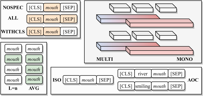
Figure 1: Illustration of the components denoting adopted extraction strategies, including source LM (top right), presence of context (bottom right), special tokens (top left), and layer-wise averaging (bottom left).

Component	Label	Short Description
Source LM	mono	Language-specific (i.e., monolingually pretrained) BERT
	multi	Multilingual BERT, pretrained on 104 languages (with shared subword vocabulary)
Context	iso	Each vocabulary word $w$ is encoded in isolation, without any external context
	aoc-M	Average-over-context: average over word’s encodings from $M$ different contexts/sentences
Subword Tokens	nospec	Special tokens [CLS] and [SEP] are excluded from subword embedding averaging
	all	Both special tokens [CLS] and [SEP] are included into subword embedding averaging
	withcls	[CLS] is included into subword embedding averaging; [SEP] is excluded
Layerwise Avg	avg(L$\leq$n)	Average representations over all Transformer layers up to the $n$-th layer $L_{n}$ (included)
	L$=$n	Only the representation from the layer $L_{n}$ is used

Table 1: Configuration components of word-level embedding extraction, resulting in 24 possible configurations.

In this work, we explore several unsupervised word-level representation extraction strategies and configurations for lexico-semantic tasks (i.e., probes), stemming from different combinations of the components detailed in Table 1 and illustrated in Figure 1. In particular, we assess the impact of: 1) encoding tokens with monolingual LM-pretrained Transformers vs. with their massively multilingual counterparts; 2) providing context around the target word in input; 3) including special tokens like [CLS] and [SEP]; 4) averaging across several layers as opposed to a single layer.

3 Experimental Setup

Pretrained LMs and Languages. Our selection of test languages is guided by the following constraints: a) availability of comparable pretrained (language-specific) monolingual LMs; b) availability of evaluation data; and c) typological diversity of the sample, along the lines of recent initiatives in multilingual NLP (Gerz et al., 2018; Hu et al., 2020; Ponti et al., 2020, inter alia). We work with English (en), German (de), Russian (ru), Finnish (fi), Chinese (zh), and Turkish (tr). We use monolingual uncased BERT Base models for all languages, retrieved from the HuggingFace repository Wolf et al. (2019). All BERT models comprise 12 768-dimensional Transformer layers $\{L_{1}\,\text{(bottom layer)},\dots,L_{12}\,\text{(top)}\}$ plus the input embedding layer ($L_{0}$), and 12 attention heads. We also experiment with multilingual BERT (mBERT) Devlin et al. (2019) as the underlying LM, aiming to measure the performance difference between language-specific and massively multilingual LMs in our lexical probing tasks.

Word Vocabularies and External Corpora. We extract type-level representations in each language for the top 100K most frequent words represented in the respective fastText (FT) vectors, which were trained on lowercased monolingual Wikipedias by Bojanowski et al. (2017). The equivalent vocabulary coverage allows a direct comparison to fastText vectors, which we use as a baseline static WE method in all evaluation tasks. To retain the same vocabulary across all configurations, in aoc variants we back off to the related iso variant for words that have zero occurrences in external corpora.

For all aoc vector variants, we leverage 1M sentences of maximum sequence length 512, which we randomly sample from external corpora: Europarl Koehn (2005) for en, de, fi, available via OPUS Tiedemann (2009); the United Nations Parallel Corpus for ru and zh Ziemski et al. (2016), and monolingual tr WMT17 data Bojar et al. (2017).

Evaluation Tasks. We carry out the evaluation on five standard and diverse lexical semantic tasks:

Task 1: Lexical semantic similarity (LSIM) is the most widespread intrinsic task for evaluation of traditional word embeddings Hill et al. (2015). The evaluation metric is the Spearman’s rank correlation between the average of human-elicited semantic similarity scores for word pairs and the cosine similarity between the respective type-level word vectors. We rely on the recent comprehensive multilingual LSIM benchmark Multi-SimLex Vulić et al. (2020), which covers 1,888 pairs in 13 languages. We focus on en, fi, zh, ru, the languages represented in Multi-SimLex.

Task 2: Word Analogy (WA) is another common intrinsic task. We evaluate our models on the Bigger Analogy Test Set (BATS) Drozd et al. (2016) with 99,200 analogy questions. We resort to the standard vector offset analogy resolution method, searching for the vocabulary word $w_{d}\in V$ such that its vector $d$ is obtained by $argmax_{d}(cos(d,c−a+b))$, where $a$, $b$, and $c$ are word vectors of words $w_{a}$, $w_{b}$, and $w_{c}$ from the analogy $w_{a}:w_{b}=w_{c}:x$. The search space comprises vectors of all words from the vocabulary $V$, excluding $a$, $b$, and $c$. This task is limited to en, and we report Precision@1 scores.

Task 3: Bilingual Lexicon Induction (BLI) is a standard task to evaluate the “semantic quality” of static cross-lingual word embeddings (CLWEs) Gouws et al. (2015); Ruder et al. (2019). We learn “BERT-based” CLWEs using a standard mapping-based approach Mikolov et al. (2013a); Smith et al. (2017) with VecMap Artetxe et al. (2018). BLI evaluation allows us to investigate the “alignability” of monolingual type-level representations extracted for different languages. We adopt the standard BLI evaluation setup from Glavaš et al. (2019): 5K training word pairs are used to learn the mapping, and another 2K pairs as test data. We report standard Mean Reciprocal Rank (MRR) scores for 10 language pairs spanning en, de, ru, fi, tr.

Task 4: Cross-Lingual Information Retrieval (CLIR). We follow the setup of Litschko et al. (2018, 2019) and evaluate mapping-based CLWEs (the same ones as on BLI) in a document-level retrieval task on the CLEF 2003 benchmark. We use a simple CLIR model which showed competitive performance in the comparative studies of Litschko et al. (2019) and Glavaš et al. (2019). It embeds queries and documents as IDF-weighted sums of their corresponding WEs from the CLWE space, and uses cosine similarity as the ranking function. We report Mean Average Precision (MAP) scores for 6 language pairs covering en, de, ru, fi.

Task 5: Lexical Relation Prediction (RELP). We probe if we can recover standard lexical relations (i.e., synonymy, antonymy, hypernymy, meronymy, plus no relation) from input type-level vectors. We rely on a state-of-the-art neural model for RELP operating on type-level embeddings Glavaš and Vulić (2018): the Specialization Tensor Model (STM) predicts lexical relations for pairs of input word vectors based on multi-view projections of those vectors. We use the WordNet-based Fellbaum (1998) evaluation data of Glavaš and Vulić (2018): they contain 10K annotated word pairs balanced by class. Micro-averaged $F_{1}$ scores, averaged across 5 runs for each input vector space (default STM setting), are reported for en and de.

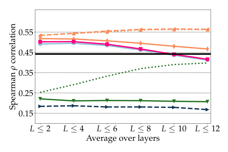
(a) English

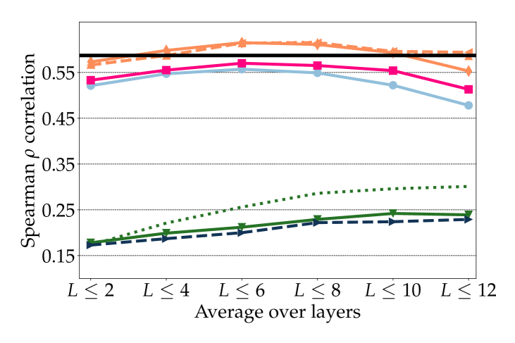
(b) Finnish

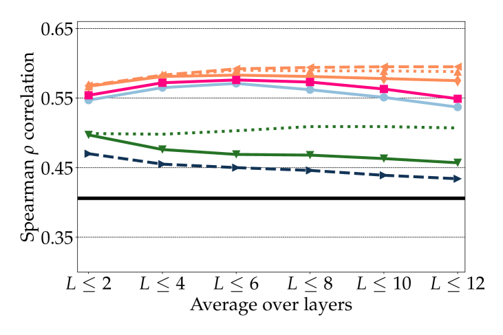
(c) Mandarin Chinese

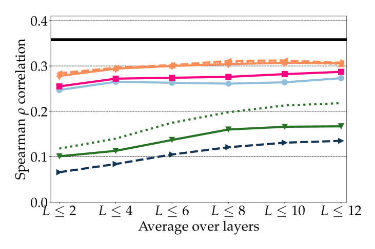
(d) Russian

Figure 2: Spearman’s $\rho$ correlation scores for the lexical semantic similarity task (LSIM) in four languages. For the representation extraction configurations in the legend, see Table 1. Thick solid horizontal lines denote performance of standard monolingual fastText vectors trained on Wikipedia dumps of the respective languages.

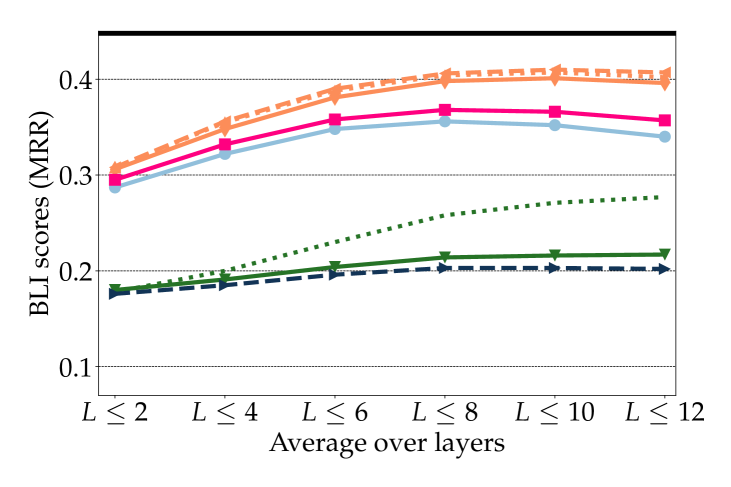
(e) Summary BLI results

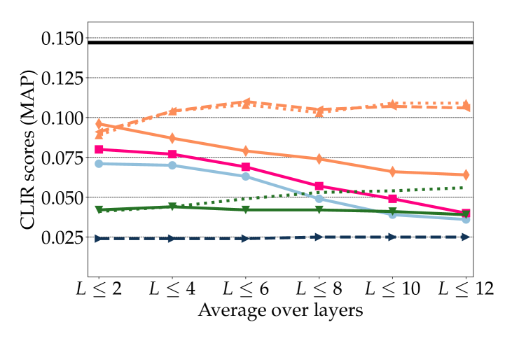
(f) Summary CLIR results

Figure 3: Summary results for the two cross-lingual evaluation tasks: (a) BLI (MRR scores) and (b) CLIR (MAP scores). We report average scores over all language pairs; individual results for each language pair are available in the appendix. Thick solid horizontal lines denote performance of standard fastText vectors in exactly the same cross-lingual mapping setup.

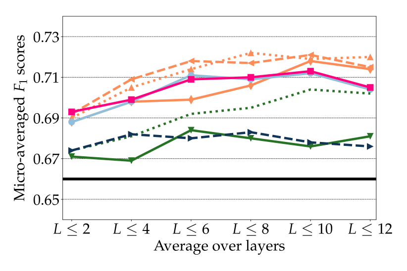
(a) RELP: English

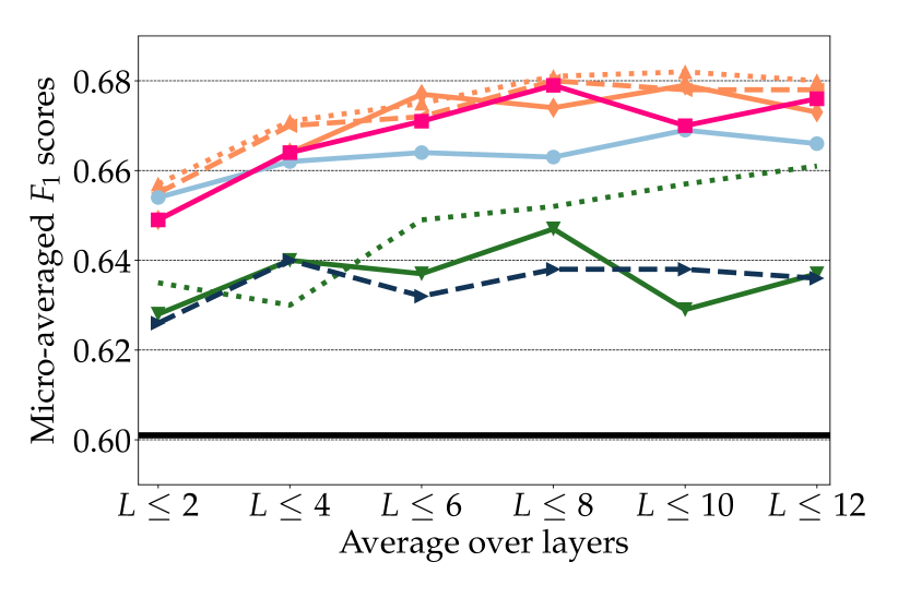
(b) RELP: German

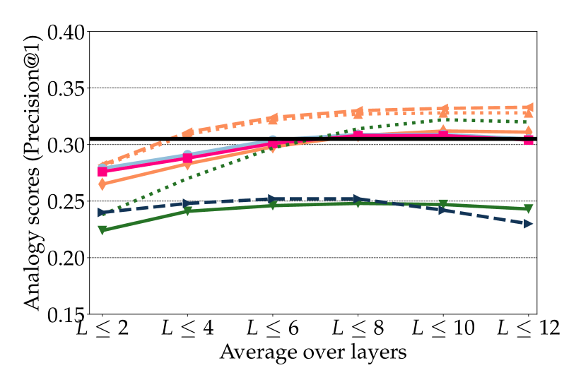
(c) WA: English

Figure 4: Micro-averaged $F_{1}$ scores in the RELP task for (a) en and (b) de. The scores with 768-dim vectors randomly initalized via Xavier init Glorot and Bengio (2010) are 0.473 (en) and 0.512 (de); (c) en WA results.

4 Results and Discussion

A summary of the results is shown in Figure 4 for LSIM, in Figure 2(e) for BLI, in Figure 2(f) for CLIR, in Figure 3(a) and Figure 3(b) for RELP, and in Figure 3(c) for WA. These results offer multiple axes of comparison, and the ensuing discussion focuses on the central questions Q1-Q3 posed in §1.

Monolingual versus Multilingual LMs. Results across all tasks validate the intuition that language-specific monolingual LMs contain much more lexical information for a particular target language than massively multilingual models such as mBERT or XLM-R Artetxe et al. (2020). We see large drops between mono.* and multi.* configurations even for very high-resource languages (en and de), and they are even more prominent for fi and tr.

Encompassing 100+ training languages with limited model capacity, multilingual models suffer from the “curse of multilinguality” Conneau et al. (2020): they must trade off monolingual lexical information coverage (and consequently monolingual performance) for a wider language coverage.

How Important is Context? Another observation that holds across all configurations concerns the usefulness of providing contexts drawn from external corpora, and corroborates findings from prior work Liu et al. (2019b): iso configurations cannot match configurations that average subword embeddings from multiple contexts (aoc-10 and aoc-100). However, it is worth noting that 1) performance gains with aoc-100 over aoc-10, although consistent, are quite marginal across all tasks: this suggests that several word occurrences in vivo are already sufficient to accurately capture its type-level representation. 2) In some tasks, iso configurations are only marginally outscored by their aoc counterparts: e.g., for mono.*.nospec.avg(L$\leq$8) on en–fi BLI or de–tr BLI, the respective scores are 0.486 and 0.315 with iso, and 0.503 and 0.334 with aoc-10. Similar observations hold for fi and zh LSIM, and also in the RELP task.

In RELP, it is notable that ‘BERT-based’ embeddings can recover more lexical relation knowledge than standard FT vectors. These findings reveal that pretrained LMs indeed implicitly capture plenty of lexical type-level knowledge (which needs to be ‘recovered’ from the models); this also suggests why pretrained LMs have been successful in tasks where this knowledge is directly useful, such as NER and POS tagging Tenney et al. (2019); Tsai et al. (2019). Finally, we also note that gains with aoc over iso are much more pronounced for the under-performing multi.* configurations: this indicates that mono models store more lexical information even in absence of context.

How Important are Special Tokens? The results reveal that the inclusion of special tokens [CLS] and [SEP] into type-level embedding extraction deteriorates the final lexical information contained in the embeddings. This finding holds for different languages, underlying LMs, and averaging across various layers. The nospec configurations consistently outperform their all and withcls counterparts, both in iso and aoc-{10, 100} settings.

Our finding at the lexical level aligns well with prior observations on using BERT directly as a sentence encoder Qiao et al. (2019); Singh et al. (2019); Casanueva et al. (2020): while [CLS] is useful for sentence-pair classification tasks, using [CLS] as a sentence representation produces inferior representations than averaging over sentence’s subwords. In this work, we show that [CLS] and [SEP] should also be fully excluded from subword averaging for type-level word representations.

How Important is Layer-wise Averaging? Averaging across layers bottom-to-top (i.e., from $L_{0}$ to $L_{12}$) is beneficial across the board, but we notice that scores typically saturate or even decrease in some tasks and languages when we include higher layers into averaging: see the scores with *.avg(L$\leq$10) and *.avg(L$\leq$12) configurations, e.g., for fi LSIM; en/de RELP, and summary BLI and CLIR scores. This hints to the fact that two strategies typically used in prior work, either to take the vectors only from the embedding layer $L_{0}$ Wu et al. (2020); Wang et al. (2019) or to average across all layers Liu et al. (2019b), extract sub-optimal word representations for a wide range of setups and languages.

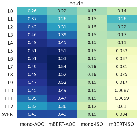
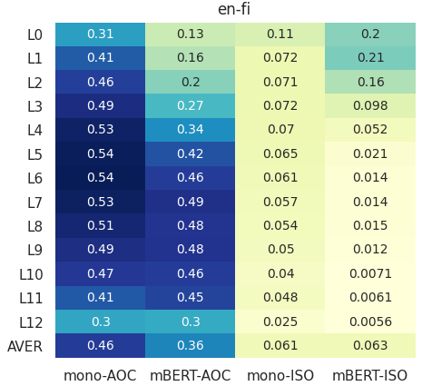
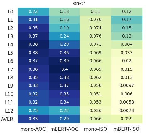
Figure 5: CKA similarity scores of type-level word representations extracted from each layer (using different extraction configurations, see Table 1) for a set of 7K translation pairs in en–de, en–fi, and en–tr from the BLI dictionaries of Glavaš et al. (2019). Additional heatmaps (where random words from two languages are paired) are available in the appendix.

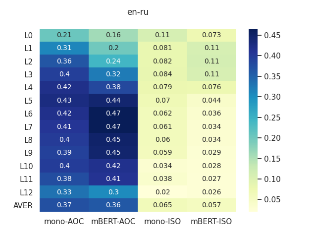
(a) en–ru: Word translation pairs

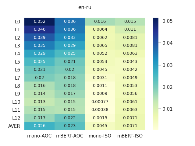
(b) en–ru: Random word pairs

Figure 6: CKA similarity scores of type-level word representations extracted from each layer for a set of (a) 7K en–ru translation pairs from the BLI dictionaries of Glavaš et al. (2019); (b) 7K random en–ru pairs.

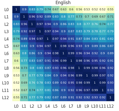
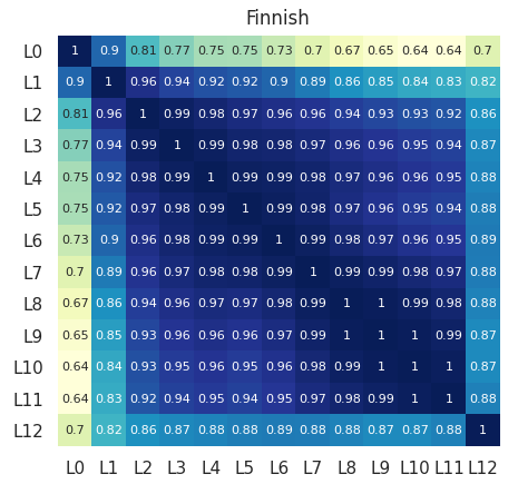
Figure 7: Self-similarity heatmaps: linear CKA similarity of representations for the same word extracted from different Transformer layers, averaged across 7K words for English and Finnish. mono.aoc-100.nospec.

$L_{0}$ $L_{1}$ $L_{2}$ $L_{3}$ $L_{4}$ $L_{5}$ $L_{6}$ $L_{7}$ $L_{8}$ $L_{9}$ $L_{10}$ $L_{11}$ $L_{12}$ LSIM en .503 .513 .505 .510 .505 .484 .459 .435 .402 .361 .362 .372 .390 fi .445 .466 .445 .436 .430 .434 .421 .404 .374 .346 .333 .324 .286 WA en .220 .272 .293 .285 .293 .261 .240 .217 .199 .171 .189 .221 .229 BLI en–de .310 .354 .379 .400 .394 .393 .373 .358 .311 .272 .273 .264 .287 en–fi .309 .339 .360 .367 .369 .345 .329 .303 .279 .252 .231 .194 .192 de–fi .211 .245 .268 .283 .289 .303 .291 .292 .288 .282 .262 .219 .236 CLIR en–de .059 .060 .059 .060 .043 .036 .036 .036 .027 .024 .027 .035 .038 en–fi .038 .040 .022 .018 .011 .008 .006 .006 .005 .002 .003 .002 .007 de–fi .054 .057 .028 .015 .016 .022 .017 .021 .020 .023 .015 .008 .030

Table 2: Task performance of word representations extracted from different Transformer layers for a selection of tasks, languages, and language pairs. Configuration: mono.aoc-100.nospec. Highest scores per row are in bold.

The sweet spot for $n$ in *.avg(L$\leq$n) configurations seems largely task- and language-dependent, as peak scores are obtained with different $n$-s. Whereas averaging across all layers generally hurts performance, the results strongly suggest that averaging across layer subsets (rather than selecting a single layer) is widely useful, especially across bottom-most layers: e.g., $L\leq 6$ with mono.iso.nospec yields an average score of 0.561 in LSIM, 0.076 in CLIR, and 0.432 in BLI; the respective scores when averaging over the 6 top layers are: 0.218, 0.008, and 0.230. This evidence implies that, although scattered across multiple layers, type-level lexical information seems to be concentrated in lower Transformer layers. We investigate these conjectures further in §4.1.

Comparison to Static Word Embeddings. The results also offer a comparison to static FT vectors across languages. The best-performing extraction configurations (e.g., mono.aoc-100.nospec) outperform FT in monolingual evaluations on LSIM (for en, fi, zh), WA, and they also display much stronger performance in the RELP task for both evaluation languages. While the comparison is not strictly apples-to-apples, as FT and LMs were trained on different (Wikipedia) corpora, these findings leave open a provocative question for future work: Given that static type-level word representations can be recovered from large pretrained LMs, does this make standard static WEs obsolete, or are there applications where they are still useful?

The trend is opposite in the two cross-lingual tasks: BLI and CLIR. While there are language pairs for which ‘BERT-based’ WEs outperform FT (i.e., en–fi in BLI, en–ru and fi–ru in CLIR) or are very competitive to FT’s performance (e.g., en–tr, tr–BLI, de–ru CLIR), FT provides higher scores overall in both tasks. The discrepancy between results in monolingual versus cross-lingual tasks warrants further investigation in future work. For instance, is using linear maps, as in standard mapping approaches to CLWE induction, sub-optimal for ‘BERT-based’ word vectors?

Differences across Languages and Tasks. Finally, while we observe a conspicuous amount of universal patterns with configuration components (e.g., mono $>$ multi; aoc $>$ iso; nospec $>$ all, withcls), best-performing configurations do show some variation across different languages and tasks. For instance, while en LSIM performance declines modestly but steadily when averaging over higher-level layers (avg(L$\leq n$), where $n>4$), performance on en WA consistently increases for the same configurations. The BLI and CLIR scores in Figures 2(e) and 2(f) also show slightly different patterns across layers. Overall, this suggests that 1) extracted lexical information must be guided by task requirements, and 2) config components must be carefully tuned to maximise performance for a particular task–language combination.

4.1 Lexical Information in Individual Layers

Evaluation Setup. To better understand which layers contribute the most to the final performance in our lexical tasks, we also probe type-level representations emerging from each individual layer of pretrained LMs. For brevity, we focus on the best performing configurations from previous experiments: {mono, mbert}.{iso, aoc-100}.nospec.

In addition, tackling Q4 from §1, we analyse the similarity of representations extracted from monolingual and multilingual BERT models using the centered kernel alignment (CKA) as proposed by Kornblith et al. (2019). The linear CKA computes similarity that is invariant to isotropic scaling and orthogonal transformation. It is defined as

$$\text{CKA}(X,Y)=\frac{\left\lVert Y^{\top}X\right\rVert^{2}_{\text{F}}}{\left(\left\lVert X^{\top}X\right\rVert_{\text{F}}\left\lVert Y^{\top}Y\right\rVert_{\text{F}}\right)}.$$ (1)

$X,Y\in\mathbb{R}^{s\times d}$ are input matrices spanning $s$ $\ell_{2}$-normalized and mean-centered examples of dimensionality $d=768$. We use CKA in two different experiments: 1) measuring self-similarity where we compute CKA similarity of representations extracted from different layers for the same word; and 2) measuring bilingual layer correspondence where we compute CKA similarity of representations extracted from the same layer for two words constituting a translation pair. To this end, we again use BLI dictionaries of Glavaš et al. (2019) (see §3) covering 7K pairs (training + test pairs).

Discussion. Per-layer CKA similarities are provided in Figure 7 (self-similarity) and Figure 5 (bilingual), and we show results of representations extracted from individual layers for selected evaluation setups and languages in Table 2. We also plot bilingual layer correspondence of true word translations versus randomly paired words for en–ru in Figure 6. Figure 7 reveals very similar patterns for both en and fi, and we also observe that self-similarity scores decrease for more distant layers (cf., similarity of $L_{1}$ and $L_{2}$ versus $L_{1}$ and $L_{12}$). However, despite structural similarities identified by linear CKA, the scores from Table 2 demonstrate that structurally similar layers might encode different amounts of lexical information: e.g., compare performance drops between $L_{5}$ and $L_{8}$ in all evaluation tasks.

The results in Table 2 further suggest that more type-level lexical information is available in lower layers, as all peak scores in the table are achieved with representations extracted from layers $L_{1}-L_{5}$. Much lower scores in type-level semantic tasks for higher layers also empirically validate a recent hypothesis of Ethayarajh (2019) “that contextualised word representations are more context-specific in higher layers.” We also note that none of the results with L=$n$ configurations from Table 1 can match best performing avg(L$\leq$n) configurations with layer-wise averaging. This confirms our hypothesis that type-level lexical knowledge, although predominantly captured by lower layers, is disseminated across multiple layers, and layer-wise averaging is crucial to uncover that knowledge.

Further, Figure 5 and Figure 6 reveal that even LMs trained on monolingual data learn similar representations in corresponding layers for word translations (see the mono.aoc columns). Intuitively, this similarity is much more pronounced with aoc configurations with mBERT. The comparison of scores in Figure 6 also reveals much higher correspondence scores for true translation pairs than for randomly paired words (i.e., the correspondence scores for random pairings are, as expected, random). Moreover, multi CKA similarity scores turn out to be higher for more similar language pairs (cf. en–de versus en–tr multi.aoc columns). This suggests that, similar to static WEs, type-level ‘BERT-based’ WEs of different languages also display topological similarity, often termed approximate isomorphism Søgaard et al. (2018), but its degree depends on language proximity. This also clarifies why representations extracted from two independently trained monolingual LMs can be linearly aligned, as validated by BLI and CLIR evaluation (Table 2 and Figure 4).

We also calculated the Spearman’s correlation between CKA similarity scores for configurations mono.aoc-100.nospec.avg(L$\leq$n), for all $n=0,\ldots,12$, and their corresponding BLI scores on en–fi, en–de, and de–fi. The correlations are very high: $\rho=1.0,0.83,0.99$, respectively. This further confirms the approximate isomorphism hypothesis: it seems that higher structural similarities of representations extracted from monolingual pretrained LMs facilitate their cross-lingual alignment.

5 Further Discussion and Conclusion

What about Larger LMs and Corpora? Aspects of LM pretraining, such as the number of model parameters or the size of pretraining data, also impact lexical knowledge stored in the LM’s parameters. Our preliminary experiments have verified that en BERT-Large yields slight gains over the en BERT-Base architecture used in our work (e.g., peak en LSIM scores rise from 0.518 to 0.531). In a similar vein, we have run additional experiments with two available Italian (it) BERT-Base models with identical parameter setups, where one was trained on 13GB of it text, and the other on 81GB. In en (BERT-Base)–it BLI and CLIR evaluations we measure improvements from 0.548 to 0.572 (BLI), and from 0.148 to 0.160 (CLIR) with the 81GB it model. In-depth analyses of these factors are out of the scope of this work, but they warrant further investigations.

Opening Future Research Avenues. Our study has empirically validated that (monolingually) pretrained LMs store a wealth of type-level lexical knowledge, but effectively uncovering and extracting such knowledge from the LMs’ parameters depends on several crucial components (see §2). In particular, some universal choices of configuration can be recommended: i) choosing monolingual LMs; ii) encoding words with multiple contexts; iii) excluding special tokens; iv) averaging over lower layers. Moreover, we found that type-level WEs extracted from pretrained LMs can surpass static WEs like fastText (Bojanowski et al., 2017).

This study has only scratched the surface of this research avenue. In future work, we plan to investigate how domains of external corpora affect aoc configurations, and how to sample representative contexts from the corpora. We will also extend the study to more languages, more lexical semantic probes, and other larger underlying LMs. The difference in performance across layers also calls for more sophisticated lexical representation extraction methods (e.g., through layer weighting or attention) similar to meta-embedding approaches Yin and Schütze (2016); Bollegala and Bao (2018); Kiela et al. (2018). Given the current large gaps between monolingual and multilingual LMs, we will also focus on lightweight methods to enrich lexical content in multilingual LMs Wang et al. (2020); Pfeiffer et al. (2020).

Appendix A Appendix

URLs to the models and external corpora used in our study are provided in Table 3 and Table 4, respectively. URLs to the evaluation data and task architectures for each evaluation task are provided in Table 5. We also report additional and more detailed sets of results across different tasks, word embedding extraction configurations/variants, and language pairs:

• In Table 6 and Table 7, we provide full BLI results per language pair. All scores are Mean Reciprocal Rank (MRR) scores (in the standard scoring interval, 0.0–1.0).

• In Table 8, we provide full CLIR results per language pair. All scores are Mean Average Precision (MAP) scores (in the standard scoring interval, 0.0–1.0).

• In Table 9, we provide full relation prediction (RELP) results for en and de. All scores are micro-averaged $F_{1}$ scores over 5 runs of the relation predictor Glavaš and Vulić (2018). We also report standard deviation for each configuration.

Finally, in Figures 8-10, we also provide heatmaps denoting bilingual layer correspondence, computed via linear CKA similarity Kornblith et al. (2019), for several en–$L_{t}$ language pairs (see §4.1), which are not provided in the main paper

Language URL en https://huggingface.co/bert-base-uncased de https://huggingface.co/bert-base-german-dbmdz-uncased ru https://huggingface.co/DeepPavlov/rubert-base-cased fi https://huggingface.co/TurkuNLP/bert-base-finnish-uncased-v1 zh https://huggingface.co/bert-base-chinese tr https://huggingface.co/dbmdz/bert-base-turkish-uncased Multilingual https://huggingface.co/bert-base-multilingual-uncased it https://huggingface.co/dbmdz/bert-base-italian-uncased https://huggingface.co/dbmdz/bert-base-italian-xxl-uncased

Table 3: URLs of the models used in our study. The first part of the table refers to the models used in the main experiments throughout the paper, while the second part refers to the models used in side experiments.

Language URL en http://opus.nlpl.eu/download.php?f=Europarl/v8/moses/de-en.txt.zip de http://opus.nlpl.eu/download.php?f=Europarl/v8/moses/de-en.txt.zip ru http://opus.nlpl.eu/download.php?f=UNPC/v1.0/moses/en-ru.txt.zip fi http://opus.nlpl.eu/download.php?f=Europarl/v8/moses/en-fi.txt.zip zh http://opus.nlpl.eu/download.php?f=UNPC/v1.0/moses/en-zh.txt.zip tr http://data.statmt.org/wmt18/translation-task/news.2017.tr.shuffled.deduped.gz it http://opus.nlpl.eu/download.php?f=Europarl/v8/moses/en-it.txt.zip

Table 4: Links to the external corpora used in the study. We randomly sample 1M sentences of maximum sequence length 512 from the corresponding corpora.

Task Evaluation Data and/or Model Link LSIM Multi-SimLex Data: multisimlex.com/ WA BATS Data: vecto.space/projects/BATS/ BLI Data: Dictionaries from Glavaš et al. (2019) Data: github.com/codogogo/xling-eval/tree/master/bli_datasets Model: VecMap Model: github.com/artetxem/vecmap CLIR Data: CLEF 2003 Data: catalog.elra.info/en-us/repository/browse/ELRA-E0008/ Model: Agg-IDF from Litschko et al. (2019) Model: github.com/rlitschk/UnsupCLIR RELP Data: WordNet-based RELP data Data: github.com/codogogo/stm/tree/master/data/wn-ls Model: Specialization Tensor Model Model: github.com/codogogo/stm

Table 5: Links to evaluation data and models.

Configuration en–de en–tr en–fi en–ru de–tr de–fi de–ru fasttext.wiki 0.610 0.433 0.488 0.522 0.358 0.435 0.469 mono.iso.nospec avg(L$\leq$2) 0.390 0.332 0.392 0.409 0.237 0.269 0.291 avg(L$\leq$4) 0.430 0.367 0.438 0.447 0.269 0.311 0.338 avg(L$\leq$6) 0.461 0.386 0.476 0.472 0.299 0.359 0.387 avg(L$\leq$8) 0.472 0.390 0.486 0.487 0.315 0.387 0.407 avg(L$\leq$10) 0.461 0.386 0.483 0.488 0.321 0.395 0.416 avg(L$\leq$12) 0.446 0.379 0.471 0.473 0.323 0.395 0.412 mono.aoc-10.nospec avg(L$\leq$2) 0.399 0.342 0.386 0.403 0.242 0.269 0.292 avg(L$\leq$4) 0.457 0.379 0.448 0.433 0.283 0.322 0.343 avg(L$\leq$6) 0.503 0.399 0.480 0.458 0.315 0.369 0.380 avg(L$\leq$8) 0.527 0.414 0.499 0.461 0.332 0.394 0.391 avg(L$\leq$10) 0.534 0.415 0.498 0.459 0.337 0.401 0.394 avg(L$\leq$12) 0.534 0.416 0.492 0.453 0.337 0.401 0.376 mono.aoc-100.nospec avg(L$\leq$2) 0.401 0.343 0.391 0.398 0.239 0.269 0.293 avg(L$\leq$4) 0.459 0.381 0.449 0.437 0.288 0.325 0.343 avg(L$\leq$6) 0.504 0.403 0.484 0.459 0.318 0.373 0.382 avg(L$\leq$8) 0.532 0.418 0.503 0.462 0.334 0.394 0.389 avg(L$\leq$10) 0.540 0.422 0.504 0.459 0.338 0.402 0.393 avg(L$\leq$12) 0.542 0.426 0.500 0.454 0.343 0.401 0.378 mono.iso.all avg(L$\leq$2) 0.352 0.289 0.351 0.374 0.230 0.265 0.283 avg(L$\leq$4) 0.375 0.317 0.391 0.393 0.264 0.302 0.331 avg(L$\leq$6) 0.386 0.330 0.406 0.407 0.289 0.350 0.376 avg(L$\leq$8) 0.372 0.327 0.409 0.413 0.291 0.370 0.392 avg(L$\leq$10) 0.352 0.320 0.396 0.402 0.290 0.370 0.383 avg(L$\leq$12) 0.313 0.310 0.373 0.394 0.283 0.358 0.371 mono.iso.withcls avg(L$\leq$2) 0.367 0.306 0.368 0.386 0.236 0.272 0.285 avg(L$\leq$4) 0.394 0.339 0.408 0.410 0.267 0.307 0.331 avg(L$\leq$6) 0.406 0.344 0.428 0.425 0.294 0.353 0.381 avg(L$\leq$8) 0.393 0.344 0.430 0.431 0.306 0.369 0.400 avg(L$\leq$10) 0.371 0.336 0.421 0.421 0.303 0.382 0.395 avg(L$\leq$12) 0.331 0.329 0.403 0.409 0.302 0.375 0.387 multi.iso.nospec avg(L$\leq$2) 0.293 0.176 0.176 0.147 0.216 0.203 0.160 avg(L$\leq$4) 0.304 0.184 0.190 0.164 0.219 0.214 0.178 avg(L$\leq$6) 0.315 0.189 0.203 0.198 0.223 0.225 0.198 avg(L$\leq$8) 0.325 0.193 0.209 0.228 0.224 0.235 0.217 avg(L$\leq$10) 0.330 0.194 0.210 0.243 0.220 0.234 0.226 avg(L$\leq$12) 0.333 0.193 0.206 0.248 0.219 0.231 0.227 multi.aoc-10.nospec avg(L$\leq$2) 0.309 0.171 0.172 0.146 0.208 0.200 0.156 avg(L$\leq$4) 0.350 0.186 0.189 0.186 0.224 0.214 0.191 avg(L$\leq$6) 0.389 0.219 0.215 0.240 0.241 0.243 0.225 avg(L$\leq$8) 0.432 0.246 0.251 0.287 0.255 0.263 0.254 avg(L$\leq$10) 0.448 0.258 0.264 0.306 0.260 0.282 0.272 avg(L$\leq$12) 0.456 0.267 0.272 0.316 0.260 0.292 0.284 multi.iso.all avg(L$\leq$2) 0.292 0.173 0.175 0.143 0.209 0.203 0.154 avg(L$\leq$4) 0.301 0.176 0.188 0.155 0.211 0.213 0.171 avg(L$\leq$6) 0.307 0.181 0.198 0.186 0.216 0.221 0.193 avg(L$\leq$8) 0.315 0.184 0.202 0.207 0.213 0.228 0.208 avg(L$\leq$10) 0.318 0.182 0.197 0.216 0.208 0.226 0.215 avg(L$\leq$12) 0.319 0.181 0.189 0.220 0.209 0.220 0.213 mono.iso.nospec (reverse) avg(L$\geq$12) 0.104 – 0.054 – – 0.077 – avg(L$\geq$10) 0.119 – 0.061 – – 0.063 – avg(L$\geq$8) 0.144 – 0.108 – – 0.095 – avg(L$\geq$6) 0.230 – 0.223 – – 0.238 – avg(L$\geq$4) 0.308 – 0.318 – – 0.335 – avg(L$\geq$2) 0.365 – 0.385 – – 0.372 – avg(L$\geq$0) 0.446 – 0.471 – – 0.395 –

Table 6: Results in the BLI task across different language pairs and word vector extraction configurations. MRR scores reported. For clarity of presentation, a subset of results is presented in this table, while the rest (and the averages) are presented in Table 7. avg(L$\leq$n) means that we average representations over all Transformer layers up to the $n$th layer (included), where $L=0$ refers to the embedding layer, $L=1$ to the bottom layer, and $L=12$ to the final (top) layer. Different configurations are described in §2 and Table 1. Additional diagnostic experiments with top-to-bottom layerwise averaging configs (reverse) are run for a subset of languages: {en, de, fi }.

Configuration tr–fi tr–ru fi–ru average fasttext.wiki 0.358 0.364 0.439 0.448 mono.iso.nospec avg(L$\leq$2) 0.237 0.217 0.290 0.306 avg(L$\leq$4) 0.279 0.261 0.337 0.348 avg(L$\leq$6) 0.311 0.288 0.372 0.381 avg(L$\leq$8) 0.334 0.315 0.387 0.398 avg(L$\leq$10) 0.347 0.317 0.392 0.401 avg(L$\leq$12) 0.352 0.319 0.387 0.396 mono.aoc-10.nospec avg(L$\leq$2) 0.247 0.221 0.284 0.308 avg(L$\leq$4) 0.288 0.263 0.331 0.355 avg(L$\leq$6) 0.319 0.294 0.366 0.388 avg(L$\leq$8) 0.334 0.311 0.375 0.404 avg(L$\leq$10) 0.340 0.311 0.379 0.407 avg(L$\leq$12) 0.344 0.310 0.360 0.402 mono.aoc-100.nospec avg(L$\leq$2) 0.244 0.220 0.285 0.308 avg(L$\leq$4) 0.288 0.261 0.333 0.356 avg(L$\leq$6) 0.322 0.291 0.367 0.390 avg(L$\leq$8) 0.338 0.309 0.376 0.406 avg(L$\leq$10) 0.348 0.314 0.377 0.410 avg(L$\leq$12) 0.349 0.311 0.361 0.407 mono.iso.all avg(L$\leq$2) 0.226 0.212 0.284 0.287 avg(L$\leq$4) 0.270 0.254 0.328 0.322 avg(L$\leq$6) 0.302 0.274 0.358 0.348 avg(L$\leq$8) 0.318 0.296 0.371 0.356 avg(L$\leq$10) 0.328 0.303 0.373 0.352 avg(L$\leq$12) 0.328 0.306 0.368 0.340 mono.iso.withcls avg(L$\leq$2) 0.232 0.217 0.285 0.295 avg(L$\leq$4) 0.274 0.257 0.331 0.332 avg(L$\leq$6) 0.307 0.279 0.362 0.358 avg(L$\leq$8) 0.327 0.303 0.377 0.368 avg(L$\leq$10) 0.334 0.314 0.383 0.366 avg(L$\leq$12) 0.340 0.317 0.373 0.357 multi.iso.nospec avg(L$\leq$2) 0.170 0.131 0.127 0.180 avg(L$\leq$4) 0.180 0.135 0.138 0.191 avg(L$\leq$6) 0.188 0.147 0.151 0.204 avg(L$\leq$8) 0.189 0.152 0.164 0.214 avg(L$\leq$10) 0.188 0.153 0.165 0.216 avg(L$\leq$12) 0.188 0.158 0.163 0.217 multi.aoc-10.nospec avg(L$\leq$2) 0.165 0.127 0.130 0.178 avg(L$\leq$4) 0.176 0.146 0.139 0.200 avg(L$\leq$6) 0.192 0.174 0.162 0.230 avg(L$\leq$8) 0.210 0.192 0.185 0.258 avg(L$\leq$10) 0.219 0.198 0.200 0.271 avg(L$\leq$12) 0.223 0.198 0.206 0.277 multi.iso.all avg(L$\leq$2) 0.163 0.126 0.123 0.176 avg(L$\leq$4) 0.175 0.128 0.133 0.185 avg(L$\leq$6) 0.179 0.139 0.142 0.196 avg(L$\leq$8) 0.182 0.144 0.152 0.203 avg(L$\leq$10) 0.178 0.141 0.153 0.203 avg(L$\leq$12) 0.175 0.143 0.150 0.202

Table 7: Results in the bilingual lexicon induction (BLI) task across different language pairs and word vector extraction configurations: Part II. MAP scores reported. For clarity of presentation, a subset of results is presented in this table, while the rest (also used to calculate the averages) is provided in Table 6 in the previous page. avg(L$\leq$n) means that we average representations over all Transformer layers up to the $n$th layer (included), where $L=0$ refers to the embedding layer, $L=1$ to the bottom layer, and $L=12$ to the final (top) layer. Different configurations are described in §2 and Table 1.

Configuration en–de en–fi en–ru de–fi de–ru fi–ru average fasttext.wiki 0.193 0.136 0.118 0.221 0.112 0.105 0.148 mono.iso.nospec avg(L$\leq$2) 0.059 0.075 0.106 0.126 0.086 0.123 0.096 avg(L$\leq$4) 0.061 0.069 0.098 0.111 0.075 0.106 0.087 avg(L$\leq$6) 0.052 0.061 0.079 0.112 0.068 0.102 0.079 avg(L$\leq$8) 0.042 0.048 0.075 0.112 0.063 0.105 0.074 avg(L$\leq$10) 0.036 0.043 0.067 0.107 0.065 0.080 0.066 avg(L$\leq$12) 0.032 0.034 0.059 0.097 0.077 0.083 0.064 mono.aoc-10.nospec avg(L$\leq$2) 0.069 0.078 0.094 0.109 0.078 0.108 0.089 avg(L$\leq$4) 0.076 0.105 0.119 0.112 0.098 0.117 0.104 avg(L$\leq$6) 0.086 0.090 0.129 0.122 0.098 0.125 0.108 avg(L$\leq$8) 0.092 0.073 0.137 0.105 0.100 0.114 0.103 avg(L$\leq$10) 0.095 0.073 0.147 0.102 0.102 0.135 0.109 avg(L$\leq$12) 0.104 0.073 0.139 0.100 0.105 0.131 0.109 mono.aoc-100.nospec avg(L$\leq$2) 0.073 0.081 0.097 0.111 0.078 0.106 0.091 avg(L$\leq$4) 0.078 0.107 0.115 0.107 0.100 0.115 0.104 avg(L$\leq$6) 0.087 0.087 0.127 0.132 0.103 0.123 0.110 avg(L$\leq$8) 0.091 0.076 0.137 0.118 0.101 0.106 0.105 avg(L$\leq$10) 0.099 0.074 0.161 0.103 0.104 0.104 0.107 avg(L$\leq$12) 0.106 0.076 0.146 0.105 0.106 0.100 0.106 mono.iso.all avg(L$\leq$2) 0.044 0.045 0.076 0.095 0.067 0.098 0.071 avg(L$\leq$4) 0.039 0.042 0.079 0.094 0.066 0.100 0.070 avg(L$\leq$6) 0.024 0.034 0.069 0.089 0.066 0.094 0.063 avg(L$\leq$8) 0.018 0.020 0.039 0.068 0.059 0.092 0.049 avg(L$\leq$10) 0.016 0.016 0.030 0.048 0.058 0.067 0.039 avg(L$\leq$12) 0.014 0.013 0.033 0.034 0.064 0.061 0.036 mono.iso.withcls avg(L$\leq$2) 0.050 0.057 0.086 0.106 0.071 0.108 0.080 avg(L$\leq$4) 0.046 0.055 0.084 0.104 0.071 0.102 0.077 avg(L$\leq$6) 0.032 0.042 0.076 0.103 0.066 0.097 0.069 avg(L$\leq$8) 0.025 0.028 0.046 0.086 0.059 0.101 0.057 avg(L$\leq$10) 0.021 0.030 0.037 0.072 0.057 0.079 0.049 avg(L$\leq$12) 0.020 0.016 0.032 0.052 0.045 0.072 0.040 multi.iso.nospec avg(L$\leq$2) 0.110 0.009 0.045 0.057 0.020 0.013 0.042 avg(L$\leq$4) 0.100 0.007 0.075 0.044 0.025 0.011 0.044 avg(L$\leq$6) 0.098 0.007 0.046 0.043 0.029 0.030 0.042 avg(L$\leq$8) 0.088 0.008 0.052 0.043 0.032 0.031 0.042 avg(L$\leq$10) 0.084 0.008 0.051 0.042 0.034 0.026 0.041 avg(L$\leq$12) 0.082 0.006 0.048 0.039 0.037 0.024 0.039 multi.aoc-10.nospec avg(L$\leq$2) 0.127 0.013 0.049 0.027 0.019 0.009 0.041 avg(L$\leq$4) 0.123 0.018 0.055 0.032 0.029 0.008 0.044 avg(L$\leq$6) 0.120 0.018 0.055 0.051 0.042 0.009 0.049 avg(L$\leq$8) 0.123 0.018 0.057 0.053 0.049 0.016 0.053 avg(L$\leq$10) 0.127 0.019 0.062 0.050 0.051 0.018 0.054 avg(L$\leq$12) 0.128 0.021 0.065 0.049 0.052 0.019 0.056 multi.iso.all avg(L$\leq$2) 0.072 0.005 0.032 0.014 0.016 0.004 0.024 avg(L$\leq$4) 0.075 0.004 0.027 0.014 0.022 0.005 0.024 avg(L$\leq$6) 0.065 0.004 0.026 0.015 0.027 0.007 0.024 avg(L$\leq$8) 0.054 0.004 0.035 0.015 0.032 0.008 0.025 avg(L$\leq$10) 0.054 0.005 0.032 0.017 0.035 0.007 0.025 avg(L$\leq$12) 0.058 0.004 0.034 0.018 0.032 0.006 0.025 mono.iso.nospec (reverse) avg(L$\geq$12) 0.005 0.012 – 0.001 – – – avg(L$\geq$10) 0.002 0.002 – 0.001 – – – avg(L$\geq$8) 0.004 0.002 – 0.002 – – – avg(L$\geq$6) 0.014 0.006 – 0.004 – – – avg(L$\geq$4) 0.020 0.012 – 0.016 – – – avg(L$\geq$2) 0.024 0.019 – 0.043 – – – avg(L$\geq$0) 0.032 0.034 – 0.097 – – –

Table 8: Results in the CLIR task across different language pairs and word vector extraction configurations. MAP scores reported; avg(L$\leq$n) means that we average representations over all Transformer layers up to the $n$th layer (included), where $L=0$ refers to the embedding layer, $L=1$ to the bottom layer, and $L=12$ to the final (top) layer. Different configurations are described in §2 and Table 1. Additional diagnostic experiments with top-to-bottom layerwise averaging configs (reverse) are run for a subset of languages: {en, de, fi }.

Configuration en de fasttext.wiki $0.660_{\pm 0.008}$ $0.601_{\pm 0.007}$ random.xavier $0.473_{\pm 0.003}$ $0.512_{\pm 0.008}$ mono.iso.nospec avg(L$\leq$2) $0.688_{\pm 0.007}$ $0.649_{\pm 0.002}$ avg(L$\leq$4) $0.698_{\pm 0.002}$ $0.664_{\pm 0.004}$ avg(L$\leq$6) $0.699_{\pm 0.007}$ $0.677_{\pm 0.006}$ avg(L$\leq$8) $0.706_{\pm 0.003}$ $0.674_{\pm 0.016}$ avg(L$\leq$10) $0.718_{\pm 0.002}$ $0.679_{\pm 0.008}$ avg(L$\leq$12) $0.714_{\pm 0.012}$ $0.673_{\pm 0.003}$ mono.aoc-10.nospec avg(L$\leq$2) $0.690_{\pm 0.007}$ $0.657_{\pm 0.005}$ avg(L$\leq$4) $0.705_{\pm 0.006}$ $0.671_{\pm 0.009}$ avg(L$\leq$6) $0.714_{\pm 0.008}$ $0.675_{\pm 0.014}$ avg(L$\leq$8) $0.722_{\pm 0.004}$ $0.681_{\pm 0.010}$ avg(L$\leq$10) $0.719_{\pm 0.007}$ $0.682_{\pm 0.007}$ avg(L$\leq$12) $0.720_{\pm 0.005}$ $0.680_{\pm 0.007}$ mono.aoc-100.nospec avg(L$\leq$2) $0.692_{\pm 0.007}$ $0.655_{\pm 0.007}$ avg(L$\leq$4) $0.709_{\pm 0.007}$ $0.670_{\pm 0.005}$ avg(L$\leq$6) $0.718_{\pm 0.009}$ $0.672_{\pm 0.008}$ avg(L$\leq$8) $0.717_{\pm 0.003}$ $0.680_{\pm 0.006}$ avg(L$\leq$10) $0.721_{\pm 0.009}$ $0.678_{\pm 0.004}$ avg(L$\leq$12) $0.715_{\pm 0.003}$ $0.678_{\pm 0.006}$ mono.iso.all avg(L$\leq$2) $0.688_{\pm 0.008}$ $0.654_{\pm 0.012}$ avg(L$\leq$4) $0.698_{\pm 0.011}$ $0.662_{\pm 0.008}$ avg(L$\leq$6) $0.711_{\pm 0.005}$ $0.664_{\pm 0.005}$ avg(L$\leq$8) $0.709_{\pm 0.008}$ $0.663_{\pm 0.015}$ avg(L$\leq$10) $0.712_{\pm 0.006}$ $0.669_{\pm 0.003}$ avg(L$\leq$12) $0.704_{\pm 0.005}$ $0.666_{\pm 0.013}$ mono.iso.withcls avg(L$\leq$2) $0.693_{\pm 0.004}$ $0.649_{\pm 0.016}$ avg(L$\leq$4) $0.699_{\pm 0.004}$ $0.664_{\pm 0.006}$ avg(L$\leq$6) $0.709_{\pm 0.002}$ $0.671_{\pm 0.006}$ avg(L$\leq$8) $0.710_{\pm 0.003}$ $0.679_{\pm 0.006}$ avg(L$\leq$10) $0.713_{\pm 0.006}$ $0.670_{\pm 0.007}$ avg(L$\leq$12) $0.705_{\pm 0.005}$ $0.676_{\pm 0.006}$ multi.iso.nospec avg(L$\leq$2) $0.671_{\pm 0.009}$ $0.628_{\pm 0.013}$ avg(L$\leq$4) $0.669_{\pm 0.006}$ $0.640_{\pm 0.004}$ avg(L$\leq$6) $0.684_{\pm 0.010}$ $0.637_{\pm 0.009}$ avg(L$\leq$8) $0.680_{\pm 0.005}$ $0.647_{\pm 0.006}$ avg(L$\leq$10) $0.676_{\pm 0.006}$ $0.629_{\pm 0.008}$ avg(L$\leq$12) $0.681_{\pm 0.005}$ $0.637_{\pm 0.004}$ multi.aoc-10.nospec avg(L$\leq$2) $0.674_{\pm 0.005}$ $0.635_{\pm 0.011}$ avg(L$\leq$4) $0.681_{\pm 0.006}$ $0.630_{\pm 0.007}$ avg(L$\leq$6) $0.692_{\pm 0.008}$ $0.649_{\pm 0.010}$ avg(L$\leq$8) $0.695_{\pm 0.004}$ $0.652_{\pm 0.011}$ avg(L$\leq$10) $0.704_{\pm 0.005}$ $0.657_{\pm 0.012}$ avg(L$\leq$12) $0.702_{\pm 0.005}$ $0.661_{\pm 0.008}$ multi.iso.all avg(L$\leq$2) $0.674_{\pm 0.004}$ $0.626_{\pm 0.014}$ avg(L$\leq$4) $0.682_{\pm 0.009}$ $0.640_{\pm 0.009}$ avg(L$\leq$6) $0.680_{\pm 0.002}$ $0.632_{\pm 0.007}$ avg(L$\leq$8) $0.683_{\pm 0.003}$ $0.638_{\pm 0.010}$ avg(L$\leq$10) $0.678_{\pm 0.007}$ $0.638_{\pm 0.015}$ avg(L$\leq$12) $0.676_{\pm 0.013}$ $0.636_{\pm 0.005}$ mono.iso.nospec (reverse) avg(L$\geq$12) $0.683_{\pm 0.007}$ $0.628_{\pm 0.009}$ avg(L$\geq$10) $0.692_{\pm 0.014}$ $0.628_{\pm 0.008}$ avg(L$\geq$8) $0.688_{\pm 0.016}$ $0.648_{\pm 0.007}$ avg(L$\geq$6) $0.704_{\pm 0.015}$ $0.658_{\pm 0.006}$ avg(L$\geq$4) $0.704_{\pm 0.008}$ $0.668_{\pm 0.007}$ avg(L$\geq$2) $0.707_{\pm 0.008}$ $0.667_{\pm 0.004}$ avg(L$\geq$0) $0.714_{\pm 0.012}$ $0.673_{\pm 0.003}$

Table 9: Results in the relation prediction task (RELP) across different word vector extraction configurations. Micro-averaged $F_{1}$ scores reported , obtained as averages over 5 experimental runs for each configuration; standard deviation is also reported. avg(L$\leq$n) means that we average representations over all Transformer layers up to the $n$th layer (included), where $L=0$ refers to the embedding layer, $L=1$ to the bottom layer, and $L=12$ to the final (top) layer. Different configurations are described in §2 and Table 1. random.xavier are 768-dim vectors for the same vocabularies, randomly initialised via Xavier initialisation Glorot and Bengio (2010).

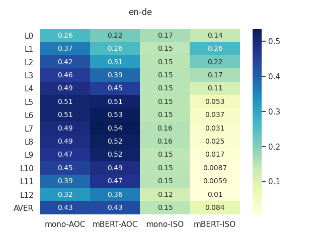
(a) en–de: Word translation pairs

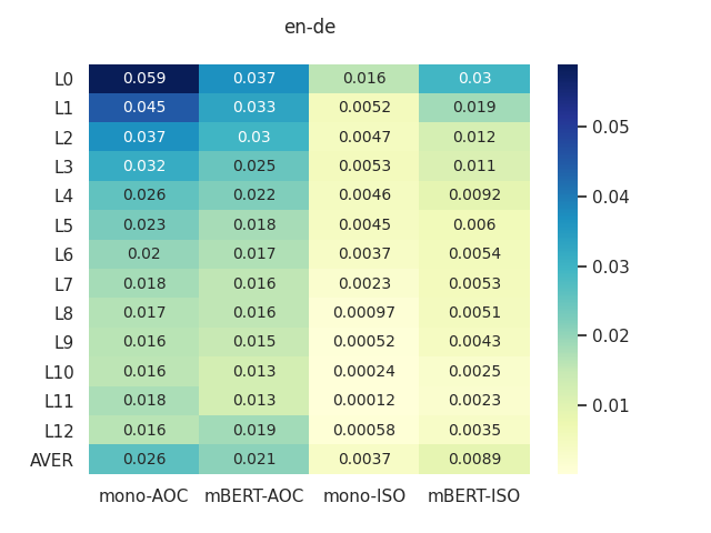
(b) en–de: Random word pairs

Figure 8: CKA similarity scores of type-level word representations extracted from each layer (using different extraction configurations, see Table 1) for a set of (a) 7K en–de translation pairs from the BLI dictionaries of Glavaš et al. (2019); (b) 7K random en–de pairs.

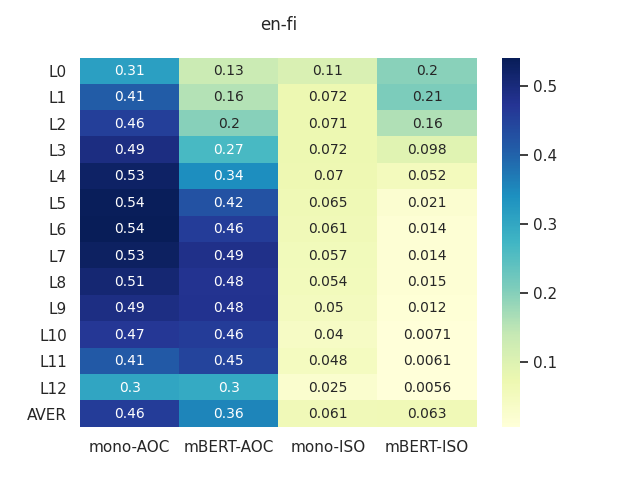
(a) en–fi: Word translation pairs

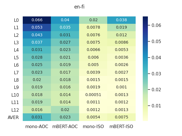
(b) en–fi: Random word pairs

Figure 9: CKA similarity scores of type-level word representations extracted from each layer (using different extraction configurations, see Table 1) for a set of (a) 7K en–fi translation pairs from the BLI dictionaries of Glavaš et al. (2019); (b) 7K random en–fi pairs.

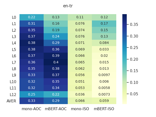
(a) en–tr: Word translation pairs

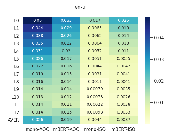
(b) en–tr: Random word pairs

Figure 10: CKA similarity scores of type-level word representations extracted from each layer (using different extraction configurations, see Table 1) for a set of (a) 7K en–tr translation pairs from the BLI dictionaries of Glavaš et al. (2019); (b) 7K random en–tr pairs.

References

- Artetxe et al. (2018) Mikel Artetxe, Gorka Labaka, and Eneko Agirre. 2018. A robust self-learning method for fully unsupervised cross-lingual mappings of word embeddings. In Proceedings of ACL, pages 789–798.
- Artetxe et al. (2020) Mikel Artetxe, Sebastian Ruder, and Dani Yogatama. 2020. On the cross-lingual transferability of monolingual representations. In Proceedings of ACL, pages 4623–4637.
- Belinkov and Glass (2019) Yonatan Belinkov and James R. Glass. 2019. Analysis methods in neural language processing: A survey. Transactions of the Association of Computational Linguistics, 7:49–72.
- Bengio et al. (2003) Yoshua Bengio, Réjean Ducharme, Pascal Vincent, and Christian Jauvin. 2003. A neural probabilistic language model. Journal of Machine Learning Research, 3:1137–1155.
- Bojanowski et al. (2017) Piotr Bojanowski, Edouard Grave, Armand Joulin, and Tomas Mikolov. 2017. Enriching word vectors with subword information. Transactions of the ACL, 5:135–146.
- Bojar et al. (2017) Ondřej Bojar, Rajen Chatterjee, Christian Federmann, Yvette Graham, Barry Haddow, Shujian Huang, Matthias Huck, Philipp Koehn, Qun Liu, Varvara Logacheva, Christof Monz, Matteo Negri, Matt Post, Raphael Rubino, Lucia Specia, and Marco Turchi. 2017. Findings of the 2017 Conference on Machine Translation (WMT17). In Proceedings of WMT, pages 169–214.
- Bollegala and Bao (2018) Danushka Bollegala and Cong Bao. 2018. Learning word meta-embeddings by autoencoding. In Proceedings of COLING, pages 1650–1661.
- Casanueva et al. (2020) Iñigo Casanueva, Tadas Temčinas, Daniela Gerz, Matthew Henderson, and Ivan Vulić. 2020. Efficient intent detection with dual sentence encoders. In Proceedings of the 2nd Workshop on Natural Language Processing for Conversational AI, pages 38–45.
- Chang and Chen (2019) Ting-Yun Chang and Yun-Nung Chen. 2019. What does this word mean? Explaining contextualized embeddings with natural language definition. In Proceedings of EMNLP-IJCNLP, pages 6064–6070.
- Chi et al. (2020) Ethan A. Chi, John Hewitt, and Christopher D. Manning. 2020. Finding universal grammatical relations in multilingual BERT. In Proceedings of ACL, pages 5564–5577.
- Conneau et al. (2020) Alexis Conneau, Kartikay Khandelwal, Naman Goyal, Vishrav Chaudhary, Guillaume Wenzek, Francisco Guzmán, Edouard Grave, Myle Ott, Luke Zettlemoyer, and Veselin Stoyanov. 2020. Unsupervised cross-lingual representation learning at scale. In Proceedings of ACL, pages 8440–8451.
- Devlin et al. (2019) Jacob Devlin, Ming-Wei Chang, Kenton Lee, and Kristina Toutanova. 2019. BERT: Pre-training of deep bidirectional transformers for language understanding. In Proceedings of NAACL-HLT, pages 4171–4186.
- Drozd et al. (2016) Aleksandr Drozd, Anna Gladkova, and Satoshi Matsuoka. 2016. Word embeddings, analogies, and machine learning: Beyond king - man + woman = queen. In Proceedings of COLING, pages 3519–3530.
- Edmiston (2020) Daniel Edmiston. 2020. A systematic analysis of morphological content in BERT models for multiple languages. CoRR, abs/2004.03032.
- Eisenschlos et al. (2019) Julian Eisenschlos, Sebastian Ruder, Piotr Czapla, Marcin Kardas, Sylvain Gugger, and Jeremy Howard. 2019. MultiFiT: Efficient multi-lingual language model fine-tuning. In Proceedings of EMNLP-IJCNLP, pages 5701–5706.
- Ethayarajh (2019) Kawin Ethayarajh. 2019. How contextual are contextualized word representations? Comparing the geometry of BERT, ELMo, and GPT-2 embeddings. In Proceedings of EMNLP-IJCNLP, pages 55–65.
- Fellbaum (1998) Christiane Fellbaum. 1998. WordNet. MIT Press.
- Gerz et al. (2018) Daniela Gerz, Ivan Vulić, Edoardo Maria Ponti, Roi Reichart, and Anna Korhonen. 2018. On the relation between linguistic typology and (limitations of) multilingual language modeling. In Proceedings of EMNLP, pages 316–327.
- Glavaš and Vulić (2018) Goran Glavaš and Ivan Vulić. 2018. Discriminating between lexico-semantic relations with the specialization tensor model. In Proceedings of NAACL-HLT, pages 181–187.
- Glavaš et al. (2019) Goran Glavaš, Robert Litschko, Sebastian Ruder, and Ivan Vulić. 2019. How to (properly) evaluate cross-lingual word embeddings: On strong baselines, comparative analyses, and some misconceptions. In Proceedings of ACL, pages 710–721.
- Glorot and Bengio (2010) Xavier Glorot and Yoshua Bengio. 2010. Understanding the difficulty of training deep feedforward neural networks. In Proceedings of AISTATS, pages 249–256.
- Gouws et al. (2015) Stephan Gouws, Yoshua Bengio, and Greg Corrado. 2015. BilBOWA: Fast bilingual distributed representations without word alignments. In Proceedings of ICML, pages 748–756.
- Hewitt and Manning (2019) John Hewitt and Christopher D. Manning. 2019. A structural probe for finding syntax in word representations. In Proceedings of NAACL-HLT, pages 4129–4138.
- Hill et al. (2015) Felix Hill, Roi Reichart, and Anna Korhonen. 2015. SimLex-999: Evaluating semantic models with (genuine) similarity estimation. Computational Linguistics, 41(4):665–695.
- Hofmann et al. (2020) Valentin Hofmann, Janet B. Pierrehumbert, and Hinrich Schütze. 2020. Generating derivational morphology with BERT. CoRR, abs/2005.00672.
- Hu et al. (2020) Junjie Hu, Sebastian Ruder, Aditya Siddhant, Graham Neubig, Orhan Firat, and Melvin Johnson. 2020. XTREME: A massively multilingual multi-task benchmark for evaluating cross-lingual generalization. In Proceedings of ICML.
- Jawahar et al. (2019) Ganesh Jawahar, Benoît Sagot, and Djamé Seddah. 2019. What does BERT learn about the structure of language? In Proceedings of ACL, pages 3651–3657.
- Kiela et al. (2018) Douwe Kiela, Changhan Wang, and Kyunghyun Cho. 2018. Dynamic meta-embeddings for improved sentence representations. In Proceedings of EMNLP, pages 1466–1477.
- Koehn (2005) Philipp Koehn. 2005. Europarl: A parallel corpus for statistical machine translation. In Proceedings of the 10th Machine Translation Summit (MT SUMMIT), pages 79–86.
- Kornblith et al. (2019) Simon Kornblith, Mohammad Norouzi, Honglak Lee, and Geoffrey E. Hinton. 2019. Similarity of neural network representations revisited. In Proceedings of ICML, pages 3519–3529.
- Kulmizev et al. (2020) Artur Kulmizev, Vinit Ravishankar, Mostafa Abdou, and Joakim Nivre. 2020. Do neural language models show preferences for syntactic formalisms? In Proceedings of ACL, pages 4077–4091.
- Litschko et al. (2018) Robert Litschko, Goran Glavaš, Simone Paolo Ponzetto, and Ivan Vulić. 2018. Unsupervised cross-lingual information retrieval using monolingual data only. In Proceedings of SIGIR, pages 1253–1256.
- Litschko et al. (2019) Robert Litschko, Goran Glavaš, Ivan Vulić, and Laura Dietz. 2019. Evaluating resource-lean cross-lingual embedding models in unsupervised retrieval. In Proceedings of SIGIR, pages 1109–1112.
- Liu et al. (2019a) Nelson F. Liu, Matt Gardner, Yonatan Belinkov, Matthew E. Peters, and Noah A. Smith. 2019a. Linguistic knowledge and transferability of contextual representations. In Proceedings of NAACL-HLT, pages 1073–1094.
- Liu et al. (2019b) Qianchu Liu, Diana McCarthy, Ivan Vulić, and Anna Korhonen. 2019b. Investigating cross-lingual alignment methods for contextualized embeddings with token-level evaluation. In Proceedings of CoNLL, pages 33–43.
- Liu et al. (2019c) Yinhan Liu, Myle Ott, Naman Goyal, Jingfei Du, Mandar Joshi, Danqi Chen, Omer Levy, Mike Lewis, Luke Zettlemoyer, and Veselin Stoyanov. 2019c. RoBERTa: A robustly optimized BERT pretraining approach. CoRR, abs/1907.11692.
- Mickus et al. (2020) Timothee Mickus, Denis Paperno, Mathieu Constant, and Kees van Deemter. 2020. What do you mean, BERT? Assessing BERT as a distributional semantics model. Proceedings of the Society for Computation in Linguistics, 3(34).
- Mikolov et al. (2013a) Tomas Mikolov, Quoc V. Le, and Ilya Sutskever. 2013a. Exploiting similarities among languages for machine translation. arXiv preprint, CoRR, abs/1309.4168.
- Mikolov et al. (2013b) Tomas Mikolov, Ilya Sutskever, Kai Chen, Gregory S. Corrado, and Jeffrey Dean. 2013b. Distributed representations of words and phrases and their compositionality. In Proceedings of NeurIPS, pages 3111–3119.
- Pennington et al. (2014) Jeffrey Pennington, Richard Socher, and Christopher Manning. 2014. Glove: Global vectors for word representation. In Proceedings of EMNLP, pages 1532–1543.
- Peters et al. (2018) Matthew Peters, Mark Neumann, Mohit Iyyer, Matt Gardner, Christopher Clark, Kenton Lee, and Luke Zettlemoyer. 2018. Deep contextualized word representations. In Proceedings of NAACL-HLT, pages 2227–2237.
- Pfeiffer et al. (2020) Jonas Pfeiffer, Ivan Vulić, Iryna Gurevych, and Sebastian Ruder. 2020. MAD-X: An adapter-based framework for multi-task cross-lingual transfer. In Proceedings of EMNLP.
- Pimentel et al. (2020) Tiago Pimentel, Josef Valvoda, Rowan Hall Maudslay, Ran Zmigrod, Adina Williams, and Ryan Cotterell. 2020. Information-theoretic probing for linguistic structure. In Proceedings of ACL, pages 4609–4622.
- Ponti et al. (2020) Edoardo Maria Ponti, Goran Glavaš, Olga Majewska, Qianchu Liu, Ivan Vulić, and Anna Korhonen. 2020. XCOPA: A multilingual dataset for causal commonsense reasoning. In Proceedings of EMNLP.
- Qiao et al. (2019) Yifan Qiao, Chenyan Xiong, Zheng-Hao Liu, and Zhiyuan Liu. 2019. Understanding the behaviors of BERT in ranking. CoRR, abs/1904.07531.
- Qiu et al. (2020) Xipeng Qiu, Tianxiang Sun, Yige Xu, Yunfan Shao, Ning Dai, and Xuanjing Huang. 2020. Pre-trained models for natural language processing: A survey. CoRR, abs/2003.08271.
- Raffel et al. (2019) Colin Raffel, Noam Shazeer, Adam Roberts, Katherine Lee, Sharan Narang, Michael Matena, Yanqi Zhou, Wei Li, and Peter J. Liu. 2019. Exploring the limits of transfer learning with a unified text-to-text transformer. CoRR, abs/1910.10683.
- Reif et al. (2019) Emily Reif, Ann Yuan, Martin Wattenberg, Fernanda B. Viegas, Andy Coenen, Adam Pearce, and Been Kim. 2019. Visualizing and measuring the geometry of BERT. In Proceedings of NeurIPS, pages 8594–8603.
- Rogers et al. (2020) Anna Rogers, Olga Kovaleva, and Anna Rumshisky. 2020. A primer in BERTology: what we know about how BERT works. Transactions of the ACL.
- Ruder et al. (2019) Sebastian Ruder, Ivan Vulić, and Anders Søgaard. 2019. A survey of cross-lingual embedding models. Journal of Artificial Intelligence Research, 65:569–631.
- Singh et al. (2019) Jasdeep Singh, Bryan McCann, Richard Socher, and Caiming Xiong. 2019. BERT is not an interlingua and the bias of tokenization. In Proceedings of the 2nd Workshop on Deep Learning Approaches for Low-Resource NLP (DeepLo 2019), pages 47–55.
- Smith et al. (2017) Samuel L. Smith, David H.P. Turban, Steven Hamblin, and Nils Y. Hammerla. 2017. Offline bilingual word vectors, orthogonal transformations and the inverted softmax. In Proceedings of ICLR (Conference Track).
- Søgaard et al. (2018) Anders Søgaard, Sebastian Ruder, and Ivan Vulić. 2018. On the limitations of unsupervised bilingual dictionary induction. In Proceedings of ACL, pages 778–788.
- Tenney et al. (2019) Ian Tenney, Dipanjan Das, and Ellie Pavlick. 2019. BERT rediscovers the classical NLP pipeline. In Proceedings of ACL, pages 4593–4601.
- Tiedemann (2009) Jörg Tiedemann. 2009. News from OPUS - A collection of multilingual parallel corpora with tools and interfaces. In Proceedings of RANLP, pages 237–248.
- Tsai et al. (2019) Henry Tsai, Jason Riesa, Melvin Johnson, Naveen Arivazhagan, Xin Li, and Amelia Archer. 2019. Small and practical BERT models for sequence labeling. In Proceedings EMNLP-IJCNLP, pages 3632–3636.
- Vaswani et al. (2017) Ashish Vaswani, Noam Shazeer, Niki Parmar, Jakob Uszkoreit, Llion Jones, Aidan N. Gomez, Lukasz Kaiser, and Illia Polosukhin. 2017. Attention is all you need. In Proceedings of NeurIPS, pages 6000–6010.
- Voita and Titov (2020) Elena Voita and Ivan Titov. 2020. Information-theoretic probing with minimum description length. In Proceedings of EMNLP.
- Vulić et al. (2020) Ivan Vulić, Simon Baker, Edoardo Maria Ponti, Ulla Petti, Ira Leviant, Kelly Wing, Olga Majewska, Eden Bar, Matt Malone, Thierry Poibeau, Roi Reichart, and Anna Korhonen. 2020. Multi-Simlex: A large-scale evaluation of multilingual and cross-lingual lexical semantic similarity. Computational Linguistics.
- Wang et al. (2020) Ruize Wang, Duyu Tang, Nan Duan, Zhongyu Wei, Xuanjing Huang, Jianshu Ji, Guihong Cao, Daxin Jiang, and Ming Zhou. 2020. K-Adapter: Infusing knowledge into pre-trained models with adapters. CoRR, abs/2002.01808.
- Wang et al. (2019) Yuxuan Wang, Wanxiang Che, Jiang Guo, Yijia Liu, and Ting Liu. 2019. Cross-lingual BERT transformation for zero-shot dependency parsing. In Proceedings of EMNLP-IJCNLP, pages 5721–5727.
- Wolf et al. (2019) Thomas Wolf, Lysandre Debut, Victor Sanh, Julien Chaumond, Clement Delangue, Anthony Moi, Pierric Cistac, Tim Rault, R’emi Louf, Morgan Funtowicz, and Jamie Brew. 2019. HuggingFace’s Transformers: State-of-the-art natural language processing. ArXiv, abs/1910.03771.
- Wu et al. (2020) Shijie Wu, Alexis Conneau, Haoran Li, Luke Zettlemoyer, and Veselin Stoyanov. 2020. Emerging cross-lingual structure in pretrained language models. In Proceedings of ACL, pages 6022–6034.
- Wu and Dredze (2019) Shijie Wu and Mark Dredze. 2019. Beto, bentz, becas: The surprising cross-lingual effectiveness of BERT. In Proceedings of EMNLP, pages 833–844.
- Yin and Schütze (2016) Wenpeng Yin and Hinrich Schütze. 2016. Learning word meta-embeddings. In Proceedings of ACL, pages 1351–1360.
- Ziemski et al. (2016) Michal Ziemski, Marcin Junczys-Dowmunt, and Bruno Pouliquen. 2016. The United Nations Parallel Corpus v1.0. In Proceedings of LREC.