Towards Theoretically Understanding Why Sgd Generalizes Better Than Adam in Deep Learning

Abstract

It is not clear yet why Adam-alike adaptive gradient algorithms suffer from worse generalization performance than Sgd despite their faster training speed. This work aims to provide understandings on this generalization gap by analyzing their local convergence behaviors. Specifically, we observe the heavy tails of gradient noise in these algorithms. This motivates us to analyze these algorithms through their Lévy-driven stochastic differential equations (SDEs) because of the similar convergence behaviors of an algorithm and its SDE. Then we establish the escaping time of these SDEs from a local basin. The result shows that (1) the escaping time of both Sgd and Adam depends on the Radon measure of the basin positively and the heaviness of gradient noise negatively; (2) for the same basin, Sgd enjoys smaller escaping time than Adam, mainly because (a) the geometry adaptation in Adam via adaptively scaling each gradient coordinate well diminishes the anisotropic structure in gradient noise and results in larger Radon measure of a basin; (b) the exponential gradient average in Adam smooths its gradient and leads to lighter gradient noise tails than Sgd. So Sgd is more locally unstable than Adam at sharp minima defined as the minima whose local basins have small Radon measure, and can better escape from them to flatter ones with larger Radon measure. As flat minima here which often refer to the minima at flat or asymmetric basins/valleys often generalize better than sharp ones [1, 2], our result explains the better generalization performance of Sgd over Adam. Finally, experimental results confirm our heavy-tailed gradient noise assumption and theoretical affirmation.

1 Introduction

Stochastic gradient descent (Sgd) [3, 4] has become one of the most popular algorithms for training deep neural networks [5, 6, 7, 8, 9, 10, 11]. In spite of its simplicity and effectiveness, Sgd uses one learning rate for all gradient coordinates and could suffer from unsatisfactory convergence performance, especially for ill-conditioned problems [12]. To avoid this issue, a variety of adaptive gradient algorithms have been developed that adjust learning rate for each gradient coordinate according to the current geometry curvature of the objective function [13, 14, 15, 16]. These algorithms, especially for Adam, have achieved much faster convergence speed than vanilla Sgd in practice.

Despite their faster convergence behaviors, these adaptive gradient algorithms usually suffer from worse generalization performance than Sgd [17, 12, 18]. Specifically, adaptive gradient algorithms often show faster progress in the training phase but their performance quickly reaches a plateaus on test data. Differently, Sgd usually improves model performance slowly but could achieve higher test performance. One empirical explanation [1, 19, 20, 21] for this generalization gap is that adaptive gradient algorithms tend to converge to sharp minima whose local basin has large curvature and usually generalize poorly, while Sgd prefers to find flat minima and thus generalizes better. However, recent evidence [2, 22] shows that (1) for deep neural networks, the minima at the asymmetric basins/valleys where both steep and flat directions exist also generalize well though they are sharp in terms of their local curvature, and (2) Sgd often converges to these minima. So the argument of the conventional “flat" and “sharp" minima defined on curvature cannot explain these new results. Thus the reason for the generalization gap between adaptive gradient methods and Sgd is still unclear.

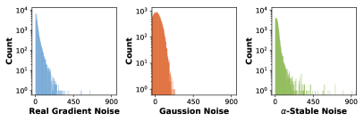
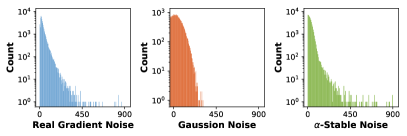
(a) Adam	(b) Sgd

Figure 1: Illustration of gradient noise in Adam and Sgd on AlexNet trained with CIFAR10. (b) is produced under the same setting in [23]. By comparison, one can observe (1) $\alpha$-stable noise can better characterize real gradient noise and (2) Sgd has heavier gradient noise tails than Adam.

In this work, we provide a new viewpoint for understanding the generalization performance gap. We first formulate Adam and Sgd as Lévy-driven stochastic differential equations (SDEs), since the SDE of an algorithm shares similar convergence behaviors of the algorithm and can be analyzed more easily than directly analyzing the algorithm. Then we analyze the escaping behaviors of these SDEs at local minima to investigate the generalization gap between Adam and Sgd, as escaping behaviors determine which basin that an algorithm finally converges to and thus affect the generalization performance of the algorithm. By analysis, we find that compared with Adam, Sgd is more locally unstable and is more likely to converge to the minima at the flat or asymmetric basins/valleys which often have better generalization performance over other type minima. So our results can explain the better generalization performance of Sgd over Adam. Our contributions are highlighted below.

Firstly, this work is the first one that adopts Lévy-driven SDE which better characterizes the algorithm gradient noise in practice, to analyze the adaptive gradient algorithms. Specifically, Fig. 1 shows that the gradient noise in Adam and Sgd, i.e. the difference between the full and stochastic gradients, has heavy tails and can be well characterized by systemic $\alpha$-stable ($\mathcal{S}\alpha\mathcal{S}$) distribution [24]. Based on this observation, we view Adam and Sgd as discretization of the continuous-time processes and formulate the processes as Lévy-driven SDEs to analyze their behaviors. Compared with Gaussian gradient noise assumption in Sgd [25, 26, 27], $\mathcal{S}\alpha\mathcal{S}$ distribution assumption can characterize the heavy-tailed gradient noise in practice more accurately as shown in Fig. 1, and also better explains the different generalization performance of Sgd and Adam as discussed in Sec. 3. This work extends [23, 28] from Sgd on the over-simplified one-dimensional problems to much more complicated adaptive algorithms on high-dimensional problems. It also differs from [29], as [29] considers escaping behaviors of Sgd along several fixed directions, while this work analyzes the dynamic underlying structures in gradient noise that plays an important role in the local escaping behaviors of both Adam and Sgd.

Next, we theoretically prove that for the Lévy-driven SDEs of Adam and Sgd, their escaping time $\Gamma$ from a local basin $\bm{\Omega}$, namely the least time for escaping from the inner of $\bm{\Omega}$ to its outside, is at the order of $\mathcal{O}({\varepsilon^{-\alpha}}\!/m(\bm{\mathcal{W}}))$, where the constant ${\varepsilon}\!\in\!(0,1)$ relies on the learning rate of algorithms and $\alpha$ denotes the tail index of $\mathcal{S}\alpha\mathcal{S}$ distribution. Here $m(\bm{\mathcal{W}})$ is a non-zero Radon measure on the escaping set $\bm{\mathcal{W}}$ of Adam  and Sgd  at the local basin $\bm{\Omega}$ (see Sec. 4.1), and actually negatively relies on the Radon measure of $\bm{\Omega}$. So both Adam and Sgd have small escaping time at the “sharp" minima whose corresponding basins $\bm{\Omega}$ have small Radon measure. It means that Adam and Sgd are actually unstable at “sharp" minima and would escape them to “flatter" ones. Note, the Radon measure of $\bm{\Omega}$ positively depends on the volume of $\bm{\Omega}$. So these results also well explain the observations in [1, 2, 20, 21] that the minima of deep networks found by Sgd often locate at the flat or asymmetric valleys, as their corresponding basins have large volumes and thus large Radon measure.

Finally, our results can answer why Sgd often converges to flatter minima than Adam in terms of Radon measure, and thus explain the generalization gap between Adam and Sgd. Firstly, our analysis shows that even for the same basin $\bm{\Omega}$, Adam often has smaller Radon measure $m(\bm{\mathcal{W}})$ on the escaping set $\bm{\mathcal{W}}$ at $\bm{\Omega}$ than Sgd, as the geometry adaptation in Adam via adaptively scaling each gradient coordinate well diminishes underlying anisotropic structure in gradient noise and leads to smaller $m(\bm{\mathcal{W}})$. Secondly, the empirical results in Sec. 5 and Fig. 1 show that Sgd often has much smaller tail index $\alpha$ of gradient noise than Adam for some optimization iterations and thus enjoys smaller factor ${\varepsilon^{-\alpha}}$. These results together show that Sgd is more locally unstable and would like to converge to flatter minima with larger measure $m(\bm{\mathcal{W}})$ which often refer to the minima at the flat and asymmetric basins/valleys, according with empirical evidences in [12, 30, 31, 17]. Considering the observations in [1, 19, 20, 21] that the minima at the flat and asymmetric basins/valleys often generalize better, our results well explain the generalization gap between Adam and Sgd. Besides, our results also show that Sgd benefits from its anisotropic gradient noise on its escaping behaviors, while Adam does not.

2 Related Work

Adaptive gradient algorithms have become the default optimization tools in deep learning because of their fast convergence speed. But they often suffer from worse generalization performance than Sgd [12, 17, 30, 31]. Subsequently, most works [12, 30, 31, 17, 18] empirically analyze this issue from the argument of flat and sharp minima defined on local curvature in [19] that flat minima often generalize better than sharp ones, as they observed that Sgd often converges to flatter minima than adaptive gradient algorithms, e.g. Adam. However, Sagun et al. [22] and He et al. [2] observed that the minima of modern deep networks at the asymmetric valleys where both steep and flat directions exist also generalize well, and Sgd often converges to these minima. So the conventional flat and sharp argument cannot explain these new results. This work theoretically shows that Sgd tends to converge to the minima whose local basin has larger Radon measure. It well explains the above new observations, as the minima with larger Radon measure often locate at the flat and asymmetric basins/valleys. Moreover, based on our results, exploring invariant Radon measure to parameter scaling in networks could resolve the issue in [32] that flat minima could become sharp via parameter scaling. See more details in Appendix C. Note, Adam could achieve better performance than Sgd when gradient clipping is required [33], e.g. attention models with gradient exploding issue, as adaptation in Adam provides a clipping effect. This work considers a general non-gradient-exploding setting, as it is more practical across many important tasks, e.g. classification.

For theoretical generalization analysis, most works [25, 27, 26, 34] only focus on analyzing Sgd. They formulated Sgd into Brownian motion based SDE via assuming gradient noise to be Gaussian. For instance, Jastrzkebski et al. [26] proved that the larger ratio of learning rate to mini-batch size in Sgd leads to flatter minima and better generalization. But Simsekli et al. [23] empirically found that the gradient noise has heavy tails and can be characterized by $\mathcal{S}\alpha\mathcal{S}$ distribution instead of Gaussian distribution. Chaudhari et al. [27] also claimed that the trajectories of Sgd in deep networks are not Brownian motion. Then Simsekli et al. [23] formulated Sgd as a Lévy-driven SDE and adopted the results in [28] to show that Sgd tends to converge to flat minima on one dimensional problems. Pavlyukevich et al. [29] extended the one-dimensional SDE in [28] and analyzed escaping behaviors of Sgd along several fixed directions, differing from this work that analyzes dynamic underlying structures in gradient noise that greatly affect escaping behaviors of both Adam and Sgd.

The literature targeting theoretically understanding the generalization degeneration of adaptive gradient algorithms are limited mainly due to their more complex algorithms. Wilson et al. [17] constructed a binary classification problem and showed that AdaGrad [13] tend to give undue influence to spurious features that have no effect on out-of-sample generalization. Unlike the above theoretical works that focus on analyzing Sgd only or special problems, we target at revealing the different convergence behaviors of adaptive gradient algorithms and Sgd and also analyzing their different generalization performance, which is of more practical interest especially in deep learning.

3 Lévy-driven SDEs of Algorithms in Deep Learning

In this section, we first briefly introduce Sgd and Adam, and formulate them as discretization of stochastic differential equations (SDEs) which is a popular approach to analyze algorithm behaviors. Suppose the objective function of $n$ components in deep learning models is formulated as

$$\min\nolimits_{\bm{\theta}\in{\mathbb{R}^{d}}}\ \bm{F}(\bm{\theta}):={\frac{1}{n}\sum_{i=1}^{n}f_{i}(\bm{\theta}),}$$ (1)

where $f_{i}(\bm{\theta})$ is the loss of the $i$-th sample. Subsequently, we focus on analyzing Sgd and Adam. Note our analysis technique is applicable to other adaptive algorithms with similar results as Adam.

3.1 Sgd and Adam

As one of the most effective algorithms, Sgd [3] solves problem (1) by sampling a data mini-batch $\mathcal{S}_{t}$ of size $S$ and then running one gradient descent step:

$$\bm{\theta}_{t+1}=\bm{\theta}_{t}-\eta\nabla f_{\mathcal{S}_{t}}(\bm{\theta}_{t}),$$ (2)

where $\nabla f_{\mathcal{S}_{t}}(\bm{\theta}_{t})\!=\!\frac{1}{S}{\sum_{i\in\mathcal{S}_{t}}}\!\nabla f_{i}(\bm{\theta}_{t})$ denotes the gradient on mini-batch $\mathcal{S}_{t}$, and $\eta$ is the learning rate. Recently, to improve the efficiency of Sgd, adaptive gradient algorithms, such as AdaGrad [13], RMSProp [14] and Adam [15], are developed which adjust the learning rate of each gradient coordinate according to the current geometric curvature. Among them, Adam has become the default
training algorithm in deep learning. Specifically, Adam estimates the current gradient $\nabla\bm{F}(\bm{\theta}_{t})$ as

$$\bm{m}_{t}=\beta_{1}\bm{m}_{t-1}+(1-\beta_{1})\nabla f_{\mathcal{S}_{t}}(\bm{\theta}_{t})\ \quad\text{with}\ \bm{m}_{0}=\bm{0}\ \ \text{and}\ \ \beta_{1}\!\in\!(0,1).$$

Then like natural gradient descent [35], Adam adapts itself to the function geometry via a diagonal Fisher matrix approximation $\operatorname{diag}\left(\bm{v}_{t}\right)$ which serves as a preconditioner and is defined as

$$\bm{v}_{t}=\beta_{2}\bm{v}_{t-1}+(1-\beta_{2})[\nabla f_{\mathcal{S}_{t}}(\bm{\theta}_{t})]^{2}\ \quad\text{with}\ \bm{v}_{0}=\bm{0}\ \ \text{and}\ \ \beta_{2}\in(0,1).$$

Next Adam preconditions the problem by scaling each gradient coordinate, and updates the variable

$$\bm{\theta}_{t+1}=\bm{\theta}_{t}-\eta\bm{m}_{t}/(1-\beta_{1}^{t})/\Big{(}{\sqrt{\bm{v}_{t}/(1-\beta_{2}^{t})}}+\epsilon\Big{)}\ \quad\ \text{with a small constant}\ \epsilon.$$ (3)

3.2 Lévy-driven SDEs

Let $\bm{u}_{t}\!=\!\nabla\bm{F}(\bm{\theta}_{t})\!-\!\nabla\!f_{\mathcal{S}_{t}}(\bm{\theta}_{t})$ denote gradient noise. From Sec. 3.1, we can formulate Sgd as follows

$$\bm{\theta}_{t+1}\!=\!\bm{\theta}_{t}-\eta\nabla\bm{F}(\bm{\theta}_{t})+\eta\bm{u}_{t}.$$

To analyze behaviors of an algorithm, one effective approach is to obtain its SDE via making assumptions on $\bm{u}_{t}$ and then analyze its SDE. For instance, to analyze Sgd, most works [25, 27, 26, 34] assume that $\bm{u}_{t}$ obeys a Gaussian distribution $\mathcal{N}(\bm{0},\!\bm{\Sigma}_{t})$ with covariance matrix

$$\bm{\Sigma}_{t}={\frac{1}{S}\Big{[}\frac{1}{n}\sum\nolimits_{i=1}^{n}\nabla f_{i}(\bm{\theta}_{t})\nabla f_{i}(\bm{\theta}_{t})^{T}-\nabla\bm{F}(\bm{\theta}_{t})\nabla\bm{F}(\bm{\theta}_{t})^{T}\Big{]}.}$$

However, both recent work [23] and Fig. 1 show that the gradient noise $\bm{u}_{t}$ has heavy tails and can be better characterized by $\mathcal{S}\alpha\mathcal{S}$ distribution [24]. Moreover, the heavy-tail assumption can also better explain the behaviors of Sgd than Gaussian noise assumption. Concretely, for the SDE of Sgd on the one-dimensional problems, under Gaussian noise assumption its escaping time from a simple quadratic basin respectively exponentially and polynomially depends on the height and width of the basin [36], indicating that Sgd gets stuck at deeper minima as opposed to wider/flatter minima. This contradicts with the observations in [1, 19, 20, 21] that Sgd often converges to flat minima. By contrast, on the same problem, for Lévy-driven SDE, both [23] and this work show that Sgd tends to converge to flat minima instead of deep minima, well explaining the convergence behaviors of Sgd.

Following [23], we also assume $\bm{u}_{t}$ obeys $\mathcal{S}\alpha\mathcal{S}$ distribution but with a time-dependent covariance matrix $\bm{\Sigma}_{t}$ to better characterize the underlying structure in the gradient noise $\bm{u}_{t}$. In this way, when the learning rate $\eta$ is small and $\varepsilon=\eta^{(\alpha-1)/\alpha}$, we can write the Lévy-driven SDE of Sgd as

$$\textsf{d}\bm{\theta}_{t}=-\nabla\bm{F}(\bm{\theta}_{t})+\varepsilon\bm{\Sigma}_{t}\textsf{d}L_{t}.$$ (4)

Here the Lévy motion $L_{t}\in{\mathbb{R}^{d}}$ is a random vector and its $i$-th entry $L_{t,i}$ obeys the $\mathcal{S}\alpha\mathcal{S}(1)$ distribution which is defined through the characteristic function $\mathbb{E}[\exp(i\omega x)]=\exp(-\sigma^{\alpha}|\omega|^{\alpha})$ if $x\sim\mathcal{S}\alpha\mathcal{S}(\sigma)$. Intuitively, the $\mathcal{S}\alpha\mathcal{S}$ distribution is a heavy-tailed distribution with a decay density like $1/|x|^{1+\alpha}$. When the tail index $\alpha$ is 2, $\mathcal{S}\alpha\mathcal{S}(1)$ becomes a Gaussian distribution and thus has stronger data-fitting capacity over Gaussian distribution. In this sense, the SDE of Sgd in [25, 27, 26, 37, 34] is actually a special case of the Lévy-driven SDE in this work. Moreover, Eqn. (4) extends the one-dimensional SDE of Sgd in [23]. Note, Eqn. (4) differs from [29], since it considers dynamic covariance matrix $\bm{\Sigma}_{t}$ in gradient noise and shows great effects of its underlying structure to the escaping behaviors in both Adam and Sgd, while [29] analyzed escaping behaviors of Sgd along several fixed directions.

Similarly, we can derive the SDE of Adam. For brevity, we define $\bm{m}_{t}^{\prime}\!=\!\beta_{1}\bm{m}_{t-1}^{\prime}\!+\!(1-\beta_{1})\nabla\bm{F}(\bm{\theta}_{t})$ with $\bm{m}_{0}^{\prime}=\bm{0}$. Then by the definitions of $\bm{m}_{t}$ and $\bm{m}_{t}^{\prime}$, we can compute

$$\bm{m}_{t}^{\prime}-\bm{m}_{t}={(1-\beta_{1})\sum_{i=0}^{t}\beta_{1}^{t-i}[\nabla\bm{F}(\bm{\theta}_{i})-\nabla f_{\mathcal{S}_{i}}(\bm{\theta}_{i})]}={(1-\beta_{1})\sum_{i=0}^{t}\beta_{1}^{t-i}\bm{u}_{i}}.$$

As noise $\bm{u}_{t}$ has heavy tails, their exponential average should have similar behaviors, which is also illustrated by Fig. 1. So we also assume ${\frac{1}{1-\beta_{{\scriptscriptstyle{1}}}^{t}}}(\bm{m}_{t}^{\prime}-\bm{m}_{t})$ obeys $\mathcal{S}\alpha\mathcal{S}(1)$ distribution with covariance matrix $\bm{\Sigma}_{t}$. Meanwhile, we can write Adam as

$$\bm{\theta}_{t+1}=\bm{\theta}_{t}-{\eta\bm{m}_{t}^{\prime}/\bm{z}_{t}+\eta(\bm{m}_{t}^{\prime}-\bm{m}_{t})/\bm{z}_{t}}\quad\text{with}\quad\bm{z}_{t}\!=\!(1\!-\!\beta_{1}^{t})\Big{(}{\sqrt{\bm{v}_{t}/(1-\beta_{2}^{t})}}+\epsilon\Big{)}.$$

So we can derive the Lévy-driven SDE of Adam:

$$\textsf{d}\bm{\theta}_{t}=-\mu_{t}\bm{Q}_{t}^{-1}\bm{m}_{t}\!+\!\varepsilon\bm{Q}_{t}^{-1}\bm{\Sigma}_{t}\textsf{d}L_{t},\ \ \textsf{d}\bm{m}_{t}=\beta_{1}(\nabla\bm{F}(\bm{\theta}_{t})\!-\!\bm{m}_{t}),\ \ \textsf{d}\bm{v}_{t}=\beta_{2}([\nabla f_{\mathcal{S}_{t}}(\bm{\theta}_{t})]^{2}\!-\!\bm{v}_{t}),$$ (5)

where $\varepsilon\!=\!\eta^{(\alpha-1)/\alpha}$, $\bm{Q}_{t}\!=\!\operatorname{diag}\left(\sqrt{\omega_{t}\bm{v}_{t}}+\epsilon\right)$, $\mu_{t}\!=\!1/(1-e^{-\beta_{1}t})$ and $\omega_{t}=1/(1-e^{-\beta_{2}t})$ are two constants to correct the bias in $\bm{m}_{t}$ and $\bm{v}_{t}$. Note, here we replace $\bm{m}_{t}^{\prime}$ with $\bm{m}_{t}$ for brevity. Appendix B provides more construction details, randomness discussion and shows the fitting capacity of this SDE to Adam. Subsequently, we will analyze escaping behaviors of the SDEs in Eqns. (4) and (5).

4 Analysis for Escaping Local Minima

Now we analyze the local stability of Adam-alike adaptive algorithms and Sgd. Suppose the process $\bm{\theta}_{t}$ in Eqns. (4) and (5) starts at a local basin $\bm{\Omega}$ with a minimum $\bm{\theta}^{*}$, i.e. $\bm{\theta}_{0}\!\in\!\bm{\Omega}$. Here we are particularly interested in the first escaping time $\Gamma$ of $\bm{\theta}_{t}$ produced by an algorithm which reveals the convergence behaviors and generalization performance of the algorithm. Formally, let $\bm{\Omega}^{-\varepsilon^{\gamma}}\!\!=$ $\{\bm{y}\!\in\!\bm{\Omega}\ |\ \textsf{dis}(\partial\bm{\Omega},\bm{y})\!\geq\!{\varepsilon^{\gamma}}\}$ denote the inner part of $\bm{\Omega}$. Then we give two important definitions, i.e. (1) the escaping time $\Gamma$ of the process $\bm{\theta}_{t}$ from the local basin $\bm{\Omega}$ and (2) the escaping set $\bm{\mathcal{W}}$ at $\bm{\Omega}$, as

$$\Gamma=\inf\{t\geq 0\ |\ \bm{\theta}_{t}\notin\bm{\Omega}^{-\varepsilon^{\gamma}}\}\quad\text{and}\quad\bm{\mathcal{W}}=\{\bm{y}\in{\mathbb{R}^{d}}\ |\ \bm{Q}_{\bm{\theta}^{*}}^{-1}\bm{\Sigma}_{\bm{\theta}^{*}}\bm{y}\notin\bm{\Omega}^{-\varepsilon^{\gamma}}\},$$ (6)

where the constant $\gamma>0$ satisfies $\lim_{{\varepsilon}\rightarrow 0}{\varepsilon^{\gamma}}=0$, $\bm{\Sigma}_{\bm{\theta}^{*}}$ $=\!\lim_{\bm{\theta}_{t}\rightarrow\bm{\theta}^{*}}\!\bm{\Sigma}_{t}$ for both Sgd and Adam, and $\bm{Q}_{\bm{\theta}^{*}}\!\!=\bm{I}$ for Sgd and $\bm{Q}_{\bm{\theta}^{*}}\!\!=\!\lim_{\bm{\theta}_{t}\rightarrow\bm{\theta}^{*}}\!\bm{Q}_{t}$ for Adam. Then we define Radon measure [38].

Definition 1.

If a measure $m(\mathcal{V})$ defined on Hausdorff topological space $\bm{\mathcal{X}}$ obeys (1) inner regular, i.e. $m(\mathcal{V})\!=\!\sup_{\mathcal{U}\subseteq\mathcal{V}}\!m(\mathcal{U})$, (2) outer regular, i.e. $m(\mathcal{V})\!=\!\inf_{\mathcal{V}\subseteq\mathcal{U}}\!m(\mathcal{U})$, and (3) local finiteness, i.e. every point of $\bm{\mathcal{X}}$ has a neighborhood $\mathcal{U}$ with finite $m(\mathcal{U})$, then $m(\mathcal{V})$ is a Radon measure.

Then we define non-zero Radon measure which further obeys $m(\mathcal{U})\!<\!m(\mathcal{V})$ if $\mathcal{U}\!\subset\!\mathcal{V}$. Since larger set has larger volume, $m(\mathcal{U})$ positively depends on the volume of the set $\mathcal{U}$. Let $m(\bm{\mathcal{W}})$ be a non-zero Radon measure on the set $\bm{\mathcal{W}}$. Then we first introduce two mild assumptions for analysis.

Assumption 1.

For both Adam and Sgd, suppose the objective $\bm{F}(\bm{\theta})$ is a upper-bounded non-negative loss, and is locally $\mu$-strongly convex and $\ell$-smooth in the basin $\bm{\Omega}$.

Assumption 2.

For Adam, suppose its process $\bm{\theta}_{t}$ satisfies ${\int_{0}^{\Gamma}\big{\langle}\frac{\nabla\bm{F}(\bm{\theta}_{s})}{1+\bm{F}(\bm{\theta}_{s})},}\mu_{s}{\bm{Q}_{s}^{-1}}\bm{m}_{s}\big{\rangle}\textsf{d}s\geq 0$ almost sure, and its parameters $\beta_{1}$ and $\beta_{2}$ obey $\beta_{1}\leq\beta_{2}\leq 2\beta_{1}$. Moreover, for Adam, we assume $\|\bm{m}_{t}-\widehat{\bm{m}}_{t}\|\leq\tau_{m}\|{\int_{0}^{t-}}(\bm{m}_{s}-\widehat{\bm{m}}_{s})\textsf{d}s\|$ and $\|\widehat{\bm{m}}_{t}\|\geq\tau\|\nabla\bm{F}(\widehat{\bm{\theta}}_{t})\|$ where $\widehat{\bm{m}}_{t}$ and $\widehat{\bm{\theta}}_{t}$ are obtained by Eqn. (5) with ${\varepsilon}=0$. Each coordinate $\bm{v}_{t,i}$ of $\bm{v}_{t}$ in Adam obeys $v_{\min}\leq\sqrt{\bm{v}_{t,i}}\leq v_{\max}$ $(\forall i,t)$.

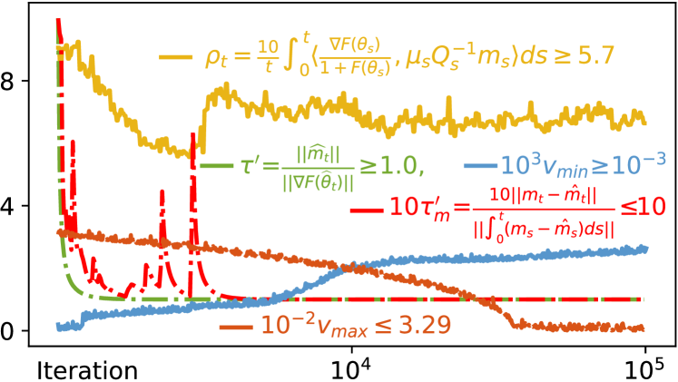
Figure 2: Empirical investigation of Assumption 2 on Adam.

Assumption 1 is very standard for analyzing stochastic optimization [39, 40, 41, 42, 43, 44] and network analysis [45, 46, 47, 48]. In Assumption 2, we indeed require similar directions of gradient estimate $\bm{m}_{t}$ and full gradient $\nabla\bm{F}(\bm{\theta}_{t})$ in Adam in most cases, as we assume their inner product is non-negative along the iteration trajectory. So this assumption can be satisfied in practice. To analyze the processes $\bm{\theta}_{t}$ and $\widehat{\bm{\theta}}_{t}$ in Adam, we make an assumption on the distance between their corresponding gradient estimates $\bm{m}_{t}$ and $\widehat{\bm{m}}_{t}$ which can be easily fulfilled by their definitions. Then for Adam, we mildly assume its estimated $\bm{v}_{t}$ to be bounded. For $v_{\min}$, we indeed allow $v_{\min}=0$ because of the small constant $\epsilon$. The relation $\beta_{1}\leq\beta_{2}\leq 2\beta_{1}$ is also satisfied under the default setting of Adam. Actually, we also empirically investigate Assumption 2 on Adam. In Fig. 2, we report the values of $\rho_{t}=\frac{10}{t}\int_{0}^{\Gamma}\!\!\big{\langle}\frac{\nabla\bm{F}(\bm{\theta}_{s})}{1+\bm{F}(\bm{\theta}_{s})},\mu_{s}{\bm{Q}_{s}^{-1}}\bm{m}_{s}\big{\rangle}ds$, $\tau_{m}^{\prime}=\frac{\|\bm{m}_{t}-\widehat{\bm{m}}_{t}\|}{\|{\int_{0}^{t-}}\!\!(\bm{m}_{s}-\widehat{\bm{m}}_{s})\textsf{d}s\|}$, $\tau^{\prime}=\frac{\|\widehat{\bm{m}}_{t}\|}{\|\!\nabla\!\bm{F}(\widehat{\bm{\theta}}_{t})\|}$, $v_{\min}=\min_{i}\sqrt{\bm{v}_{t,i}},v_{\max}=\max_{i}\sqrt{\bm{v}_{t,i}}$ in the SDE of Adam on the 4-layered fully connected networks with width 20. Note that we scale some values of $\rho_{t}$, $\tau_{m}^{\prime}$, $\tau^{\prime}$, $v_{\min}$ and $v_{\max}$ so that we can plot them in one figures. From Fig. 2, one can observe that $\rho_{t},\tau^{\prime}$ and $v_{\min}$ are well lower bounded, and $\tau_{m}^{\prime}$ and $v_{\max}$ are well upper bounded. These results demonstrate the validity of Assumption 2.

With these two assumptions, we analyze the escaping time $\Gamma$ of process $\bm{\theta}_{t}$ and summarize the main results in Theorem 1. For brevity, we define a group of key constants for Sgd and Adam: $\kappa_{1}\!=\!\ell$ and $\kappa_{2}\!=\!2\mu$ in Sgd, $\kappa_{1}\!=\!\frac{c_{1}\ell}{(v_{\min}+\epsilon)|\tau_{m}-1|}$ and $\kappa_{2}\!=\!\frac{2\mu\tau}{\beta_{1}\left(v_{\max}+\epsilon\right)+\mu\tau}(\beta_{1}\!-\!\frac{\beta_{2}}{4})$ in Adam with a constant $c_{1}$.

Theorem 1.

Suppose Assumptions 1 and 2 hold. Let $\Theta({\varepsilon^{-1}})\!=\!\frac{2}{\alpha}{\varepsilon^{\alpha}}$, $\rho_{0}\!=\!\frac{1}{16(1+c_{2}\kappa_{1})}$ and $\ln\!\big{(}\frac{2\Delta}{\mu{\varepsilon^{1\!/3}}}\big{)}\!\leq\!\kappa_{2}{\varepsilon^{-\frac{1}{3}}}$ with $\Delta\!=\!\bm{F}(\bm{\theta}_{0})$ $-\bm{F}(\bm{\theta}^{*})$ and a constant $c_{2}$. Then for any $\bm{\theta}_{0}\!\in\bm{\Omega}^{-2\varepsilon^{\gamma}}$, $u>\!-1$, ${\varepsilon}\in(0,{\varepsilon}_{0}]$, $\gamma\in(0,\gamma_{0}]$ and $\rho\in(0,\rho_{0}]$ satisfying ${\varepsilon^{\gamma}}\leq\rho_{0}$ and $\lim_{{\varepsilon}\rightarrow 0}\rho=0$, Sgd in (4) and Adam in (5) obey

$${\frac{1-\rho}{1+u+\rho}}\leq\mathbb{E}\left[\exp{\left(-um(\bm{\mathcal{W}})\Theta({\varepsilon^{-1}})\Gamma\right)}\right]\leq{\frac{1+\rho}{1+u-\rho}}.$$

See its proof in Appendix E.1. By setting ${\varepsilon}$ small, Theorem 1 shows that for both Adam and Sgd, the upper and lower bounds of their expected escaping time $\Gamma$ are at the order of $\mathcal{O}\big{(}\frac{1}{m(\bm{\mathcal{W}})\Theta({\varepsilon^{-1}})}\big{)}$. Note, $m(\bm{\mathcal{W}})$ has different values for Sgd and Adam due to their different $\bm{Q}_{\bm{\theta}^{*}}$ in Eqn. (6). If the escaping time $\Gamma$ is very large, it means that the algorithm cannot well escape from the basin $\bm{\Omega}$ and would get stuck in $\bm{\Omega}$. Moreover, given the same basin $\bm{\Omega}$, if one algorithm has smaller escaping time $\Gamma$ than other algorithms, then it is more locally unstable and would faster escape from this basin to others. In the following sections, we discuss the effects of the geometry adaptation and the gradient noise structure of Adam and Sgd to the escaping time $\Gamma$ which are respectively reflected by the factors $m(\bm{\mathcal{W}})$ and $\Theta({\varepsilon^{-1}})$. Our results show that Sgd has smaller escaping time than Adam and can better escape from local basins with small Radon measure to those with lager Radon measure.

4.1 Preference to Flat Minima

To interpret Theorem 1, we first define the “flat" minima in this work in terms of Radon measure.

Definition 2.

​A minimum $\bm{\theta}^{*}\!\in\!\bm{\Omega}$ is said to be flat if its basin $\bm{\Omega}$ has large nonzero Radon measure.

Due to the factor $m(\bm{\mathcal{W}})$ in Theorem 1, both Adam and Sgd have large escaping time $\Gamma$ at the “flat" minima. Specifically, if the basin $\bm{\Omega}$ has larger Radon measure, then the complementary set $\bm{\mathcal{W}}^{c}=$ $\{\bm{y}\!\in\!{\mathbb{R}^{d}}\ |\ \bm{Q}_{\bm{\theta}^{*}}^{-1}\bm{\Sigma}_{\bm{\theta}^{*}}\bm{y}\!\in\!\bm{\Omega}^{-\varepsilon^{\gamma}}\}$ of $\bm{\mathcal{W}}$ also has larger Radon measure. Meanwhile, the Radon measure on $\bm{\mathcal{W}}^{c}\!\cup\!\bm{\mathcal{W}}$ is a constant, meaning the larger $m(\bm{\mathcal{W}}^{c})$ the smaller $m(\bm{\mathcal{W}})$. So Adam and Sgd have larger escaping time at “flat" minima. Thus, they would escape “sharp" minima due to their smaller escaping time, and tend to converge to “flat" ones. Since for basin $\bm{\Omega}$, its Radon measure positively relies on its volume, $m(\bm{\mathcal{W}})$ negatively depends on the volume of $\bm{\Omega}$. So Adam and Sgd are more stable at the minima with larger basin $\bm{\Omega}$ in terms of volume. This can be intuitively understood: for the process $\bm{\theta}_{t}$, the volume of the basin determines the necessary jump size of the Lévy motion $L_{t}$ in the SDEs to escape, which means the larger the basin the harder for an algorithm to escape.

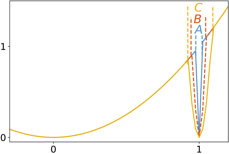
Figure 3: $f(x)\!=\!\min(x^{2},a(x-1)^{2})$

To investigate the above conclusion, namely, positive dependence of the escaping time $\Gamma$ to the Radon measure of a basin, we construct a function $f(x)=\min(x^{2},a(x-1)^{2})$ which has two local basins at the points $x=0$ and $x=1$ as illustrated in Fig. 3. By setting $a=10^{5},500,150$, we obtain three basins $A$, $B$ and $C$, where their Radon measures obey $m(A)<m(B)<m(C)$ because their volumes satisfies $\textsc{V}(A)<\textsc{V}(B)<\textsc{V}(C)$. Then we run SDE of SGD with initialization $x_{0}=1$ for 2000 iterations, and repeat 1000 times. For the three basins $A$, $B$ and $C$ with same Lévy noise, the escaping probabilities of SDE for jumping outside are $100\%$, $65.6\%$ and $10.1\%$, and the average iterations for successful escaping on $A$, $B$ and $C$ are $122$, $457$ and $1898$. For SDE of Adam and Sgd-M(SGD with momentum), we obtain similar observations and do not report them for avoid needless duplication. These results confirm our theory: the larger Radon measure of the basin, the harder to escape.

Note the “flat" minima here is defined on Radon measure, and differ from the conventional flat ones whose local basins have no large curvature (no large eigenvalues in its Hessian matrix). In most cases, the flat minima here consist of the conventional flat ones and the minma at the asymmetric basins/valleys since local basins of these minima often have large volumes and thus larger Radon measures. Accordingly, our theoretical results can well explain the phenomenons observed in many works [12, 30, 31, 17, 22, 2] that Sgd often converges to the minima at the flat or asymmetric valleys which is interpreted by our theory to have larger Radon measure and attract Sgd to stay at these places. In contrast, the conventional flat argument cannot explain asymmetric valleys, as asymmetric valleys means sharp minima under the conventional definition and should be avoided by Sgd.

4.2 Analysis of Generalization Gap between Adam and Sgd

Theorem 1 can also well explain the generalization gap between Adam-alike adaptive algorithms and Sgd. That is, compared with Sgd, the minima given by Adam often suffer from worse test performance [12, 30, 31, 17, 18]. On one hand, the observations in [1, 19, 20, 21] show that the minima at the flat or asymmetric basins/valleys often enjoy better generalization performance than others. On the other hand, Theorem 1 shows that Adam and Sgd can escape sharp minima to flat ones with larger Radon measure. As aforementioned, flat minima in terms of Radon measure often refer to the minima at the flat or asymmetric basins/valleys. This implies that if one algorithm can escape the current minima faster, it is more likely for the algorithm to find flatter minima. These results together show the benefit of faster escaping behaviors of an algorithm to its generalization performance.

According to Theorem 1, two main factors, i.e. the gradient noise and geometry adaptation respectively reflected by the factors $\Theta({\varepsilon^{-1}})\!=\!\frac{2}{\alpha}{\varepsilon^{-\alpha}}$ and $m(\bm{\mathcal{W}})$, affects the escaping time $\Gamma$ of both Adam and Sgd. We first look at the factor $\Theta({\varepsilon^{-1}})$ in the escaping time $\Gamma$. As illustrated in Fig. 4 in Sec. 5, the gradient noise in Sgd enjoys very similar tail index $\alpha$ with Adam for most optimization iterations, but it has much smaller tail index $\alpha$ than Adam  for some iterations, which means Sgd has larger Lévy discontinuous jumps in these iterations and thus enjoys smaller escaping time $\Gamma$. This different tail property of gradient noise in these algorithms are caused by the following reason. Sgd assumes the gradient noise $\bm{u}_{t}\!=\!\nabla\bm{F}(\bm{\theta}_{t})\!-\!\nabla f_{\mathcal{S}_{t}}(\bm{\theta}_{t})$ at one iteration has heavy tails, while Adam considers the exponential gradient noise $\frac{1-\beta_{1}}{1-\beta_{1}^{t}}\sum_{i=0}^{t}\!\beta_{1}^{t-i}\bm{u}_{i}$ which indeed smooths gradient noise over the iteration trajectory and prevents large occasional gradient noise. In this way, Sgd reveals heavier tails of gradient noise than Adam and thus has smaller tail index $\alpha$ for some optimization iterations, helping escaping behaviors. Moreover, to guarantee convergence, Adam needs to use smaller learning rate $\eta$ than Sgd due to the geometry adaptation in Adam, e.g. default learning rate $10^{-3}$ in Adam and $10^{-2}$ in Sgd, leading to smaller $\varepsilon\!=\!\eta^{(\alpha-1)/\alpha}$ and thus larger escaping time $\Gamma$ in Adam. Thus, compared with Adam, Sgd is more locally unstable and will converge to flatter minima which often locate at the flat or asymmetric basins/valleys and enjoy better generalization performance [1, 19, 20, 21].

Besides, the factor $m(\bm{\mathcal{W}})$ also plays an important role in the generalization degeneration phenomenon of Adam. W.o.l.g., assume the minimizer $\bm{\theta}^{*}=\bm{0}$ in the basin $\bm{\Omega}$. As the local basin $\bm{\Omega}$ is often small, following [49, 34] we adopt second-order Taylor expansion to approximate $\bm{\Omega}$ as a quadratic basin with center $\bm{\theta}^{*}$, i.e.  $\bm{\Omega}\!=\!\big{\{}\bm{y}\ |\ \bm{F}(\bm{\theta}^{*})\!+\!\frac{1}{2}\bm{y}^{T}\bm{H}(\bm{\theta}^{*})\bm{y}\!\leq\!h(\bm{\theta}^{*})\big{\}}$ with a basin height $h(\bm{\theta}^{*})$ and Hessian matrix $\bm{H}(\bm{\theta}^{*})$ at $\bm{\theta}^{*}$. Then for Sgd, since $\bm{Q}_{\bm{\theta}^{*}}=\bm{I}$ in Eqn. (6), its corresponding escaping set $\bm{\mathcal{W}}$ is

$$\bm{\mathcal{W}}_{\textsc{Sgd}}=\big{\{}\bm{y}\in{\mathbb{R}^{d}}\ |\ \bm{y}^{T}\bm{\Sigma}_{\bm{\theta}^{*}}\bm{H}(\bm{\theta}^{*})\bm{\Sigma}_{\bm{\theta}^{*}}\bm{y}\geq h_{f}^{*}\big{\}}$$ (7)

with $h_{f}^{*}\!=\!2(h(\bm{\theta}^{*}\!)\!-\!\bm{F}(\bm{\theta}^{*}\!))$, while according to Eqn. (6), Adam has escaping set

$$\bm{\mathcal{W}}_{\!\textsc{Adam}}=\{\bm{y}\in{\mathbb{R}^{d}}\ \!|\ \!\bm{y}^{T}\bm{\Sigma}_{\bm{\theta}^{*}}\bm{Q}_{\bm{\theta}^{*}}^{-1}\bm{H}(\bm{\theta}^{*})\bm{Q}_{\bm{\theta}^{*}}^{-1}\bm{\Sigma}_{\bm{\theta}^{*}}\bm{y}\geq h_{f}^{*}\}.$$ (8)

Then we prove that for most time interval except the jump time, the current variable $\bm{\theta}_{t}$ is indeed close to the minimum $\bm{\theta}^{*}$. Specifically, we first decompose the Lévy process $L_{t}$ into two components $\bm{\xi}_{t}$ and $\bm{\zeta}_{t}$, i.e. $L_{t}=\bm{\xi}_{t}+\bm{\zeta}_{t}$, with the jump sizes $\|\bm{\xi}_{t}\|\!<\!{\varepsilon^{-\delta}}$ and $\|\bm{\zeta}_{t}\|\!\geq\!{\varepsilon^{-\delta}}$ ($\delta\!\in\!(0,1)$). In this way, the stochastic process $\bm{\xi}$ does not departure from $\bm{\theta}_{t}$ a lot due to its limited jump size. The process $\bm{\zeta}$ is a compound Poisson process with intensity $\Theta({\varepsilon}^{-\delta})\!=\!\int_{\|\bm{y}\|\geq{\varepsilon^{-\delta}}}\!\nu(\textsf{d}\bm{y})\!=\!{\int}_{\|\bm{y}\|\geq{\varepsilon^{-\delta}}}\frac{\textsf{d}\bm{y}}{\|\bm{y}\|^{1+\alpha}}\!=\!\frac{2}{\alpha}{\varepsilon^{\alpha\delta}}$ and jumps distributed according to the law of $1/\Theta({\varepsilon}^{-\delta})$. Specifically, let $0\!=\!t_{0}\!<\!t_{1}\!<\!\cdots\!<\!t_{k}\!<\!\cdots$ denote the time of successive jumps of $\bm{\zeta}$. Then the inner-jump time intervals $\sigma_{k}\!=$ $t_{k}-t_{k-1}$ are i.i.d. exponentially distributed random variables with mean value $\mathbb{E}(\sigma_{k})\!=\!\frac{1}{\Theta({\varepsilon}^{-\delta})}$ and probability function $\mathbb{P}\left(\sigma_{k}\!\geq\!x\right)$ $=\!\exp(-x\Theta({\varepsilon}^{-\delta}))$. Based on this decomposition, we state our results in Theorem 2.

Theorem 2.

Suppose Assumptions 1 and 2 hold. Assume the process $\widehat{\bm{\theta}}_{t}$ is produced by setting ${\varepsilon}=0$ in the Lévy-driven SDEs of Sgd and Adam.
(1) $\widehat{\bm{\theta}}_{t}$ exponentially converges to the minimizer $\bm{\theta}^{*}$ in $\bm{\Omega}$. Specifically, by defining $\Delta\!=\!\bm{F}(\bm{\theta}_{0})\!-\!\bm{F}(\bm{\theta}^{*})$, $\kappa_{3}\!=\!\frac{2\mu\tau}{\beta_{1}\left(v_{\max}+\epsilon\right)+\mu\tau}\big{(}\beta_{1}-\frac{\beta_{2}}{4}\big{)}$ in Adam and $\kappa_{3}=2\mu$ in Sgd, for any $\bar{\rho}>0$, it satisfies

$$\|\widehat{\bm{\theta}}_{t}-\bm{\theta}^{*}\|_{2}^{2}\leq{\varepsilon^{\bar{\rho}}}\ \quad\text{if}\ \ t\geq v_{\varepsilon}\triangleq\kappa_{3}^{-1}\ln\big{(}2\Delta\mu^{-1}{\varepsilon^{-\bar{\rho}}}\big{)}.$$

(2) Assume $\delta\in(0,1)$, $p=\min((\bar{\rho}(1+c_{3}\kappa_{1}))/4,\bar{p})$, $\bar{\rho}=\frac{1-\delta}{16(1+c_{4}\kappa_{1})}$, where $\kappa_{1}$ (in Theorem 1), $\bar{p}$, $c_{3}$ and $c_{4}$ are four positive constants. When $\bm{\theta}_{t}$ and $\widehat{\bm{\theta}}_{t}$ have the same initialization $\bm{\theta}_{0}=\widehat{\bm{\theta}}_{0}$, we have

$$\sup\nolimits_{\bm{\theta}_{0}\in\bm{\Omega}}\mathbb{P}\big{(}\sup\nolimits_{0\leq t<\sigma_{1}}\|\bm{\theta}_{t}-\widehat{\bm{\theta}}_{t}\|_{2}\geq 2{\varepsilon^{\bar{\rho}}}\big{)}\leq 2\exp\big{(}-{\varepsilon^{-p}}\big{)}.$$

See its proof in Appendix E.2. By inspecting the first part of Theorem 2, one can observe that the gradient-noise-free processes $\widehat{\bm{\theta}}_{t}$ produced by setting ${\varepsilon}=0$ in the Lévy-driven SDEs of Sgd and Adam locate in a very small neighborhood of the minimizer $\bm{\theta}^{*}$ in the local basin $\bm{\Omega}$ after a very small time interval $v_{\varepsilon}=\kappa_{3}^{-1}\ln\big{(}2\Delta\mu^{-1}{\varepsilon^{-\bar{\rho}}}\big{)}$. The second part of Theorem 2 shows that before the first jump time $t_{1}=\sigma_{1}$ of the jump $\bm{\zeta}$ with size larger than ${\varepsilon^{-\delta}}$ in Lévy motion $L_{t}$, the distance between $\bm{\theta}_{t}$ and $\widehat{\bm{\theta}}_{t}$ is very small. So these two parts together guarantee small distance between $\bm{\theta}_{t}$ and $\bm{\theta}^{*}$ for the most time interval before the first big jump in the Lévy motion $L_{t}$ since the mean jump time $\mathbb{E}(\sigma_{1})=\frac{\alpha}{2{\varepsilon^{\alpha\delta}}}=\mathcal{O}({\varepsilon^{-1}})$ of the first big jump is much larger than $v_{\varepsilon}=\mathcal{O}(\ln({\varepsilon^{-1}}))$ when ${\varepsilon}$ is small. Next after the first big jump, if $\bm{\theta}_{t}$ does not escape from the local basin $\bm{\Omega}$, by using the first part of Theorem 2, after the time interval $v_{\varepsilon}$, $\bm{\theta}_{t}$ becomes close to $\bm{\theta}^{*}$ again. This process will continue until the algorithm escapes from the basin. So for most time interval before escaping from $\bm{\Omega}$, the stochastic process $\bm{\theta}_{t}$ locates in a very small neighborhood of the minimizer $\bm{\theta}^{*}$.

The above analysis results on Theorem 2 hold for moderately ill-conditioned local basins (ICLBs). Specifically, the analysis requires $v_{\varepsilon}\!\leq\!\sigma_{1}$ to guarantee small distance of current solution $\bm{\theta}_{t}$ to $\bm{\theta}^{*}$ before each big jump. So if $\mu$ of ICLBs is larger than $\mathcal{O}({\varepsilon^{\alpha\delta}})$ which is very small as ${\varepsilon}$ in SDE is often small to precisely mimic algorithm behaviors, The above analysis results 2 still hold. Moreover, to obtain the result (1) in Theorem 2, we assume the optimization trajectory goes along the eigenvector direction corresponding to $\mu$ which is the worse case and leads to the worst convergence speed. As the measure of one/several eigenvector directions on high dimension is 0, optimization trajectory cannot always go along the eigenvector direction corresponding to $\mu$. So $v_{\varepsilon}$ is actually much larger than $\mathcal{O}\big{(}\frac{1}{\mu}\ln(\frac{1}{\mu{\varepsilon^{\delta}}})\big{)}$, largely improving applicability of our theory. For extremely ICLBs ($\mu\rightarrow 0$ or $\mu=0$), the above analysis does not hold which accords with the previous results that first-order gradient algorithms cannot escape from them provably [50]. Fortunately, $\mu\rightarrow 0$ and $\mu=0$ give asymmetric basins which often generalize well [2, 22] and are not needed to escape.

By using the above results, we have $\bm{\theta}_{t}\!\approx\!\bm{\theta}^{*}$ before escaping and thus $\bm{v}_{t}$ $=\!\lim_{\bm{\theta}_{t}\rightarrow\bm{\theta}^{*}}\![\nabla f_{\mathcal{S}_{t}}(\bm{\theta}_{t})]^{2}$. Considering the randomness of the mini-batch $\mathcal{S}_{t}$, $\omega_{t}\!\approx\!1$ and $\epsilon\!\approx\!0$, we can approximate

$$\mathbb{E}[\bm{Q}_{\bm{\theta}^{*}}]\approx\mathbb{E}\big{[}\lim\nolimits_{\bm{\theta}_{t}\rightarrow\bm{\theta}^{*}}\mbox{diag}\big{(}\sqrt{\omega_{t}\bm{v}_{t}}\big{)}\big{]}\approx\mbox{diag}\left({\sqrt{\frac{1}{n}\sum\nolimits_{i=1}^{n}[\nabla f_{i}(\bm{\theta}^{*})]^{2}}}\ \right).$$

Meanwhile, since $\bm{\Sigma}_{\bm{\theta}^{*}}=\frac{1}{S}\bar{\bm{\Sigma}}_{\bm{\theta}^{*}}$ because of $\lim_{\bm{\theta}_{t}\rightarrow\bm{\theta}^{*}}\!\bm{F}(\bm{\theta}_{t})=\bm{0}$ where $\bar{\bm{\Sigma}}_{\bm{\theta}^{*}}=\frac{1}{n}$ $\sum\nolimits_{i=1}^{n}\!\nabla f_{i}(\bm{\theta}^{*})\nabla f_{i}(\bm{\theta}^{*})^{T}$, one can approximately compute $\mathbb{E}[\bm{\Sigma}_{\bm{\theta}^{*}}\bm{Q}_{\bm{\theta}^{*}}^{-1}]\approx\frac{1}{S}\bm{I}.$ Plugging this result into the escaping set $\bm{\mathcal{W}}_{\textsc{Adam}}$ yields

$$\bm{\mathcal{W}}_{\textsc{Adam}}\approx\Big{\{}\bm{y}\in{\mathbb{R}^{d}}\ \big{|}\ \bm{y}^{T}\bm{H}(\bm{\theta}^{*})\bm{y}\!\geq\!S^{2}h_{f}^{*}\Big{\}}.$$

Now we compare the escaping sets $\bm{\mathcal{W}}_{\textsc{Sgd}}$ of Sgd and $\bm{\mathcal{W}}_{\textsc{Adam}}$ of Adam. For clarity, we re-write $\bm{\mathcal{W}}_{\textsc{Sgd}}$ in Eqn. (7) as

$$\bm{\mathcal{W}}_{\textsc{Sgd}}=\Big{\{}\bm{y}\in{\mathbb{R}^{d}}\ \big{|}\bm{y}^{T}\bar{\bm{\Sigma}}_{\bm{\theta}^{*}}\bm{H}(\bm{\theta}^{*})\bar{\bm{\Sigma}}_{\bm{\theta}^{*}}\bm{y}\!\geq\!S^{2}h_{f}^{*}\Big{\}}.$$

By comparison, one can observe that for Adam, its gradient noise does not affect the escaping set $\bm{\mathcal{W}}_{\textsc{Adam}}$ due to the geometry adaptation via scaling each gradient coordinate, while for Sgd, its gradient noise plays an important role. Suppose $\bar{\bm{H}}(\bm{\theta}^{*})\!=\!\bar{\bm{\Sigma}}_{\bm{\theta}^{*}}\bm{H}(\bm{\theta}^{*})\bar{\bm{\Sigma}}_{\bm{\theta}^{*}}$, and the singular values of $\bm{H}(\bm{\theta}^{*})$ and $\bar{\bm{\Sigma}}_{\bm{\theta}^{*}}$ are respectively $\lambda_{1}\!\geq\!\lambda_{2}\!\geq\!\cdots\!\geq\!\lambda_{d}$ and $\varsigma_{1}\!\geq\!\varsigma_{2}\!\geq\!\cdots\!\geq\!\varsigma_{d}$. Zhu et al. [34] proved that $\bar{\bm{\Sigma}}_{\bm{\theta}^{*}}$ of Sgd on deep neural networks well aligns the Hessian matrix $\bm{H}(\bm{\theta}^{*})$, namely the top eigenvectors associated with large eigenvalues in $\bm{\Sigma}_{\bm{\theta}^{*}}$ have similar directions in those in $\bm{H}(\bm{\theta}^{*})$. Besides, for modern over-parameterized neural networks, both Hessian $\bm{H}(\bm{\theta}^{*})$ and the gradient covariance matrix $\bm{\Sigma}_{\bm{\theta}^{*}}$ are ill-conditioned and anisotropic near minima [22, 27]. Based on these results, we can approximate the singular values of $\bar{\bm{H}}(\bm{\theta}^{*})$ as $\lambda_{1}\varsigma_{1}^{2}\!\geq\!\lambda_{2}\varsigma_{2}^{2}\!\geq\!\cdots\!\geq\!\lambda_{d}\varsigma_{d}^{2}$, implying that $\bar{\bm{H}}(\bm{\theta}^{*})$ becomes much more singular than $\bm{H}(\bm{\theta}^{*})$. Then the volume of the component set $\bm{\mathcal{W}}_{\textsc{Adam}}^{c}$ of $\bm{\mathcal{W}}_{\textsc{Adam}}$ is $\textsc{V}(\bm{\mathcal{W}}_{\textsc{Adam}}^{c})\!=\!\zeta{\prod_{i=1}^{d}}\lambda_{i}$ where $\zeta\!=\!2d^{-1}(\pi S/h_{f}^{*})^{d/2}g^{-1}(d/2)$ with a gamma function $g$. Similarly, we can obtain the volume $\textsc{V}(\bm{\mathcal{W}}_{\textsc{Sgd}}^{c})$ $=\!\zeta{\prod_{i=1}^{d}}\lambda_{i}\varsigma_{i}^{2}$ of the component set $\bm{\mathcal{W}}_{\textsc{Sgd}}^{c}$ of $\bm{\mathcal{W}}_{\textsc{Sgd}}$. As aforementioned, covariance matrix $\bm{\Sigma}_{\bm{\theta}^{*}}$ is ill-conditioned and anisotropic near minima and has only a few larger singular values [22, 27], indicating ${\prod_{i=1}^{d}}\varsigma_{i}^{2}\!\ll\!1$. So $\textsc{V}(\bm{\mathcal{W}}_{\textsc{Sgd}}^{c})$ is actually much smaller than $\textsc{V}(\bm{\mathcal{W}}_{\textsc{Adam}}^{c})$. Hence $\bm{\mathcal{W}}_{\textsc{Sgd}}$ has larger volume than $\bm{\mathcal{W}}_{\textsc{Adam}}$ and thus has larger Radon measure $m(\bm{\mathcal{W}}_{\textsc{Sgd}})$ than $m(\bm{\mathcal{W}}_{\textsc{Adam}})$. Accordingly, Sgd has smaller escaping time at the local basin $\bm{\Omega}$ than Adam. Thus, Sgd would escape from $\bm{\Omega}$ and converges to flat minima whose local basins have large Radon measure, while Adam will get stuck in $\bm{\Omega}$. Since flat minima with large Radon measure usually locate at the flat or asymmetric basins/valleys and generalize better [31, 12, 30, 51, 17], Sgd often enjoys better testing performance. From the above analysis, one can also observe that for Sgd, the covariance matrix $\bm{\Sigma}_{\bm{\theta}^{*}}$ helps increase Radon measure $m(\bm{\mathcal{W}}_{\textsc{Sgd}})$ of $\bm{\mathcal{W}}_{\textsc{Sgd}}$. So anisotropic gradient noise helps Sgd escape from the local basin but cannot help Adam’s escaping behaviors.

Discussion on Sgd-M. Our theory also indicates that Sgd with momentum (Sgd-M) can generalize better than Adam. Here we discuss it in an intuitive way. Specifically, as Sgd-M does not adapt the geometry, under the same assumption, it has the following Lévy SDE with $\bm{Q}_{t}\!=\!\bm{I}$:

$$\mbox{d}\bm{\theta}_{t}=-\mu_{t}\bm{Q}_{t}^{-1}\bm{m}_{t}\!+\!\varepsilon\bm{Q}_{t}^{-1}\bm{\Sigma}_{t}\mbox{d}L_{t},\ \ \mbox{d}\bm{m}_{t}=\beta_{1}(\nabla\bm{F}(\bm{\theta}_{t})\!-\!\bm{m}_{t}),\ \ \mbox{d}\bm{v}_{t}=\beta_{2}([\nabla f_{\mathcal{S}_{t}}(\bm{\theta}_{t})]^{2}\!-\!\bm{v}_{t}).$$ (9)

Then we follow Eqn. (6) and obtain escaping set $\bm{\mathcal{W}}\!=\!\{\bm{y}\!\in\!{\mathbb{R}^{d}}|\bm{Q}_{\bm{\theta}^{*}}^{-1}\bm{\Sigma}_{\bm{\theta}^{*}}\bm{y}\!\notin\!\bm{\Omega}^{-\varepsilon^{\gamma}}\}$ of SGD-M, where $\bm{Q}_{\bm{\theta}^{*}}\!=\!\bm{I}$ and $\bm{\Sigma}_{\bm{\theta}^{*}}\!=\!\lim_{\bm{\theta}_{t}\rightarrow\bm{\theta}^{*}}\!\bm{\Sigma}_{t}$. Since Adam has the same SDE (9) except $\bm{Q}_{t}\!=\!\operatorname{diag}\left(\sqrt{\omega_{t}\bm{v}_{t}}+\epsilon\right)$ and same escaping set $\bm{\mathcal{W}}$ except $\bm{Q}_{\bm{\theta}^{*}}\!\!=\!\lim_{\bm{\theta}_{t}\rightarrow\bm{\theta}^{*}}\!\bm{Q}_{t}$, we can directly derive the escaping time $\Gamma=\mathcal{O}\big{(}\frac{1}{m(\bm{\mathcal{W}})\Theta({\varepsilon^{-1}})}\big{)}$ of SGD-M with $\Theta({\varepsilon^{-1}})\!=\!\frac{2}{\alpha}{\varepsilon^{\alpha}}$.

As SGD-M and Adam use the same gradient estimation $\bm{m}_{t}$, their gradient noise have the same tail index $\alpha$ and thus the same factor $\Theta({\varepsilon^{-1}})$. For $m(\bm{\mathcal{W}})$, due to different escaping sets $\bm{\mathcal{W}}_{\mbox{\tiny{SGD-M}}}$ of SGD-M and $\bm{\mathcal{W}}_{\mbox{\tiny{Adam}}}$ of Adam, $m(\bm{\mathcal{W}}_{\mbox{\tiny{SGD-M}}})$ in SGD-M differs from $m(\bm{\mathcal{W}}_{\mbox{\tiny{Adam}}})$ in Adam. By observation, $\bm{\mathcal{W}}_{\mbox{\tiny{SGD-M}}}$ is as same as escaping set $\bm{\mathcal{W}}_{\mbox{\tiny{SGD}}}$ of SGD in Eqn. (6) in manuscript, as SGD(-M) have no geometry adaptation. Then Sec. 4.2 proves $\bm{\mathcal{W}}_{\mbox{\tiny{SGD}}}$ has much larger volume than $\bm{\mathcal{W}}_{\mbox{\tiny{Adam}}}$. So $m(\bm{\mathcal{W}}_{\mbox{\tiny{SGD-M}}})$ is much larger than $m(\bm{\mathcal{W}}_{\mbox{\tiny{Adam}}})$. Thus, SGD-M has much smaller escaping time than Adam at the same basin, and can better escape sharp minima to flat ones for better generalization.

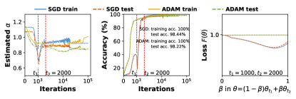
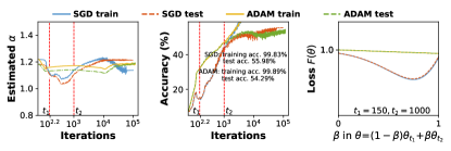
(a) MNIST	(b) CIFAR10

Figure 4: Behaviors illustration of Sgd and Adam on fully connected networks. In both (a) and (b), the left and middle figures respectively report the estimated tail index $\alpha$ in $\mathcal{S}\alpha\mathcal{S}$ distribution and classification accuracies; right figures show possible barriers between the solutions $\bm{\theta}_{1000}$ and $\bm{\theta}_{2000}$ on MNIST, and $\bm{\theta}_{150}$ and $\bm{\theta}_{1000}$ on CIFAR10, respectively. Best viewed in $\times$2 sized color pdf file.

5 Experiments

In this section, we first investigate the gradient noise in Adam and Sgd, and then show their iteration-based convergence behaviors to testify the implications of our escaping theory. The code is available at https://panzhous.github.io.

Heavy Tails of Gradient Noise. We respectively use Sgd and Adam to train AlexNet [52] on CIFAR10, and show the statistical behaviors of gradient noise on CIFAR10. To fit the noise via $\mathcal{S}\alpha\mathcal{S}$ distribution, we consider covariance matrix $\bm{\Sigma}_{t}$ and use the approach in [23, 53] to estimate the tail index $\alpha$. Fig. 1 in Sec. 1 and Fig. 5 in Appendix B show that the gradient noise in both Sgd and Adam usually reveal the heavy tails and can be well characterized by $\mathcal{S}\alpha\mathcal{S}$ distribution. This testifies the heavy tail assumption on the gradient noise in our theories.

Escaping Behaviors. We investigate the iteration-based convergence behaviors of Sgd and Adam, including their training and test accuracies and losses and tail index of their gradient noise. For MNIST [54] and CIFAR10 [55], we respectively use nine- and seven-layered fully-connected-networks. Each layer has 512 neurons and contains a linear layer and a ReLu layer. Firstly, the results in the middle figures show that Sgd usually has better generalization performance than Adam-alike adaptive algorithms which is consistent with the results in [17, 12, 30, 18].

Moreover, from the trajectories of the tail index $\alpha$ and accuracy of Sgd on MNIST and CIFAR10 in Fig. 4, one can observe two distinct phases. Specifically, for the first 1000 iterations in MNIST and 150 iterations in CIFAR10, both the training and test accuracies increase tardily, while the tail index parameter $\alpha$ reduces quickly. This process continues until $\alpha$ reaches its lowest value. When considering the barrier around inflection point (e.g. a barrier between $\bm{\theta}_{1000}$ and $\bm{\theta}_{2000}$ on MNIST), it seems that the process of Sgd has a sudden jump from one basin to another one which leads to a sudden accuracy drop, and then gradually converges. Accordingly, the accuracies are improved quickly. In contrast, one cannot observe similar phenomenon in Adam. This is because as our theory suggested, Sgd is more locally unstable and converges to flatter minima than Adam, which is caused by the geometry adaptation, exponential gradient average and smaller learning rate in Adam. All these results are consistent with our theories and also explain the well observed evidences in [12, 30, 31, 51, 17] that Sgd usually converges to flat minima which often locate at the flat or asymmetric basins/valleys, while Adam does not. Because the empirical observations [1, 19, 20, 21] show that minima at the flat or asymmetric basins/valleys often generalize better than sharp ones, our empirical and theoretical results can well explain the generalization gap between Adam-alike algorithms and Sgd.

6 Conclusion

In this work, we analyzed the generalization performance degeneration of Adam-alike adaptive algorithms over Sgd. By looking into the local convergence behaviors of the Lévy-driven SDEs of these algorithms through analyzing their escaping time, we prove that for the same basin, Sgd has smaller escaping time than Adam and tends to converge to flatter minima whose local basins have larger Radon measure, explaining its better generalization performance. This result is also consistent with the widely observed convergence behaviors of Sgd and Adam in many literatures. Finally our experimental results testify the heavy gradient noise assumption and implications in our theory.

Broader Impacts

This work theoretically analyzes a fundamental problem in deep learning field, namely the generalization gap between adaptive gradient algorithms and Sgd, and reveals the essential reasons for the generalization degeneration of adaptive algorithms. The established theoretical understanding of these algorithms may inspire new algorithms with both fast convergence speed and good generalization performance, which alleviate the need for computational resource and achieve state-of-the-art results. Yet it still needs more efforts to provide more insights to design practical algorithms.

Appendix A Structure of This Document

This supplementary document contains the technical proofs of convergence results and some additional numerical results of the main draft entitled “Towards Theoretically Understanding Why Sgd Generalizes Better Than Adam in Deep Learning”. It is structured as follows. In Appendix B, we provides more construction details of the SDE for Adam and also conduct experiments which show very similar convergence behaviors of Adam (Sgd) and its SDE. Appendix C compares our work with the related work [32, 33] in more details. Appendix D summarizes the notations throughout this document and also provides the auxiliary theories and lemmas for subsequent analysis whose proofs are deferred to Appendix F. Then Appendix E gives the proofs of the main results in Sec. 4, including Theorem 1 which analyzes the escaping time analysis of Lévy-driven SDEs and Theorem 2 which proves the processes with and without Lévy motion are close to each other. Finally, in Appendix F we presents the proofs of auxiliary theories and lemmas in Appendix D, including Theorems 3 $\sim$ 4 and Lemmas 1 $\sim$ 3.

Appendix B More Discussion of SDE in Adam

Here we provide more discussion and construction details for the SDE in Adam. We first investigate the second order moment of the gradient noise in Adam. Then we introduce the two types of randomness in the SDE of Adam. Finally, we run experiments to investigate the validity of the constructed SDEs of Adam and Sgd.

B.1 $\mathcal{S}\alpha\mathcal{S}$-distributed Gradient Noise in Adam

In the manuscript, we have shown the gradient noise itself to be $\mathcal{S}\alpha\mathcal{S}$-distributed. Here we further investigate the second-order moment of the gradient noise. From the bottom row of Figure 5, one can observe that (1) both the second-order moment of the gradient noise also reveals heavy tails; (2) compared with Gaussian distribution, $\mathcal{S}\alpha\mathcal{S}$ distribution can better characterize this kind of second-order moment of the gradient noise. All these results demonstrate that the gradient noise in both Adam and Sgd actually satisfies the $\mathcal{S}\alpha\mathcal{S}$ distribution. So the heavy-tailed gradient noise assumptions in our manuscript is very reasonable.

B.2 Randomness in SDE of Adam

The SDE of ADAM approximates gradient noise $\bm{m}_{t}$ via the combination of full gradient and Lévy motion but does not approximate $\bm{v}_{t}$. This SDE should be more accurate than the one which approximates both $\bm{m}_{t}$ and the coefficients $\bm{v}_{t}$. So the randomness in the SDE of Adam comes from the Lévy motion and also $\bm{v}_{t}$ caused by sampling a minibatch. But these two types of randomness actually do not depend on each other. Note that as shown in many literatures, e.g. [56, 57], SDE allows randomness in coefficients and also enjoys many good properties, such as stability and unique solution. This type of SDE is usually called “SDE with random coefficients", and usually appears in stochastic jump systems [58], economics and finance [59, 60], biology [61, 62], mechanics and physics [63], etc. See more details of SDE with random coefficients in [56, 57].

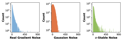
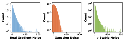
(a) Gradient noise in Adam	(b) Gradient noise in Sgd
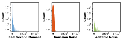
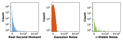
(c) Second-order moment of gradient noise in Adam	(d) Second-order moment of gradient noise in Sgd

Figure 5: Illustration of gradient noise in Adam and Sgd. The left figures in (a) and (b) are the real gradient noise computed with AlexNet on CIFAR10. Similarly, the left figures in (c) and (d) are the second-order moment of gradient noise computed with AlexNet on CIFAR10. The middle and right figures in (a) $\sim$ (d) are respectively the fitted Gaussian and systemic $\alpha$-stable noise. By comparison, $\alpha$-stable noise can better characterize real gradient noise in deep learning.

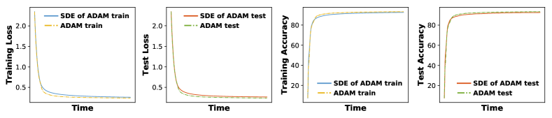
(a) Adam

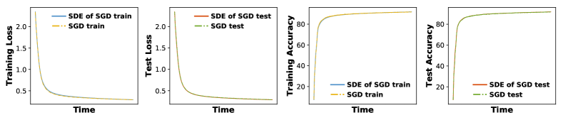
(b) Sgd

Figure 6: Illustration of convergence trajectories of Adam, Sgd and their SDEs. One can observe that for Adam, it convergence trajectories are very similar to its SDE, which shows the validity of the SDE construction. Similarly, we can observe the same observations on Sgd and its SDE.

B.3 Convergence Behavior Comparison between Algorithm and Its SDE

Here we conduct experiments on 784-10-10-sized networks and report the convergence behvariors of Adam (Sgd) and its SDE in Fig. 6. Note SDE actually equals to injecting heavy tailed noise into Sgd and Adam that use full gradients. We use a relatively small network since simulating high-dimensional gradient noise $\bm{u}_{t}$ and computing the huge covariance matrix $\bm{\Sigma}_{t}$ at each iteration are too computationally expensive to compute. From the convergence trajectories of both Adam and its SDE in Fig. 6 (a), one can observe that they have very similar convergence behaviors. Similarly, in Fig. 6 (b) we can observe the same observations on Sgd and its SDE. So injecting heavy tailed noise into Sgd and Adam that use full gradients leads to similar convergence behaviors to Sgd and Adam that use stochastic gradients. These results well demonstrate the validity of current SDE construction. Note that here we do not observe jump behaviors, since the networks are very small and may have not very sharp minima. But these results as aforementioned can testify the validity of current SDE construction.

Appendix C Comparison to Related Works

Dinh et al. [32] showed flat minimum can become sharp by scaling two layers at the same time. But with this scaling, sharp minimum cannot be arbitrarily flat, as if the eigenvalues of two parameters in the same layer has large ratio, this scaling cannot change this ratio. So flat and sharp minimum are not totally equivalent. Combining the observation in many works that flat minima could achieve better generalization performance than sharper ones, one could conclude that flat minima can generalize well in most case, while sharp minima that can become flat one by linearly scaling two layers also can generalize but other sharp minima cannot. So analyzing the flat and sharp properties is still meaningful. Besides, the flatness in this work is defined on general non-zero Radon measure. If one finds an invariant measure to the scaling in [32], the flatness is also invariant, providing more insights to generalization. So it is promising to explore this invariant measure in the future.

Appendix D Notations and Auxiliary Lemmas

D.1 Notations

For analyzing the uniform Lévy-driven SDEs in Eqn. (4) and (5), we first decompose the Lévyprocess $L_{t}$ into two components $\bm{\xi}_{t}$ and $\bm{\zeta}_{t}$, namely

$$L_{t}=\bm{\xi}_{t}+\bm{\zeta}_{t}$$ (10)

whose characteristic functions are respectively defined as

$$\begin{split}\mathbb{E}[e^{i\langle\bm{\lambda},\bm{\xi}_{t}\rangle}]=&e^{t{\int}_{{\mathbb{R}^{d}}\!\setminus\!\{\bm{0}\}}\zeta\mathbb{I}\left\{\|\bm{y}\|\leq\frac{1}{{\varepsilon^{\delta}}}\right\}\nu(\textsf{d}\bm{y})},\\ \mathbb{E}[e^{i\langle\bm{\lambda},\bm{\zeta}_{t}\rangle}]=&e^{t{\int}_{{\mathbb{R}^{d}}\!\setminus\!\{\bm{0}\}}\zeta\mathbb{I}\left\{\|\bm{y}\|\geq\frac{1}{{\varepsilon^{\delta}}}\right\}\nu(\textsf{d}\bm{y})},\end{split}$$

where $\zeta=e^{i\langle\bm{\lambda},\bm{y}\rangle}-1-i\langle\bm{\lambda},\bm{y}\rangle\mathbb{I}\left\{\|\bm{y}\|\leq 1\right\}$, ${\varepsilon}$ (in Eqn. (4) and (5)) and $\delta$ are two small constants satisfying ${\varepsilon^{-\delta}}<1$ and will be specified later. Define the Lévy measures $\nu$ as $\nu(\textsf{d}\bm{y})=\frac{1}{\|\bm{y}\|^{1+\alpha}}\textsf{d}\bm{y}$. Accordingly, the Lévy measures $\nu$ of the stochastic processes $\bm{\xi}$ and $\bm{\zeta}$ are

$$\nu_{\bm{\xi}}=\nu\big{(}\bm{A}\cap\{0<\|\bm{y}\|\leq\frac{1}{{\varepsilon^{\delta}}}\}\big{)},\ \nu_{\bm{\zeta}}=\nu\big{(}\bm{A}\cap\{\|\bm{y}\|\geq\frac{1}{{\varepsilon^{\delta}}}\}\big{)},$$

where $\bm{A}\in\mathcal{B}({\mathbb{R}^{d}})$. In this way, the stochastic process $\bm{\xi}$ has infinite Lévy measure with support $\{\bm{y}\ |\ 0<\|\bm{y}\|\leq{\varepsilon^{-\delta}}\}$ and thus makes infinitely many jumps on any time interval. But the jump size does not exceed ${\varepsilon^{-\delta}}$ and thus is small which actually does not help escape the current local basin. In contrast, the Lévy measure $\nu_{\bm{\zeta}}(\cdot)$ of $\bm{\zeta}$ is finite and is computed as

$$\Theta({\varepsilon}^{-\delta})=\int_{\|\bm{y}\|\geq{\varepsilon^{-\delta}}}\nu(\textsf{d}\bm{y})={\int}_{\|\bm{y}\|\geq{\varepsilon^{-\delta}}}\frac{\textsf{d}\bm{y}}{\|\bm{y}\|^{1+\alpha}}=\frac{2}{\alpha}{\varepsilon^{\alpha\delta}}.$$

So the process $\bm{\zeta}$ is a compound Poisson process with intensity $\Theta({\varepsilon}^{-\delta})$ and jumps distributed according to the law of $1/\Theta({\varepsilon}^{-\delta})$. Specifically, let $0=t_{1}<t_{2}\cdots<t_{k}<\cdots$ denote the times of successive jumps of $\bm{\zeta}$ and $J_{k}$ denote the jump size at the $k$-th jump. Then the inner-jump times $\sigma_{k}=t_{k}-t_{k-1}$ are i.i.d. exponentially distributed random variables with mean value $\mathbb{E}(\sigma_{k})=\frac{1}{\Theta({\varepsilon}^{-\delta})}$ and the probability distribution function $\mathbb{P}\left(\sigma_{k}\leq x\right)=1-\exp(-x\Theta({\varepsilon}^{-\delta}))$. The probability law of $J_{k}$ is also known explicitly in terms of the Lévy measure $\nu$:

$$\mathbb{P}\left(J_{k}\!\in\!\bm{A}\right)\!=\!\frac{1}{\Theta({\varepsilon}^{-\delta})}\nu\!\left(\bm{A}\!\cap\!\{\bm{y}\!\ |\ \!\|\bm{y}\|\geq{\varepsilon^{-\delta}}\}\right)\!,\ \bm{A}\!\in\!\mathcal{B}({\mathbb{R}^{d}}).$$

So the main force for escaping the local basin comes from the big jumps in the process $\bm{\zeta}$ which will be rigorous analyzed in the following sections.

Besides, for analysis, we usually need to consider affects of the Lévy motion (noise) $L_{t}$ to the Lévy-driven SDEs of Sgd and Adam given in Eqn. (4) and (5). So here we define two Lévy-free SDEs which respectively correspond to Eqn. (4) and (5):

$$\textsf{d}\widehat{\bm{\theta}}_{t}=\nabla\bm{F}(\widehat{\bm{\theta}}_{t}),$$ (11)

and

$$\begin{cases}\textsf{d}\widehat{\bm{\theta}}_{t}=&-\mu_{t}\widehat{\bm{Q}}_{t}^{-1}\widehat{\bm{m}}_{t},\\ \textsf{d}\widehat{\bm{m}}_{t}=&\beta_{1}(\nabla\bm{F}(\widehat{\bm{\theta}}_{t})-\widehat{\bm{m}}_{t})\\ \textsf{d}\widehat{\bm{v}}_{t}=&\beta_{2}(\nabla f_{\mathcal{S}_{t}}(\widehat{\bm{\theta}}_{t})^{2}-\widehat{\bm{v}}_{t}).\\ \end{cases}$$ (12)

where $\widehat{\bm{Q}}_{t}=\operatorname{diag}\left(\sqrt{\widehat{\bm{v}}_{t}}+\epsilon\right)$. Then by analyzing the distance $\|\widehat{\bm{\theta}}_{t}-\bm{\theta}_{t}\|$ between the processes $\widehat{\bm{\theta}}_{t}$ without Lévy motion and $\bm{\theta}_{t}$ with Lévy motion, we can well know the effects of the Lévy motion to the escaping behaviors.

D.2 Auxiliary Theories and Lemmas

Theorem 3.

Suppose Assumptions 1 and 2 holds. Then for Lévy-driven Sgd SDE (11) with $\widehat{\bm{Q}}_{t}=\bm{I}$ and $\beta_{2}=0$, the Lyapunov function $\mathcal{L}(t)=\bm{F}(\widehat{\bm{\theta}}_{t})-\bm{F}(\bm{\theta}^{*})$ obeys

$$\begin{split}\mathcal{L}(t)\leq\Delta\exp\left(-2\mu t\right)\end{split}$$

where $\Delta=\bm{F}(\widehat{\bm{\theta}}_{0})-\bm{F}(\bm{\theta}^{*})$ with the optimum solution $\bm{\theta}^{*}$ in the current local basin $\bm{\Omega}$. The sequence $\{\widehat{\bm{\theta}}_{t}\}$ produced by Eqn. (11) obeys

$$\begin{split}\|\widehat{\bm{\theta}}_{t}-\bm{\theta}^{*}\|_{2}^{2}\leq\frac{2\Delta}{\mu}\exp\left(-2\mu t\right).\end{split}$$

See its proof in Appendix F.1.

Theorem 4.

Suppose Assumptions 1 and 2 holds. Assume the sequence $\{(\widehat{\bm{\theta}}_{t},\widehat{\bm{m}}_{t},\widehat{\bm{v}}_{t})\}$ are produced by Eqn. (12). Let $\widehat{\bm{s}}_{t}=\frac{h_{t}}{\mu_{t}}\left(\sqrt{\omega_{t}\widehat{\bm{v}}_{t}}+\epsilon\right)$ with $h_{t}=\beta_{1}$, $\mu_{t}=(1-e^{-\beta_{1}t})^{-1}$ and $\omega_{t}=(1-e^{-\beta_{2}t})^{-1}$. We define $\|\bm{x}\|_{\bm{y}}^{2}=\sum_{i}\bm{y}_{i}\bm{x}_{i}^{2}$. Then for Lévy-driven Adam SDEs in Eqn. (12), its Lyapunov function $\mathcal{L}(t)=\bm{F}(\widehat{\bm{\theta}}_{t})-\bm{F}(\bm{\theta}^{*})+\frac{1}{2}\|\widehat{\bm{m}}_{t}\|_{\widehat{\bm{s}}_{t}^{-1}}$ with the optimum solution $\bm{\theta}^{*}$ in the current local basin $\bm{\Omega}$ obeys

$$\begin{split}\mathcal{L}(t)\leq\Delta\exp\left(-\frac{2\mu\tau}{\beta_{1}\left(v_{\max}+\epsilon\right)+\mu\tau}\left(\beta_{1}-\frac{\beta_{2}}{4}\right)t\right)\end{split}$$

where $\Delta=\bm{F}(\widehat{\bm{\theta}}_{0})-\bm{F}(\bm{\theta}^{*})$ due to $\widehat{\bm{m}}_{0}=\bm{0}$. The sequence $\{\widehat{\bm{\theta}}_{t}\}$ produced by Eqn. (12) obeys

$$\begin{split}\|\widehat{\bm{\theta}}_{t}-\bm{\theta}^{*}\|_{2}^{2}\leq\frac{2\Delta}{\mu}\exp\left(-\frac{2\mu\tau}{\beta_{1}\left(v_{\max}+\epsilon\right)+\mu\tau}\left(\beta_{1}-\frac{\beta_{2}}{4}\right)t\right).\end{split}$$

See its proof in Appendix F.2.

Lemma 1.

(1) The process $\bm{\xi}$ in Eqn. (10) can be decomposed into two processes $\widehat{\bm{\xi}}$ and linear drift, namely,

$$\bm{\xi}_{t}=\widehat{\bm{\xi}}_{t}+\mu_{\varepsilon}t,$$ (13)

where $\widehat{\bm{\xi}}$ is a zero mean Lévymartingale with bounded jumps.
(2) Let $\delta\in(0,1)$, $\mu_{\varepsilon}=\mathbb{E}[\bm{\xi}_{1}]$ and $T_{\varepsilon}={\varepsilon^{-\theta}}$ for some $\theta>0$, $\rho_{0}=\rho_{0}(\delta)=\frac{1-\delta}{4}>0$ and $\theta_{0}=\theta_{0}(\delta)=\frac{1-\delta}{3}>0$. Suppose ${\varepsilon}$ is sufficient small such that such that $\Theta(1)\leq{\varepsilon^{-\frac{1-\delta}{6}}}$ and ${\varepsilon^{-\rho}}-2(C+\Theta(1)){\varepsilon^{\frac{7}{6}(1-\delta)+\frac{\rho}{2}}}\geq 1$ with a constant $C=\left|\int_{0<u\leq 1}u^{2}\textsf{d}\Theta(u)\right|\in(0,+\infty)$. Then for all $\delta\in(0,\delta_{0})$, $\theta\in(0,\theta_{0})$ there are $p_{0}=p_{0}(\delta)=\frac{\delta}{2}$ and ${\varepsilon}_{0}={\varepsilon}_{0}(\delta,\rho)$ such that the estimates

$$\|{\varepsilon}\bm{\xi}_{T_{\varepsilon}}\|={\varepsilon}\|\mu_{\varepsilon}\|T_{\varepsilon}<{\varepsilon^{2\rho}}\quad\text{and}\quad\mathbb{P}\left([{\varepsilon}\bm{\xi}]_{T_{\varepsilon}}^{d}\geq{\varepsilon^{\rho}}\right)\leq\exp(-{\varepsilon^{-p}})$$

hold for all $p\in(0,p_{0}]$ and ${\varepsilon}\in(0,{\varepsilon}_{0}]$.

See its proof in Appendix F.3.

Lemma 2.

Let $\delta\in(0,1)$ and $\bm{g}^{t}_{t\geq 0}$ be a bounded adapted cȧdlȧg stochastic process with values in ${\mathbb{R}^{d}}$, $T_{\varepsilon}={\varepsilon^{-\theta}}$, $\theta>0$. Suppose $\sup_{t\geq 0}\|\bm{g}^{t}\|$ is well bounded. Assume $\rho_{0}=\rho_{0}(\delta)=\frac{1-\delta}{16}>0$, $\theta_{0}=\theta_{0}(\delta)=\frac{1-\delta}{3}>0$, $p_{0}=\frac{\rho}{2}$. For $\widehat{\bm{\xi}}_{t}$ in Eqn. (13), there is $\delta_{0}=\delta_{0}(\delta)>0$ such that for all $\rho\in(0,\rho_{0})$ and $\theta\in(0,\theta_{0})$, it holds

$$\mathbb{P}\left(\sup_{0\leq t\leq T_{\varepsilon}}\epsilon\left|\sum_{i=1}^{d}\int_{0}^{t}\bm{g}_{s-}^{i}\textsf{d}\widehat{\bm{\xi}}_{s}^{i}\right|\geq{\varepsilon^{\rho}}\right)\leq 2\exp\left(-{\varepsilon^{-p}}\right)$$

for all $p\in(0,p_{0}]$ and $0<{\varepsilon}\leq{\varepsilon}_{0}$ with $\epsilon_{0}={\varepsilon}_{0}(\rho)$, where $\widehat{\bm{\xi}}_{s}^{i}$ denotes the $i$-th entry in $\widehat{\bm{\xi}}_{s}$.

See its proof of Appendix F.4.

Lemma 3.

Suppose Assumptions 1 and 2 holds. Assume $\delta\in(0,1)$, $\rho_{0}=\rho_{0}(\delta)=\frac{1-\delta}{16(1+c_{1}\kappa_{1})}>0$, $\theta_{0}=\theta_{0}(\delta)=\frac{1-\delta}{3}>0$, $p_{0}=\min(\frac{\bar{\rho}(1+c_{1}\kappa_{1})}{2},p)$, $\frac{1}{c_{2}}\ln\left(\frac{2\Delta}{\mu{\varepsilon^{\bar{\rho}}}}\right)\leq{\varepsilon^{-\theta_{0}}}$ where $\kappa_{1}=\ell$ and $c_{2}=2\mu$ in Sgd, $\kappa_{1}=\frac{c_{2}\ell}{(v_{\min}+\epsilon)|\tau_{m}-1|}$ and $c_{3}=\frac{2\mu\tau}{\beta_{1}\left(v_{\max}+\epsilon\right)+\mu\tau}\big{(}\beta_{1}-\frac{\beta_{2}}{4}\big{)}$ in Adam. Here $c_{1}$ $\sim$ $c_{3}$ are positive constants. For all $\bar{\rho}\in(0,\rho_{0})$, $p\in(0,p_{0}]$, $0<{\varepsilon}\leq{\varepsilon}_{0}$ with ${\varepsilon}_{0}={\varepsilon}_{0}(\bar{\rho})$, and $\bm{\theta}_{0}=\widehat{\bm{\theta}}_{0}$, we have

$$\sup_{\bm{\theta}_{0}\in\bm{\Omega}}\mathbb{P}\left(\sup_{0\leq t<\sigma_{1}}\|\bm{\theta}_{t}-\widehat{\bm{\theta}}_{t}\|\geq 2{\varepsilon^{\bar{\rho}}}\right)\leq 2\exp(-{\varepsilon^{-p/2}}),$$ (14)

where the sequences $\bm{\theta}_{t}$ and $\widehat{\bm{\theta}}_{t}$ are respectively produced by Eqn. (5) and (12) in Adam or Eqn. (4) and (11) in RMSProp and Sgd.

See its proof in Appendix F.5.

Appendix E Proof of Results in Sec. 4

E.1 Proof of Theorem 1

Proof.

Here we first briefly introduce our proof idea. As we proved in Lemma 3, for any $\delta\in(0,1)$, there exist $\rho_{0}$, $p_{0}$ and ${\varepsilon}_{0}$ such that for all $\bar{\rho}\in(0,\rho_{0})$, $p\in(0,p_{0}]$ and $0<{\varepsilon}\leq{\varepsilon}_{0}$, we have

$$\sup_{\bm{\theta}_{0}\in\bm{\Omega}}\mathbb{P}\left(\sup_{0\leq t<\sigma_{1}}\|\bm{\theta}_{t}-\widehat{\bm{\theta}}_{t}\|\geq 2{\varepsilon^{\bar{\rho}}}\right)\leq 2\exp(-{\varepsilon^{-p/2}}),$$ (15)

where the sequences $\bm{\theta}_{t}$ and $\widehat{\bm{\theta}}_{t}$ share the same initialization $\bm{\theta}_{0}=\widehat{\bm{\theta}}_{0}$. Such a result holds for both Sgd and Adam. Besides, from Theorems 3 and 4, we know that the sequence $\{\widehat{\bm{\theta}}_{t}\}$ produced by Eqn. (11) or (12) (namely, the dynamic systems of Sgd and Adam) exponentially converges to the minimum $\bm{\theta}^{*}$ of the current local basin $\bm{\Omega}$. To escape the local basin $\bm{\Omega}$, there are two possible choices, the small jumps in the process $\bm{\xi}$ and the big jumps $J_{k}$ in the process $\bm{\zeta}$. As the small jumps in the process $\bm{\xi}$ is well bounded, it is not very likely that these small jumps can help escape the local basin $\bm{\Omega}$ which is verified by Eqn. (15). We well prove this more rigorously latter. For the big jumps $J$, since the expectation jump time $\mathbb{E}(\sigma_{1})$ is $1/\Theta({\varepsilon}^{-\delta})$, such as $\mathbb{E}(\sigma_{1})=\frac{2}{\alpha}{\varepsilon^{\alpha\delta}}$ in the $\alpha$-stable ($\mathcal{S}\alpha\mathcal{S}$) distribution, $\mathbb{E}(\sigma_{1})$ is usually much larger than the necessary time $t=\mathcal{O}(\ln(1/{\varepsilon}))$ to achieve $\|\widehat{\bm{\theta}}_{t}-\bm{\theta}^{*}\|\leq{\varepsilon^{\delta}}$. This means that before the jump time $\sigma_{1}$ the sequence $\widehat{\bm{\theta}}_{t}$ is very close to the optimum of $\bm{\Omega}$ and thus $\bm{\theta}_{t}$ is very close to the minimum $\bm{\theta}^{*}$. In this way, the escaping time $\Gamma$ of the sequence $\{\bm{\theta}_{t}\}$ most likely occurs at the time $\sigma_{1}$ if the big jump ${\varepsilon}J_{1}$ in the process $\bm{\zeta}$ is large. If the jump ${\varepsilon}J_{1}$ is small and $\bm{\theta}_{\sigma_{1}}$ does not escape $\bm{\Omega}$, then $\bm{\theta}_{t}$ will converge to the minimum $\bm{\theta}^{*}$ exponentially and stay in the small neighborhood of $\bm{\theta}^{*}$. Accordingly, before the second jump time $t_{2}=t_{1}+\sigma_{2}$, $\bm{\theta}_{t_{2}}$ will jump. This process will continue during the time interval $[0,t]$. Since for each jump time $t_{k}-$, $\bm{\theta}_{t_{k}-}$ is very close to the optimum $\bm{\theta}^{*}$, the big jump size ${\varepsilon}\bm{Q}_{t_{k}}^{-1}\bm{\Sigma}_{t_{k}}J_{t_{k}}\approx{\varepsilon}\bm{Q}_{\bm{\theta}^{*}}^{-1}\bm{\Sigma}_{\bm{\theta}^{*}}J_{t_{k}}$. So we can use ${\varepsilon}\bm{Q}_{t}^{-1}\bm{\Sigma}_{t}J_{t_{k}}\approx{\varepsilon}\bm{Q}_{\bm{\theta}^{*}}^{-1}\bm{\Sigma}_{\bm{\theta}^{*}}J_{t_{k}}\notin\bm{\Omega}$ to judge whether at time $t_{k}$, $\bm{\theta}_{t_{k}}$ escapes the local basin $\bm{\Omega}$. The events $\{{\varepsilon}J_{1}\notin\bm{\mathcal{W}}\}=\{{\varepsilon}\bm{Q}_{\bm{\theta}^{*}}^{-1}\bm{\Sigma}_{\bm{\theta}^{*}}J_{t_{k}}\notin\bm{\Omega}\}$, $\cdots$, $\{{\varepsilon}J_{k-1}\notin\bm{\mathcal{W}}\}=\{{\varepsilon}\bm{Q}_{\bm{\theta}^{*}}^{-1}\bm{\Sigma}_{\bm{\theta}^{*}}J_{t_{k-}}\notin\bm{\Omega}\}$, $\{{\varepsilon}J_{k}\notin\bm{\mathcal{W}}\}=\{{\varepsilon}\bm{Q}_{\bm{\theta}^{*}}^{-1}\bm{\Sigma}_{\bm{\theta}^{*}}J_{t_{k}}\notin\bm{\Omega}\}$ are independent.

Now we prove the desired results from two aspects, namely establishing upper bound and lower bound of $\mathbb{E}\left[\exp\left(-um(\bm{\mathcal{W}})\Theta({\varepsilon^{-1}})\Gamma\right)\right]$ for any $u>-1$. Before that, we first establish basic inequalities for lower and upper bounds.

Basic inequalities for lower and upper bounds. Since $\sigma_{1}$ is exponentially distributed with the parameter $\Theta(\epsilon^{-\delta})$, we compute the Laplace transform of $m(\bm{\mathcal{W}})\Theta({\varepsilon^{-1}})\sigma_{1}$ as follows:

$$\begin{split}&\mathbb{E}\left[e^{-um(\bm{\mathcal{W}})\Theta({\varepsilon^{-1}})\sigma_{1}}\right]=\mathbb{E}\left[\int_{0}^{+\infty}e^{-um(\bm{\mathcal{W}})\Theta({\varepsilon^{-1}})\sigma_{1}}\cdot\Theta({\varepsilon}^{-\delta})e^{-\Theta({\varepsilon}^{-\delta})\sigma_{1}}\textsf{d}\sigma_{1}\right]\\ =&\frac{\Theta({\varepsilon}^{-\delta})}{\Theta({\varepsilon}^{-\delta})+um(\bm{\mathcal{W}})\Theta({\varepsilon^{-1}})}=\frac{1}{1+ua_{\varepsilon}},\end{split}$$

where $a_{\varepsilon}=m(\bm{\mathcal{W}})\frac{\Theta({\varepsilon^{-1}})}{\Theta(-{\varepsilon^{\delta}})}\ \text{and}\ \Theta({\varepsilon}^{-\delta})=\Theta(-{\varepsilon^{\delta}}).$ Besides, for the probability law of the big jump we have

$$\mathbb{P}\left(\bm{Q}_{\bm{\theta}^{*}}^{-1}\bm{\Sigma}_{\bm{\theta}^{*}}{\varepsilon}J_{1}\notin\bm{\Omega}\right)=\mathbb{P}\left({\varepsilon}J_{1}\in\bm{\mathcal{W}}\right)=\frac{\nu(\bm{\mathcal{W}}/{\varepsilon})}{\Theta({\varepsilon}^{-\delta})}.$$

Since for the Lévy measure, we have $m(\bm{\mathcal{W}})=\lim_{u\rightarrow+\infty}\frac{\nu(u\bm{\mathcal{W}})}{\Theta(u)}$ according to [29]. So for any $\delta^{\prime}$, there always exists ${\varepsilon}$ such that it holds

$$a_{\varepsilon}(1-\delta^{\prime})\leq\frac{\nu(\bm{\mathcal{W}}/{\varepsilon})}{\Theta({\varepsilon}^{-\delta})}=\frac{\nu(\bm{\mathcal{W}}/{\varepsilon})}{\Theta({\varepsilon^{-1}})}\frac{\Theta({\varepsilon^{-1}})}{\Theta({\varepsilon}^{-\delta})}\overset{\text{\char 172}}{\approx}m(\bm{\mathcal{W}})\frac{\Theta({\varepsilon^{-1}})}{\Theta({\varepsilon}^{-\delta})}=m(\bm{\mathcal{W}})\frac{\Theta({\varepsilon^{-1}})}{\Theta({\varepsilon^{-\delta}})}\leq a_{\varepsilon}(1+\delta^{\prime}).$$ (16)

where ① holds since ${\varepsilon}$ is enough small. Then with the help of the continuity of the function $(\bm{\theta},\bm{z})\rightarrow\bm{Q}_{\bm{\theta}}^{-1}\bm{\Sigma}_{\bm{\theta}}\bm{z}$ both in $\bm{\theta}$ and $\bm{z}$. Indeed, for any $\delta^{\prime}$ we can choose $R>0$ enough large such that for small ${\varepsilon}$ we have

$$\mathbb{P}\left(\|{\varepsilon}J_{1}\|>R\right)\leq\frac{\delta^{\prime}}{4}\frac{\Theta({\varepsilon^{-1}})}{\Theta({\varepsilon^{-\delta}})}.$$

Further, the function $(\bm{\theta},\bm{z})\rightarrow\bm{Q}_{\bm{\theta}}^{-1}\bm{\Sigma}_{\bm{\theta}}\bm{z}$ is uniformly continuous in $\bm{z}$ in the ball $\|\bm{z}\|\leq R$ and is continuous in $\bm{\theta}$ at the optimum $\bm{\theta}^{*}$. Following [29], by using the scaling property of the jump measure $\nu$ and the fact that the limiting measure $m$ has no atoms we show that uniformly over $\|\bm{\theta}-\bm{\theta}^{*}\|\leq{\varepsilon^{\gamma}}$:

$$\begin{cases}\left|\mathbb{P}\left(\bm{Q}_{\bm{\theta}}^{-1}\bm{\Sigma}_{\bm{\theta}}{\varepsilon}J_{k}\notin\bm{\Omega}^{\pm{\varepsilon^{\gamma}}},\ \|{\varepsilon}J_{k}\|\leq R\right)-\mathbb{P}\left(\bm{Q}_{\bm{\theta}^{*}}^{-1}\bm{\Sigma}_{\bm{\theta}^{*}}{\varepsilon}J_{k}\notin\bm{\Omega},\ \|{\varepsilon}J_{k}\|\leq R\right)\right|\leq\frac{\delta^{\prime}}{4}\frac{\Theta({\varepsilon^{-1}})}{\Theta({\varepsilon^{-\delta}})},\\ \left|\mathbb{P}\left(\bm{Q}_{\bm{\theta}}^{-1}\bm{\Sigma}_{\bm{\theta}}{\varepsilon}J_{k}\notin\bm{\Omega},\ \|{\varepsilon}J_{k}\|\leq R\right)-\mathbb{P}\left(\bm{Q}_{\bm{\theta}^{*}}^{-1}\bm{\Sigma}_{\bm{\theta}^{*}}{\varepsilon}J_{k}\notin\bm{\Omega},\ \|{\varepsilon}J_{k}\|\leq R\right)\right|\leq\frac{\delta^{\prime}}{4}\frac{\Theta({\varepsilon^{-1}})}{\Theta({\varepsilon^{-\delta}})},\\ \end{cases}$$ (17)

At the same time, we also can establish

$$\begin{split}&\mathbb{P}\left(\bm{Q}_{\bm{\theta}^{*}}^{-1}\bm{\Sigma}_{\bm{\theta}^{*}}{\varepsilon}J_{k}\notin\bm{\Omega}\right)-\mathbb{P}\left(\bm{Q}_{\bm{\theta}^{*}}^{-1}\bm{\Sigma}_{\bm{\theta}^{*}}{\varepsilon}J_{k}\notin\bm{\Omega},\ \|{\varepsilon}J_{k}\|\leq R\right)\\ =&\mathbb{P}\left(\bm{Q}_{\bm{\theta}^{*}}^{-1}\bm{\Sigma}_{\bm{\theta}^{*}}{\varepsilon}J_{k}\notin\bm{\Omega}\right)-\mathbb{P}\left(\|{\varepsilon}J_{k}\|\leq R\ |\ \bm{Q}_{\bm{\theta}^{*}}^{-1}\bm{\Sigma}_{\bm{\theta}^{*}}{\varepsilon}J_{k}\notin\bm{\Omega}\right)\mathbb{P}\left(\bm{Q}_{\bm{\theta}^{*}}^{-1}\bm{\Sigma}_{\bm{\theta}^{*}}{\varepsilon}J_{k}\notin\bm{\Omega}\right)\\ =&\mathbb{P}\left(\bm{Q}_{\bm{\theta}^{*}}^{-1}\bm{\Sigma}_{\bm{\theta}^{*}}{\varepsilon}J_{k}\notin\bm{\Omega}\right)(1-\mathbb{P}\left(\|{\varepsilon}J_{k}\|\leq R\ |\ \bm{Q}_{\bm{\theta}^{*}}^{-1}\bm{\Sigma}_{\bm{\theta}^{*}}{\varepsilon}J_{k}\notin\bm{\Omega}\right))\\ =&\mathbb{P}\left(\bm{Q}_{\bm{\theta}^{*}}^{-1}\bm{\Sigma}_{\bm{\theta}^{*}}{\varepsilon}J_{k}\notin\bm{\Omega}\right)\mathbb{P}\left(\|{\varepsilon}J_{k}\|>R\ |\ \bm{Q}_{\bm{\theta}^{*}}^{-1}\bm{\Sigma}_{\bm{\theta}^{*}}{\varepsilon}J_{k}\notin\bm{\Omega}\right)\leq\mathbb{P}\left(\|{\varepsilon}J_{k}\|>R\right)\leq\frac{\delta^{\prime}}{4}\frac{\Theta({\varepsilon^{-1}})}{\Theta({\varepsilon^{-\delta}})}.\end{split}$$ (18)

Upper bound of $\mathbb{E}\left[\exp\left(-um(\bm{\mathcal{W}})\Theta({\varepsilon^{-1}})\Gamma\right)\right]$. In this part, we consider both the big jumps in the process $\bm{\zeta}$ and the small jumps in the process $\bm{\xi}$ which may escape the local minimum $\bm{\theta}^{*}$. Instead of estimate the escaping time $\Gamma$ from $\bm{\Omega}$, we first estimate the escaping time $\widetilde{\Xi}$ from $\bm{\Omega}^{-\bar{\rho}}$. Here we define the inner part of $\bm{\Omega}$ as $\bm{\Omega}^{-\bar{\rho}}=\{\bm{y}\in\bm{\Omega}\ |\ \textsf{dis}(\partial\bm{\Omega},\bm{y})\geq\rho\}$ and the outer $\rho$-neighborhood of $\bm{\Omega}$ as $\bm{\Omega}^{+\bar{\rho}}=\{\bm{y}\ |\ \textsf{dis}(\partial\bm{\Omega},\bm{y})\geq\bar{\rho}\}$. Then by setting $\bar{\rho}\downarrow 0$, we can use $\widetilde{\Xi}$ to estimate $\Gamma$ well. Let $\bar{\rho}={\varepsilon^{\gamma}}$ where $\gamma$ is a constant such that the results of Lemmas 1$\sim$ 3 holds. Here we suppose the initial point $\bm{\theta}_{0}\in\bm{\Omega}^{-2\varepsilon^{\gamma}}$.

Step 1. In this step we give the formulation of the upper bound of $\mathbb{E}\left[e^{-um(\bm{\mathcal{W}})\Theta({\varepsilon^{-1}})\Gamma}\right]$. For any $u>-1$, we can compute the formula of the total probability as follows

$$\mathbb{E}\left[e^{-um(\bm{\mathcal{W}})\Theta({\varepsilon^{-1}})\widetilde{\Xi}}\right]\leq\sum_{k=1}^{+\infty}\mathbb{E}\left[e^{-um(\bm{\mathcal{W}})\Theta({\varepsilon^{-1}})t_{k}}\mathbb{I}\left\{\widetilde{\Xi}=t_{k}\right\}+\text{Res}_{k}\right],$$

where

$$\text{Res}_{k}\leq\begin{cases}\mathbb{E}\left[e^{-um(\bm{\mathcal{W}})\Theta({\varepsilon^{-1}})t_{k}}\mathbb{I}\left\{\widetilde{\Xi}\in(t_{k-1},t_{k})\right\}\right],\quad&\text{if}\ u\in(-1,0]\\ \mathbb{E}\left[e^{-um(\bm{\mathcal{W}})\Theta({\varepsilon^{-1}})t_{k-1}}\mathbb{I}\left\{\widetilde{\Xi}\in(t_{k-1},t_{k})\right\}\right],\quad&\text{if}\ u\in(0,+\infty).\end{cases}$$

Step 2. In this step we specifically upper bounds the first term $\sum_{k=1}^{+\infty}\mathbb{E}\left[e^{-um(\bm{\mathcal{W}})\Theta({\varepsilon^{-1}})t_{k}}\mathbb{I}\left\{\widetilde{\Xi}=t_{k}\right\}\right]$. For $k\geq 1$, we can use the strong Markov property and obtain

$$\begin{split}&\mathbb{E}\left[e^{-um(\bm{\mathcal{W}})\Theta({\varepsilon^{-1}})t_{k}}\mathbb{I}\left\{\widetilde{\Xi}=t_{k}\right\}\right]=\mathbb{E}\left[e^{-um(\bm{\mathcal{W}})\Theta({\varepsilon^{-1}})t_{k}}\mathbb{I}\left\{\bm{\theta}_{t}\in\bm{\Omega}^{-{\varepsilon^{\gamma}}},t\in[0,t_{k}),\bm{\theta}_{t_{k}}\notin\bm{\Omega}^{-{\varepsilon^{\gamma}}}\right\}\right]\\ =&\mathbb{E}\left[e^{-um(\bm{\mathcal{W}})\Theta({\varepsilon^{-1}})\sigma_{k}}\mathbb{I}\left\{\bm{\theta}_{t+t_{k-1}}\in\bm{\Omega}^{-{\varepsilon^{\gamma}}},t\in[0,\sigma_{k})\right\}\mathbb{I}\left\{\bm{\theta}_{t_{k}}\notin\bm{\Omega}^{-{\varepsilon^{\gamma}}}\right\}\right.\\ &\qquad\qquad\qquad\qquad\qquad\qquad\qquad\qquad\cdot\left.\prod_{i=1}^{k-1}e^{-um(\bm{\mathcal{W}})\Theta({\varepsilon^{-1}})\sigma_{i}}\mathbb{I}\left\{\bm{\theta}_{t+t_{i-1}}\in\bm{\Omega}^{-{\varepsilon^{\gamma}}},t\in[0,\sigma_{k}]\right\}\right]\\ \leq&\sup_{\bm{\theta}_{0}\in\bm{\Omega}^{-2\varepsilon^{\gamma}}}\!\!\!\!\!\!\!\mathbb{E}\left[e^{-um(\bm{\mathcal{W}})\Theta({\varepsilon^{-1}})\sigma_{1}}\mathbb{I}\left\{\bm{\theta}_{t}\!\in\!\bm{\Omega}^{-{\varepsilon^{\gamma}}}\!,t\!\in\![0,\sigma_{1})\right\}\mathbb{I}\left\{\bm{\theta}_{\sigma_{1}}\notin\bm{\Omega}^{-{\varepsilon^{\gamma}}}\right\}\right]\\ &\qquad\qquad\qquad\qquad\qquad\qquad\qquad\qquad\cdot\sup_{\bm{\theta}_{0}\in\bm{\Omega}^{-2\varepsilon^{\gamma}}}\!\!\!\!\!\!\!\mathbb{E}\left[e^{-um(\bm{\mathcal{W}})\Theta({\varepsilon^{-1}})\sigma_{1}}\mathbb{I}\left\{\bm{\theta}_{t}\!\in\!\bm{\Omega}^{-{\varepsilon^{\gamma}}}\!,t\in[0,\sigma_{1}]\right\}\right]^{k-1}\!\!\!.\end{split}$$

Recall $\bar{\rho}={\varepsilon^{\gamma}}$ where $\gamma$ is a constant such that the results of Lemmas 1$\sim$ 3 holds. The escaping from the basin $\bm{\Omega}^{-{\varepsilon^{\gamma}}}$ with a big jump ${\varepsilon}J_{1}$ occurs when $\bm{Q}_{\sigma_{1}-}^{-1}\bm{\Sigma}_{\sigma_{1}-}{\varepsilon}J_{1}\in\bm{\Omega}^{-{\varepsilon^{\gamma}}}$. Furthermore, $\sup_{0\leq t<\sigma_{1}}\|\bm{\theta}_{t}-\widehat{\bm{\theta}}_{t}\|\leq\frac{1}{2}{\varepsilon^{\gamma}}$ with probability exponentially close to 1 (verified by Lemma 3). Meanwhile $\sigma_{1}=\frac{2}{\alpha}{\varepsilon^{\alpha\delta}}$ in the $\alpha$-stable ($\mathcal{S}\alpha\mathcal{S}$) distribution is much larger than $v_{\varepsilon}=\mathcal{O}(\ln(1/{\varepsilon}))$ with sufficient small ${\varepsilon}$, $\widehat{\bm{\theta}}_{t}$ reaches a $\frac{1}{2}{\varepsilon^{\gamma}}$-neighborhood of the optimum $\bm{\theta}^{*}$ which only requires time $v_{\varepsilon}$. So this actually means $\sup_{0\leq t<\sigma_{1}}\|\bm{\theta}_{t}-\bm{\theta}^{*}\|\leq{\varepsilon^{\gamma}}$. In this way, to obtain the final upper bound results, we only need to estimate the escaping probability $\mathbb{P}\left(\bm{Q}_{\bm{\theta}}^{-1}\bm{\Sigma}_{\bm{\theta}}{\varepsilon}J_{1}\in\bm{\Omega}^{-{\varepsilon^{\gamma}}}\right)$ and $\mathbb{P}\left(\bm{Q}_{\bm{\theta}}^{-1}\bm{\Sigma}_{\bm{\theta}}{\varepsilon}J_{1}\notin\bm{\Omega}^{-{\varepsilon^{\gamma}}}\right)$ uniformly over $\|\bm{\theta}-\bm{\theta}^{*}\|\leq{\varepsilon^{\gamma}}$. Then we first give two important inequalities which will used to bound each component later:

$$\begin{split}&\sup_{\|\bm{\theta}-\bm{\theta}^{*}\|\leq{\varepsilon^{\gamma}}}\!\!\!\!\mathbb{P}\left(\bm{Q}_{\bm{\theta}}^{-1}\bm{\Sigma}_{\bm{\theta}}{\varepsilon}J_{k}\notin\bm{\Omega}^{-{\varepsilon^{\gamma}}}\right)\\ =&\!\!\sup_{\|\bm{\theta}-\bm{\theta}^{*}\|\leq{\varepsilon^{\gamma}}}\!\!\!\!\mathbb{P}\left(\bm{Q}_{\bm{\theta}}^{-1}\bm{\Sigma}_{\bm{\theta}}{\varepsilon}J_{k}\notin\bm{\Omega}^{-{\varepsilon^{\gamma}}}\!,\|{\varepsilon}J_{k}\|\!\leq\!R\right)\!+\!\mathbb{P}\left(\bm{Q}_{\bm{\theta}}^{-1}\bm{\Sigma}_{\bm{\theta}}{\varepsilon}J_{k}\!\notin\!\bm{\Omega}^{-{\varepsilon^{\gamma}}}\!,\|{\varepsilon}J_{k}\|\!>\!R\right)\\ \overset{\text{\char 172}}{\geq}&\mathbb{P}\left(\bm{Q}_{\bm{\theta}^{*}}^{-1}\bm{\Sigma}_{\bm{\theta}^{*}}{\varepsilon}J_{k}\notin\bm{\Omega}\!,\|{\varepsilon}J_{k}\|\!\leq\!R\right)\!-\!\frac{\delta^{\prime}}{4}\frac{\Theta({\varepsilon^{-1}})}{\Theta({\varepsilon^{-\delta}})}\!+\!\mathbb{P}\left(\bm{Q}_{\bm{\theta}}^{-1}\bm{\Sigma}_{\bm{\theta}}{\varepsilon}J_{k}\notin\bm{\Omega}^{-{\varepsilon^{\gamma}}},\ \|{\varepsilon}J_{k}\|\!>\!R\right)\\ \geq&\mathbb{P}\left(\bm{Q}_{\bm{\theta}^{*}}^{-1}\bm{\Sigma}_{\bm{\theta}^{*}}{\varepsilon}J_{k}\notin\bm{\Omega},\ \|{\varepsilon}J_{k}\|\leq R\right)-\frac{\delta^{\prime}}{4}\frac{\Theta({\varepsilon^{-1}})}{\Theta({\varepsilon^{-\delta}})}\\ \overset{\text{\char 173}}{\geq}&\mathbb{P}\left(\bm{Q}_{\bm{\theta}^{*}}^{-1}\bm{\Sigma}_{\bm{\theta}^{*}}{\varepsilon}J_{k}\notin\bm{\Omega}\right)-\frac{\delta^{\prime}}{2}\frac{\Theta({\varepsilon^{-1}})}{\Theta({\varepsilon^{-\delta}})}\\ \overset{\text{\char 174}}{\geq}&m(\bm{\mathcal{W}})\left(1-\delta^{\prime}-\frac{\delta^{\prime}}{2m(\bm{\mathcal{W}})}\right)\frac{\Theta({\varepsilon^{-1}})}{\Theta({\varepsilon^{-\delta}})}\overset{\text{\char 175}}{\geq}m(\bm{\mathcal{W}})(1-\rho)\frac{\Theta({\varepsilon^{-1}})}{\Theta({\varepsilon^{-\delta}})},\end{split}$$

where ① uses the result in Eqn. (17), ② uses Eqn. (18), ③ uses Eqn. (16), and in ④ we set $\delta^{\prime}$ enough small such that $\rho\geq\delta^{\prime}+\frac{\delta^{\prime}}{2m(\bm{\mathcal{W}})}$. So in this way, for any $\rho$ we choose $\delta^{\prime}>0$ small enough to lower bound $\sup_{\|\bm{\theta}-\bm{\theta}^{*}\|\leq{\varepsilon^{-\gamma}}}\mathbb{P}\left(\bm{Q}_{\bm{\theta}}^{-1}\bm{\Sigma}_{\bm{\theta}}{\varepsilon}J_{k}\in\bm{\Omega}^{-{\varepsilon^{\gamma}}}\right)$ as follows:

$$\sup_{\|\bm{\theta}-\bm{\theta}^{*}\|\leq{\varepsilon^{\gamma}}}\mathbb{P}\left(\bm{Q}_{\bm{\theta}}^{-1}\bm{\Sigma}_{\bm{\theta}}{\varepsilon}J_{k}\in\bm{\Omega}^{-{\varepsilon^{\gamma}}}\right)=1-\sup_{\|\bm{\theta}-\bm{\theta}^{*}\|\leq{\varepsilon^{\gamma}}}\mathbb{P}\left(\bm{Q}_{\bm{\theta}}^{-1}\bm{\Sigma}_{\bm{\theta}}{\varepsilon}J_{k}\notin\bm{\Omega}^{-{\varepsilon^{\gamma}}}\right)\geq 1-a_{\varepsilon}(1-\rho).$$

Similarly, we only need to upper bound the remaining term $\sup_{\|\bm{\theta}-\bm{\theta}^{*}\|\leq{\varepsilon^{\gamma}}}\mathbb{P}\left(\bm{Q}_{\bm{\theta}}^{-1}\bm{\Sigma}_{\bm{\theta}}{\varepsilon}J_{k}\notin\bm{\Omega}\right)$ as follows:

$$\begin{split}&\sup_{\|\bm{\theta}-\bm{\theta}^{*}\|\leq{\varepsilon^{\gamma}}}\!\!\!\!\mathbb{P}\left(\bm{Q}_{\bm{\theta}}^{-1}\bm{\Sigma}_{\bm{\theta}}{\varepsilon}J_{k}\notin\bm{\Omega}^{-{\varepsilon^{\gamma}}}\right)\\ =&\!\!\sup_{\|\bm{\theta}-\bm{\theta}^{*}\|\leq{\varepsilon^{\gamma}}}\!\!\!\!\mathbb{P}\left(\bm{Q}_{\bm{\theta}}^{-1}\bm{\Sigma}_{\bm{\theta}}{\varepsilon}J_{k}\notin\bm{\Omega}^{-{\varepsilon^{\gamma}}}\!,\|{\varepsilon}J_{k}\|\!\leq\!R\right)\!+\!\mathbb{P}\left(\bm{Q}_{\bm{\theta}}^{-1}\bm{\Sigma}_{\bm{\theta}}{\varepsilon}J_{k}\!\notin\!\bm{\Omega}^{-{\varepsilon^{\gamma}}}\!,\|{\varepsilon}J_{k}\|\!>\!R\right)\\ \overset{\text{\char 172}}{\leq}&\!\!\sup_{\|\bm{\theta}-\bm{\theta}^{*}\|\leq{\varepsilon^{\gamma}}}\!\!\!\!\mathbb{P}\left(\bm{Q}_{\bm{\theta}}^{-1}\bm{\Sigma}_{\bm{\theta}}{\varepsilon}J_{k}\notin\bm{\Omega}^{-{\varepsilon^{\gamma}}}\!,\|{\varepsilon}J_{k}\|\!\leq\!R\right)\!+\!\frac{\delta^{\prime}}{4}\frac{\Theta({\varepsilon^{-1}})}{\Theta({\varepsilon^{-\delta}})}\\ \overset{\text{\char 173}}{\leq}&\!\!\sup_{\|\bm{\theta}-\bm{\theta}^{*}\|\leq{\varepsilon^{\gamma}}}\!\!\!\!\mathbb{P}\left(\bm{Q}_{\bm{\theta}^{*}}^{-1}\bm{\Sigma}_{\bm{\theta}^{*}}{\varepsilon}J_{k}\notin\bm{\Omega},\ \|{\varepsilon}J_{k}\|\leq R\right)+\frac{\delta^{\prime}}{2}\frac{\Theta({\varepsilon^{-1}})}{\Theta({\varepsilon^{-\delta}})}\\ \leq&\!\!\sup_{\|\bm{\theta}-\bm{\theta}^{*}\|\leq{\varepsilon^{\gamma}}}\!\!\!\!\mathbb{P}\left(\bm{Q}_{\bm{\theta}^{*}}^{-1}\bm{\Sigma}_{\bm{\theta}^{*}}{\varepsilon}J_{k}\notin\bm{\Omega}\right)+\frac{\delta^{\prime}}{2}\frac{\Theta({\varepsilon^{-1}})}{\Theta({\varepsilon^{-\delta}})}\\ \overset{\text{\char 174}}{\leq}&m(\bm{\mathcal{W}})\left(1+\delta^{\prime}+\frac{\delta^{\prime}}{2m(\bm{\mathcal{W}})}\right)\frac{\Theta({\varepsilon^{-1}})}{\Theta({\varepsilon^{-\delta}})}\leq m(\bm{\mathcal{W}})(1+\rho/3)\frac{\Theta({\varepsilon^{-1}})}{{\varepsilon^{-\delta}}}=a_{\varepsilon}(1+\rho/3),\end{split}$$

where ① uses $\mathbb{P}\left(\bm{Q}_{\bm{\theta}}^{-1}\bm{\Sigma}_{\bm{\theta}}{\varepsilon}J_{k}\!\notin\!\bm{\Omega}^{-{\varepsilon^{\gamma}}}\!,\|{\varepsilon}J_{k}\|\!>\!R\right)\leq\mathbb{P}\left(\|{\varepsilon}J_{k}\|\!>\!R\right)\leq\frac{\delta^{\prime}}{4}\frac{\Theta({\varepsilon^{-1}})}{\Theta({\varepsilon^{-\delta}})}$, ② uses the result in Eqn. (17), ② uses Eqn. (18), and ③ uses Eqn. (16).

Next, for any $\rho>0$ and ${\varepsilon}$ we can obtain the Laplace transforms for any $u>-1$ as follows:

$$\begin{split}&\sup_{\bm{\theta}_{0}\in\bm{\Omega}^{-2\varepsilon^{\gamma}}}\!\!\!\!\!\mathbb{E}\left[e^{-um(\bm{\mathcal{W}})\Theta({\varepsilon^{-1}})\sigma_{1}}\mathbb{I}\left\{\bm{\theta}_{t}\!\in\!\bm{\Omega}^{-{\varepsilon^{\gamma}}}\!,\ t\!\in\![0,\sigma_{1}]\right\}\right]\\ \!\leq&[1-a_{\varepsilon}(1+\rho)]\mathbb{E}\left[\int_{0}^{+\infty}\!\!\!\!\!e^{-um(\bm{\mathcal{W}})\Theta({\varepsilon^{-1}})\sigma_{1}}\cdot\Theta({\varepsilon}^{-\delta})e^{-\Theta({\varepsilon}^{-\delta})\sigma_{1}}\textsf{d}\sigma_{1}\right]\\ =&\frac{1-a_{\varepsilon}(1-\rho)}{1+ua_{\varepsilon}}.\end{split}$$ (19)

and

$$\begin{split}\sup_{\bm{\theta}_{0}\in\bm{\Omega}^{-2\varepsilon^{\gamma}}}\!\!&\mathbb{E}\left[e^{-um(\bm{\mathcal{W}})\Theta({\varepsilon^{-1}})\sigma_{1}}\mathbb{I}\left\{\bm{\theta}_{t}\in\bm{\Omega}^{-{\varepsilon^{\gamma}}}\!,t\in[0,\sigma_{1})\right\}\mathbb{I}\left\{\bm{\theta}_{\sigma_{1}}\notin\bm{\Omega}^{-{\varepsilon^{\gamma}}}\right\}\right]\\ &\qquad\leq a_{\varepsilon}\left(1+\frac{\rho}{3}\right)\mathbb{E}\left[\int_{0}^{+\infty}\!\!e^{-um(\bm{\mathcal{W}})\Theta({\varepsilon^{-1}})\sigma_{1}}\cdot\Theta({\varepsilon}^{-\delta})e^{-\Theta({\varepsilon}^{-\delta})\sigma_{1}}\textsf{d}\sigma_{1}\right]=\frac{a_{\varepsilon}(1-\rho/3)}{1+ua_{\varepsilon}}.\end{split}$$

Here we summarize the above results such that we can upper bound the first term $\sum_{k=1}^{+\infty}\mathbb{E}\left[e^{-um(\bm{\mathcal{W}})\Theta({\varepsilon^{-1}})t_{k}}\mathbb{I}\left\{\Gamma=t_{k}\right\}\right]$:

$$\begin{split}\mathcal{R}_{1}=\sum_{k=1}^{+\infty}\mathbb{E}\left[e^{-um(\bm{\mathcal{W}})\Theta({\varepsilon^{-1}})t_{k}}\mathbb{I}\left\{\Gamma=t_{k}\right\}\right]\leq&\frac{a_{\varepsilon}(1+\rho/3)}{1+ua_{\varepsilon}}\sum_{k=1}^{+\infty}\left(\frac{1-a_{\varepsilon}(1-\rho)}{1+ua_{\varepsilon}}\right)^{k-1}\\ \leq&\frac{a_{\varepsilon}(1+\rho/3)}{1+ua_{\varepsilon}}\sum_{k=0}^{+\infty}\left(\frac{1-a_{\varepsilon}(1-\rho)}{1+ua_{\varepsilon}}\right)^{k-1}=\frac{1+\rho/3}{1+u-\rho}.\end{split}$$

Step 3. In this step we specifically upper bounds the second term $\sum_{k=1}^{+\infty}\mathbb{E}\left[\text{Res}_{k}\right]$. Specifically, we establish upper bound for each $\mathbb{E}\left[\text{Res}_{k}\right]$ as follows. We first consider the case where $k=1$:

$$\begin{split}\text{Res}_{1}\leq&\begin{cases}\mathbb{E}\left[e^{-um(\bm{\mathcal{W}})\Theta({\varepsilon^{-1}}))t_{1}}\mathbb{I}\left\{\Gamma\in(0,t_{1})\right\}\right],\qquad\qquad\qquad\qquad\qquad\qquad\quad\ \ \ &\text{if}\ u\in(-1,0]\\ \mathbb{E}\left[\mathbb{I}\left\{\Gamma\in(0,t_{1})\right\}\right],\quad&\text{if}\ u\in(0,+\infty).\end{cases}\\ =&\begin{cases}\mathbb{E}\left[e^{-um(\bm{\mathcal{W}})\Theta({\varepsilon^{-1}}))\sigma_{1}}\mathbb{I}\left\{\exists t\in(0,\sigma_{1}):\ \bm{\theta}_{t}\notin\bm{\Omega}^{-{\varepsilon^{\gamma}}}\right\}\right],\quad\qquad\qquad\qquad\quad&\text{if}\ u\in(-1,0]\\ \mathbb{E}\left[\mathbb{I}\left\{\exists t\in(0,\sigma_{1}):\ \bm{\theta}_{t}\notin\bm{\Omega}^{-{\varepsilon^{\gamma}}}\right\}\right],\quad&\text{if}\ u\in(0,+\infty).\end{cases}\\ \leq&\begin{cases}\mathbb{E}\left[e^{-um(\bm{\mathcal{W}})\Theta({\varepsilon^{-1}}))\sigma_{1}}\sup_{\bm{\theta}_{0}\in\bm{\Omega}^{-2\varepsilon^{\gamma}}}\mathbb{I}\left\{\exists t\in(0,\sigma_{1}):\ \bm{\theta}_{t}\notin\bm{\Omega}^{-{\varepsilon^{\gamma}}}\right\}\right],\quad\qquad\qquad&\text{if}\ u\in(-1,0]\\ \mathbb{E}\left[\sup_{\bm{\theta}_{0}\in\bm{\Omega}^{-2\varepsilon^{\gamma}}}\mathbb{I}\left\{\exists t\in(0,\sigma_{1}):\ \bm{\theta}_{t}\notin\bm{\Omega}^{-{\varepsilon^{\gamma}}}\right\}\right],\quad\qquad&\text{if}\ u\in(0,+\infty).\end{cases}\\ \end{split}$$

For $k\geq 2$, it needs more efforts to be upper bounded:

$$\begin{split}&\text{Res}_{k}\\ \leq&\begin{cases}\mathbb{E}\left[e^{-um(\bm{\mathcal{W}})\Theta({\varepsilon^{-1}}))t_{k}}\mathbb{I}\left\{\Gamma\in(t_{k-1},t_{k})\right\}\right],\ \qquad\qquad\qquad\qquad\qquad\qquad\quad\qquad\qquad\qquad\qquad&\text{if}\ u\in(-1,0]\\ \mathbb{E}\left[e^{-um(\bm{\mathcal{W}})\Theta({\varepsilon^{-1}}))t_{k-1}}\mathbb{I}\left\{\Gamma\in(t_{k-1},t_{k})\right\}\right],\quad&\text{if}\ u\in(0,+\infty).\end{cases}\\ =&\begin{cases}\mathbb{E}\left[e^{-um(\bm{\mathcal{W}})\Theta({\varepsilon^{-1}}))t_{k}}\mathbb{I}\left\{t\in[0,t_{k-1}]:\ \bm{\theta}_{t}\in\bm{\Omega}^{-{\varepsilon^{\gamma}}}\right\}\mathbb{I}\left\{\exists t\in(t_{k-1},t_{k}):\ \bm{\theta}_{t}\notin\bm{\Omega}^{-{\varepsilon^{\gamma}}}\right\}\right],\quad&\text{if}\ u\in(-1,0]\\ \mathbb{E}\left[e^{-um(\bm{\mathcal{W}})\Theta({\varepsilon^{-1}}))t_{k-1}}\mathbb{I}\left\{t\in[0,t_{k-1}]:\ \bm{\theta}_{t}\in\bm{\Omega}^{-{\varepsilon^{\gamma}}}\right\}\mathbb{I}\left\{\exists t\in(t_{k-1},t_{k}):\ \bm{\theta}_{t}\notin\bm{\Omega}^{-{\varepsilon^{\gamma}}}\right\}\right],\quad&\text{if}\ u\in(0,+\infty).\end{cases}\end{split}$$

In this case, for all $u>0$ we can upper bound $\text{Res}_{k}$ as

$$\begin{split}\text{Res}_{k}\leq&\left[\mathbb{E}\left[\!x\sup_{\bm{\theta}_{0}\in\bm{\Omega}^{-2\varepsilon^{\gamma}}}\!\!\!\!\mathbb{I}\left\{t\!\in\![0,\sigma_{1}]:\bm{\theta}_{t}\!\in\!\bm{\Omega}^{-{\varepsilon^{\gamma}}}\right\}\right]\right]^{k-2}\!\!\!\!\\ &\qquad\qquad\qquad\mathbb{E}\left[\!x\sup_{\bm{\theta}_{0}\in\bm{\Omega}^{-2\varepsilon^{\gamma}}}\!\!\!\!\mathbb{I}\left\{t\!\in\![0,\sigma_{1}]:\bm{\theta}_{t}\!\in\!\bm{\Omega}^{-{\varepsilon^{\gamma}}}\right\}\mathbb{I}\left\{\exists t\in(0,\sigma_{1}):\bm{\theta}_{t}\!\notin\!\bm{\Omega}^{-{\varepsilon^{\gamma}}}\right\}\right].\end{split}$$

where $x=e^{-um(\bm{\mathcal{W}})\Theta({\varepsilon^{-1}}))\sigma_{1}}$. Let the event $E=\{\sup_{0\leq t<\sigma_{1}}\|\bm{\theta}_{t}-\widehat{\bm{\theta}}_{t}\|\leq{\varepsilon^{\gamma}}\}$. Now we bound each term in the above inequalities:

$$\begin{split}&\mathbb{E}\left[e^{-um(\bm{\mathcal{W}})\Theta({\varepsilon^{-1}}))\sigma_{1}}\sup_{\bm{\theta}_{0}\in\bm{\Omega}^{-2\varepsilon^{\gamma}}}\mathbb{I}\left\{\exists t\!\in\!(0,\sigma_{1})\!:\bm{\theta}_{t}\!\notin\!\bm{\Omega}^{-\varepsilon^{\gamma}}\right\}\right]\\ =&\mathbb{E}\left[e^{-um(\bm{\mathcal{W}})\Theta({\varepsilon^{-1}}))\sigma_{1}}\sup_{\bm{\theta}_{0}\in\bm{\Omega}^{-2\varepsilon^{\gamma}}}\mathbb{I}\left\{\exists t\in(0,\sigma_{1}):\ \bm{\theta}_{t}\notin\bm{\Omega}^{-\varepsilon^{\gamma}}\right\}(\mathbb{I}\left\{E\right\}+\mathbb{I}\left\{E^{c}\right\})\right]\\ \leq&\mathbb{E}\left[e^{-um(\bm{\mathcal{W}})\Theta({\varepsilon^{-1}}))\sigma_{1}}\sup_{\bm{\theta}_{0}\in\bm{\Omega}^{-2\varepsilon^{\gamma}}}\mathbb{I}\left\{\exists t\in(0,\sigma_{1}):\ \bm{\theta}_{t}\notin\bm{\Omega}^{-\varepsilon^{\gamma}}\right\}\mathbb{I}\left\{E^{c}\right\}\right]\\ \overset{\text{\char 172}}{\leq}&\mathbb{E}\left[e^{-um(\bm{\mathcal{W}})\Theta({\varepsilon^{-1}}))\sigma_{1}}\exp(-{\varepsilon^{-p}})\right]=\frac{\Theta({\varepsilon}^{-\delta})}{\Theta({\varepsilon}^{-\delta})+um(\bm{\mathcal{W}})\Theta({\varepsilon^{-1}})}\cdot 2\exp(-{\varepsilon^{-p}})\\ =&\frac{1}{1+ua_{\varepsilon}}\exp(-{\varepsilon^{-p}})\overset{\text{\char 173}}{\leq}\frac{\rho/3}{1+u-\rho},\end{split}$$ (20)

where ① uses the fact that $\sup_{\bm{\theta}_{0}\in\bm{\Omega}^{-2\varepsilon^{\gamma}}}\mathbb{I}\left\{\exists t\in(0,\sigma_{1}):\ \bm{\theta}_{t}\notin\bm{\Omega}\right\}\leq 1$ and the sequence $\widehat{\bm{\theta}}_{t}$ obeys $\bm{\Omega}^{-2\varepsilon^{\gamma}}$ due to $\bm{\theta}_{0}\in\bm{\Omega}^{-2\varepsilon^{\gamma}}$ and the results in Lemma 3:

$$\sup_{\bm{\theta}_{0}\in\bm{\Omega}}\mathbb{P}\left(\sup_{0\leq t<\sigma_{1}}\|\bm{\theta}_{t}-\widehat{\bm{\theta}}_{t}\|\geq{\varepsilon^{\gamma}}\right)\leq 2\exp(-{\varepsilon^{-p}}),$$

where the sequences $\bm{\theta}_{t}$ and $\widehat{\bm{\theta}}_{t}$ share the same initialization $\bm{\theta}_{0}=\widehat{\bm{\theta}}_{0}$. In ② we set ${\varepsilon}$ small enough such that $2\exp(-{\varepsilon^{-p}})\leq\frac{\rho/3}{1+u-\rho}$. Similarly, we can upper bound

$$\begin{split}\mathbb{E}\left[\sup_{\bm{\theta}_{0}\in\bm{\Omega}^{-2\varepsilon^{\gamma}}}\!\!\!\!\mathbb{I}\left\{\exists t\!\in\!(0,t_{1}):\bm{\theta}_{t}\!\notin\!\bm{\Omega}^{-\varepsilon^{\gamma}}\right\}\right]\!\leq&\mathbb{E}\left[\sup_{\bm{\theta}_{0}\in\bm{\Omega}^{-2\varepsilon^{\gamma}}}\!\!\!\!\mathbb{I}\left\{\exists t\!\in\!(0,t_{1}):\bm{\theta}_{t}\notin\bm{\Omega}^{-\varepsilon^{\gamma}}\right\}(\mathbb{I}\left\{E\right\}\!+\!\mathbb{I}\left\{E^{c}\right\})\right]\\ \leq&\exp(-{\varepsilon^{-p}})\!\leq\!\frac{\rho/3}{1+u-\rho}.\end{split}$$ (21)

Since $p$ is much smaller than 1, then we have for $k=2,\cdots,k$

$$\begin{split}&\text{Res}_{k}\leq\left[\mathbb{E}\left[e^{-um(\bm{\mathcal{W}})\Theta(\epsilon^{-1}))\sigma_{1}}\sup_{\bm{\theta}_{0}\in\bm{\Omega}^{-2\varepsilon^{\gamma}}}\mathbb{I}\left\{t\in[0,\sigma_{1}]:\ \bm{\theta}_{t}\in\bm{\Omega}^{-\varepsilon^{\gamma}}\right\}\right]\right]^{k-2}\mathbb{E}\Bigg{[}e^{-um(\bm{\mathcal{W}})\Theta(\epsilon^{-1}))\sigma_{1}}\\ &\sup_{\bm{\theta}_{0}\in\bm{\Omega}^{-2\varepsilon^{\gamma}}}\mathbb{I}\left\{t\in[0,\sigma_{1}]:\ \bm{\theta}_{t}\in\bm{\Omega}^{-\varepsilon^{\gamma}}\right\}\mathbb{I}\left\{\exists t\in(0,\sigma_{1}):\ \bm{\theta}_{t}\notin\bm{\Omega}^{-\varepsilon^{\gamma}}\right\}\Bigg{]}\leq\left[\frac{1-a_{\varepsilon}(1-\rho)}{1+ua_{\varepsilon}}\right]^{k-2}\frac{a_{\varepsilon}(1+\rho/3)}{1+ua_{\varepsilon}}.\end{split}$$

where we use the above results, namely, $\sup_{\bm{\theta}_{0}\in\bm{\Omega}^{-2\varepsilon^{\gamma}}}\mathbb{E}\left[e^{-um(\bm{\mathcal{W}})\Theta({\varepsilon^{-1}})\sigma_{1}}\mathbb{I}\left\{\bm{\theta}_{t}\in\bm{\Omega}^{-\varepsilon^{\gamma}},\ t\in[0,\sigma_{1}]\right\}\right]\leq\frac{1-a_{\varepsilon}(1-\rho)}{1+ua_{\varepsilon}}$ and $\sup_{\bm{\theta}_{0}\in\bm{\Omega}^{-2\varepsilon^{\gamma}}}\mathbb{E}\left[e^{-um(\bm{\mathcal{W}})\Theta({\varepsilon^{-1}})\sigma_{1}}\mathbb{I}\left\{\bm{\theta}_{t}\in\bm{\Omega}^{-\varepsilon^{\gamma}},\ t\in[0,\sigma_{1})\right\}\mathbb{I}\left\{\bm{\theta}_{\sigma_{1}}\notin\bm{\Omega}^{-\varepsilon^{\gamma}}\right\}\right]\leq\frac{a_{\varepsilon}(1+\rho/3)}{1+ua_{\varepsilon}}$. So in this case, we have

$$\begin{split}\mathcal{R}_{2}=&\sum_{k=1}^{+\infty}\mathbb{E}\left[\text{Res}_{k}\right]\leq\frac{\rho/3}{1+u-\rho}+\sum_{k=2}^{+\infty}\left[\frac{1-a_{\varepsilon}(1-\rho)}{1+ua_{\varepsilon}}\right]^{k-2}\frac{a_{\varepsilon}(1+\rho/3)}{1+ua_{\varepsilon}}=\frac{1+2\rho/3}{1+u-\rho}\\ \end{split}$$

Therefore, for any $\bm{\theta}_{0}\in\bm{\Omega}^{-2\varepsilon^{\gamma}}$ we can upper bound

$$\mathbb{E}\left[e^{-um(\bm{\mathcal{W}})\Theta({\varepsilon^{-1}}))\Gamma}\right]\leq\mathcal{R}_{1}+\mathcal{R}_{2}\leq\frac{1+\rho}{1+u-\rho},$$

where $\rho\downarrow 0$ as ${\varepsilon}\downarrow 0$.

Lower bound of $\mathbb{E}\left[\exp\left(-um(\bm{\mathcal{W}})\Theta({\varepsilon^{-1}})\Gamma\right)\right]$. In this part, we only consider the big jumps in the process $\bm{\zeta}$ which may escape the local minimum $\bm{\theta}^{*}$, and ignore the possibility of the small jumps in the process $\bm{\xi}$ which may also help escape local minimum $\bm{\theta}^{*}$. Here we consider the result under $\bm{\theta}_{0}\in\bm{\Omega}^{-\varepsilon^{\gamma}}$ which is stronger than the results under $\bm{\theta}_{0}\in\bm{\Omega}^{-2\varepsilon^{\gamma}}$ due to $\bm{\Omega}^{-2\varepsilon^{\gamma}}\subset\bm{\Omega}^{-\varepsilon^{\gamma}}$.

Step 1. In this step we give the formulation of the lower bound of $\mathbb{E}\left[e^{-um(\bm{\mathcal{W}})\Theta({\varepsilon^{-1}})\Gamma}\right]$. For any $u>-1$, we can compute the formula of the total probability as follows

$$\mathbb{E}\left[e^{-um(\bm{\mathcal{W}})\Theta({\varepsilon^{-1}})\Gamma}\right]\geq\sum_{k=1}^{+\infty}\mathbb{E}\left[e^{-um(\bm{\mathcal{W}})\Theta({\varepsilon^{-1}})t_{k}}\mathbb{I}\left\{\Gamma=t_{k}\right\}\right].$$

This inequality holds, since we ignore the small jumps in the process $\bm{\xi}$ which may also help escape local minimum $\bm{\theta}^{*}$.

For any small $\bar{\rho}>0$, we define the inner part of $\bm{\Omega}$ as $\bm{\Omega}^{-\bar{\rho}}=\{\bm{y}\in\bm{\Omega}\ |\ \textsf{dis}(\partial\bm{\Omega},\bm{y})\geq\rho\}$ and the outer $\rho$-neighborhood of $\bm{\Omega}$ as $\bm{\Omega}^{+\bar{\rho}}=\{\bm{y}\ |\ \textsf{dis}(\partial\bm{\Omega},\bm{y})\geq\bar{\rho}\}$. For $k\geq 1$, we can use the strong Markov property and obtain

$$\begin{split}&\mathbb{E}\left[e^{-um(\bm{\mathcal{W}})\Theta({\varepsilon^{-1}})t_{k}}\mathbb{I}\left\{\Gamma=t_{k}\right\}\right]=\mathbb{E}\left[e^{-um(\bm{\mathcal{W}})\Theta({\varepsilon^{-1}})t_{k}}\mathbb{I}\left\{\bm{\theta}_{t}\in\bm{\Omega},t\in[0,t_{k}),\bm{\theta}_{t_{k}}\notin\bm{\Omega}\right\}\right]\\ =&\mathbb{E}\left[e^{-um(\bm{\mathcal{W}})\Theta({\varepsilon^{-1}})\sigma_{k}}\mathbb{I}\left\{\bm{\theta}_{t+t_{k-1}}\in\bm{\Omega},t\in[0,\sigma_{k})\right\}\mathbb{I}\left\{\bm{\theta}_{t_{k}}\notin\bm{\Omega}\right\}\right.\\ &\qquad\qquad\qquad\qquad\qquad\qquad\qquad\qquad\left.\cdot\prod_{i=1}^{k-1}e^{-um(\bm{\mathcal{W}})\Theta({\varepsilon^{-1}})\sigma_{i}}\mathbb{I}\left\{\bm{\theta}_{t+t_{i-1}}\in\bm{\Omega},t\in[0,\sigma_{i}]\right\}\right]\\ \geq&\!\inf_{\bm{\theta}_{0}\in\bm{\Omega}^{-\bar{\rho}}}\!\!\mathbb{E}\left[e^{-um(\bm{\mathcal{W}})\Theta({\varepsilon^{-1}})\sigma_{1}}\mathbb{I}\left\{\bm{\theta}_{t}\in\bm{\Omega}^{-\bar{\rho}},t\!\in\![0,\sigma_{1})\right\}\mathbb{I}\left\{\bm{\theta}_{\sigma_{1}}\notin\bm{\Omega}\right\}\right]\!\\ &\qquad\qquad\qquad\qquad\qquad\qquad\qquad\qquad\cdot\inf_{\bm{\theta}_{0}\in\bm{\Omega}^{-\bar{\rho}}}\!\!\mathbb{E}\left[e^{-um(\bm{\mathcal{W}})\Theta({\varepsilon^{-1}})\sigma_{1}}\mathbb{I}\left\{\bm{\theta}_{t}\in\bm{\Omega}^{-\rho},t\!\in\![0,\sigma_{1}]\right\}\right]^{k-1}\!\!.\end{split}$$ (22)

Step 2. In this step we specifically lower bounds each terms in the lower bound of $\mathbb{E}\left[e^{-um(\bm{\mathcal{W}})\Theta({\varepsilon^{-1}})\Gamma}\right]$. Recall $\bar{\rho}={\varepsilon^{\gamma}}$ where $\gamma$ is a constant such that the results of Lemmas 1$\sim$ 3 holds. The escaping from the basin $\bm{\Omega}$ with a big jump ${\varepsilon}J_{1}$ occurs when $\bm{Q}_{\sigma_{1}-}^{-1}\bm{\Sigma}_{\sigma_{1}-}{\varepsilon}J_{1}\in\bm{\Omega}$. Furthermore, $\sup_{0\leq t<\sigma_{1}}\|\bm{\theta}_{t}-\widehat{\bm{\theta}}_{t}\|\leq\frac{1}{2}{\varepsilon^{\gamma}}$ with probability exponentially close to 1 (verified by Lemma 3). Meanwhile $\sigma_{1}=\frac{2}{\alpha}{\varepsilon^{\alpha\delta}}$ in the $\alpha$-stable ($\mathcal{S}\alpha\mathcal{S}$) distribution is much larger than $v_{\varepsilon}=\mathcal{O}(\ln(1/{\varepsilon}))$ with sufficient small ${\varepsilon}$, $\widehat{\bm{\theta}}_{t}$ reaches a $\frac{1}{2}{\varepsilon^{\gamma}}$-neighborhood of the optimum $\bm{\theta}^{*}$ which only requires time $v_{\varepsilon}$. So this actually means $\sup_{0\leq t<\sigma_{1}}\|\bm{\theta}_{t}-\bm{\theta}^{*}\|\leq{\varepsilon^{\gamma}}$. In this way, to obtain the final lower bound results, we only need to estimate the escaping probability $\mathbb{P}\left(\bm{Q}_{\bm{\theta}}^{-1}\bm{\Sigma}_{\bm{\theta}}{\varepsilon}J_{1}\in\bm{\Omega}^{-{\varepsilon^{\gamma}}}\right)$ and $\mathbb{P}\left(\bm{Q}_{\bm{\theta}}^{-1}\bm{\Sigma}_{\bm{\theta}}{\varepsilon}J_{1}\notin\bm{\Omega}\right)$ uniformly over $\|\bm{\theta}-\bm{\theta}^{*}\|\leq{\varepsilon^{\gamma}}$.

Based on the results in Eqn. (17) and (18) which provides the upper bound of $\mathbb{P}\left(\bm{Q}_{\bm{\theta}^{*}}^{-1}\bm{\Sigma}_{\bm{\theta}^{*}}{\varepsilon}J_{1}\notin\bm{\Omega}\right)$ and some important inequalities, we first upper bound the term $\inf_{\|\bm{\theta}-\bm{\theta}^{*}\|\leq{\varepsilon^{-\gamma}}}\mathbb{P}\left(\bm{Q}_{\bm{\theta}}^{-1}\bm{\Sigma}_{\bm{\theta}}{\varepsilon}J_{k}\notin\bm{\Omega}^{-{\varepsilon^{-\gamma}}}\right)$ as follows:

$$\begin{split}&\inf_{\|\bm{\theta}-\bm{\theta}^{*}\|\leq{\varepsilon^{\gamma}}}\!\!\!\!\mathbb{P}\left(\bm{Q}_{\bm{\theta}}^{-1}\bm{\Sigma}_{\bm{\theta}}{\varepsilon}J_{k}\notin\bm{\Omega}^{-{\varepsilon^{\gamma}}}\right)\\ =&\inf_{\|\bm{\theta}-\bm{\theta}^{*}\|\leq{\varepsilon^{\gamma}}}\!\!\!\!\mathbb{P}\left(\bm{Q}_{\bm{\theta}}^{-1}\bm{\Sigma}_{\bm{\theta}}{\varepsilon}J_{k}\notin\bm{\Omega}^{-{\varepsilon^{\gamma}}}\!,\|{\varepsilon}J_{k}\|\leq R\right)\!+\!\mathbb{P}\left(\bm{Q}_{\bm{\theta}}^{-1}\bm{\Sigma}_{\bm{\theta}}{\varepsilon}J_{k}\notin\bm{\Omega}^{-{\varepsilon^{\gamma}}}\!,\|{\varepsilon}J_{k}\|\!>\!R\right)\\ \overset{\text{\char 172}}{\leq}&\mathbb{P}\left(\bm{Q}_{\bm{\theta}^{*}}^{-1}\bm{\Sigma}_{\bm{\theta}^{*}}{\varepsilon}J_{k}\notin\bm{\Omega}\!,\|{\varepsilon}J_{k}\|\!\leq\!R\right)\!+\!\frac{\delta^{\prime}}{4}\frac{\Theta({\varepsilon^{-1}})}{\Theta({\varepsilon^{-\delta}})}\!+\!\mathbb{P}\left(\bm{Q}_{\bm{\theta}}^{-1}\bm{\Sigma}_{\bm{\theta}}{\varepsilon}J_{k}\notin\bm{\Omega}^{-{\varepsilon^{-\gamma}}}\!,\|{\varepsilon}J_{k}\|\!>\!R\right)\\ \leq&\mathbb{P}\left(\bm{Q}_{\bm{\theta}^{*}}^{-1}\bm{\Sigma}_{\bm{\theta}^{*}}{\varepsilon}J_{k}\notin\bm{\Omega}\right)+\frac{\delta^{\prime}}{4}\frac{\Theta({\varepsilon^{-1}})}{\Theta({\varepsilon^{-\delta}})}+\mathbb{P}\left(\|{\varepsilon}J_{k}\|>R\right)\\ \overset{\text{\char 173}}{\leq}&m(\bm{\mathcal{W}})(1+\delta^{\prime})\frac{\Theta({\varepsilon^{-1}})}{\Theta({\varepsilon^{-\delta}})}+\frac{\delta^{\prime}}{4}\frac{\Theta({\varepsilon^{-1}})}{\Theta({\varepsilon^{-\delta}})}+\frac{\delta^{\prime}}{4}\frac{\Theta({\varepsilon^{-1}})}{\Theta({\varepsilon^{-\delta}})}\\ =&m(\bm{\mathcal{W}})(1+\delta^{\prime}+\frac{\delta^{\prime}}{2m(\bm{\mathcal{W}})})\frac{\Theta({\varepsilon^{-1}})}{\Theta({\varepsilon^{-\delta}})}\overset{\text{\char 174}}{\leq}m(\bm{\mathcal{W}})(1+\rho)\frac{\Theta({\varepsilon^{-1}})}{\Theta({\varepsilon^{-\delta}})},\end{split}$$

where ① uses the result in Eqn. (17), ② uses Eqn. (16), and in ③ we set $\delta^{\prime}$ enough small via setting small ${\varepsilon}$ such that $\rho\geq\delta^{\prime}+\frac{\delta^{\prime}}{2m(\bm{\mathcal{W}})}$. So for any $\rho$ we choose $\delta^{\prime}>0$ small enough to upper bound

$$\inf_{\|\bm{\theta}-\bm{\theta}^{*}\|\leq{\varepsilon^{\gamma}}}\mathbb{P}\left(\bm{Q}_{\bm{\theta}}^{-1}\bm{\Sigma}_{\bm{\theta}}{\varepsilon}J_{k}\in\bm{\Omega}^{-{\varepsilon^{\gamma}}}\right)=1-\inf_{\|\bm{\theta}-\bm{\theta}^{*}\|\leq{\varepsilon^{\gamma}}}\mathbb{P}\left(\bm{Q}_{\bm{\theta}}^{-1}\bm{\Sigma}_{\bm{\theta}}{\varepsilon}J_{k}\notin\bm{\Omega}^{-{\varepsilon^{\gamma}}}\right)\geq 1-a_{\varepsilon}(1+\rho).$$

Similarly, we only need to lower bound the remaining term $\inf_{\|\bm{\theta}-\bm{\theta}^{*}\|\leq{\varepsilon^{\gamma}}}\mathbb{P}\left(\bm{Q}_{\bm{\theta}}^{-1}\bm{\Sigma}_{\bm{\theta}}{\varepsilon}J_{k}\notin\bm{\Omega}\right)$ as follows:

$$\begin{split}&\inf_{\|\bm{\theta}-\bm{\theta}^{*}\|\!\leq\!{\varepsilon^{\gamma}}}\!\!\!\!\mathbb{P}\left(\bm{Q}_{\bm{\theta}}^{-1}\bm{\Sigma}_{\bm{\theta}}{\varepsilon}J_{k}\notin\bm{\Omega}\right)\\ =\!&\inf_{\|\bm{\theta}-\bm{\theta}^{*}\|\!\leq\!{\varepsilon^{\gamma}}}\!\!\!\!\mathbb{P}\left(\bm{Q}_{\bm{\theta}}^{-1}\bm{\Sigma}_{\bm{\theta}}{\varepsilon}J_{k}\notin\bm{\Omega}\!,\|{\varepsilon}J_{k}\|\leq R\right)\!+\!\mathbb{P}\left(\bm{Q}_{\bm{\theta}}^{-1}\bm{\Sigma}_{\bm{\theta}}{\varepsilon}J_{k}\notin\bm{\Omega}\!,\|{\varepsilon}J_{k}\|>R\right)\\ \overset{\text{\char 172}}{\geq}\!&\inf_{\|\bm{\theta}-\bm{\theta}^{*}\|\!\leq\!{\varepsilon^{\gamma}}}\!\!\!\!\mathbb{P}\left(\bm{Q}_{\bm{\theta}^{*}}^{-1}\bm{\Sigma}_{\bm{\theta}^{*}}{\varepsilon}J_{k}\!\notin\!\bm{\Omega}^{-{\varepsilon^{\gamma}}}\!,\|{\varepsilon}J_{k}\|\!\leq\!R\right)\!-\!\frac{\delta^{\prime}}{4}\frac{\Theta({\varepsilon^{-1}})}{\Theta({\varepsilon^{-\delta}})}\!+\!\mathbb{P}\left(\bm{Q}_{\bm{\theta}}^{-1}\bm{\Sigma}_{\bm{\theta}}{\varepsilon}J_{k}\!\in\!\bm{\Omega}\!,\|{\varepsilon}J_{k}\|\!>\!R\right)\\ \geq\!&\inf_{\|\bm{\theta}-\bm{\theta}^{*}\|\!\leq\!{\varepsilon^{\gamma}}}\!\!\!\!\mathbb{P}\left(\bm{Q}_{\bm{\theta}^{*}}^{-1}\bm{\Sigma}_{\bm{\theta}^{*}}{\varepsilon}J_{k}\!\notin\!\bm{\Omega}\!,\|{\varepsilon}J_{k}\|\!\leq\!R\right)\!-\!\frac{\delta^{\prime}}{4}\frac{\Theta({\varepsilon^{-1}})}{\Theta({\varepsilon^{-\delta}})}\!+\!\mathbb{P}\left(\bm{Q}_{\bm{\theta}}^{-1}\bm{\Sigma}_{\bm{\theta}}{\varepsilon}J_{k}\!\in\!\bm{\Omega}\!,\|{\varepsilon}J_{k}\|\!>\!R\right)\\ \geq&\mathbb{P}\left(\bm{Q}_{\bm{\theta}^{*}}^{-1}\bm{\Sigma}_{\bm{\theta}^{*}}{\varepsilon}J_{k}\notin\bm{\Omega},\ \|{\varepsilon}J_{k}\|\leq R\right)-\frac{\delta^{\prime}}{4}\frac{\Theta({\varepsilon^{-1}})}{\Theta({\varepsilon^{-\delta}})}\\ \overset{\text{\char 173}}{\geq}&\mathbb{P}\left(\bm{Q}_{\bm{\theta}^{*}}^{-1}\bm{\Sigma}_{\bm{\theta}^{*}}{\varepsilon}J_{k}\notin\bm{\Omega}\right)-\frac{\delta^{\prime}}{2}\frac{\Theta({\varepsilon^{-1}})}{\Theta({\varepsilon^{-\delta}})}\\ \overset{\text{\char 174}}{\geq}&m(\bm{\mathcal{W}})\left(1-\delta^{\prime}-\frac{\delta^{\prime}}{2m(\bm{\mathcal{W}})}\right)\frac{\Theta({\varepsilon^{-1}})}{\Theta({\varepsilon^{-\delta}})}\geq m(\bm{\mathcal{W}})(1-\rho)\frac{\Theta({\varepsilon^{-1}})}{{\varepsilon^{-\delta}}}=a_{\varepsilon}(1-\rho),\end{split}$$

where ① uses the result in Eqn. (17), ② uses Eqn. (18), and ③ uses Eqn. (16).

Next, for any $\rho>0$ and ${\varepsilon}$ we can obtain Laplace transforms for any $u>-1$ as follows:

$$\begin{split}&\inf_{\bm{\theta}_{0}\in\bm{\Omega}^{-{\varepsilon^{\gamma}}}}\!\!\mathbb{E}\left[e^{-um(\bm{\mathcal{W}})\Theta({\varepsilon^{-1}})\sigma_{1}}\mathbb{I}\left\{\bm{\theta}_{t}\in\bm{\Omega}^{-{\varepsilon^{\gamma}}}\!,t\in[0,\sigma_{1}]\right\}\right]\\ \geq&[1-a_{\varepsilon}(1+\rho)]\mathbb{E}\left[\int_{0}^{+\infty}\!\!e^{-um(\bm{\mathcal{W}})\Theta({\varepsilon^{-1}})\sigma_{1}}\cdot\Theta({\varepsilon}^{-\delta})e^{-\Theta({\varepsilon}^{-\delta})\sigma_{1}}\textsf{d}\sigma_{1}\right]\\ =&\frac{1-a_{\varepsilon}(1+\rho)}{1+ua_{\varepsilon}},\end{split}$$ (23)

and

$$\begin{split}\inf_{\bm{\theta}_{0}\in\bm{\Omega}^{{\varepsilon^{-\gamma}}}}\!\!&\mathbb{E}\left[e^{-um(\bm{\mathcal{W}})\Theta({\varepsilon^{-1}})\sigma_{1}}\mathbb{I}\left\{\bm{\theta}_{t}\in\bm{\Omega}^{-{\varepsilon^{\gamma}}}\!,t\in[0,\sigma_{1})\right\}\mathbb{I}\left\{\bm{\theta}_{\sigma_{1}}\notin\bm{\Omega}\right\}\right]\\ &\geq[1-a_{\varepsilon}(1+\rho)]\mathbb{E}\left[\int_{0}^{+\infty}\!\!e^{-um(\bm{\mathcal{W}})\Theta({\varepsilon^{-1}})\sigma_{1}}\cdot\Theta({\varepsilon}^{-\delta})e^{-\Theta({\varepsilon}^{-\delta})\sigma_{1}}\textsf{d}\sigma_{1}\right]=\frac{a_{\varepsilon}(1-\rho)}{1+ua_{\varepsilon}}.\end{split}$$

Step 3. Here we summarize the results in Steps 1 and 2 such that we can lower bound the desired results $\mathbb{E}\left[e^{-um(\bm{\mathcal{W}})\Theta({\varepsilon^{-1}})\Gamma}\right]$. Specifically, from Eqn. (22), for any $\bm{\theta}_{0}\in\bm{\Omega}^{-\varepsilon^{\gamma}}$ we can lower bound

$$\begin{split}\mathbb{E}\left[e^{-um(\bm{\mathcal{W}})\Theta({\varepsilon^{-1}})\Gamma}\right]\geq\frac{a_{\varepsilon}(1-\rho)}{1+ua_{\varepsilon}}\sum_{k=1}^{+\infty}\left(\frac{1-a_{\varepsilon}(1+\rho)}{1+ua_{\varepsilon}}\right)^{k-1}=\frac{1-\rho}{1+u+\rho},\end{split}$$

where $\rho\downarrow 0$ as ${\varepsilon}\downarrow 0$. The proof is completed. ∎

E.2 Proof of Theorem 2

Proof.

In this step we prove the sequence $\{\widehat{\bm{\theta}}_{t}\}$ produced by Eqn. (11) or (12) locates in a very small neighborhood of the optimum solution $\bm{\theta}^{*}$ of the local basin $\bm{\Omega}$ after a very small time interval.

Step 1. In this step, we prove the first part of Theorem 2. Since we assume the function is locally strongly convex, by using Lemmas 3 and 4, we know that the sequence $\{\widehat{\bm{\theta}}_{t}\}$ produced by Eqn. (11) or (12) exponentially converges to the minimum $\bm{\theta}^{*}$ at the current local basin $\bm{\Omega}$. So for any initialization $\bm{\theta}_{0}\in\bm{\Omega}$, we have

$$\begin{split}\|\widehat{\bm{\theta}}_{t}-\bm{\theta}^{*}\|_{2}^{2}\leq c_{1}\exp\left(-c_{2}t\right),\end{split}$$

where $c_{1}=\frac{2\Delta}{\mu}$ and $c_{2}=\frac{2\mu\tau}{\beta_{1}\left(v_{\max}+\epsilon\right)+\mu\tau}\left(\beta_{1}-\frac{\beta_{2}}{4}\right)$ in Adam, $c_{1}=\frac{2\Delta}{\mu}$ and $c_{2}=2\mu$ in Sgd. Therefore, for any initialization $\bm{\theta}_{0}\in\bm{\Omega}$ and sufficient small ${\varepsilon}$, we can obtain

$$\begin{split}\|\widehat{\bm{\theta}}_{t}-\bm{\theta}^{*}\|_{2}^{2}\leq{\varepsilon^{\bar{\rho}}}\ \text{if}\ t\geq v_{\varepsilon}=\frac{1}{c_{3}}\ln\big{(}\frac{2\Delta}{\mu{\varepsilon^{\bar{\rho}}}}\big{)}.\end{split}$$

where $c_{3}=\frac{2\mu\tau}{\beta_{1}\left(v_{\max}+\epsilon\right)+\mu\tau}\big{(}\beta_{1}-\frac{\beta_{2}}{4}\big{)}$ in Adam, $c_{3}=2\mu$ in Sgd, and $\Delta=\bm{F}(\bm{\theta}_{0})-\bm{F}(\bm{\theta}^{*})$.

Step 2. In this step, we prove the second part of Theorem 2. By replacing $p$ with $p/2$ in Lemma F.5, we can directly obtain the results. ∎

Appendix F Proofs of Auxiliary Theories and Lemmas in Appendix D

Before analysis, we first introduce two useful lemmas which will be used in subsequent analysis.

Lemma 4 (Grönwall’s Lemma [64]).

Suppose $g(s):[0,t_{0}]$ is a non-negative continues function. If for almost $s\in[0,t_{0}]$

$$g^{\prime}(s)\leq q(s)g(s)$$

where $q(s)$ is a continuous function, then we have

$$g(t)\leq g(0)\exp\left(\int_{0}^{t}q(s)\textsf{d}s\right).$$

Lemma 5 (Theorem 5.3 in [65]).

Consider a set $\bm{A}\in\mathcal{B}({\mathbb{R}}\setminus 0)$ with $0\in\bar{\bm{A}}$ and a function $f:{\mathbb{R}}\rightarrow{\mathbb{R}}$ with Borel measurable and finite on $\bm{A}$. Then we have
(1) The process $(\int_{0}^{t}\int_{\bm{A}}f(x)\nu(\textsf{d}s,\textsf{d}x))_{0\leq t\leq T}$ is a compound Poisson process with characteristic function

$$\mathbb{E}\left(\exp\left(i\lambda\int_{0}^{t}\int_{\bm{A}}f(x)\mu^{L}(\textsf{d}s,\textsf{d}x)\right)\right)=\exp\left(t\int_{\bm{A}}(e^{i\lambda f(x)}-1)\nu(\textsf{d}x)\right).$$

(2) If $f\in L^{1}(\bm{A})$, then

$$\mathbb{E}\left(\int_{0}^{t}\int_{\bm{A}}f(x)\mu^{L}(\textsf{d}s,\textsf{d}x)\right)=t\int_{\bm{A}}f(x)\nu(\textsf{d}x).$$

F.1 Proof of Theorem 3 for the Linear Convergence of Lévy-driven Sgd SDE (11)

Proof.

Step 1. In this step, we upper bound the gradient norm of the Lyapunov function $\mathcal{L}(t)=\bm{F}(\widehat{\bm{\theta}}_{t})-\bm{F}(\bm{\theta}^{*})$ of (11) with $\widehat{\bm{Q}}_{t}=\bm{I}$ and $\beta_{2}=0$. More specifically, we can upper bound $\textsf{d}\mathcal{L}(t)$ as follows:

$$\textsf{d}\mathcal{L}(t)=\langle\nabla\bm{F}(\widehat{\bm{\theta}}_{t}),\textsf{d}\widehat{\bm{\theta}}_{t}\rangle=\left\langle\nabla\bm{F}(\widehat{\bm{\theta}}_{t}),-\nabla\bm{F}(\widehat{\bm{\theta}}_{t})\right\rangle=-\|\nabla\bm{F}(\widehat{\bm{\theta}}_{t})\|^{2}_{2}.$$ (24)

Step 2. Here we prove the linear convergence behavior of $\mathcal{L}(t)=\bm{F}(\widehat{\bm{\theta}}_{t})-\bm{F}(\bm{\theta}^{*})$ by using the results in Step 1. Since $\bm{F}(\bm{\theta})$ is locally $\mu$-strongly convex, then we have

$$\begin{split}\bm{F}(\bm{y})\geq\bm{F}(\bm{\theta})+\langle\nabla\bm{F}(\bm{\theta}),\bm{y}-\bm{\theta}\rangle+\frac{\mu}{2}\|\bm{y}-\bm{\theta}\|^{2}_{2}.\end{split}$$

Next, by minimizing $\bm{y}$ on both side ($\bm{y}=\bm{\theta}_{*}$ for the left side and $\bm{y}=\bm{\theta}-\frac{1}{\mu}\nabla\bm{F}(\bm{\theta})$ for the right side), it yields

$$\begin{split}\|\nabla\bm{F}(\bm{\theta})\|_{2}^{2}\geq 2\mu(\bm{F}(\bm{\theta})-\bm{F}(\bm{\theta}_{*})).\end{split}$$ (25)

Hence, plugging the above equation into Eqn. (24) gives

$$\textsf{d}\mathcal{L}(t)\leq-2\mu(\bm{F}(\bm{\theta})-\bm{F}(\bm{\theta}_{*}))=-2\mu\mathcal{L}(t).$$

In this way, by using the result in Lemma 4, we can easily obtain

$$\begin{split}\mathcal{L}(t)\leq\mathcal{L}(0)\exp\left(-\int_{0}^{t}2\mu\textsf{d}s\right)\leq\Delta\exp\left(-2\mu t\right),\end{split}$$

where we use $\mathcal{L}(0)=\bm{F}(\widehat{\bm{\theta}}_{0})-\bm{F}(\bm{\theta}^{*})=\Delta$ where $\bm{\theta}^{*}$ is the optimum of the current basin.

Step 3. Finally, we explore the local strong-convexity of $\bm{F}(\bm{\theta})$ to show the linear convergence of $\|\widehat{\bm{\theta}}_{t}-\bm{\theta}^{*}\|_{2}^{2}$. Specifically, by using the strongly convex property of $\bm{F}(\bm{\theta})$, we can obtain

$$\begin{split}\bm{F}(\bm{\theta})-\bm{F}(\bm{\theta}^{*})\geq\frac{\mu}{2}\|\bm{\theta}-\bm{\theta}^{*}\|_{2}^{2}.\end{split}$$

So this gives

$$\begin{split}\|\widehat{\bm{\theta}}_{t}-\bm{\theta}^{*}\|_{2}^{2}\leq\frac{2\Delta}{\mu}\exp\left(-2\mu t\right).\end{split}$$

The proof is completed. ∎

F.2 Proof of Theorem 4 for the Linear Convergence of Lévy-driven Adam SDE (12)

Proof.

Step 1. In this step, we upper bound the gradient norm of the Lyapunov function of (12) defined as

$$\mathcal{L}(t)=\bm{F}(\widehat{\bm{\theta}}_{t})-\bm{F}(\bm{\theta}^{*})+\frac{1}{2}\|\widehat{\bm{m}}_{t}\|_{\widehat{\bm{s}}_{t}^{-1}}^{2},$$ (26)

where $\widehat{\bm{s}}_{t}=\frac{h_{t}}{\mu_{t}}\left(\sqrt{\omega_{t}\widehat{\bm{v}}_{t}}+\epsilon\right)$ with $h_{t}=\beta_{1}$, $\mu_{t}=(1-e^{-\beta_{1}t})^{-1}$ and $\omega_{t}=(1-e^{-\beta_{2}t})^{-1}$. Here we define $\|\bm{x}\|_{\bm{y}}^{2}=\sum_{i}\bm{y}_{i}\bm{x}_{i}^{2}$. Then we can compute the derivative of Lyapunov function as

$$\textsf{d}\mathcal{L}(t)=\underbrace{\langle\nabla\bm{F}(\widehat{\bm{\theta}}_{t}),\textsf{d}\widehat{\bm{\theta}}_{t}\rangle+\sum_{i=1}^{d}\frac{1}{\widehat{\bm{s}}_{t,i}}\widehat{\bm{m}}_{t,i}\textsf{d}\widehat{\bm{m}}_{t,i}-\sum_{i=1}^{d}\frac{1}{2\widehat{\bm{s}}_{t,i}^{2}}\widehat{\bm{m}}_{t,i}^{2}\nabla_{\widehat{\bm{v}}_{t}}\widehat{\bm{s}}_{t,i}\textsf{d}\widehat{\bm{v}}_{t,i}}_{P_{1}}\underbrace{-\sum_{i=1}^{d}\frac{1}{2\widehat{\bm{s}}_{t,i}^{2}}\widehat{\bm{m}}_{t,i}^{2}\nabla_{t}\widehat{\bm{s}}_{t,i}}_{P_{2}},$$ (27)

where $\widehat{\bm{m}}_{t,i}$, $\widehat{\bm{v}}_{t,i}$ and $\widehat{\bm{s}}_{t,i}$ respectively denote the $i$-th entries of $\widehat{\bm{m}}_{t}$, $\widehat{\bm{v}}_{t}$ and $\widehat{\bm{s}}_{t}$.

We first consider Adam in which $h_{t}=\beta_{1}$, $\mu_{t}=(1-e^{-\beta_{1}t})^{-1}$, and $\omega_{t}=(1-e^{-\beta_{2}t})^{-1}$. We also assume $\beta_{1}\leq\beta_{2}\leq 2\beta_{1}$ which is consistent with the practical setting where $\beta_{1}=0.9$ and $\beta_{2}=0.999$. Let $[\nabla f_{\mathcal{S}_{t}}(\widehat{\bm{\theta}}_{t})^{2}]_{i}$ denotes the $i$-th entry of the vector $\nabla f_{\mathcal{S}_{t}}(\widehat{\bm{\theta}}_{t})^{2}$. Under this setting, we can first upper bound the first term $P_{1}$ as follows:

$$\begin{split}&P_{1}\\ =&\langle\nabla\bm{F}(\widehat{\bm{\theta}}_{t}),\textsf{d}\widehat{\bm{\theta}}_{t}\rangle+\sum_{i=1}^{d}\frac{1}{\widehat{\bm{s}}_{t,i}}\widehat{\bm{m}}_{t,i}\textsf{d}\widehat{\bm{m}}_{t,i}-\sum_{i=1}^{d}\frac{1}{2\widehat{\bm{s}}_{t,i}^{2}}\widehat{\bm{m}}_{t,i}^{2}\nabla_{\widehat{\bm{v}}_{t}}\widehat{\bm{s}}_{t,i}\textsf{d}\widehat{\bm{v}}_{t,i}\\ =&\langle\nabla\bm{F}(\widehat{\bm{\theta}}_{t}),-\frac{\mu_{t}\widehat{\bm{m}}_{t}}{\sqrt{\omega_{t}\widehat{\bm{v}}_{t}}+\epsilon}\rangle+\beta_{1}\sum_{i=1}^{d}\frac{1}{\widehat{\bm{s}}_{t,i}}\widehat{\bm{m}}_{t,i}(\nabla\bm{F}_{i}(\bm{\theta}_{t})-\widehat{\bm{m}}_{t,i})-\sum_{i=1}^{d}\frac{\beta_{2}}{2\widehat{\bm{s}}_{t,i}^{2}}\widehat{\bm{m}}_{t,i}^{2}([\nabla f_{\mathcal{S}_{t}}(\widehat{\bm{\theta}}_{t})^{2}]_{i}-\widehat{\bm{v}}_{t,i})\nabla_{\widehat{\bm{v}}_{t}}\widehat{\bm{s}}_{t,i}\\ =&-\beta_{1}\left\langle\nabla\bm{F}(\widehat{\bm{\theta}}_{t}),\frac{\widehat{\bm{m}}_{t}}{\widehat{\bm{s}}_{t}}\right\rangle+\beta_{1}\left\langle\nabla\bm{F}(\widehat{\bm{\theta}}_{t}),\frac{\widehat{\bm{m}}_{t}}{\widehat{\bm{s}}_{t}}\right\rangle-\beta_{1}\sum_{i=1}^{d}\frac{1}{\widehat{\bm{s}}_{t,i}}\widehat{\bm{m}}_{t,i}^{2}-\beta_{2}\sum_{i=1}^{d}\frac{1}{2\widehat{\bm{s}}_{t,i}^{2}}\widehat{\bm{m}}_{t,i}^{2}([\nabla f_{\mathcal{S}_{t}}(\widehat{\bm{\theta}}_{t})^{2}]_{i}-\widehat{\bm{v}}_{t,i})\nabla_{\widehat{\bm{v}}_{t}}\widehat{\bm{s}}_{t,i}\\ =&-\beta_{1}\sum_{i=1}^{d}\frac{1}{\widehat{\bm{s}}_{t,i}}\widehat{\bm{m}}_{t,i}^{2}-\beta_{2}\sum_{i=1}^{d}\frac{1}{2\widehat{\bm{s}}_{t,i}^{2}}\widehat{\bm{m}}_{t,i}^{2}([\nabla f_{\mathcal{S}_{t}}(\widehat{\bm{\theta}}_{t})^{2}]_{i}-\widehat{\bm{v}}_{t,i})\nabla_{\widehat{\bm{v}}_{t}}\widehat{\bm{s}}_{t,i}.\end{split}$$

Next, we plug the specific formulation of $\nabla_{\widehat{\bm{v}}_{t}}\widehat{\bm{s}}_{t,i}=\frac{\beta_{1}\sqrt{\omega_{t}}}{2\mu_{t}\sqrt{\widehat{\bm{v}}_{t,i}}}$ into the above equation and obtain:

$$\begin{split}P_{1}=&-\beta_{1}\sum_{i=1}^{d}\frac{1}{\widehat{\bm{s}}_{t,i}}\widehat{\bm{m}}_{t,i}^{2}-\beta_{2}\sum_{i=1}^{d}\frac{1}{2\widehat{\bm{s}}_{t,i}^{2}}\widehat{\bm{m}}_{t,i}^{2}([\nabla f_{\mathcal{S}_{t}}(\widehat{\bm{\theta}}_{t})^{2}]_{i}-\widehat{\bm{v}}_{t,i})\frac{\beta_{1}\sqrt{\omega_{t}}}{2\mu_{t}\sqrt{\widehat{\bm{v}}_{t,i}}}\\ =&-\beta_{1}^{2}\sum_{i=1}^{d}\frac{\widehat{\bm{m}}_{t,i}^{2}}{\mu_{t}\widehat{\bm{s}}_{t,i}^{2}}\left(\epsilon+(1-\frac{\beta_{2}}{4\beta_{1}})\sqrt{\omega_{t}\widehat{\bm{v}}_{t,i}}+\frac{\beta_{2}}{4\beta_{1}}\frac{[\nabla f_{\mathcal{S}_{t}}(\widehat{\bm{\theta}}_{t})^{2}]_{i}\sqrt{\omega_{t}}}{\sqrt{\widehat{\bm{v}}_{t,i}}}\right)\\ =&-\beta_{1}\sum_{i=1}^{d}\frac{\widehat{\bm{m}}_{t,i}^{2}}{\widehat{\bm{s}}_{t,i}}\left(1-\frac{\beta_{2}}{4\beta_{1}}+\frac{\beta_{2}\epsilon}{4\beta_{1}(\epsilon+\sqrt{\omega_{t}\widehat{\bm{v}}_{t,i}})}+\frac{\beta_{2}}{4\beta_{1}}\frac{[\nabla f_{\mathcal{S}_{t}}(\widehat{\bm{\theta}}_{t})^{2}]_{i}\sqrt{\omega_{t}}}{\sqrt{\widehat{\bm{v}}_{t,i}}(\epsilon+\sqrt{\omega_{t}\widehat{\bm{v}}_{t,i}})}\right)\\ \leq&-\left(\beta_{1}-\frac{\beta_{2}}{4}\right)\sum_{i=1}^{d}\frac{\widehat{\bm{m}}_{t,i}^{2}}{\widehat{\bm{s}}_{t,i}}=-\left(\beta_{1}-\frac{\beta_{2}}{4}\right)\|\widehat{\bm{m}}_{t}\|^{2}_{\widehat{\bm{s}}_{t}^{-1}}.\\ \end{split}$$

Then we consider the second term $P_{2}$ under the setting $\widehat{\bm{s}}_{t}=\frac{\beta_{1}}{\mu_{t}}\left(\sqrt{\omega_{t}\widehat{\bm{v}}_{t}}+\epsilon\right)$ with $\mu_{t}=(1-e^{-\beta_{1}t})^{-1}$ and $\omega_{t}=(1-e^{-\beta_{2}t})^{-1}$. Similarly, we can upper bound $P_{2}$ as

$$\begin{split}P_{2}=&-\sum_{i=1}^{d}\frac{1}{2\widehat{\bm{s}}_{t,i}^{2}}\widehat{\bm{m}}_{t,i}^{2}\nabla_{t}\widehat{\bm{s}}_{t,i}\\ =&-\beta_{1}\sum_{i=1}^{d}\frac{1}{2\widehat{\bm{s}}_{t,i}^{2}}\widehat{\bm{m}}_{t,i}^{2}\left(\beta_{1}e^{-\beta_{1}t}\left(\epsilon+\sqrt{\frac{\widehat{\bm{v}}_{t,i}}{1-e^{-\beta_{2}t}}}\right)-\frac{1}{2}\beta_{2}e^{-\beta_{2}t}\frac{1-e^{-\beta_{1}t}}{1-e^{-\beta_{2}t}}\sqrt{\frac{\widehat{\bm{v}}_{t,i}}{1-e^{-\beta_{2}t}}}\right)\\ =&-\frac{\beta_{1}^{2}}{2}\sum_{i=1}^{d}\frac{\widehat{\bm{m}}_{t,i}^{2}}{\mu_{t}\widehat{\bm{s}}_{t,i}^{2}}\frac{e^{-\beta_{1}t}}{1-e^{-\beta_{1}t}}\left(\epsilon+\left(1-\frac{\beta_{2}e^{-\beta_{2}t}(1-e^{-\beta_{1}t})}{2\beta_{1}e^{-\beta_{1}t}(1-e^{-\beta_{2}t})}\right)\sqrt{\frac{\widehat{\bm{v}}_{t,i}}{1-e^{-\beta_{2}t}}}\right)\\ \overset{\text{\char 172}}{\leq}&-\frac{\beta_{1}^{2}}{2}\sum_{i=1}^{d}\frac{\widehat{\bm{m}}_{t,i}^{2}}{\mu_{t}\widehat{\bm{s}}_{t,i}^{2}}\frac{e^{-\beta_{1}t}}{1-e^{-\beta_{1}t}}\left(\epsilon+\left(1-\frac{\beta_{2}}{2\beta_{1}}\right)\sqrt{\frac{\widehat{\bm{v}}_{t,i}}{1-e^{-\beta_{2}t}}}\right)\\ =&-\frac{\beta_{1}}{2}\sum_{i=1}^{d}\frac{\widehat{\bm{m}}_{t,i}^{2}}{\widehat{\bm{s}}_{t,i}}\frac{e^{-\beta_{1}t}}{1-e^{-\beta_{1}t}}\left(1-\frac{\beta_{2}}{2\beta_{1}}+\frac{\beta_{2}\epsilon}{2\beta_{1}(\epsilon+\sqrt{\omega_{t}\widehat{\bm{v}}_{t,i}})}\right)\\ \leq&-\frac{1}{2}\left(\beta_{1}-\frac{\beta_{2}}{2}\right)\frac{e^{-\beta_{1}t}}{1-e^{-\beta_{1}t}}\sum_{i=1}^{d}\frac{\widehat{\bm{m}}_{t,i}^{2}}{\widehat{\bm{s}}_{t,i}}=-\frac{1}{2}\left(\beta_{1}-\frac{\beta_{2}}{2}\right)\frac{e^{-\beta_{1}t}}{1-e^{-\beta_{1}t}}\|\widehat{\bm{m}}_{t}\|^{2}_{\widehat{\bm{s}}_{t}^{-1}}\overset{\text{\char 173}}{\leq}0,\end{split}$$

where ① uses $\frac{\beta_{2}e^{-\beta_{2}t}(1-e^{-\beta_{1}t})}{2\beta_{1}e^{-\beta_{1}t}(1-e^{-\beta_{2}t})}\leq\frac{\beta_{2}}{2\beta_{1}}$ since $\beta_{2}\geq\beta_{1}$; in ② we assume $\beta_{1}-\frac{\beta_{2}}{2}>0$. Therefore, by combining the upper bounds of $P_{1}$ and $P_{2}$ we can upper bound

$$\begin{split}\textsf{d}\mathcal{L}(t)\leq-\left[\beta_{1}-\frac{\beta_{2}}{4}\right]\|\widehat{\bm{m}}_{t}\|^{2}_{\widehat{\bm{s}}_{t}^{-1}}.\end{split}$$ (28)

On the other hand, noting $h_{t}=\beta_{1}$, $\mu_{t}=(1-e^{-\beta_{1}t})^{-1}$ and $\omega_{t}=(1-e^{-\beta_{2}t})^{-1}$, we have

$$\begin{split}\widehat{\bm{s}}_{t,i}=&\frac{h_{t}}{\mu_{t}}\left(\epsilon+\sqrt{\omega_{t}\widehat{\bm{v}}_{t,i}}\right)=\beta_{1}(1-e^{-\beta_{1}t})\left(\epsilon+\sqrt{\frac{\widehat{\bm{v}}_{t,i}}{1-e^{-\beta_{2}t}}}\right)\leq\beta_{1}\left(\epsilon+\frac{1-e^{-\beta_{1}t}}{\sqrt{1-e^{-\beta_{2}t}}}\sqrt{\widehat{\bm{v}}_{t,i}}\right)\\ \overset{\text{\char 172}}{\leq}&\beta_{1}\left(\epsilon+\frac{1-e^{-\beta_{1}t}}{1-e^{-\beta_{2}t/2}}\sqrt{\widehat{\bm{v}}_{t,i}}\right)\overset{\text{\char 173}}{\leq}\beta_{1}\left(\epsilon+v_{\max}\right),\end{split}$$

where ① uses $\sqrt{1-x}\geq 1-\sqrt{x}$ for $0\leq x\leq 1$ and ② holds since $\sqrt{\widehat{\bm{v}}_{t,i}}\leq v_{\max}$. By using the assumption $\|\widehat{\bm{m}}_{t}\|^{2}\geq\tau\|\nabla\bm{F}(\widehat{\bm{\theta}}_{t})\|^{2}$, we can establish

$$\begin{split}\|\widehat{\bm{m}}_{t}\|^{2}_{\widehat{\bm{s}}_{t}^{-1}}\geq\frac{1}{\beta_{1}\left(\epsilon+v_{\max}\right)}\|\widehat{\bm{m}}_{t}\|_{2}^{2}\geq\frac{\tau}{\beta_{1}\left(\epsilon+v_{\max}\right)}\|\nabla\bm{F}(\widehat{\bm{\theta}}_{t})\|^{2}_{2}.\end{split}$$ (29)

Then from the locally $\mu$-strongly convex property Eqn. (25):

$$\begin{split}\|\nabla\bm{F}(\bm{\theta})\|_{2}^{2}\geq 2\mu(\bm{F}(\bm{\theta})-\bm{F}(\bm{\theta}_{*})).\end{split}$$

then we plug the above inequality into Eqn. (29) and establish

$$\begin{split}\|\widehat{\bm{m}}_{t}\|^{2}_{\widehat{\bm{s}}_{t}^{-1}}\geq\frac{1}{\beta_{1}\left(\epsilon+v_{\max}\right)}\|\widehat{\bm{m}}_{t}\|_{2}^{2}\geq\frac{2\mu\tau}{\beta_{1}\left(\epsilon+v_{\max}\right)}(\bm{F}(\widehat{\bm{\theta}}_{t})-\bm{F}(\bm{\theta}_{*})).\end{split}$$

Finally, we can write Eqn. (28) as

$$\begin{split}\textsf{d}\mathcal{L}(t)\leq&-\frac{2\mu\tau}{\beta_{1}\left(\epsilon+v_{\max}\right)+\mu\tau}\left[\beta_{1}-\frac{\beta_{2}}{4}\right]\left(\frac{1}{2}+\frac{\beta_{1}\left(\epsilon+v_{\max}\right)}{2\mu\tau}\right)\|\widehat{\bm{m}}_{t}\|^{2}_{\widehat{\bm{s}}_{t}^{-1}}\\ \leq&-\frac{2\mu\tau}{\beta_{1}\left(\epsilon+v_{\max}\right)+\mu\tau}\left[\beta_{1}-\frac{\beta_{2}}{4}\right]\left(\bm{F}(\widehat{\bm{\theta}}_{t})-\bm{F}(\bm{\theta}^{*})+\frac{1}{2}\|\widehat{\bm{m}}_{t}\|^{2}_{\widehat{\bm{s}}_{t}^{-1}}\right)\\ =&-c_{1}\mathcal{L}(t),\end{split}$$

where $c_{1}=\frac{2\mu\tau}{\beta_{1}\left(\epsilon+v_{\max}\right)+\mu\tau}\left[\beta_{1}-\frac{\beta_{2}}{4}\right]$.

Step 2. Here we prove the linear convergence behavior of $\mathcal{L}(t)=\bm{F}(\widehat{\bm{\theta}}_{t})-\bm{F}(\bm{\theta}^{*})$ by using the results in Step 1. More specifically, by using the result in Lemma 4, we can easily obtain

$$\begin{split}\mathcal{L}(t)\leq&\mathcal{L}(0)\exp\left(\int_{0}^{t}c_{1}\textsf{d}s\right)=\mathcal{L}(0)\exp\left(-\frac{2\mu\tau}{\beta_{1}\left(\epsilon+v_{\max}\right)+\mu\tau}\left(\beta_{1}-\frac{\beta_{2}}{4}\right)t\right)\\ \overset{\text{\char 172}}{\leq}&(\bm{F}(\widehat{\bm{\theta}}_{0})-\bm{F}(\bm{\theta}^{*}))\exp\left(-\frac{2\mu\tau}{\beta_{1}\left(\epsilon+v_{\max}\right)+\mu\tau}\left(\beta_{1}-\frac{\beta_{2}}{4}\right)t\right),\end{split}$$

where ① uses $\mathcal{L}(0)=\bm{F}(\widehat{\bm{\theta}}_{0})-\bm{F}(\bm{\theta}^{*})=\Delta$ due to $\widehat{\bm{m}}_{0}=\bm{0}$.

Step 3. Finally, we explore the local strong-convexity of $\bm{F}(\bm{\theta})$ to show the linear convergence of $\|\widehat{\bm{\theta}}_{t}-\bm{\theta}^{*}\|_{2}^{2}$. Specifically, by using the strongly convex property of $\bm{F}(\bm{\theta})$, we can obtain

$$\begin{split}\bm{F}(\bm{\theta})-\bm{F}(\bm{\theta}^{*})\geq\frac{\mu}{2}\|\bm{\theta}-\bm{\theta}^{*}\|_{2}^{2}.\end{split}$$

So this gives

$$\begin{split}\|\widehat{\bm{\theta}}_{t}-\bm{\theta}^{*}\|_{2}^{2}\leq\frac{2\Delta}{\mu}\exp\left(-\frac{2\mu\tau}{\beta_{1}\left(\epsilon+v_{\max}\right)+\mu\tau}\left(\beta_{1}-\frac{\beta_{2}}{4}\right)t\right).\end{split}$$

The proof is completed. ∎

F.3 Proof of Lemma 1

Proof.

To begin with, the process $\bm{\xi}$ is defined as $\bm{\xi}_{t}=\sum_{s\leq t}\Delta L_{s}\mathbb{I}\left\{\|L_{s}\|\leq{\varepsilon^{-\delta}}\right\}$. Then by setting the set $\bm{A}=\{\bm{y}\ |\ \|\bm{y}\|\leq{\varepsilon^{-\delta}}\}$ in Lemma 5 and noting $f(x)=x\in L^{1}(\bm{A})$, one can find $\mathbb{E}[\bm{\xi}_{t}]=t\int_{\bm{A}}f(x)\nu(\textsf{d}x)$. Therefore, we can decompose the process $\bm{\xi}$ into two processes $\widehat{\bm{\xi}}$ and linear drift, namely,

$$\bm{\xi}_{t}=\widehat{\bm{\xi}}_{t}+\mu_{\varepsilon}t,$$

where $\widehat{\bm{\xi}}$ is a zero mean Lévymartingale with bounded jumps. Then we prove our results in two steps.

Step 1. We first estimate the value of $\mu_{\varepsilon}$. Since $\bm{\xi}$ is a Lévyprocess, by Lévy-It$\hat{\text{o}}$ decomposition theory [65, Theorem 6.1] its characteristic function is of form

$$\mathbb{E}[e^{i\langle\bm{\lambda},\bm{\xi}_{t}\rangle}]=\exp\left(t{\int}_{{\mathbb{R}^{d}}\setminus\{\bm{0}\}}\left(e^{i\langle\bm{\lambda},\bm{y}\rangle}-1-i\langle\bm{\lambda},\bm{y}\rangle\mathbb{I}\left\{\|\bm{y}\|\leq 1\right\}\right)\mathbb{I}\left\{\|\bm{y}\|\leq{\varepsilon^{-\delta}}\right\}\textsf{d}\bm{y}\right),$$

which can be further split into two Lévyprocesses $\bm{\xi}_{(1)}$ and $\bm{\xi}_{(2)}$ with characteristic functions

$$\begin{split}\mathbb{E}[e^{i\langle\bm{\lambda},\bm{\xi}_{(1),t}\rangle}]=\exp\left(t{\int}_{0<\|\bm{y}\|<1}\left(e^{i\langle\bm{\lambda},\bm{y}\rangle}-1-i\langle\bm{\lambda},\bm{y}\rangle\right)\textsf{d}\bm{y}\right)\end{split}$$

and

$$\begin{split}\mathbb{E}[e^{i\langle\bm{\lambda},\bm{\xi}_{(2),t}\rangle}]=\exp\left(t{\int}_{1\leq\|\bm{y}\|\leq{\varepsilon^{-\delta}}}\left(e^{i\langle\bm{\lambda},\bm{y}\rangle}-1\right)\textsf{d}\bm{y}\right).\end{split}$$

Let we consider $\bm{\xi}$ on the set $\{\bm{y}\ |\ 0<\|\bm{y}\|\leq 1\}$. We construct a compensated compound Poisson process

$$L_{t}^{\prime}=\sum_{s\leq t}\Delta L_{s}^{\prime}\mathbb{I}\left\{1>\|\Delta L_{s}\|>\epsilon^{\prime}\right\}-t{\int}_{1>\|\bm{y}\|>\epsilon^{\prime}}\bm{y}\nu(\textsf{d}\bm{y})={\int}_{0}^{t}{\int}_{1>\|\bm{y}\|>\epsilon^{\prime}}\bm{y}\mu^{L}(\bm{d}\bm{y},\textsf{d}s)-t{\int}_{1>\|\bm{y}\|>\epsilon^{\prime}}\bm{y}\nu(\textsf{d}\bm{y}),$$

where $\epsilon^{\prime}$ is a very small constant. By applying Lemma 5 on $\sum_{s\leq t}\Delta L_{s}^{\prime}\mathbb{I}\left\{1>\|\Delta L_{s}\|>\epsilon^{\prime}\right\}$, the characteristic function of $L_{t}^{\prime}$ is

$$\mathbb{E}[e^{i\langle\bm{\lambda},L_{t}^{\prime}\rangle}]=\exp\left(t{\int}_{\epsilon^{\prime}<\|\bm{y}\|<1}\left(e^{i\langle\bm{\lambda},\bm{y}\rangle}-1-i\langle\bm{\lambda},\bm{y}\rangle\right)\textsf{d}\bm{y}\right).$$

This means that there exists a Lévyprocess $L^{\prime}$ which is a square integral martingale such that $L^{\prime}\rightarrow\bm{\xi}_{(1)}$ as $\epsilon^{\prime}\rightarrow 0$. As $L^{\prime}$ is a square integral martingale, we have $\mathbb{E}(\bm{\xi}_{(1)})=\mathbb{E}(L^{\prime})=\bm{0}$, which means that $\mu_{\varepsilon}$ is only related to $\bm{\xi}_{(2)}$. Therefore, we have

$$\begin{split}&\mu_{\varepsilon}^{i}=\mathbb{E}[\bm{\xi}_{(2)}^{i}]={\int}_{1\leq\|\bm{y}\|\leq{\varepsilon^{-\delta}}}\bm{y}_{i}\nu(\textsf{d}\bm{y}),\quad(i=1,\cdots,d)\\ &\|\mu_{\varepsilon}\|^{2}={\int}_{1\leq\|\bm{y}\|\leq{\varepsilon^{-\delta}}}\|\bm{y}\|^{2}\nu(\textsf{d}\bm{y})=-{\int}_{1}^{{\varepsilon^{-\delta}}}u^{2}\textsf{d}\Theta(u)=-u^{2}\Theta(u)\big{|}_{1}^{{\varepsilon^{-\delta}}}+2{\int}_{1}^{{\varepsilon^{-\delta}}}u\Theta(u)\textsf{d}\leq{\varepsilon^{-2\delta}}\Theta(1).\end{split}$$

Thus, we can bound $\|\mu_{\varepsilon}\|\leq{\varepsilon^{-\delta}}\sqrt{\Theta(1)}$. Finally, by setting $\theta_{0}=(1-\delta)/3$ and $\rho_{0}=(1-\delta)/4$ we can obtain ${\varepsilon}\|\mu_{\varepsilon}\|T_{\varepsilon}={\varepsilon^{1-\delta-\theta}}\sqrt{\Theta(1)}\leq{\varepsilon^{2\rho}}$ by setting ${\varepsilon}$ sufficient small such that $\Theta(1)\leq\frac{1}{{\varepsilon^{1-2\rho-\delta-\theta}}}$.

Step 2. Since the increment is non-negative, the quadratic variation process $[{\varepsilon}\widehat{\bm{\xi}}]_{t}^{d}$ is a Lévysubordinator, namely,

$$[{\varepsilon}\widehat{\bm{\xi}}]_{t}^{d}={\varepsilon^{2}}\sum_{s\leq t}\|\Delta\widehat{\bm{\xi}}_{s}\|^{2}={\varepsilon^{2}}\int_{o}^{t}\int_{0<\|\bm{y}\|\leq{\varepsilon^{-\delta}}}\|\bm{y}\|^{2}N(\textsf{d}\bm{y},\textsf{d}s),$$

where $\Delta\widehat{\bm{\xi}}_{s}=\widehat{\bm{\xi}}_{s}-\widehat{\bm{\xi}}_{s-}$ where $\widehat{\bm{\xi}}_{s-}=\lim_{t\uparrow s}\widehat{\bm{\xi}}_{t}$.

Since the jumps of $[{\varepsilon}\widehat{\bm{\xi}}]^{d}$ are bounded, its Laplace transform is well-defined for all $\lambda\in{\mathbb{R}}$:

$$\begin{split}\mathbb{E}e^{\lambda[{\varepsilon}\widehat{\bm{\xi}}]_{t}^{d}}=\exp\left(t\int_{0<\|\bm{y}\|\leq{\varepsilon^{-\delta}}}(e^{\lambda{\varepsilon^{2}}\|\bm{y}\|^{2}}-1)\nu(\textsf{d}\bm{y})\right)=\exp\left(-t\int_{0<u\leq{\varepsilon^{-\delta}}}(e^{\lambda{\varepsilon^{2}}u^{2}}-1)\textsf{d}\Theta(u)\right).\end{split}$$

For any $\lambda>0$, the exponential Chebyshev inequality indicates

$$\begin{split}\mathbb{P}\left([{\varepsilon}\widehat{\bm{\xi}}]_{T_{\varepsilon}}^{d}>{\varepsilon^{\rho}}\right)=&\mathbb{P}\left(e^{\lambda[{\varepsilon}\widehat{\bm{\xi}}]_{T_{\varepsilon}}^{d}}>e^{\lambda{\varepsilon^{\rho}}}\right)\leq e^{-\lambda{\varepsilon^{\rho}}}\mathbb{E}[e^{\lambda[{\varepsilon}\widehat{\bm{\xi}}]_{T_{\varepsilon}}^{d}}]\\ =&\exp\left(-\lambda{\varepsilon^{\rho}}-T_{\varepsilon}\int_{0<u\leq{\varepsilon^{-\delta}}}(e^{\lambda{\varepsilon^{2}}u^{2}}-1)\textsf{d}\Theta(u)\right).\end{split}$$ (30)

For $\lambda=\lambda_{\varepsilon}={\varepsilon^{-2\rho}}$ with $0<\rho<\rho_{0}=(1-\delta)/4$ we have $\max_{0\leq u\leq{\varepsilon^{-\delta}}}\lambda{\varepsilon^{2}}u^{2}\leq\lambda_{\varepsilon}{\varepsilon^{2(1-\delta)}}\leq{\varepsilon^{\frac{3}{2}(1-\delta)}}\downarrow 0$ as ${\varepsilon}\downarrow 0$. With help of the elementary inequality $e^{x}-1\leq 2x$ for small positive $x$ the second summand appearing in the exponent in right-hand side of (30) can be now established as

$$\begin{split}\left|T_{\varepsilon}\int_{0<u\leq{\varepsilon^{-\delta}}}(e^{\lambda_{\varepsilon}{\varepsilon^{2}}u^{2}}-1)\textsf{d}\Theta(u)\right|\leq&\left|2T_{\varepsilon}\lambda_{\varepsilon}{\varepsilon^{2}}\left(\int_{0<u\leq 1}+\int_{1<u\leq{\varepsilon^{-\delta}}}\right)u^{2}\textsf{d}\Theta(u)\right|\\ \leq&2T_{\varepsilon}\lambda_{\varepsilon}{\varepsilon^{2}}\left|\int_{0<u\leq 1}u^{2}\textsf{d}\Theta(u)\right|+2T_{\varepsilon}\lambda_{\varepsilon}{\varepsilon^{2(1-\delta)}}\left|\int_{1<u\leq{\varepsilon^{-\delta}}}\textsf{d}\Theta(u)\right|\\ \leq&2CT_{\varepsilon}\lambda_{\varepsilon}\epsilon^{2}+2\Theta(1)T_{\varepsilon}\lambda_{\varepsilon}{\varepsilon^{2(1-\delta)}}\end{split}$$

where $C=\left|\int_{0<u\leq 1}u^{2}\textsf{d}\Theta(u)\right|\in(0,+\infty)$ is a constant. Consequently, for all $0<\rho\leq\rho_{0}$ and $0<\theta<\theta_{0}$ we see that the exponential inequality

$$\begin{split}\mathbb{P}\left([{\varepsilon}\widehat{\bm{\xi}}]_{T_{\varepsilon}}^{d}>{\varepsilon^{\rho}}\right)\leq\exp\left(-\lambda_{\varepsilon}{\varepsilon^{\rho}}+2CT_{\varepsilon}\lambda_{\varepsilon}{\varepsilon^{2}}+2\Theta(1)T_{\varepsilon}\lambda_{\varepsilon}{\varepsilon^{2(1-\delta)}}\right)\leq\exp(-{\varepsilon^{-\rho/2}})\end{split}$$

holds for small enough ${\varepsilon}$ with $p\in(0,\rho/2)$. This is because

$$\begin{split}&-\lambda_{\varepsilon}{\varepsilon^{\rho}}+2CT_{\varepsilon}\lambda_{\varepsilon}{\varepsilon^{2}}+2\Theta(1)T_{\varepsilon}\lambda_{\varepsilon}{\varepsilon^{2(1-\delta)}}=-{\varepsilon^{-\rho}}+2C{\varepsilon^{2-\frac{1-\delta}{3}-\frac{1-\delta}{2}}}+2\Theta(1){\varepsilon^{2(1-\delta)-\frac{1-\delta}{3}-\frac{1-\delta}{2}}}\\ \leq&-{\varepsilon^{-\rho}}+2(C+\Theta(1)){\varepsilon^{2(1-\delta)-\frac{1-\delta}{3}-\frac{1-\delta}{2}}}\leq-{\varepsilon^{-\rho}}+2(C+\Theta(1)){\varepsilon^{\frac{7}{6}(1-\delta)}}\overset{\text{\char 172}}{\leq}-{\varepsilon^{-\rho/2}},\end{split}$$

where ① holds by setting ${\varepsilon}$ enough small such that $({\varepsilon^{-\rho}}-2(C+\Theta(1)){\varepsilon^{\frac{7}{6}(1-\delta)}})/{\varepsilon^{-\rho/2}}\geq{\varepsilon^{-\rho/2}}-2(C+\Theta(1)){\varepsilon^{\frac{7}{6}(1-\delta)+\frac{\rho}{2}}}\geq 1$. The proof is completed. ∎

F.4 Proof of Lemma 2

Proof.

Step 1. Suppose $\sup_{t\geq 0}\|\bm{g}^{t}\|\leq c_{g}$ for some constant $c_{g}>0$. Then we consider the one-dimensional martingale

$$M_{t}=\sum_{i=1}^{d}\int_{0}^{t}\bm{g}_{s-}^{i}\textsf{d}\widehat{\bm{\xi}}_{s}^{i}.$$

We estimate the probability of a deviation of the size ${\varepsilon^{\rho}}$ of ${\varepsilon}M_{t}$ from zero with help of the exponential inequality for martingales, see Theorem 26.17 (i) in [66]. Indeed for any $\rho>0$ and $\theta>0$, we have

$$\mathbb{P}\left(\sup_{t\leq T_{\varepsilon}}|{\varepsilon}M_{t}|\geq{\varepsilon^{\rho}}\right)\leq\mathbb{P}\left(\sup_{t\leq T_{\varepsilon}}|{\varepsilon}M_{t}|\geq{\varepsilon^{\rho}}\ \big{|}\ [{\varepsilon}M]_{T_{\varepsilon}}\leq{\varepsilon^{4\rho}}\right)+\mathbb{P}\left(\ [{\varepsilon}M]_{T_{\varepsilon}}>{\varepsilon^{4\rho}}\right).$$

Inspecting the proofs of Lemma 26.19 and Theorem 26.17 (i) in [66] we get that for any $\lambda>0$

$$\mathbb{P}\left(\sup_{t\leq T_{\varepsilon}}|{\varepsilon}M_{t}|\geq{\varepsilon^{\rho}}\ \big{|}\ [{\varepsilon}M]_{T_{\varepsilon}}\leq{\varepsilon^{4\rho}}\right)\leq\exp\left(-\lambda{\varepsilon^{\rho}}+\lambda^{2}h(\lambda c_{g}{\varepsilon^{1-\delta}}){\varepsilon^{4\rho}}\right),$$

where $h(x)=-(x+\ln(1-x)_{+})x^{-2}$. For any $0<\rho<\rho_{1}=(1-\delta)/2$ we set $\lambda=\lambda_{\varepsilon}={\varepsilon^{-2\rho}}$ so that $h(\lambda_{\varepsilon}c_{g}{\varepsilon^{1-\delta}})\rightarrow 1/2$ as ${\varepsilon}\rightarrow 0$ by using LHopital’s rule. Hence we obtain the estimate

$$\mathbb{P}\left(\sup_{t\leq T_{\varepsilon}}|{\varepsilon}M_{t}|\geq{\varepsilon^{\rho}}\ \big{|}\ [{\varepsilon}M]_{T_{\varepsilon}}\leq{\varepsilon^{4\rho}}\right)\leq\exp\left(-{\varepsilon^{-\rho}}+\frac{1}{2}\right)\overset{\text{\char 172}}{\leq}\exp\left(-{\varepsilon^{-\rho/2}}\right)\leq\exp\left(-{\varepsilon^{-p}}\right),$$

which holds for small enough ${\varepsilon}$ and $p\in(0,\rho/2]$. In ①, we set ${\varepsilon}$ enough small such that $0<{\varepsilon^{-\rho/2}}-{\varepsilon^{\rho/2}}\leq 1$.

Step 2. Since $\|\bm{g}^{t}\|\leq c_{g}$ is well bounded, then there is a constant $c_{1}$ with

$$[{\varepsilon}M]_{t}=\int_{0}^{t}\bm{g}_{s-}^{2}\textsf{d}[{\varepsilon}\widehat{\bm{\xi}}]_{s}^{d}\leq c_{1}[{\varepsilon}\widehat{\bm{\xi}}]_{t}^{d}.$$

Then we can use Lemma 1 to upper bound:

$$\mathbb{P}\left([{\varepsilon}M]_{T_{\varepsilon}}\geq{\varepsilon^{4\rho}}\right)\leq\mathbb{P}\left(c_{1}[{\varepsilon}\widehat{\bm{\xi}}]_{t}^{d}\geq{\varepsilon^{4\rho}}\right)\overset{\text{\char 172}}{\leq}\exp{(-p)},$$

where ① uses $\rho<\rho_{2}<\frac{\rho_{0}}{4}$ with $\rho_{0}=\frac{1-\delta}{4}$ in Lemma 1 and sets ${\varepsilon}$ sufficient small such that ${\varepsilon^{\rho_{0}-4\rho}}\leq c_{1}$. This is because if ${\varepsilon^{\rho_{0}}}\leq\frac{{\varepsilon^{4\rho}}}{c_{1}}$, then it yields $\mathbb{P}\left([{\varepsilon}\widehat{\bm{\xi}}]_{t}^{d}\geq{\varepsilon^{4\rho}}/c_{1}\right)\leq\exp{(-p)}$ due to $\mathbb{P}\left([{\varepsilon}\widehat{\bm{\xi}}]_{t}^{d}\geq{\varepsilon^{\rho_{0}}}\right)\leq\exp{(-p)}$. So the result in this lemma holds with $\rho_{0}=\min(\rho_{0}=\frac{1-\delta}{4},\rho_{1},\rho_{2})=\frac{1-\delta}{16}$, $p_{0}=\min(p_{0}=\frac{\rho}{2},p_{1})=\frac{\delta}{2}$. The parameters $\rho_{0}$ and $p_{0}$ in the operator $(\cdot)$ are from Lemma 1 as the results here is based on Lemma 1. Under this setting, we have

$$\mathbb{P}\left(\sup_{0\leq t\leq T_{\varepsilon}}{\varepsilon}\left|\sum_{i=1}^{d}\int_{0}^{t}\bm{g}_{s-}^{i}\textsf{d}\widehat{\bm{\xi}}_{s}^{i}\right|\geq{\varepsilon^{\rho}}\right)\leq 2\exp\left(-{\varepsilon^{-p}}\right)$$

The proof is completed. ∎

F.5 Proof of Lemma 3

Proof.

Step 1. In this step we prove the sequence $\{\widehat{\bm{\theta}}_{t}\}$ produced by Eqn. (11) or (12) locates in a very small neighborhood of the optimum solution $\bm{\theta}^{*}$ of the local basin $\bm{\Omega}$ after a very small time interval. Since we assume the function is locally strongly convex, by using Theorems 3 and 4, we know that the sequence $\{\widehat{\bm{\theta}}_{t}\}$ produced by Eqn. (11) or (12) exponentially converges to the minimum $\bm{\theta}^{*}$ at the current local basin $\bm{\Omega}$. So for any initialization $\bm{\theta}_{0}\in\bm{\Omega}$, we have

$$\begin{split}\|\widehat{\bm{\theta}}_{t}-\bm{\theta}^{*}\|_{2}^{2}\leq c_{1}\exp\left(-c_{2}t\right),\end{split}$$

where $c_{1}=\frac{2\Delta}{\mu}$ and $c_{2}=\frac{2\mu\tau}{\beta_{1}\left(v_{\max}+\epsilon\right)+\mu\tau}\left(\beta_{1}-\frac{\beta_{2}}{4}\right)$ in Adam, $c_{1}=\frac{2\Delta}{\mu}$ and $c_{2}=2\mu$ in Sgd. Therefore, for any initialization $\bm{\theta}_{0}\in\bm{\Omega}$ and sufficient small ${\varepsilon}$, we can obtain

$$\begin{split}\|\widehat{\bm{\theta}}_{t}-\bm{\theta}^{*}\|_{2}^{2}\leq{\varepsilon^{\bar{\rho}}}\ \text{when}\ t\geq v_{\varepsilon}=\frac{1}{c_{2}}\ln\left(\frac{c_{1}}{{\varepsilon^{\bar{\rho}}}}\right).\end{split}$$

Step 2. Here we prove that for the time $t\in[0,v_{\varepsilon}]$, the sequence $\{\bm{\theta}_{t}\}$ is always very close to the sequence $\{\widehat{\bm{\theta}}_{t}\}$ when they are with the same initialization $\bm{\theta}_{0}$ in the absence of the big jumps $J_{k}$ in the stochastic process $L$.

To begin with, according to the updating rule in Sgd, we have

$$\begin{split}\|\bm{\theta}_{t\land v_{\varepsilon}\land\sigma_{1}-}-\widehat{\bm{\theta}}_{t\land v_{\varepsilon}\land\sigma_{1}-}\|=&\left|\int_{0}^{t\land v_{\varepsilon}\land\sigma_{1}-}\left(-\nabla\bm{F}(\bm{\theta}_{s})+\nabla\bm{F}(\widehat{\bm{\theta}}_{s})\right)\textsf{d}s+\int_{0}^{t\land v_{\varepsilon}\land\sigma_{1}-}\varepsilon\bm{\Sigma}_{s}\textsf{d}L_{s}\right|\\ \overset{\text{\char 172}}{\leq}&\ell\int_{0}^{t\land v_{\varepsilon}\land\sigma_{1}-}\|\bm{\theta}_{s}-\widehat{\bm{\theta}}_{s}\|\textsf{d}s+{\varepsilon}\left\|\int_{0}^{t\land v_{\varepsilon}\land\sigma_{1}-}\bm{\Sigma}_{s}\textsf{d}L_{s}\right\|,\end{split}$$ (31)

where in ①, $\bm{F}(\bm{\theta})$ is $\ell$-smooth, namely $\|\nabla\bm{F}(\bm{\theta}_{1})-\nabla\bm{F}(\bm{\theta}_{2})\|\leq\ell\|\bm{\theta}_{1}-\bm{\theta}_{2}\|$ for any $\bm{\theta}_{1}$ and $\bm{\theta}_{2}$ in the local basin $\bm{\Omega}$.

Then we consider Adam which needs more efforts. According to the dynamic system of Adam, we can first establish

$$\begin{split}\bm{m}_{t}-\widehat{\bm{m}}_{t}=\int_{0}^{t}(\nabla\bm{F}(\bm{\theta}_{s})-\nabla\bm{F}(\widehat{\bm{\theta}}_{s}))\textsf{d}s-\int_{0}^{t}(\bm{m}_{s}-\widehat{\bm{m}}_{s})\textsf{d}s.\end{split}$$

Therefore, with the assumption $\|\bm{m}_{t}-\widehat{\bm{m}}_{t}\|\leq\tau_{m}\|\int_{0}^{t}(\bm{m}_{s}-\widehat{\bm{m}}_{s})\textsf{d}s\|$, it yields

$$\begin{split}|1-\tau_{m}|\cdot\left\|\int_{0}^{t}(\bm{m}_{s}-\widehat{\bm{m}}_{s})\textsf{d}s\right\|\leq&\left\|\bm{m}_{t}-\widehat{\bm{m}}_{t}+\int_{0}^{t}(\bm{m}_{s}-\widehat{\bm{m}}_{s})\textsf{d}s\right\|=\left\|\int_{0}^{t}(\nabla\bm{F}(\bm{\theta}_{s})-\nabla\bm{F}(\widehat{\bm{\theta}}_{s}))\textsf{d}s\right\|\\ \leq\ell\int_{0}^{t}\left\|\bm{\theta}_{s}-\widehat{\bm{\theta}}_{s}\right\|\textsf{d}s.\end{split}$$

Moreover, we can upper bound $\frac{\mu_{s}}{\sqrt{\omega_{s}\bm{v}_{s}}+\epsilon}=\frac{\sqrt{1-e^{-\beta_{2}t}}}{1-e^{-\beta_{1}t}}\cdot\frac{1}{1+{\varepsilon}\sqrt{1-e^{-\beta_{2}t}}}$. Then let $q(x)=\frac{\sqrt{1-e^{-\beta_{2}t}}}{1-e^{-\beta_{1}t}}\leq c_{4}=\min(q(0),q(+\infty),q(t^{*}))$, where $t^{*}$ is a time such that $q^{\prime}(t^{*})=0$. Since $q(0)=\frac{\beta_{2}}{2\beta_{1}}$ by LHopital’s rule, $q(+\infty)=1$ and $q(t^{*})<\infty$ is a constant, $c_{4}<\infty$ is a constant. So there exists a constant $c_{5}$ such that $\frac{\mu_{s}}{\sqrt{\omega_{s}\bm{v}_{s}}+\epsilon}\leq\frac{c_{5}}{v_{\min}+\epsilon}$. Then similarly, in Adam, we also can establish

$$\begin{split}\|\bm{\theta}_{t\land v_{\varepsilon}\land\sigma_{1}-}-\widehat{\bm{\theta}}_{t\land v_{\varepsilon}\land\sigma_{1}-}\|=&\left|\int_{0}^{t\land v_{\varepsilon}\land\sigma_{1}-}\left(-\frac{\mu_{s}\bm{m}_{s}}{\sqrt{\omega_{s}\bm{v}_{s}}+\epsilon}+\frac{\mu_{s}\widehat{\bm{m}}_{s}}{\sqrt{\omega_{s}\widehat{\bm{v}}_{s}}+\epsilon}\right)\textsf{d}s+\int_{0}^{t\land v_{\varepsilon}\land\sigma_{1}-}\varepsilon\bm{Q}_{s}^{-1}\bm{\Sigma}_{s}\textsf{d}L_{s}\right|\\ \overset{\text{\char 172}}{\leq}&\frac{c_{5}\ell}{(v_{\min}+\epsilon)|\tau_{m}-1|}\int_{0}^{t\land v_{\varepsilon}\land\sigma_{1}-}\|\bm{\theta}_{s}-\widehat{\bm{\theta}}_{s}\|\textsf{d}s+{\varepsilon}\left\|\int_{0}^{t\land v_{\varepsilon}\land\sigma_{1}-}\bm{Q}_{s}^{-1}\bm{\Sigma}_{s}\textsf{d}L_{s}\right\|.\end{split}$$

Next, we can employ Gronwall’s to estimate

$$\begin{split}\sup_{0\leq t\leq\sigma_{1}\land v_{\varepsilon}}\|\bm{\theta}_{t}-\widehat{\bm{\theta}}_{t}\|\leq\exp{\left(\kappa_{1}v_{\varepsilon}\right)}\sup_{0\leq t\leq v_{\varepsilon}}{\varepsilon}\left\|\int_{0}^{t}\bm{Q}_{s}^{-1}\bm{\Sigma}_{s}\textsf{d}\bm{\xi}_{s}\right\|,\end{split}$$

where $\kappa_{1}=\ell$ in Sgd, and $\kappa_{1}=\frac{c_{5}\ell}{(v_{\min}+\epsilon)|\tau_{m}-1|}$ in Adam. Since when ${\varepsilon}$ is small enough, $v_{\varepsilon}=\frac{1}{c_{2}}\ln\left(\frac{c_{1}}{{\varepsilon^{\bar{\rho}}}}\right)$ is much smaller than $T_{\varepsilon}={\varepsilon^{-\theta}}$ when ${\varepsilon}$ is sufficient small. It yields

$$\begin{split}\mathbb{P}\left(\sup_{0\leq t\leq\sigma_{1}\land v_{\varepsilon}}\|\bm{\theta}_{t}-\widehat{\bm{\theta}}_{t}\|\geq{\varepsilon^{\bar{\rho}}}\right)\leq&\mathbb{P}\left(\exp{\left(\kappa_{1}v_{\varepsilon}\right)}\sup_{0\leq t\leq v_{\varepsilon}}{\varepsilon}\left\|\int_{0}^{t}\bm{Q}_{s}^{-1}\bm{\Sigma}_{s}\textsf{d}\bm{\xi}_{s}\right\|\geq{\varepsilon^{\bar{\rho}}}\right)\\ \overset{\text{\char 172}}{\leq}&\mathbb{P}\left(\sup_{0\leq t\leq v_{\varepsilon}}{\varepsilon}\left\|\int_{0}^{t}\bm{Q}_{s}^{-1}\bm{\Sigma}_{s}\textsf{d}\widehat{\bm{\xi}}_{s}\right\|+{\varepsilon}\|\mu_{\varepsilon}\|T_{\varepsilon}\geq{\varepsilon^{\bar{\rho}+c_{3}\kappa_{1}\bar{\rho}}}\right)\\ =&\mathbb{P}\left(\sup_{0\leq t\leq v_{\varepsilon}}{\varepsilon}\left\|\int_{0}^{t}\bm{Q}_{s}^{-1}\bm{\Sigma}_{s}\textsf{d}\widehat{\bm{\xi}}_{s}\right\|\geq{\varepsilon^{\rho}}({\varepsilon^{\bar{\rho}(1+c_{3}\kappa_{1})-\rho}}-{\varepsilon^{\rho}}\right)\\ \overset{\text{\char 173}}{\leq}&\exp(-p),\end{split}$$

where ① uses Lemma 1: (1) the process $\bm{\xi}$ can be decomposed into two processes $\widehat{\bm{\xi}}$ and linear drift, namely, $\bm{\xi}_{t}=\widehat{\bm{\xi}}_{t}+\mu_{\varepsilon}t,$ where $\widehat{\bm{\xi}}$ is a zero mean Lévymartingale with bounded jumps; (2) $\|{\varepsilon}\bm{\xi}_{T_{\varepsilon}}\|={\varepsilon}\|\mu_{\varepsilon}\|T_{\varepsilon}<{\varepsilon^{2\rho}}$. In ②, (1) we set $\bar{\rho}(1+c_{3}\kappa_{1})<\rho$ and also set ${\varepsilon}$ sufficient small such that ${\varepsilon^{\bar{\rho}(1+c_{3}\kappa_{1})-\rho}}-{\varepsilon^{\rho}}\geq 1$; (2) by assume $\rho_{0}=\rho_{0}(\delta)=\frac{1-\delta}{16}>0$, $\theta_{0}=\theta_{0}(\delta)=\frac{1-\delta}{3}>0$ and $p_{0}=p_{0}(\rho)=\frac{\rho}{2}$, we use Lemma 2 by setting $\bm{g}^{t}=\bm{Q}_{t}^{-1}\bm{\Sigma}_{t}$ and obtain $\mathbb{P}\left(\sup_{0\leq t\leq T_{\varepsilon}}{\varepsilon}\left|\sum_{i=1}^{d}\int_{0}^{t}\bm{g}_{s-}^{i}\textsf{d}\widehat{\bm{\xi}}_{s}^{i}\right|\geq{\varepsilon^{\rho}}\right)\leq 2\exp\left(-{\varepsilon^{-p}}\right)$ for all $p\in(0,p_{0}]$ and $0<{\varepsilon}\leq{\varepsilon}_{0}$ with ${\varepsilon}_{0}={\varepsilon}_{0}(\rho)$.

Step 3. In the first step, we have analyzed that the sequence $\{\widehat{\bm{\theta}}_{t}\}$ will converge to the optimum $\bm{\theta}^{*}$ of the basin $\bm{\Omega}$. Moreover, in the second step, we prove that $\bm{\theta}_{t}$ is very close to $\widehat{\bm{\theta}}_{t}$. In this step, we show that in absence of the big jumps of the driving process $L$ the sequence $\bm{\theta}_{t}$ is close to $\bm{\theta}^{*}$. For brevity, we set $\bm{\theta}^{*}=\bm{0}$. Then we define a function $h(\bm{\theta})=\ln(1+\bm{F}(\bm{\theta}))\geq 0$. Since for a small local convex basin $\bm{\Omega}$, the function $\bm{F}(\bm{\theta})$ can be well approximated by a quadratic function. In this way, for small $\bm{\theta}$ one can always estimate $c_{6}\|\bm{\theta}\|^{2}\leq h(\bm{\theta})\leq c_{7}\|\bm{\theta}\|^{2}$ for some positive constants $c_{6}$ and $c_{7}$. Furthermore, the derivatives $\partial_{i}h(\bm{\theta})=\frac{\partial_{i}\bm{F}(\bm{\theta})}{1+\bm{F}(\bm{\theta})}$ and $\partial_{i}\partial_{j}h(\bm{\theta})=\frac{\partial_{ij}\bm{F}(\bm{\theta})(1+\bm{F}(\bm{\theta}))-\partial_{i}\bm{F}(\bm{\theta})\partial_{j}\bm{F}(\bm{\theta})}{(1+\bm{F}(\bm{\theta}))^{2}}$ are bounded since the assumptions on the function $\bm{F}(\bm{\theta})$, namely $\bm{F}(\bm{\theta})$ being upper bounded, $\ell$-smooth. Next we can apply the It$\hat{\text{o}}$ formulation to the process $h(\bm{\theta}_{t})$:

$$\begin{split}0\leq&h(\bm{\theta}_{t\land T_{\varepsilon}\land\sigma_{1}-})=h(\bm{\theta})+\sum_{i=1}^{d}\int_{0}^{t\land T_{\varepsilon}\land\sigma_{1}-}\partial_{i}h(\bm{\theta}_{s-})\textsf{d}\bm{\theta}_{s-}^{i}+\frac{1}{2}\sum_{i,j=1}^{d}\int_{0}^{t\land T_{\varepsilon}\land\sigma_{1}-}\partial_{i}\partial_{j}h(\bm{\theta}_{s-})\textsf{d}[\bm{\theta}^{i},\bm{\theta}^{j}]_{s}^{c}\\ &\qquad\qquad\qquad\quad+\sum_{s<t\land T_{\varepsilon}\land\sigma_{1}}\left(h(\bm{\theta}_{s})-h(\bm{\theta}_{s-})-\sum_{i=1}^{d}\partial_{i}h(\bm{\theta}_{s-})\Delta\bm{\theta}_{s}^{i}\right)\\ \overset{\text{\char 172}}{\leq}&h(\bm{\theta})-\int_{0}^{t\land T_{\varepsilon}\land\sigma_{1}-}\left\langle\frac{\nabla\bm{F}(\bm{\theta}_{s-})}{1+\bm{F}(\bm{\theta}_{s-})},\frac{\mu_{t}\bm{m}_{s-}}{\epsilon+\sqrt{\omega_{s-}\bm{v}_{s-}}}\right\rangle\textsf{d}s+\int_{0}^{t\land T_{\varepsilon}\land\sigma_{1}-}\frac{\varepsilon(\nabla\bm{F}(\bm{\theta}_{s-}))^{T}\bm{Q}_{s-}^{-1}\bm{\Sigma}_{s-}}{1+\bm{F}(\bm{\theta}_{s-})}\textsf{d}L_{s}\\ &\qquad\qquad\qquad\quad+\sum_{s<t\land T_{\varepsilon}\land\sigma_{1}}\left(h(\bm{\theta}_{s})-h(\bm{\theta}_{s-})-\sum_{i=1}^{d}\partial_{i}h(\bm{\theta}_{s-})\Delta\bm{\theta}_{s}^{i}\right),\end{split}$$

where ① uses $\textsf{d}\bm{\theta}_{s}=-\frac{\mu_{s}\bm{m}_{s}}{\epsilon+\sqrt{\omega_{s}\bm{v}_{s}}}+\varepsilon\bm{Q}_{s}^{-1}\bm{\Sigma}_{s}\textsf{d}L_{s}$ and the path-by-path continuous part $[\bm{\theta}^{i},\bm{\theta}^{j}]_{s}^{c}=0$ of the quadratic covariation of $\bm{\theta}^{i}$ and $\bm{\theta}^{j}$. Since in Adam by assumption $\int_{0}^{t\land T_{\varepsilon}\land\sigma_{1}-}\left\langle\frac{\nabla\bm{F}(\bm{\theta}_{s-})}{1+\bm{F}(\bm{\theta}_{s-})},\frac{\mu_{t}\bm{m}_{s-}}{\epsilon+\sqrt{\omega_{s-}\bm{v}_{s-}}}\right\rangle\textsf{d}s\geq 0$, the second term is non-negative due to $\bm{F}(\bm{\theta})\geq 0$. Note in Sgd, $\bm{m}_{s}=\nabla\bm{F}(\bm{\theta}_{s})$. So in Sgd we do not make the assumption $\langle\nabla\bm{F}(\bm{\theta}_{t}),\bm{m}_{t}\rangle\geq 0$. In Sgd, $\epsilon+\sqrt{\omega_{s-}\bm{v}_{s-}}$ equals to one. In this way, we can estimate the last term as

$$\begin{split}&\sum_{s<t\land T_{\varepsilon}\land\sigma_{1}}\left|h(\bm{\theta}_{s})-h(\bm{\theta}_{s-})-\sum_{i=1}^{d}\partial_{i}h(\bm{\theta}_{s-})\Delta\bm{\theta}_{s}^{i}\right|\\ \leq&\frac{1}{2}\sum_{i,j=1}^{d}\sum_{s<t\land T_{\varepsilon}\land\sigma_{1}}\left|\int_{0}^{1}(1-v)\partial_{i}\partial_{j}h(\bm{\theta}_{s-}+v\Delta\bm{\theta}_{s})\textsf{d}v\right|\cdot|\Delta\bm{\theta}_{s}^{i}\Delta\bm{\theta}_{s}^{j}|\leq c_{8}\sum_{s\leq t}\|\Delta\bm{\theta}_{s}\|^{2}=c_{8}[\bm{\theta}]_{t}^{d},\end{split}$$

holds with some $c_{8}>0$. Furthermore, since $\bm{v}_{t}$ and $\bm{\Sigma}_{t}$ are assumed to be bounded, then we can upper bound $[\bm{\theta}]_{t}^{d}$ as follows:

$$\begin{split}[\bm{\theta}]_{t}^{d}\leq c_{9}[{\varepsilon}L]_{t}^{d}\overset{\text{\char 172}}{=}c_{9}[{\varepsilon}\bm{\xi}]_{t}^{d}\end{split}$$

hold for some constant $c_{9}$ for all $t\leq\sigma_{1}$. ① holds since we assume there is no big jump during $t\leq\sigma_{1}$. Then by combining all the results and letting $\bm{g}^{s}=\frac{(\nabla\bm{F}(\bm{\theta}_{s}))^{T}\bm{Q}_{s}^{-1}\bm{\Sigma}_{s}}{1+\bm{F}(\bm{\theta}_{s})}$ and considering $F(\bm{\theta})\leq c_{7}\|\bm{\theta}\|$, we can obtain the following results when $\|\bm{\theta}\|=\|\bm{\theta}_{0}\|\leq{\varepsilon^{\bar{\rho}}}$ with enough small ${\varepsilon}$:

$$\begin{split}0\leq\|\bm{\theta}_{t\land T_{\varepsilon}\land\sigma_{1}-}\|^{2}\leq\frac{1}{c_{6}}h(\bm{\theta}_{t\land T_{\varepsilon}\land\sigma_{1}-})\leq c_{10}\left({\varepsilon^{2\bar{\rho}}}+{\varepsilon}\sup_{0\leq t\leq T_{\varepsilon}}\left|\int_{0}^{t}\bm{g}^{s-}\textsf{d}\widehat{\bm{\xi}}_{s}\right|+{\varepsilon}\|\mu_{\varepsilon}\|T_{\varepsilon}+{\varepsilon^{2}}[\bm{\xi}]_{T_{\varepsilon}}^{d}\right).\end{split}$$

where $c_{10}$ is a certain constant. Combining the above results gives

$$\begin{split}\mathbb{P}\left(\sup_{0\leq t\leq T_{\varepsilon}\land\sigma_{1}}\|\bm{\theta}_{t}\|\geq{\varepsilon^{\bar{\rho}}}\right)\leq&\mathbb{P}\left({\varepsilon^{2\bar{\rho}}}\geq\frac{{\varepsilon^{\bar{\rho}}}}{4c_{10}}\right)+\mathbb{P}\left({\varepsilon}\sup_{0\leq t\leq T_{\varepsilon}}\left|\int_{0}^{t}\bm{g}^{s-}\textsf{d}\widehat{\bm{\xi}}_{s}\right|\geq\frac{{\varepsilon^{\bar{\rho}}}}{4c_{10}}\right)\\ &+\mathbb{P}\left({\varepsilon}\|\mu_{\varepsilon}\|T_{\varepsilon}\geq\frac{{\varepsilon^{\bar{\rho}}}}{4c_{10}}\right)+\mathbb{P}\left({\varepsilon^{2}}[\bm{\xi}]_{T_{\varepsilon}}^{d}\geq\frac{{\varepsilon^{\bar{\rho}}}}{4c_{10}}\right).\\ \end{split}$$

Then by setting $\bar{\rho}<\rho$ and sufficient small ${\varepsilon}$ such that $\frac{{\varepsilon^{\bar{\rho}-\rho}}}{4c_{10}}\geq 1$ giving $\frac{{\varepsilon^{\bar{\rho}}}}{4c_{10}}\geq{\varepsilon^{\rho}}$. Then let the results in Lemma 1 and 2 hold simultaneously by setting $\rho_{0}=\rho_{0}(\delta)=\frac{1-\delta}{16}>0$, $\theta_{0}=\theta_{0}(\delta)=\frac{1-\delta}{3}>0$, $p_{0}=\frac{\rho}{2}$, and small enough $\epsilon$, we have $\|{\varepsilon}\bm{\xi}_{T_{\varepsilon}}\|={\varepsilon}\|\mu_{\varepsilon}\|T_{\varepsilon}<{\varepsilon^{2\rho}}\quad\text{and}\quad\mathbb{P}\left([{\varepsilon}\bm{\xi}]_{T_{\varepsilon}}^{d}\geq{\varepsilon^{\rho}}\right)\leq\exp(-{\varepsilon^{-p}})$ in Lemma 1, and $\mathbb{P}\left(\sup_{0\leq t\leq T_{\varepsilon}}\epsilon\left|\sum_{i=1}^{d}\int_{0}^{t}\bm{g}_{s-}^{i}\textsf{d}\widehat{\bm{\xi}}_{s}^{i}\right|\geq{\varepsilon^{\rho}}\right)\leq 2\exp\left(-{\varepsilon^{-p}}\right)$ in Lemma 2. By using these results, we have

$$\begin{split}\mathbb{P}\left(\sup_{0\leq t\leq T_{\varepsilon}\land\sigma_{1}}\|\bm{\theta}_{t}\|\geq{\varepsilon^{\bar{\rho}}}\right)\leq 4\exp(-{\varepsilon^{-p}}).\end{split}$$

for all $p\in(0,p_{0}]$ and $0<{\varepsilon}\leq{\varepsilon}_{0}$ with $\epsilon_{0}={\varepsilon}_{0}(\rho)$.

Step 4. In Steps 1 and 2, we guarantee $\mathbb{P}\left(\sup_{0\leq t\leq v_{\varepsilon}\land\sigma_{1}}\|\bm{\theta}_{t}-\widehat{\bm{\theta}}_{t}\|\geq{\varepsilon^{\bar{\rho}}}\right)\leq 4\exp(-{\varepsilon^{-p}})$. Then after $v_{\varepsilon}$ time, we have $\|\bm{\theta}_{t}\|\leq{\varepsilon^{\bar{\rho}}}$ for all $t\geq v_{\varepsilon}$. In this way, the result in Step 4 holds. So in this step, we combine the results in Steps 1, 2 and 3 and extend the initialization in Step 3 to all possible parameter in $\bm{\theta}_{0}\in\bm{\Omega}$:

$$\begin{split}\mathbb{P}\left(\sup_{0\leq t\leq v_{\varepsilon}\land\sigma_{1}}\|\bm{\theta}_{t}-\widehat{\bm{\theta}}_{t}\|\geq{\varepsilon^{\bar{\rho}}}\right)\leq 4\exp(-{\varepsilon^{-p}}),\end{split}$$

for all $p\in(0,p_{0}]$ and $0<{\varepsilon}\leq{\varepsilon}_{0}$ with ${\varepsilon}_{0}={\varepsilon}_{0}(\rho)$ by setting $\rho_{0}=\rho_{0}(\delta)=\frac{1-\delta}{16}>0$, $\theta_{0}=\theta_{0}(\delta)=\frac{1-\delta}{3}>0$, $p_{0}=\frac{\rho}{2}$, $\bar{\rho}(1+c_{3}\kappa_{1})<\rho$ and small enough ${\varepsilon}$. Note here we can remove the extra factor $\rho$ by setting ${\varepsilon}_{0}={\varepsilon}_{0}(\bar{\rho})$, $\rho_{0}=\rho_{0}(\delta)=\frac{1-\delta}{16(1+c_{3}\kappa_{1})}>0$, $\theta_{0}=\theta_{0}(\delta)=\frac{1-\delta}{3}>0$, $p_{0}=\frac{\bar{\rho}(1+c_{3}\kappa_{1})}{2}$, $p\in(0,p_{0})$.

Step 5. In this step, we extend the result in Step 4 from the time interval $[0,T_{\varepsilon}\land\sigma_{1})$ to the time interval $[0,\sigma_{1})$.

Let $\bm{\theta}_{t}^{\bm{\xi}}$ denote the sequence produced by Sgd (4) or Adam (5) driven by the process $\bm{\xi}$. Then it is easy to check that for any $t<\sigma_{1}$, we have $\bm{\theta}_{t}^{\bm{\xi}}=\bm{\theta}_{t}$, since there are no big jumps in $\bm{\theta}_{t}$. Then consider any $\bm{\theta}_{0}\in\bm{\Omega}$ and $k\geq 1$, we have for any $\bar{\rho}>0$ and $\theta>0$

$$\begin{split}&\mathbb{P}\left(\sup_{0\leq t<\sigma_{1}}\|\bm{\theta}_{t}-\widehat{\bm{\theta}}_{t}\|\geq{\varepsilon^{\bar{\rho}}}\right)\\ \leq&\mathbb{P}\left(\sup_{0\leq t<kT_{\varepsilon}\land\sigma_{1}}\|\bm{\theta}_{t}-\widehat{\bm{\theta}}_{t}\|\geq{\varepsilon^{\bar{\rho}}}\ \big{|}\ kT_{\varepsilon}<\sigma_{1}\right)+\mathbb{P}\left(\sup_{0\leq t<\sigma_{1}}\|\bm{\theta}_{t}-\widehat{\bm{\theta}}_{t}\|\geq{\varepsilon^{\bar{\rho}}}\ \big{|}\ kT_{\varepsilon}\geq\sigma_{1}\right)\\ \leq&\mathbb{P}\left(\sup_{0\leq t<kT_{\varepsilon}\land\sigma_{1}}\|\bm{\theta}_{t}-\widehat{\bm{\theta}}_{t}\|\geq{\varepsilon^{\bar{\rho}}}\right)+\mathbb{P}\left(kT_{\varepsilon}\geq\sigma_{1}\right)\\ \leq&\mathbb{P}\left(\sup_{0\leq t<kT_{\varepsilon}}\|\bm{\theta}_{t}-\widehat{\bm{\theta}}_{t}\|\geq{\varepsilon^{\bar{\rho}}}\right)+\mathbb{P}\left(kT_{\varepsilon}\geq\sigma_{1}\right).\end{split}$$

Besides, by using the linear convergence results of $\widehat{\bm{\theta}}_{t}$ to the optimum solution $\bm{\theta}^{*}=\bm{0}$ in the local basin $\bm{\Omega}$, for enough small ${\varepsilon}$ we have $\|\widehat{\bm{\theta}}_{T_{\varepsilon}}\|\leq{\varepsilon^{2\bar{\rho}}}$ with initialization $\bm{\theta}_{0}\in\bm{\Omega}$. Then we let $\widehat{\bm{\theta}}_{t}(\bm{\theta})$ denote the sequence $\widehat{\bm{\theta}}_{t}$ but with initialization $\bm{\theta}$ and define

$$\begin{split}\bm{E}_{i}=\left\{\sup_{t\in[iT_{\varepsilon},(i+1)T_{\varepsilon}]}\|\bm{\theta}_{t}^{\bm{\xi}}-\widehat{\bm{\theta}}_{t-iT_{\varepsilon}}(\bm{\theta}_{iT_{\varepsilon}}^{\bm{\xi}})\|<{\varepsilon^{\bar{\rho}}}\right\},\quad 0\leq i\leq k-1.\end{split}$$

Note that the probability of $\bm{E}_{0}^{c}=\left\{\sup_{t\in[0,T_{\varepsilon}]}\|\bm{\theta}_{t}^{\bm{\xi}}-\widehat{\bm{\theta}}_{t}(\bm{\theta}_{0}^{\bm{\xi}})\|\geq{\varepsilon^{\bar{\rho}}}\right\}$ is given in Step 4 where $\bm{\theta}_{0}^{\bm{\xi}}=\bm{\theta}_{0}$. Furthermore for any $k\geq 1$, we have

$$\begin{split}\bigcap_{i=0}^{k-1}\bm{E}_{i}\subseteq\left\{\sup_{t\in[0,kT_{\varepsilon}]}\|\bm{\theta}_{t}^{\bm{\xi}}-\widehat{\bm{\theta}}_{t}\|<2{\varepsilon^{\bar{\rho}}}\right\}.\end{split}$$

As a result, we can obtain

$$\begin{split}\mathbb{P}\left(\sup_{t\in[0,kT_{\varepsilon}]}\|\bm{\theta}_{t}^{\bm{\xi}}-\widehat{\bm{\theta}}_{t}\|\geq 2{\varepsilon^{\bar{\rho}}}\right)\leq&\mathbb{P}\left(\bigcup_{i=0}^{k-1}\bm{E}_{i}^{c}\right)=\mathbb{P}\left(\bm{E}_{0}^{c}\bigcup(\bm{E}_{0}\bm{E}_{1}^{c})\bigcup(\bm{E}_{0}\bm{E}_{1}\bm{E}_{2}^{c})\bigcup\cdots(\bigcup_{i=0}^{k-2}\bm{E}_{i}\bm{E}_{k-1}^{c})\right)\\ \leq&\sum_{i=0}^{k-1}\mathbb{P}\left(\bm{E}_{i}^{c},\bm{\theta}_{iT_{\varepsilon}}^{\bm{\xi}}\in\bm{\Omega}\right)\leq k\sup_{\bm{\theta}_{0}\in\bm{\Omega}}\mathbb{P}\left(\bm{E}_{0}^{c}\right).\end{split}$$

For $k=k_{\varepsilon}={\varepsilon^{-2r}}$ and any $\theta>0$ we have

$$\begin{split}\mathbb{P}\left(\sigma_{1}\geq k_{\varepsilon}T_{\varepsilon}\right)=\exp(-k_{\varepsilon}T_{\varepsilon}\Theta(\epsilon^{-\delta}))\leq\exp(-{\varepsilon^{r\delta-\theta-2r}}\Theta({\varepsilon^{-\delta}}))\leq\exp(-{\varepsilon^{-p}})\end{split}$$

for all $0<p\leq(2-\delta)r$ with enough small ${\varepsilon}$. On the other hand, we have

$$\begin{split}\mathbb{P}\left(\sup_{t\in[0,kT_{\varepsilon}]}\|\bm{\theta}_{t}^{\bm{\xi}}-\widehat{\bm{\theta}}_{t}\|\geq 2{\varepsilon^{\bar{\rho}}}\right)\leq k\sup_{\bm{\theta}_{0}\in\bm{\Omega}}\mathbb{P}\left(\bm{E}_{0}^{c}\right)\leq{\varepsilon^{-2r}}\exp(-{\varepsilon^{-p}})\leq\exp(-{\varepsilon^{-p/2}})\end{split}$$

for any $p\leq\frac{2\log(r\log({\varepsilon})))}{\log({\varepsilon})}$. Therefore, the result in this lemma holds

$$\begin{split}&\mathbb{P}\left(\sup_{t\in[0,\sigma_{1})}\|\bm{\theta}_{t}^{\bm{\xi}}-\widehat{\bm{\theta}}_{t}\|\geq 2{\varepsilon^{\bar{\rho}}}\right)\\ =&\mathbb{P}\left(\sup_{t\in[0,\sigma_{1})}\|\bm{\theta}_{t}^{\bm{\xi}}-\widehat{\bm{\theta}}_{t}\|\geq 2{\varepsilon^{\bar{\rho}}},\ \sigma_{1}<kT_{\varepsilon}\right)+\mathbb{P}\left(\sup_{t\in[0,\sigma_{1})}\|\bm{\theta}_{t}^{\bm{\xi}}-\widehat{\bm{\theta}}_{t}\|\geq 2{\varepsilon^{\bar{\rho}}},\ \sigma_{1}\geq kT_{\varepsilon}\right)\\ \leq&\mathbb{P}\left(\sup_{t\in[0,kT_{\varepsilon}]}\|\bm{\theta}_{t}^{\bm{\xi}}-\widehat{\bm{\theta}}_{t}\|\geq 2{\varepsilon^{\bar{\rho}}}\right)+\mathbb{P}\left(\sigma_{1}\geq kT_{\varepsilon}\right)\leq 2\exp(-{\varepsilon^{-p/2}}).\end{split}$$

for all $p\in(0,p_{0}]$ and $0<{\varepsilon}\leq{\varepsilon}_{0}$ with ${\varepsilon}_{0}={\varepsilon}_{0}(\bar{\rho})$ by setting $\rho_{0}=\rho_{0}(\delta)=\frac{1-\delta}{16(1+c_{3}\kappa_{1})}>0$, $\theta_{0}=\theta_{0}(\delta)=\frac{1-\delta}{3}>0$, $p_{0}=\min(\frac{\bar{\rho}(1+c_{3}\kappa_{1})}{2},p)$ with $p>0$ and small enough ${\varepsilon}$. Besides, we also require $v_{\varepsilon}=\frac{1}{c_{2}}\ln\left(\frac{c_{1}}{{\varepsilon^{\bar{\rho}}}}\right)=\frac{1}{c_{2}}\ln\left(\frac{2\Delta}{\mu{\varepsilon^{\bar{\rho}}}}\right)\leq{\varepsilon^{-\theta_{0}}}$ where $c_{1}=\frac{2\Delta}{\mu}$ and $c_{2}=\frac{2\mu\tau}{\beta_{1}\left(v_{\max}+\epsilon\right)+\mu\tau}\left(\beta_{1}-\frac{\beta_{2}}{4}\right)$ in Adam, $c_{1}=\frac{2\Delta}{\mu}$ and $c_{2}=2\mu$ in Sgd. That is, The proof is completed. ∎

References

• [1] N. Keskar, D. Mudigere, J. Nocedal, M. Smelyanskiy, and P. Tang. On large-batch training for deep learning: Generalization gap and sharp minima. Int’l Conf. Learning Representations, 2017.
• [2] H. He, G. Huang, and Y. Yuan. Asymmetric valleys: Beyond sharp and flat local minima. In Proc. Conf. Neural Information Processing Systems, 2019.
• [3] H. Robbins and S. Monro. A stochastic approximation method. The annals of mathematical statistics, pages 400–407, 1951.
• [4] L. Bottou. Stochastic gradient learning in neural networks. Proceedings of Neuro-Nımes, 91(8):12, 1991.
• [5] Y. Bengio. Learning deep architectures for AI. Foundations and trends® in Machine Learning, 2(1):1–127, 2009.
• [6] G. Hinton, L. Deng, D. Yu, G. Dahl, A. Mohamed, N. Jaitly, A. Senior, V. Vanhoucke, P. Nguyen, and B. Kingsbury. Deep neural networks for acoustic modeling in speech recognition. IEEE Signal processing magazine, 29, 2012.
• [7] Y. LeCun, Y. Bengio, and G. Hinton. Deep learning. Nature, 521(7553):436–444, 2015.
• [8] P. Zhou, Y. Hou, and J. Feng. Deep adversarial subspace clustering. In Proc. IEEE Conf. Computer Vision and Pattern Recognition, 2018.
• [9] K. He, X. Zhang, S. Ren, and J. Sun. Deep residual learning for image recognition. In Proc. IEEE Conf. Computer Vision and Pattern Recognition, pages 770–778, 2016.
• [10] P. Zhou, X. Yuan, H. Xu, S. Yan, and J. Feng. Efficient meta learning via minibatch proximal update. In Proc. Conf. Neural Information Processing Systems, 2019.
• [11] P. Zhou, C. Xiong, R. Socher, and S. Hoi. Theory-inspired path-regularized differential network architecture search. In Proc. Conf. Neural Information Processing Systems, 2019.
• [12] N. Keskar and R. Socher. Improving generalization performance by switching from Adam to SGD. arXiv preprint arXiv:1712.07628, 2017.
• [13] J. Duchi, E. Hazan, and Y. Singer. Adaptive subgradient methods for online learning and stochastic optimization. J. of Machine Learning Research, 12(Jul):2121–2159, 2011.
• [14] T. Tieleman and G. Hinton. Lecture 6.5—rmsprop: Divide the gradient by a running average of its recent magnitude. COURSERA: Neural Networks for Machine Learning, 2012.
• [15] D. Kingma and J. Ba. Adam: A method for stochastic optimization. In Int’l Conf. Learning Representations, 2014.
• [16] S. Reddi, S. Kale, and S. Kumar. On the convergence of Adam and beyond. arXiv preprint arXiv:1904.09237, 2019.
• [17] A. Wilson, R. Roelofs, M. Stern, N. Srebro, and B. Recht. The marginal value of adaptive gradient methods in machine learning. In Proc. Conf. Neural Information Processing Systems, pages 4148–4158, 2017.
• [18] L. Luo, Y. Xiong, Y. Liu, and X. Sun. Adaptive gradient methods with dynamic bound of learning rate. In Int’l Conf. Learning Representations, 2019.
• [19] S. Hochreiter and J. Schmidhuber. Flat minima. Neural Computation, 9(1):1–42, 1997.
• [20] P. Izmailov, D. Podoprikhin, T. Garipov, D. Vetrov, and A. Wilson. Averaging weights leads to wider optima and better generalization. arXiv preprint arXiv:1803.05407, 2018.
• [21] H. Li, Z. Xu, G. Taylor, C. Studer, and T. Goldstein. Visualizing the loss landscape of neural nets. In Proc. Conf. Neural Information Processing Systems, pages 6389–6399, 2018.
• [22] L. Sagun, U. Evci, V. Guney, Y. Dauphin, and L. Bottou. Empirical analysis of the hessian of over-parametrized neural networks. arXiv preprint arXiv:1706.04454, 2017.
• [23] U. Simsekli, L. Sagun, and M. Gurbuzbalaban. A tail-index analysis of stochastic gradient noise in deep neural networks. In Proc. Int’l Conf. Machine Learning, 2019.
• [24] P. Levy. Théorie de l’addition des variables aléatoires, gauthier-villars, paris, 1937. LévyThéorie de l’addition des variables aléatoires1937, 1954.
• [25] S. Mandt, M. Hoffman, and D. Blei. A variational analysis of stochastic gradient algorithms. In Proc. Int’l Conf. Machine Learning, pages 354–363, 2016.
• [26] S. Jastrzebski, Z. Kenton, D. Arpit, N. Ballas, A. Fischer, Y. Bengio, and A. Storkey. Three factors influencing minima in SGD. arXiv preprint arXiv:1711.04623, 2017.
• [27] P. Chaudhari and S. Soatto. Stochastic gradient descent performs variational inference, converges to limit cycles for deep networks. In 2018 Information Theory and Applications Workshop, pages 1–10. IEEE, 2018.
• [28] I. Pavlyukevich. Cooling down Lévy flights. Journal of Physics A: Mathematical and Theoretical, 40(41), 2007.
• [29] I. Pavlyukevich. First exit times of solutions of stochastic differential equations driven by multiplicative lévy noise with heavy tails. Stochastics and Dynamics, 11(02n03):495–519, 2011.
• [30] S. Merity, N. Keskar, and R. Socher. Regularizing and optimizing LSTM language models. arXiv preprint arXiv:1708.02182, 2017.
• [31] I. Loshchilov and F. Hutter. SGDR: Stochastic gradient descent with warm restarts. arXiv preprint arXiv:1608.03983, 2016.
• [32] L. Dinh, R. Pascanu, S. Bengio, and Y. Bengio. Sharp minima can generalize for deep nets. In Proc. Int’l Conf. Machine Learning, pages 1019–1028, 2017.
• [33] J. Zhang, S. Karimireddy, A. Veit, S. Kim, S. Reddi, S. Kumar, and S. Sra. Why adam beats sgd for attention models. arXiv preprint arXiv:1912.03194, 2019.
• [34] Z. Zhu, J. Wu, B. Yu, L. Wu, and J. Ma. The anisotropic noise in stochastic gradient descent: Its behavior of escaping from minima and regularization effects. In Proc. Int’l Conf. Machine Learning, 2019.
• [35] S. Amari. Natural gradient works efficiently in learning. Neural computation, 10(2):251–276, 1998.
• [36] P. Imkeller, I. Pavlyukevich, and T. Wetzel. The hierarchy of exit times of lévy-driven langevin equations. The European Physical Journal Special Topics, 191(1):211–222, 2010.
• [37] Q. Li, C. Tai, and W. E. Stochastic modified equations and adaptive stochastic gradient algorithms. In Proc. Int’l Conf. Machine Learning, pages 2101–2110, 2017.
• [38] L. Simon. Lectures on geometric measure theory. The Australian National University, Mathematical Sciences Institute, Centre …, 1983.
• [39] S. Ghadimi and G. Lan. Stochastic first-and zeroth-order methods for nonconvex stochastic programming. SIAM Journal on Optimization, 23(4):2341–2368, 2013.
• [40] Pan Zhou, Xiaotong Yuan, and Jiashi Feng. Efficient stochastic gradient hard thresholding. In Proc. Conf. Neural Information Processing Systems, 2018.
• [41] R. Johnson and T. Zhang. Accelerating stochastic gradient descent using predictive variance reduction. In Proc. Conf. Neural Information Processing Systems, pages 315–323, 2013.
• [42] P. Zhou, X. Yuan, and J. Feng. New insight into hybrid stochastic gradient descent: Beyond with-replacement sampling and convexity. In Proc. Conf. Neural Information Processing Systems, 2018.
• [43] P. Zhou, X. Yuan, and J. Feng. Faster first-order methods for stochastic non-convex optimization on riemannian manifolds. In Int’l Conf. Artificial Intelligence and Statistics, 2019.
• [44] P. Zhou and X. Tong. Hybrid stochastic-deterministic minibatch proximal gradient: Less-than-single-pass optimization with nearly optimal generalization. In Proc. Int’l Conf. Machine Learning, 2020.
• [45] S. Du, J. Lee, H. Li, L. Wang, and X. Zhai. Gradient descent finds global minima of deep neural networks. In Proc. Int’l Conf. Machine Learning, 2019.
• [46] Y. Tian. An analytical formula of population gradient for two-layered relu network and its applications in convergence and critical point analysis. In Proc. Int’l Conf. Machine Learning, pages 3404–3413, 2017.
• [47] P. Zhou and J. Feng. Understanding generalization and optimization performance of deep cnns. In Proc. Int’l Conf. Machine Learning, 2018.
• [48] P. Zhou and J. Feng. Empirical risk landscape analysis for understanding deep neural networks. In Int’l Conf. Learning Representations, 2018.
• [49] L. Wu, C. Ma, and W. E. How sgd selects the global minima in over-parameterized learning: A dynamical stability perspective. In Proc. Conf. Neural Information Processing Systems, pages 8279–8288, 2018.
• [50] A. Anandkumar and R. Ge. Efficient approaches for escaping higher order saddle points in non-convex optimization. In Conf. on Learning Theory, pages 81–102, 2016.
• [51] Y. Wu and K. He. Group normalization. In Proc. European Conf. Computer Vision, pages 3–19, 2018.
• [52] A. Krizhevsky, I. Sutskever, and G. Hinton. Imagenet classification with deep convolutional neural networks. In Proc. Conf. Neural Information Processing Systems, pages 1097–1105, 2012.
• [53] M. Mohammadi, A. Mohammadpour, and H. Ogata. On estimating the tail index and the spectral measure of multivariate $\alpha$-stable distributions. Metrika, 78(5):549–561, 2015.
• [54] Y. LeCun, L. Bottou, Y. Bengio, and P. Haffner. Gradient based learning applied to document recognition. Proceedings of the IEEE, page 2278–2324, 1998.
• [55] A. Krizhevsky and G. Hinton. Learning multiple layers of features from tiny images. 2009.
• [56] A. Bishop and P. Del Moral. Stability properties of systems of linear stochastic differential equations with random coefficients. SIAM Journal on Control and Optimization, 57(2):1023–1042, 2019.
• [57] A. Kohatsu-Higa, J. León, and D. Nualart. Stochastic differential equations with random coefficients. Bernoulli, 3(2):233–245, 1997.
• [58] Y. Fang and K. Loparo. Stabilization of continuous-time jump linear systems. IEEE Transactions on Automatic Control, 47(10):1590–1603, 2002.
• [59] Andrew EB Lim and Xun Yu Zhou. Mean-variance portfolio selection with random parameters in a complete market. Mathematics of Operations Research, 27(1):101–120, 2002.
• [60] Stephen J Turnovsky. Optimal stabilization policies for deterministic and stochastic linear economic systems. The Review of Economic Studies, 40(1):79–95, 1973.
• [61] Jawahar Lal Tiwari and John E Hobbie. Random differential equations as models of ecosystems: Monte carlo simulation approach. Mathematical Biosciences, 28(1-2):25–44, 1976.
• [62] Chris P Tsokos and William J Padgett. Random integral equations with applications to life sciences and engineering. Academic Press, 1974.
• [63] Brad A Finney, David S Bowles, and Michael P Windham. Random differential equations in river water quality modeling. Water resources research, 18(1):122–134, 1982.
• [64] T. Gronwall. Note on the derivatives with respect to a parameter of the solutions of a system of differential equations. Annals of Mathematics, pages 292–296, 1919.
• [65] A. Papapantoleon. An introduction to lévy processes with applications in finance. arXiv preprint arXiv:0804.0482, 2008.
• [66] O. Kallenberg. Foundations of modern probability. Springer Science & Business Media, 2006.