Reconfigurable intelligent surface (RIS): Eigenvalue Decomposition-Based Separate Channel Estimation

Abstract

Reconfigurable intelligent surface (RIS) has recently drawn significant attention in wireless communication technologies. However, identifying, modeling, and estimating the RIS channel in multiple-input multiple-output (MIMO) systems are considered challenging in recent studies. In this paper, a disassembled channel estimation framework for the RIS-MIMO system is proposed based on the eigenvalue decomposition (EVD) concept to separate the cascaded channel links and estimate each link separately. This estimation is based on modeling the RIS-MIMO channel as a keyhole MIMO system model. Numerical results show that the proposed estimation method has a low estimation time overhead while providing less estimation error.

I Introduction

Recently, RISs have been studied as a highly potential technology that can face the service requirements of the 6G wireless networks and beyond. RIS’s capability arises from the ability to control and change the wireless channel from a highly time-varying to a deterministic one. The RIS elements can steer the reflected electromagnetic wave toward any specific direction with accurate angle [1], this provides a great potential in enhancing the system’s performance and security [2]. Hence, the RIS-based wireless transmission can have a great potential for realizing MIMO technologies. However, many challenges in these RIS systems are raised up to the field such as channel estimation problem.

Channel estimation in RIS-aided networks is very critical, since the real time applicability of the RIS is proportionally related to the resolution and the time overhead of the channel estimation. For instance, the authors in [3] proposes a three-phase channel estimation algorithm for the uplink RIS-assisted MISO system. In the first phase, the direct channels between UEs-BS are estimated while the RIS elements are turned off. In the following phase, only one UE transmits the pilot signal and the cascaded channel is estimated only for it. In the last phase, only the scaling factors need to be estimated since the channel between all UEs and the RIS is considered correlated. However, the training overhead, the number of supportable users, and the performance of channel estimation are the limits of this technique. In the approach of [4], the RIS elements are divided into sub-surfaces while assuming full reflected power during the channel estimation and data transmission. Each sub-surface consists of $M$ adjacent elements with a common reflection coefficient to minimize the complexity of the system. In [5], a DFT-based channel estimation method is proposed, where all the RIS elements are switched on during the whole channel estimation period, and the DFT matrix is used to determine the phases of these elements. Parallel factor-based channel estimation was proposed in [3, 6, 7], where the cascaded channel is unfolded by decomposing the 3D representation of the received signal using eigen decomposition. Although they obtain the channels BS-RIS and RIS-UE separately, the algorithm has high complexity and time overhead. While the authors in [8] estimated the channels BS-RIS and RIS-UE separately and emphasized the importance of the separate estimation, they also presented a new algorithm to track mobile users communicating throughout RIS.

The aforementioned channel estimation works in [3, 4, 5, 6] consider the overall concatenated effective channel estimation, where this type of estimation leads to channel statistics loss compared to estimating RIS-MIMO channels separately. The importance raises from the fact that the RIS has the ability to precode the incident signal if both Tx-RIS and RIS-Rx CSI are available. For instance, if the cascaded CSI is known to the transmitter, the reflection coefficient of the RIS elements can be optimized to perform all kind of multiple-antenna precoding schemes, such as zero forcing the Tx-RIS channel to control the RIS-Rx independently. Besides, estimating both channels separately allows us to identify the behavior of the channel in each part whether it is a time-varying or time-invariant channel, and thus enable channel tracking by setting the phases accordingly, as discussed in detail in [8]. Therefore, a generic representation of the channel is needed, that can allow us to analyse the RIS-aided systems in more details and under various assumptions and conditions to have more insight about the composition of the channel.

For the cascaded channel representation for the RIS-MIMO systems, the work in [7] presents a channel estimation method based on parallel factor decomposition algorithm to unfold the cascaded channel Tx-RIS and RIS-Rx by decomposing the 3D representation of the received signal using eigen decomposition. However, these methods suffer from high complexity due to the three dimensional matrix operations which eventually increases the channel estimation time overhead. Another solution to reduce the pilot overhead is to use the sparse matrix factorization and matrix completion method if the channel exhibits the low-rank property [9].

Motivated by the above discussion, in this paper, a low-complex channel estimation algorithm is proposed based on the keyhole channel and EVD concept that enables the estimation for each channel in the RIS-MIMO system separately. Estimating the cascaded channels separately in the RIS-aided systems is a key enabler to exploit full RIS power. For instance, serving mobile UEs via RIS is still a large gap in the literature since it is almost impossible to determine whether the time-varying channel is caused by any changes in the environment between Tx and RIS or RIS and Rx or due to the mobility of the UE.

The contributions of this work are summarized as follows:

• Disassembling low-complex channel estimation algorithms are proposed based on the EVD concept and modeling the RIS-MIMO-based channel as a keyhole MIMO channel. The proposed algorithm unfolds the cascaded RIS-MIMO channel and estimates each channel part separately due to the fact that each RIS element generates rank-one channel matrix.

• The numerical analysis validates the proposed algorithms’ performance gains in terms of reduced estimation time overhead compared to conventional methods.

II RIS Channel Modelling

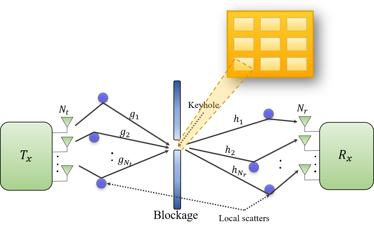
(a)

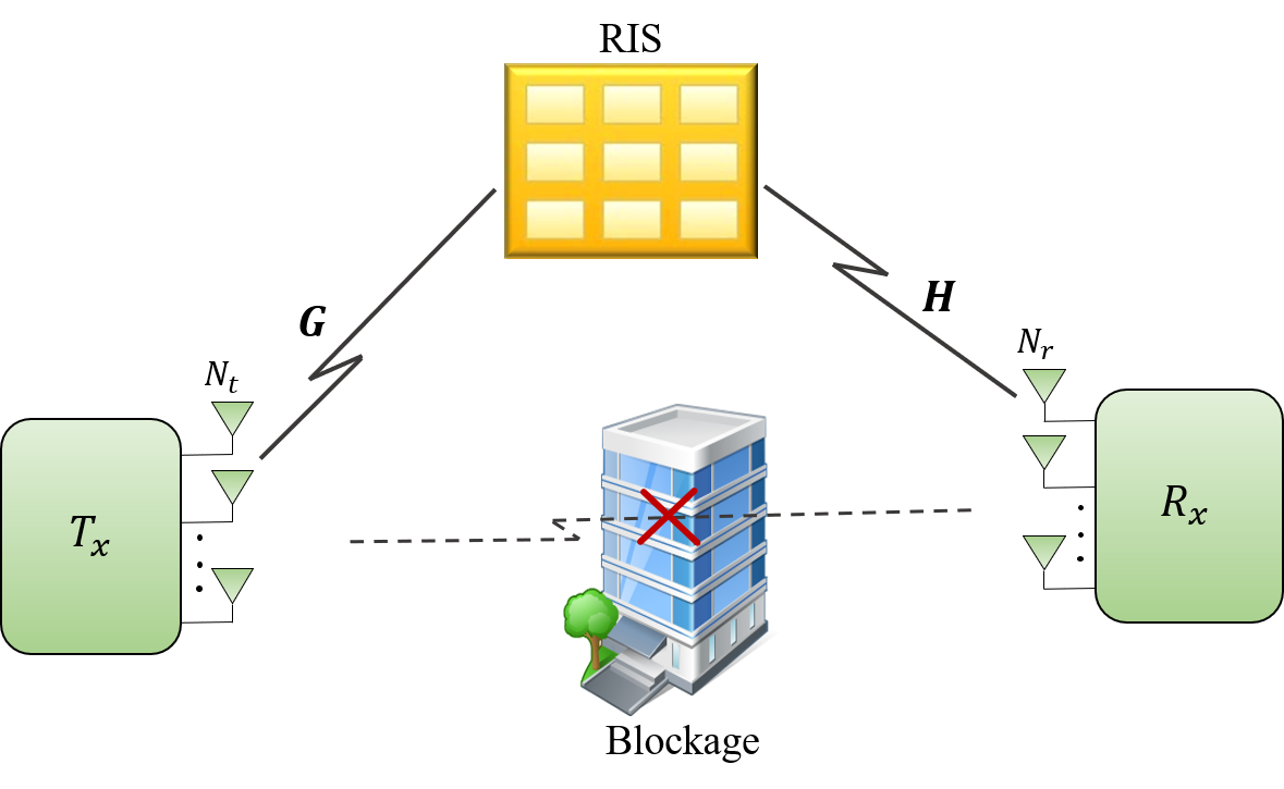
(b)

Figure 1: (a) A single-keyhole MIMO system equivalent to single-element RIS-MIMO system, and (b) RIS-MIMO system model.

In this section, the channel model for RIS is derived based on the concept of keyholes. RIS elements are assumed to be regular scatterers with an ability to control the phases of the scattered signal [1], and the channel model is developed accordingly in this paper. Also, the RIS is assumed to be operating in the far field.

II-A Keyhole MIMO Channel Model

In practice, a MIMO system can also operate in an insufficient scattering environment, which can lead to a rank deficient channel. For example, in a scenario of transmitter and receiver surrounding by clutters (rich scattering environment), where most of the signal energy passes through small holes, the channel rank can reduce to one. This effect has been called ”keyhole”, and the channel is modeled as a keyhole MIMO channel [10]. It can happen when the band of scatterers around the transmitter and the receiver is small compared to the distance between the transmitter and the receiver. Other scenarios for the keyhole effects can be given in [11]. Following similar behaviour, it is proved in [12] that the RIS-MIMO channel model is similar to keyhole MIMO channels by deriving a closed-form approximation to the channel distribution of the RIS-aided systems which is appeared to be equivalent to keyhole channels under some limitations.

The concept of keyhole MIMO channel was firstly introduced in [13], where the channel is considered as a dyad with one degree of freedom which usually appears in a general MIMO relay channel [14]. In a single-keyhole MIMO system model as shown in Fig. 1(a), the total channel matrix can be given as

$$\mathbf{H}_{\mathrm{key}} =\begin{pmatrix}h_{1}\\ \vdots\\ h_{N_{r}}\end{pmatrix}\sigma_{scs}\begin{pmatrix}g_{1}&\cdots&g_{N_{t}}\\ \end{pmatrix},$$ (1)

$$\mathbf{H}_{\mathrm{key}} =\sigma_{scs}\begin{pmatrix}h_{1}g_{1}&\cdots&h_{1}g_{N_{t}}\\ \vdots&\ddots&\vdots\\ h_{N_{r}}g_{1}&\cdots&h_{N_{r}}g_{N_{t}}\end{pmatrix},$$

where $\sigma_{scs}\in[0,1]$ is the scattering cross-section of the keyhole, $g_{1}$ and $g_{2}$ are the complex channel coefficients of the Tx-keyhole channel, $h_{1}$ and $h_{2}$ are the channel coefficients of the keyhole-Rx channel. Clearly, the entries of $\mathbf{H}_{\mathrm{key}}$ are uncorrelated; however, this matrix has only one degree of freedom unlike the case without keyhole (MIMO channel) and hence it has low capacity. Therefore, the SVD of $\mathbf{H_{\mathrm{key}}}$ is written as

$$\mathbf{H}_{\mathrm{key}}=\mathbf{U}\Lambda\mathbf{V}^{H}=\sum_{m=1}^{\min(N_{t},N_{r})}\mathbf{u}_{m}\lambda_{m}\mathbf{v}_{m}^{H}=\mathbf{u}_{1}\lambda_{1}\mathbf{v}_{1}^{H},$$ (2)

where $N_{t}$ and $N_{r}$ are the number of transmit and receive antennas, respectively. This means that the keyhole channel can be represented by only one dyad.

II-B RIS as a Keyhole

From the discussion in Subsection II-A, we can observe that each RIS element is a perfect example of keyhole. This has been expressed in [12], where the authors showed the similarity between their derived RIS-MIMO channel distribution and the keyhole channels distribution.

Considering a MIMO system with $N_{t}$ transmit and $N_{r}$ receive antennas at the Tx and the Rx, respectively. The direct link Tx-Rx is ignored due to the bad propagation conditions. Therefore, an RIS consisting of $N$ elements is deployed to assist the communication. It is assumed that the transmission operates in TDD mode, and local scatterers are randomly distributed quasistatically near the transmit or the received antenna array. Thus, the channel becomes quasistatic, frequency flat, and uncorrelated.

Let $\mathbf{H}^{i}_{T}\in\mathbb{C}^{N_{r}\times N_{t}}$ be the total effective channel between Tx-Rx via the $i$-th RIS element, then given (1), the total channel can be defined as

$$\mathbf{H}_{T}^{i}=\mathbf{h}^{i}\sigma_{scs}^{i}\gamma^{i}e^{j\theta_{i}}\mathbf{g}^{i},$$ (3)

where $\theta_{i}$ is the controlled RIS element phase, $\gamma^{i}$ and $\sigma_{scs}^{i}$ denote the gain and the scattering cross-section of the $i$-th element of the RIS, respectively. $\mathbf{g}^{i}\in\mathbb{C}^{1\times N_{t}}$ and $\mathbf{h}^{i}\in\mathbb{C}^{N_{r}\times 1}$ denote the Tx-$i$-th RIS element and the $i$-th RIS element-Rx channel vectors, respectively. It should be noted that all elements in matrix $\mathbf{H}_{T}^{i}$ are uncorrelated and $\mathbf{h}^{i}$ and $\mathbf{g}^{i}$ are independent, yet, $\mathbf{H}_{T}^{i}$ has a single degree of freedom $\operatorname{rank}(\mathbf{H}_{T}^{i})=1$.

The total Tx-RIS-Rx channel is the sum of the contributions from each RIS element. Therefore, for an RIS-MIMO channel model, the total effective channel is expressed as

$$\mathbf{H}_{T}=\sum_{i=1}^{N}\mathbf{H}_{T}^{i}=\sum_{i=1}^{N}\mathbf{h}^{i}\sigma_{scs}^{i}\gamma^{i}e^{j\theta_{i}}\mathbf{g}^{i}=\mathbf{{H}}\mathbf{\Theta}\mathbf{{G}},$$ (4)

where $\mathbf{H}=[\mathbf{h}^{1},\dots,\mathbf{h}^{N}]$, $\mathbf{{G}}=[(\mathbf{g}^{1})^{T},\dots,(\mathbf{g}^{N})^{T}]^{T}$ and $\mathbf{\Theta}=\operatorname{diag}([\sigma_{scs}^{1}\gamma^{1}e^{j\theta_{1}},\dots,\sigma_{scs}^{N}\gamma^{N}e^{j\theta_{N}}])$ is the diagonal matrix containing the reflection coefficient induced by each element along with its gain and radar cross-section. Throughout this paper, it is considered that $\sigma_{scs}^{i}=\gamma^{i}=1$, for $\forall i$.

III Channel Estimation

To develop the channel estimation algorithm, firstly, the model is derived for only a single RIS element. Then, it is generalized for the whole RIS.

III-A Channel Estimation for Single RIS Element

We consider the $i$-th element of the RIS to be activated, and all other elements to be in the off-mode. The same system model shown in Fig. 1(b) is adopted. The Tx-RIS-Rx channel is given by (3). Using the results concluded in Subsection II-A, the SVD of the single RIS element channel matrix is expressed as

$$\mathbf{H}_{T}^{i}=\mathbf{U}^{i}\Lambda^{i}(\mathbf{V}^{i})^{H}=\mathbf{u}_{1}^{i}\lambda_{1}(\mathbf{v}_{1}^{i})^{H}.$$ (5)

By comparing (5) to (3), it can be seen that $\mathbf{u}_{1}^{i}$ and $(\mathbf{v}_{1}^{i})^{H}$ are normalized and rotated versions of the vectors $\mathbf{h}^{i}$ and $\mathbf{g}^{i}$, respectively, i.e., $\mathbf{h}^{i}=\sqrt{\lambda_{1}}\mathbf{u}_{1}^{i}e^{j\alpha_{i}}$ and $\mathbf{g}^{i}=\sqrt{\lambda_{1}}(\mathbf{v}_{1}^{i})^{H}e^{j\beta_{i}}$, where $e^{\alpha_{i}}$ and $e^{j\beta_{i}}$ ensures that $\mathbf{h}^{i}$ and $\mathbf{g}^{i}$ are not necessarily orthogonal. It is should be noted that $e^{j\alpha_{i}}=e^{-j\beta_{i}}$ therefore, their effect cancels out when multiplied, and estimating channel $\mathbf{H}_{T}^{i}$ is equivalent to estimating $\mathbf{u}_{1}^{i}\lambda_{1}(\mathbf{v}_{1}^{i})^{H}$.

Let $\mathbf{X}=[\mathbf{x}_{1},\dots,\mathbf{x}_{N_{t}}]\in\mathbb{C}^{N_{t}\times N_{t}}$ be the transmitted pilot matrix over the total estimation time slots. It is preferable to design $\mathbf{X}$ and $\mathbf{\Theta}$ to be semi-unitary matrices i.e., $\mathbf{X}\mathbf{X}^{H}=\mathbf{I}$. Then, the received noisy signal ${\mathbf{Y}}\in\mathbb{C}^{N_{r}\times N_{t}}$ is given by

$${\mathbf{Y}}=\widetilde{\mathbf{Y}}+\mathbf{N},$$ (6)

where $\widetilde{\mathbf{Y}}=\mathbf{H}_{T}^{i}\mathbf{X}$ is the received noise-free signal and $\mathbf{N}\in\mathbb{C}^{N_{r}\times N_{t}}$ is the zero-mean AWGN with variance $\sigma^{2}$ .i.e, $\mathbf{N}\sim\mathbb{C}\mathcal{N}(\mathbf{0},\sigma^{2}\mathbf{I})$.

In order to estimate the cascaded channels separately, the proposed algorithm considers two cases as follows

$$\mathbf{Y}\mathbf{Y}^{H} =\mathbf{H}_{T}^{i}\mathbf{X}\mathbf{X}^{H}(\mathbf{H}_{T}^{i})^{H}+\widehat{\mathbf{N}}_{1},$$ (7)

$$=\mathbf{U}^{i}\Lambda^{i}(\mathbf{V}^{i})^{H}\mathbf{X}\mathbf{X}^{H}\mathbf{V}^{i}\Lambda^{i}(\mathbf{U}^{i})^{H}+\widehat{\mathbf{N}}_{1},$$

$$\mathbf{X}\mathbf{Y}^{H} \mathbf{Y}\mathbf{X}^{H}=\mathbf{X}\mathbf{X}^{H}(\mathbf{H}_{T}^{i})^{H}\mathbf{H}_{T}^{i}\mathbf{X}\mathbf{X}^{H}+\widetilde{\mathbf{N}}_{1},$$ (8)

$$=\mathbf{X}\mathbf{X}^{H}\mathbf{V}^{i}\Lambda^{i}(\mathbf{U}^{i})^{H}\mathbf{U}^{i}\Lambda^{i}(\mathbf{V}^{i})^{H}\mathbf{X}\mathbf{X}^{H}+\widehat{\mathbf{N}}_{2},$$

where $\widehat{\mathbf{N}}_{1}$ and $\widehat{\mathbf{N}}_{2}$ are the remaining unwanted part from the equations that include the AWGN. These values are assumed to be small compared to the desired part of the equation, therefore, the rank of the channel matrix remains the same. Since $\mathbf{U}$ is unitary, $(\mathbf{U}^{i})^{H}\mathbf{U}^{i}=\mathbf{I}$, and $\mathbf{X}$ is semi-unitary. Then, by substituting (5) in (7) and (8), we get

$$\mathbf{Y}\mathbf{Y}^{H} =\mathbf{u}_{1}^{i}(\lambda_{1}^{i})^{2}(\mathbf{u}_{1}^{i})^{H}+\widehat{\mathbf{N}}_{1},$$ (9)

$$\mathbf{X}\mathbf{Y}^{H}\mathbf{Y}\mathbf{X}^{H} =\mathbf{v}_{1}^{i}(\lambda_{1}^{i})^{2}(\mathbf{v}_{1}^{i})^{H}+\widehat{\mathbf{N}}_{2}.$$

The result emphasizes that taking the EVD of (9) gives directly $\mathbf{u}_{1}^{i}$, $\mathbf{v}_{1}^{i}$, and $\lambda^{i}_{1}$, and consequently $\mathbf{\tilde{g}}^{i}=(\mathbf{v}_{1}^{i})^{H}$ and $\mathbf{\tilde{h}}^{i}=\lambda_{1}\mathbf{u}_{1}^{i}e^{-j\theta^{i}}$ can be estimated, the term $e^{-j\theta^{i}}$ is added to cancel the phase shift induced by the RIS.

The EVD problem to estimate $\mathbf{\tilde{g}}^{i}$ and $\mathbf{\tilde{h}}^{i}$ is equivalent to the non-iterative least square algorithm in [15] introduced to solve the least square problems $\underset{\mathbf{\tilde{h}}^{i}}{\operatorname{min}}\quad\|\mathbf{Y}\mathbf{Y}^{H}-\mathbf{\tilde{h}}^{i}(\mathbf{\tilde{h}}^{i})^{H}\|^{2}_{F}$ and $\underset{\mathbf{\tilde{g}}^{i}}{\operatorname{min}}\quad\|\left(\mathbf{X}\mathbf{Y}^{H}\mathbf{Y}\mathbf{X}^{H}\right)/(\lambda_{1}^{i})^{2}-(\mathbf{\tilde{g}}^{i})^{H}\mathbf{\tilde{g}}^{i}\|^{2}_{F}$ to get $\mathbf{\tilde{h}}^{i}$, $\lambda_{1}^{i}=\|\mathbf{\tilde{h}}^{i}\|$, and $\mathbf{\tilde{g}}^{i}$, respectively.

III-B Channel Estimation for the Whole RIS

Following the previous subsection, the channel estimation algorithm can be generalized for $N$ RIS elements and can be applied for all RIS-MIMO systems. However, this generalization is not straightforward, and there is a constraint that must be taken into consideration. From (2) and (3), it is found that

$$\mathbf{H}_{T}=\sum_{m=1}^{\min(N_{t},N_{r})}\mathbf{u}_{m}\lambda_{m}\mathbf{v}_{m}^{*}=\sum_{i=1}^{N}\mathbf{h}^{i}\sigma_{scs}^{i}e^{j\theta_{i}}\mathbf{g}^{i}.$$ (10)

This indicates that the EVD channel estimation problem holds only if $\min(N_{t},N_{r})\geq N$. Hence, RIS elements are divided into subgroups $N_{sub}$ with $\min(N_{t},N_{r})$ elements in each subgroup. Thus, the time overhead of the total estimation procedure is $N_{t}\times\lceil\frac{N}{\min(N_{t},N_{r})}\rceil$, where $\lceil\cdot\rceil$ returns the smallest integer value that is bigger than or equal to a number. The subgrouping is recommended to include non-adjacent RIS elements so that the channels estimated are uncorrelated with higher probability. For the $n$-th activated subgroup, the same steps in Subsection III-A can be applied to get

$$\mathbf{Y}^{n}(\mathbf{Y}^{n})^{H}=\mathbf{U}^{n}(\Lambda^{n})^{2}(\mathbf{U}^{n})^{H}+\widehat{\mathbf{N}}_{1}^{n},$$ (11)

$$\mathbf{X}(\mathbf{Y}^{n})^{H}\mathbf{Y}^{n}\mathbf{X}^{H}=\mathbf{V}^{n}(\Lambda^{n})^{2}(\mathbf{V}^{n})^{H}+\widehat{\mathbf{N}}_{2}^{n}.$$ (12)

Since $\min(N_{t},N_{r})$ RIS antenna elements are activated, the estimated channel for the $n$-th subgroup would be full-rank channel, and the channels can be estimated by getting the EVD of both (11) and (12) to get the estimated channels $\mathbf{\tilde{H}}^{n}$ and $\mathbf{\tilde{G}}^{n}$. Therefore, decomposing (11) gives $\Lambda^{n}$ and $\mathbf{U}^{n}$ that are used to find $\mathbf{\tilde{H}}^{n}=\Lambda^{n}\mathbf{U}^{n}(\mathbf{\Theta}^{n})^{-1}$, while decomposing (12) gives $\mathbf{V}^{n}$ which is equal to $\mathbf{\tilde{G}}^{n}$, where $\mathbf{\Theta}^{n}$ is the diagonal matrix containing the phase shifts of the $n$-th RIS subgroup elements.

After $N_{t}\times\lceil\frac{N}{\min(N_{t},N_{r})}\rceil$ time slots, the total estimated MIMO channel of the RIS is given by

$$\mathbf{\tilde{H}}_{T}=\sum_{n=1}^{\lceil\frac{N}{\min(N_{t},N_{r})}\rceil}\mathbf{\tilde{H}}_{T}^{n}=\sum_{n=1}^{\lceil\frac{N}{\min(N_{t},N_{r})}\rceil}\mathbf{\tilde{H}}^{n}\mathbf{\Theta}^{n}\mathbf{\tilde{G}}^{n}.$$ (13)

For further reduction in time overhead of the channel estimation procedure, we enhance the proposed algorithm to compute only one channel and find the other one using the total estimation of the effective channel (i.e., for $N_{t}>N_{r}$ or $N_{t}<N_{r}$ only $\mathbf{\tilde{H}}$ or $\mathbf{\tilde{G}}$ are computed, respectively). For instance, in case of $N_{t}>N_{r}$, $\mathbf{Y}\mathbf{Y}^{H}$ is calculated only, and hence channel $\mathbf{\tilde{H}}^{n}$ is obtained for $n=[1,\dots,\lceil\frac{N}{N_{t}}\rceil]$ subgroups. Next, all RIS are activated and the effective MIMO channel $\mathbf{H}_{T}$ is estimated conventionally by considering the RIS as a random scatterer in the environment [17]. Finally, $\mathbf{\tilde{G}}$ is obtained as

$$\mathbf{\tilde{G}}=\mathbf{\Theta}^{-1}(\mathbf{\tilde{H}}^{H}\mathbf{\tilde{H}})^{-1}\mathbf{\tilde{H}}^{H}\mathbf{\tilde{H}}_{T}.$$ (14)

This would result in further reducing the overhead to $N_{t}\times(\lceil\frac{N}{\max(N_{t},N_{r})}\rceil+1)$. In case $N_{r}>N_{t}$, similar steps can be followed to estimate the cascaded channels. The proposed scheme is summarized in Algorithm 1.

IV Simulation Results

In this section, simulation results are provided to validate the proposed RIS-MIMO model and evaluate the proposed channel estimation framework. The estimation performance is evaluated in terms of normalized mean-square-error (NMSE) and the estimation performance results are obtained by averaging 10000 independent random channel realizations.

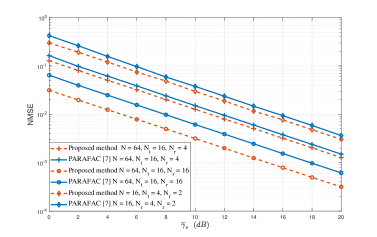
Figure 2: NMSE performance of the effective cascaded channel by proposed channel estimation framework compared to [7].

To evaluate our proposed algorithm, we make a comparison with the first method introduced in [7] namely, LSKRF. For a fair comparison, the same design requirements set in [7] are used to present the performance comparison between the proposed channel estimation framework and the LSKRF method. This comparison is illustrated in Fig. 2 under a different number of transmit/receive antennas and RIS elements. Fig. 2 clearly shows that the proposed method achieves better performance compared to LSKRF [7] in estimating the total effective channel $\mathbf{H}_{T}$. The results indicate that as the number of the receive antenna elements $N_{r}$ increases, the resolution of our proposed method increases, which results in enhancing the estimation performance.

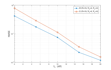
Figure 3: NMSE performance of the cascaded channels separately when $N_{t}=N_{r}=4$ and $N=16$.

In order to show the main advantage of the proposed estimation algorithm, Fig. 3 illustrates the NMSE performance of estimating the cascaded channel separately at $N_{t}=N_{r}=4$ and $N=16$, where the system setup is assumed to be same as in Fig. 2. The performance of each channel link is shown to be similar to conventional MIMO systems with large antenna array size [17], hence, controlling the channel can be feasible for each RIS-MIMO channel link separately, and the type of channel can be identified to enable more functionality such as channel tracking and precoding at the RIS level.

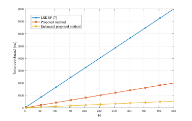
Figure 4: The time overhead of the proposed channel estimation framework compared to [7] for different number of RIS elements when $N_{t}=16$ and $N_{r}=4$.

The time overhead of the proposed channel estimation algorithm with its enhanced version in comparison to LSKRF method [7] is presented in Fig. 4 at different number of RIS elements for $N_{t}=16$ and $N_{r}=4$. It is seen that LSKRF method [7] requires at least $\min(N_{t},N_{r})$ time overhead more than our proposed algorithm for correctly estimating the total channel $\mathbf{H}_{T}$. For example, at $N=256$, the proposed method achieves 75% time overhead reduction compared to LSKRF method [7], while the enhanced version of the proposed algorithm achieves more than 93%. These reduction percentages increase as the number of the RIS elements increases, which results in having more practical and efficient estimation method in terms of both time overhead and estimation performance.

V Conclusion

In this paper, the RIS-MIMO channel is modeled as a keyhole MIMO system. Based on that, we propose two novel channel estimation algorithms by unfolding the RIS-MIMO channel links and then analyzing the components of the cascaded channel applying the EVD separately. The first proposed algorithm provides $\min(N_{r},N_{t})$ times reduction in the system overhead compared to the conventional schemes. The second algorithm is an enhanced version of the first one to further achieve $\max(N_{r},N_{t})$ times reduction in the total estimation duration. As future work, the proposed method can be studied to consider different sparsity levels of the channels Tx-RIS and RIS-Rx.

References

- [1] E. Basar et al., “Wireless communications through reconfigurable intelligent surfaces,” IEEE Access, vol. 7, pp. 116 753–116 773, 2019.
- [2] A. Almohamad et al., “Smart and secure wireless communications via reflecting intelligent surfaces: A short survey,” IEEE Open Journal of the Commun. Society, 2020.
- [3] Z. Wang et al., “Channel estimation for intelligent reflecting surface assisted multiuser communications: Framework, algorithms, and analysis,” IEEE Trans. Wireless Commun., 2020.
- [4] B. Zheng and R. Zhang, “Intelligent reflecting surface-enhanced OFDM: Channel estimation and reflection optimization,” IEEE Wireless Commun. Lett., 2019.
- [5] T. L. Jensen and E. De Carvalho, “An optimal channel estimation scheme for intelligent reflecting surfaces based on a minimum variance unbiased estimator,” in ICASSP 2020-2020 IEEE Int. Conf. Acoust., Speech and Signal Process. (ICASSP), Barcelona, Spain, Spain. IEEE, 2020, pp. 5000–5004.
- [6] L. Wei et al., “Parallel factor decomposition channel estimation in RIS-assisted multi-user MISO communication,” in IEEE 11th SAM Signal Process Workshop. IEEE, 2020, pp. 1–5.
- [7] G. T. de Araújo and A. L. de Almeida, “PARAFAC-based channel estimation for intelligent reflective surface assisted MIMO system,” in IEEE 11th SAM Signal Process Workshop. IEEE, 2020, pp. 1–5.
- [8] S. E. Zegrar et al., “A general framework for RIS-aided mmWave communication networks: Channel estimation and mobile user tracking,” arXiv preprint arXiv:2009.01180, 2020.
- [9] Z.-Q. He and X. Yuan, “Cascaded channel estimation for large intelligent metasurface assisted massive mimo,” IEEE Wireless Communications Letters, vol. 9, no. 2, pp. 210–214, 2019.
- [10] D. Chizhik et al., “Keyholes, correlations, and capacities of multielement transmit and receive antennas,” IEEE Trans. Wireless Commun., vol. 1, no. 2, pp. 361–368, 2002.
- [11] H. Q. Ngo and E. G. Larsson, “No downlink pilots are needed in TDD massive MIMO,” IEEE Trans. Wireless Commun., vol. 16, no. 5, pp. 2921–2935, 2017.
- [12] L. Yang et al., “Accurate closed-form approximations to channel distributions of RIS-aided wireless systems,” IEEE Wireless Commun. Lett., 2020.
- [13] D. Chizhik et al., “Capacities of multi-element transmit and receive antennas: Correlations and keyholes,” Electronics Letters, vol. 36, no. 13, pp. 1099–1100, 2000.
- [14] O. Souihli and T. Ohtsuki, “The MIMO relay channel in the presence of keyhole effects,” in 2010 IEEE Int. Conf. Commun. IEEE, 2010, pp. 1–5.
- [15] A. Y. Kibangou and G. Favier, “Non-iterative solution for PARAFAC with a Toeplitz matrix factor,” in 2009 17th European Signal Processing Conference. IEEE, 2009, pp. 691–695.
- [16] A. F. Molisch, “A generic model for MIMO wireless propagation channels in macro- and microcells,” IEEE Trans. Signal Process., vol. 52, no. 1, pp. 61–71, 2004.
- [17] N. Kim, Y. Lee, and H. Park, “Performance analysis of MIMO system with linear MMSE receiver,” IEEE Transactions on Wireless Communications, vol. 7, no. 11, pp. 4474–4478, 2008.