Pythonic Black-box Electronic Structure Tool (PyBEST). An open-source Python platform for electronic structure calculations at the interface between chemistry and physics

Abstract

Pythonic Black-box Electronic Structure Tool (PyBEST) represents a fully-fledged modern electronic structure software package developed at Nicolaus Copernicus University in Toruń. The package provides an efficient and reliable platform for electronic structure calculations at the interface between chemistry and physics using unique electronic structure methods, analysis tools, and visualization. Examples are the (orbital-optimized) pCCD-based models for ground- and excited-states electronic structure calculations as well as the quantum entanglement analysis framework based on the single-orbital entropy and orbital-pair mutual information. PyBEST is written primarily in the Python3 programming language with additional parts written in C++, which are interfaced using Pybind11, a lightweight header-only library. By construction, PyBEST is easy to use, to code, and to interface with other software packages. Moreover, its modularity allows us to conveniently host additional Python packages and software libraries in future releases to enhance its performance. The electronic structure methods available in PyBEST are tested for the half-filled 1-D model Hamiltonian. The capability of PyBEST to perform large-scale electronic structure calculations is demonstrated for the model vitamin B₁₂ compound. The investigated molecule is composed of 190 electrons and 777 orbitals for which an orbital optimization within pCCD and an orbital entanglement and correlation analysis are performed for the first time.

Institute of Physics, Nicolaus Copernicus University in Toruń] Institute of Physics, Faculty of Physics, Astronomy and Informatics, Nicolaus Copernicus University in Toruń, Grudziadzka 5, 87-100 Torun, Poland Faculty of Chemistry, Nicolaus Copernicus University in Toruń] Faculty of Chemistry, Nicolaus Copernicus University in Toruń, Gagarina 7, 87-100 Torun, Poland Institute of Physics, Nicolaus Copernicus University in Toruń] Institute of Physics, Faculty of Physics, Astronomy and Informatics, Nicolaus Copernicus University in Toruń, Grudziadzka 5, 87-100 Torun, Poland PyBest, AP1roG, PTa, PTb, LCCD, LCCSD, pCCD, EOM-pCCD, EOM-pCCD+S EOM-pCCD-LCCSD, EOM-pCCD-LCCD, SAPT, quantum chemistry software, Python3

1 Introduction

The Pythonic Black-box Electronic Structure Tool (PyBEST) is a modern open-source electronic structure software package developed at Nicolaus Copernicus University (NCU) in Toruń. PyBEST is written primarily in the Python3 programming language (about 90% of the code) with additional parts written in C++ (about 10% of the code, at least C++11 standard), conveniently interfaced using Pybind11, a lightweight header-only library. ¹ The source-code is under the version control (git) and hosted on a gitlab repository server. The PyBEST project started in 2015 (initially under the name of PIERNIK) as a spin-off of the Horton.v2.0.0 software package developed by T. Verstraelen and coworkers ², to which some of us contributed (K.B. and P.T). The newest Horton3 package is split into several modules and covers mainly unique features related to Density Functional Approximations (DFAs), integration algorithms, and molecular dynamics. ³ The PyBEST development team focuses primarily on unconventional wavefunction models based on the pair Coupled-Cluster Doubles (pCCD) ansatz ^{4, 5, 6}, also known as the Antisymmetric Product of 1-reference orbital Geminal (AP1roG) ansatz in the geminal community, and its extensions. Thus, the main driving force for the development of PyBEST is to model large and complex electronic structures that feature both static/non-dynamic and dynamic electron correlation effects using efficient and reliable wavefunction-based methods. On top of that, PyBEST also comprises the standard Coupled-Cluster Singles and Doubles (CCSD) approach and its linearized variants (LCCSD and LCCD), the Möller–Plesset Perturbation Theory of the second-order (MP2) ⁷ and its spin-component scaled variants (SCS-MP2) ⁸, as well as the Symmetry Adapted Perturbation Theory of zeroth-order (SAPT0). ⁹ Over the past few years, PyBEST transformed into a new standalone electronic structure software package that is conveniently applicable at the interface between quantum chemistry and physics. We should stress, however, that the current version of PyBEST uses the original, albeit slightly modified and adjusted Horton v.2.0.0 implementation of SCF acceleration techniques such as the commutator-based direct inversion of the iterative subspace (CDIIS) algorithm ¹⁰, the energy-direct inversion of the iterative subspace (EDIIS) algorithm, the EDIIS2 algorithm (a combination of CDIIS and EDIIS). ¹¹ Since we are exploiting a modified version of the Horton v.2.0.0 SCF code, all complementary modules required to execute an SCF calculation have been adopted as well. These include, among others, the occupation model, orbital instances, and the basic structure of the linear algebra factory and the I/O container. However, neither the SCF implementation of PyBEST nor any other module warrants any backward compatibility with Horton v.2.0.0.

PyBEST’s unique features include the (variational) orbital-optimized pCCD model ^{5, 12}, which allows us to optimize molecular orbitals similar as in the Complete Active Space Self-Consistent-Field ¹³ (CASSCF) procedure but with no restriction on the number of active orbitals or electrons, that is, without the need to define active orbitals spaces. Furthermore, pCCD also provides a cost-effective way to obtain an orbital entanglement and correlation analysis form its response density matrices. ^{14, 15, 16, 17} It opens the way to large-scale modeling and a quantum entanglement analysis of complex electronic structures, which feature a significant amount of strong electron correlation effects. ^{18, 5, 12, 16, 17} The missing part of the dynamic correlation energy in pCCD can be accounted for using either one of the perturbation theory models ^{19, 20, 21} or a (Linearized) Coupled-Cluster ((L)CC) correction. ²² Both the pCCD and pCCD-LCC ansätze have been extended to model excited states using the Equation of Motion (EOM) formalism. ^{23, 24, 25, 26, 27} The first version of the code, PyBEST v1.0.0, was released on July 1, 2020, and is available free of charge. ²⁸ Most recent changes are available at the PyBEST project homepage. ²⁹

2 Program overview

The PyBEST software package comprises the Self-Consistent Field (SCF) module for the Hartree–Fock method, the pCCD module including two different orbital optimization protocols, the Perturbation Theory (PT) module, the CC module, the EOM-CC module, and the SAPT module. These are augmented with post-processing capabilities such as the Pipek–Mezey localization ³⁰, an orbital entanglement and orbital-pair correlation analysis ^{14, 15}, as well as the calculation of the electric dipole and quadrupole moments, where a wrapper is provided for the former. ³¹

2.1 Program capabilities

The PyBEST software package allows us to perform calculations for model Hamiltonians as well as the (non-relativistic) molecular Hamiltonian. Furthermore, it is possible to read in the matrix representation of a Hamiltonian generated by an external software package and perform calculations with PyBEST (e.g., Hartree–Fock, post-Hartree–Fock, and post-processing). Alternatively, the matrix representation of a Hamiltonian (expressed in some molecular orbital basis) can be exported in PyBEST to be imported by external software suits. The communication between different packages is possible through the so-called FCIDUMP ASCII standard present in, for instance, the Molpro ^{32, 33}, Dalton ³⁴, and Budapest DMRG ³⁵ software packages.

2.1.1 The general program structure

The PyBEST software package has a well-defined structure that is similar to all electronic structure methods. Methods implemented in PyBEST operate on and return custom multidimensional array classes that store the actual arrays as their private attributes. Prior to all electronic structure calculations, the user can specify how tensors are represented in PyBEST (see also section 2.1.3). These are, then, combined with a specific Hamiltonian and electronic structure method. The user has full control of the initial conditions and computational workflow by specifying all quantities, e.g., basis set, selected one- and two-electron integrals, occupation model, and initial orbitals (see also sections 2.1.2 and 2.1.4 for more details). Thus, prior to electronic structure calculations with PyBEST, all quantities, like orbitals, occupation models, integrals, etc., need to be defined and initialized.

2.1.2 Hamiltonians and basis sets

In PyBEST v1.0.0, there are two possible choices of Hamiltonians: (i) model Hamiltonians and (ii) the non-relativistic quantum chemical Hamiltonian. Currently as model Hamiltonians, PyBEST supports the 1-dimensional Hubbard Hamiltonian ³⁶ with and without periodic boundary conditions featuring an adjustable hopping and on-site interaction term. The non-relativistic quantum chemical Hamiltonian is constructed from a given molecular geometry and (atom-centered) Gaussian basis sets. The molecular geometry can be either introduced directly using a Python-based input style or read from a .xyz file. The basis set information can be loaded from PyBEST’s basis set library or a user-specified file. Since PyBEST interfaces the basis set reader shipped with Libint (using the modern C++ API), the basis set has to be provided in the .g94 format.

⬇

# create a Gaussian basis set for molecular coordinates provided in mol.xyz

gobasis = get_gobasis("cc-pvdz", "mol.xyz")

PyBEST also allows us to add ghost atoms and mid-bond functions (see section 2.1.11). The complete information about the molecular geometry and basis set (including the molecular orbitals) can be provided directly in PyBEST or read from a file that has been either dumped in PyBEST’s internal .h5 format or generated by some external software in the .molden and .mkl formats. In PyBEST, the molecular Hamiltonian is constructed term-wise, that is, the kinetic energy, the nucleus-electron attraction, and the electron repulsion integrals as well as the nuclear repulsion term. Besides, the overlap integrals of the atom-centered basis set have to be calculated.

⬇

# compute integrals in the atom-centered Gaussian basis set

kin = compute_kinetic(gobasis)

na = compute_nuclear(gobasis)

nuc = compute_nuclear_repulsion(gobasis)

# overlap matrix of the atom-centered Gaussian basis set

olp = compute_overlap(gobasis)

# dense electron repulsion integrals

er = compute_eri(gobasis)

The developer version of PyBEST also supports the (scalar) relativistic Hamiltonians, like the Douglas–Kroll–Hess Hamiltonian of second order. ^{37, 38, 39, 40, 41, 42} Instead of the dense representation of the electron repulsion integrals (ERI), the user can also choose Cholesky-decomposed ERI. ⁴³ The truncation threshold can be changed using the threshold argument (the default value is set to $10^{-3}$).

⬇

# Cholesky-decomposed electron repulsion integrals

er = compute_cholesky_eri(gobasis, threshold=1e-8)

2.1.3 Tensor representations

In version v1.0.0, two tensor representations are available: (i) the dense representation, where all elements (including zeros) are stored, and (ii) Cholesky decomposition, where only the electron repulsion integrals are decomposed, while all smaller dimensional objects are stored in their dense representation. By creating an instance of the selected LinalgFactory class and passing it as an argument during the initialization of quantum chemical methods, the user specifies the preferred tensor representation.

⬇

# create an instance of the dense linalg factory

lf = DenseLinalgFactory(gobasis.nbasis)

# create an instance of the Cholesky linalg factory

lf = CholeskyLinalgFactory(gobasis.nbasis)

The linear algebra module is described in more detail in section 2.2.2.

2.1.4 Molecular orbitals and orbital occupation models

To perform a Hartree–Fock or post-Hartree–Fock calculation, a set of (molecular) orbitals, including their occupation model, has to be defined. In PyBEST, these orbitals contain information on the AO/MO coefficient matrix, the orbital occupation numbers, and the orbital energies.

⬇

# create an empty set of orbitals using the LinalgFactory

orb_a = lf.create_orbital()

In PyBEST, the molecular charge is specified by the number of (singly or doubly) occupied orbitals, that is, the difference between the number of electrons in (singly or doubly occupied) orbitals and the sum of the atomic numbers of all atoms in the molecule. The current version features three different occupation models. In most electronic structure calculations, however, only the AufbauOccModel is supported, where the molecular orbitals are filled with respect to the Aufbau principle.

⬇

# restricted case (six alpha and six beta electrons)

occ_model = AufbauOccModel(6)

# unrestricted case (four alpha and three beta electrons)

occ_model = AufbauOccModel(4, 3)

The fixed occupation model and the so-called Fermi occupation model ⁴⁴ represent alternative choices.

2.1.5 The Hartree–Fock module

To perform an SCF calculation for the Hartree–Fock method, all quantities mentioned above have to be defined, that is, some (molecular) Hamiltonian including the molecular geometry and basis set, a LinalgFactory instance, a set of (molecular) orbitals, and an occupation model. Both the restricted and unrestricted variants of the Hartree–Fock method are implemented. PyBEST offers a convenient wrapper to perform (restricted or unrestricted) Hartree–Fock (RHF and UHF) calculations in an automatic manner. This wrapper combines all terms of the Hamiltonian, generates some initial guess orbitals, chooses a default DIIS solver, and a default convergence threshold. Upon convergence, all Hartree–Fock output data required for restarts and post-processing is returned as an instance of a PyBEST-specific container class.

⬇

# create an instance of the RHF class

hf = RHF(lf, occ_model)

# start an RHF calculation

hf_ = hf(kin, na, er, nuc, olp, orb_a)

A common feature of PyBEST is that the order of the arguments in the function call does not matter as PyBEST exploits internally defined labels for all tensors. Any RHF (or UHF) calculations can be restarted from an internal checkpoint file featuring the .h5 extension. This can be achieved by using the restart keyword and providing the path to the checkpoint file in the function call. By default, all internal checkpoint files are stored in the pybest-results directory using method-specific naming conventions.

⬇

# restart an RHF calculation

hf_ = hf(kin, na, er, nuc, olp, orb_a, restart="pybest-results/checkpoint_scf.h5")

In addition to standard restarts from checkpoint files, PyBEST allows for restarts from perturbed orbitals by swapping orbital pairs or performing manual orbital rotations (Givens rotations), localized orbitals, as well as random unitary rotations of all molecular orbitals. The SCF procedure in PyBEST can be performed with or without acceleration techniques. Possible choices of DIIS solvers include the CDIIS, EDIIS, and EDIIS2 methods ^{10, 11} and can be invoked by the diis keyword. After the SCF algorithm is converged, the final data can be post-processed (e.g., orbital localization) or passed as input to post-HF methods.

2.1.6 The general structure of post-HF modules

All post-HF modules in PyBEST have a similar input structure. To optimize the wavefunction of any post-HF method, the corresponding module requires a Hamiltonian and some orbitals including the overlap matrix (for restart purposes) as input arguments. Note that only the Hamiltonian terms have to be passed explicitly. All remaining information is stored in the HF output container hf_.

⬇

# create an instance of a post-Hartree-Fock method (here called PostHF)

posthf = PostHF(lf, occ_model)

# start the calculation through a function call using the results of

# a previous RHF calculation stored in hf_

posthf_output = posthf(kin, na, er, hf_)

In the above example, PostHF is some post-HF flavor (see below). Thus, the input structure is similar to an HF calculation, except that only all Hamiltonian terms have to be passed explicitly. All post-HF modules support only spin-restricted orbitals and both the DenseLinalgFactory and CholeskyLinalgFactory. Furthermore, PyBEST supports frozen core orbitals, that is, a set of occupied orbitals that is excluded in post-HF calculations as they are assumed to be doubly occupied. This feature is particularly useful when modeling heavier elements for which the core basis functions are generally not optimized for correlated calculations.

2.1.7 The pCCD module

PyBEST supports some unique wavefunction models based on the pCCD ansatz. The pCCD model represents an efficient parameterization of the Doubly Occupied Configuration Interaction (DOCI) wavefunction, ⁴⁵ but requires only mean-field computational cost in contrast to the factorial scaling of traditional DOCI implementations. ^{4, 6} The pCCD wavefunction ansatz can be rewritten in terms of one-particle functions as a fully general pair-Coupled-Cluster wavefunction,

$$|{\rm pCCD}\rangle=\exp\left(\sum_{i=1}^{\rm occ}\sum_{a=1}^{\rm virt}t_{i}^{a}a_{a}^{\dagger}a_{\bar{a}}^{\dagger}a_{\bar{i}}a_{i}\right)|0\rangle=e^{\hat{T}_{\rm p}}|0\rangle,$$ (1)

where $a^{\dagger}_{p}$ and $a_{p}$ ($a^{\dagger}_{\bar{p}}$ and $a_{\bar{p}}$) are the electron creation and annihilation operators for $\alpha$ ($\beta$) electrons, $|0\rangle$ is some reference determinant, $\{t_{i}^{a}\}$ are the electron-pair amplitudes, and $\hat{T}_{\rm p}=\sum_{i=1}^{\rm occ}\sum_{a=1}^{\rm virt}t_{i}^{a}a_{a}^{\dagger}a_{\bar{a}}^{\dagger}a_{\bar{i}}a_{i}$ is the electron-pair excitation operator that excites an electron pair from an occupied $(i\bar{i})$ to a virtual orbital $(a\bar{a})$ with respect to $|0\rangle$. ⁴ PyBEST supports conventional pCCD calculations with a RHF reference function or the orbital-optimized variant (OO-pCCD). ⁵

⬇

# create an instance of RpCCD

pccd = RpCCD(lf, occ_model)

# pCCD calculations

pccd_ = pccd(kin, na, er, hf_)

All results of a pCCD calculation (e.g., electron-pair amplitudes, electronic energies, etc.) are stored as attributes in the pccd$\_$ container.

The pCCD model ensures size-extensivity by construction, requires, however, the optimization of the one-particle basis functions to satisfy size-consistency. PyBEST features two different orbital optimization protocols: (i) variational orbital optimization ⁵ and (ii) the projected-seniority-two orbital optimization in the commutator formulation (PS2c). ¹² By default, the variational orbital optimization protocol is selected.

⬇

# create an instance of ROOpCCD

pccd = ROOpCCD(lf, occ_model)

# (variational) OO-pCCD calculation

pccd_ = pccd(kin, na, er, hf_)

Within the variational orbital optimization scheme, PyBEST performs the calculation of the pCCD response 1- and 2-particle reduced density matrices (1-RDM and 2-RDM), $\gamma^{p}_{q}$ and $\Gamma^{pq}_{rs}$, respectively. Both RDMs are stored as attributes in the pccd$\_$ container. The pCCD 1-RDM is diagonal and is calculated from ^{14, 15}

$$\gamma_{p}^{p}=\langle\Psi_{0}|(1+\hat{\Lambda})a^{\dagger}_{p}a_{p}|\textrm{pCCD}\rangle,$$ (2)

where $\hat{\Lambda}$ contains the de-excitation operator,

$$\hat{\Lambda}=\sum_{ia}\lambda_{i}^{a}(a^{\dagger}_{i}a^{\dagger}_{\bar{i}}a_{\bar{a}}a_{a}-t_{i}^{a}).$$ (3)

The eigenvalues of the response 1-RDM are the pCCD natural occupation numbers. ^{12, 16} The response 2-RDM is defined as

$$\Gamma^{pq}_{rs}=\langle\Psi_{0}|(1+\hat{\Lambda})a^{\dagger}_{p}a^{\dagger}_{q}a_{s}a_{r}|\textrm{pCCD}\rangle.$$ (4)

Since most of the elements of $\Gamma^{pq}_{rs}$ are zero by construction, only the non-zero elements of the response 2-RDM are calculated in PyBEST, which include $\Gamma^{pq}_{pq}=\Gamma^{p\bar{q}}_{p\bar{q}}$ ($\forall\,p\neq q$) and $\Gamma^{p\bar{p}}_{q\bar{q}}$. By default, the orbital optimizer exploits a diagonal approximation to the exact orbital Hessian. The exact orbital Hessian can be calculated separately. However, one should keep in mind that the latter is computationally expensive and hence limited to small and moderate system sizes. To optimize an orbital rotation step, the trust-region or backtracking algorithms can be employed. The former is used by default and combined with Powell’s double-dogleg approximation of the trust region step. ⁴⁶ This particular setup proved to work best for most of the investigated systems. Alternatively, the user can employ the preconditioned conjugate gradient and Powell’s single dogleg step optimization algorithms. ^{47, 48} Orbital optimization within pCCD allows us to obtain qualitatively correct potential energy surfaces and captures a large fraction of strong electron correlation effects. ^{49, 18, 5, 17, 50} Currently, the pCCD module is limited to closed-shell systems only. Various open-shell extensions are currently under development and will be available in future releases of PyBEST.

2.1.8 The CC module

PyBEST supports standard CCD and CCSD as well as their linearized variants, that is, LCCD and LCCSD, on top of a (restricted) Hartree–Fock reference wavefunction. The LCCSD method is equivalent to CEPA(0). All conventional CC calculations can be invoked similarly by creating an instance of the corresponding CC class.

⬇

# create an instance of RCCSD

ccsd = RCCSD(lf, occ_model)

# CCSD calculation

ccsd_ = ccsd(kin, na, er, hf_)

Note that all CC models in PyBEST also support non-canonical orbitals. Thus, the hf$\_$ input container can be substituted by any (converged) reference determinant. In addition to the conventional CEPA(0) approximation, the LCC correction can also be combined with a pCCD reference function (with and without orbital optimization), resulting in the pCCD-LCCD and pCCD-LCCSD approaches. ²² To distinguish between the various linearized CC models, PyBEST v1.0.0 uses a specific class name convention: RHFLCCD, RHFLCCSD, RpCCDLCCD, and RpCCDLCCSD, respectively.

⬇

# create an instance of RpCCDLCCSD

lccd = RpCCDLCCSD(lf, occ_model)

# pCCD-LCCSD calculation with a pCCD reference function

lccd_ = lccd(kin, na, er, pccd_)

Besides, PyBEST allows to perform a standard CC calculations on top of pCCD orbitals. All CC calculations in PyBEST are restartable from .h5 checkpoint files. By default, the krylov solver as implemented in scipy is used. ⁵¹ For all LCC flavors, a Perturbation-based Quasi-Newton (pbqn) solver is also provided. For difficult cases, however, the krylov solver represents a better alternative, despite its slow convergence.

Furthermore, the $\Lambda$ equations for all LCC models can be solved. The corresponding $\lambda$ amplitudes are then used to construct the response RDMs of the LCC wavefunction. In the case of a pCCD reference function, the correlation part can be determined from

$$(\Gamma^{p\ldots}_{t\ldots})^{\rm corr}=\bra{\Phi_{0}}(1+\Lambda^{\prime}) \{e^{-\hat{T}^{\prime}-\hat{T}_{p}}\{\hat{a}^{\dagger}_{p}\ldots a_{t}\}$$

$$e^{\hat{T}_{p}+\hat{T}^{\prime}}\}_{L^{\prime}}\ket{\Phi_{0}},$$ (5)

where $\hat{T}^{\prime}$ ($\Lambda^{\prime}$) contains at most double (de-)excitations, that is $\hat{T}^{\prime}=\hat{T}_{1}+\hat{T}_{2}^{\prime}$ or $\hat{T}^{\prime}=\hat{T}_{2}^{\prime}$ ($\Lambda^{\prime}=\Lambda_{1}+\Lambda_{2}^{\prime}$ or $\Lambda^{\prime}=\Lambda_{2}^{\prime}$), respectively, and

$$\Lambda_{n}^{\prime}=\frac{1}{(n!)^{2}}\sum_{ij\ldots}\sum_{ab\ldots}{}^{\prime}\lambda^{ij\ldots}_{ab\ldots}{i^{\dagger}aj^{\dagger}b\ldots}$$ (6)

is the de-excitation operator, where all electron-pair de-excitation are to be excluded as they do not enter the LCC equations (indicated by the "$\prime$"). Since we work with a linearized coupled-cluster correction, all broken-pair excitation appear at most linear in eq. (2.1.8) (labeled by the subscript $L^{\prime}$). The total $N$-RDM is the sum of the reference contribution, the leading correlation contribution eq. (2.1.8), and all lower-order correlation contributions,

$$\Gamma^{p\ldots}_{t\ldots}=(\Gamma^{p\ldots}_{t\ldots})^{\rm ref}+(\Gamma^{p\ldots}_{t\ldots})^{\rm corr}+\{(\Gamma^{p\ldots}_{t\ldots})^{\rm corr}_{(N-1,\ldots,1)}\},$$ (7)

where the last term indicates all possible lower-order ($N-1,\ldots,1$) correlation contributions to the $N$-RDM in question. For more details see also Ref. 52. The current version of PyBEST automatically calculates (selected elements) of the response 1-, 2-, 3-, and 4-particle RDMs that are required for all supported post-processing schemes (see section 2.1.12) when the $\Lambda$ equations are to be solved. This can be invoked by setting the keyword argument l=True.

⬇

# creat an instance of pCCD-LCCSD

lccsd = RpCCDLCCSD(lf, occ_model)

# also solve the corresponding Lambda equations

lccsd_ = lccsd(kin, na, er, pccd_, l=True)

The developer version of PyBEST also features tailored coupled cluster methods, like the frozen-pair CCSD flavours. ^{53, 54}

2.1.9 The EOM-CC module

The released version of PyBEST allows us to calculate electronically excited states using the EOM-pCCD and EOM-pCCD+S approaches. ^{23, 24}

⬇

# create an instance of REOMpCCD

eom = REOMpCCD(lf, occ_model)

# calculate 3 lowest-lying roots

eom_ = eom(kin, na, er, pccd_, nroot=3)

The EOM-pCCD ansatz includes only the electron-pair excitations in the EOM ansatz while the EOM-pCCD+S flavor comprises both singles and electron-pair excitations. The developer version of PyBEST also supports the EOM-pCCD-LCCD and EOM-pCCD-LCCSD variants. More details about those methods are available in Ref. 25.

2.1.10 The perturbation theory module

PyBEST features perturbation theory-based calculations on top of a (canonical) restricted Hartree–Fock and a pCCD reference function. For the former, PyBEST offers the conventional Møller–Plesset perturbation theory model of second order.

⬇

# create an instance of the RMP2 class

mp2 = RMP2(lf, occ_model)

# perform conventional MP2 calculation on RHF canonical orbitals

mp2_ = mp2(kin, na, er, hf_)

The MP2 module also supports the calculation of (relaxed and unrelaxed) 1-particle reduced density matrices (1-RDM) and the corresponding natural orbitals. Besides the conventional MP2 implementation, the Spin-Component-Scaled (SCS) variant is also implemented including the corresponding (relaxed and unrelaxed) 1-RDM. The same-spin and opposite-spin scaling factors are defined using the keyword arguments fss and fos in the function call. Furthermore, the contributions of single excitations can be accounted for through the singles keyword argument.

⬇

# restricted MP2 calculation with single and double excitations

mp2_ = mp2(kin, na, er, hf_, singles=True)

While single excitations have no effect on the MP2 energy calculated on top of the canonical Hartree–Fock reference, this is no longer the case for non-canonical orbitals like pCCD-optimized orbitals.

Finally, PyBEST provides various unique perturbation theory models with a pCCD reference function that goes beyond the MP2 standard. ¹⁹ Specifically, these perturbation theory corrections offer different choices for the zeroth-order Hamiltonian, perturbation, dual space, and projection manifold. All possible combinations of these degrees of freedom lead to the development of the so-called PT2X models. Possible choices for PT2X are: (i) PT2SDd (single determinant dual state and diagonal one-electron zero-order Hamiltonian), (ii) PT2MDd (multi determinant dual state and diagonal one-electron zero-order Hamiltonian), (iii) PT2SDo (single determinant dual state and off-diagonal one-electron zero-order Hamiltonian), (iv) PT2MDo (multi determinant dual state and off-diagonal one-electron zero-order Hamiltonian), and (v) PT2b. ^{20, 19} By default, the projection manifold is restricted to double excitations but single excitations can be accounted for as well (again using the singles keyword argument).

⬇

# create an instance of the PT2MDo class

pt2 = PT2MDo(lf, occ_model)

# perform PT2MDo calculations including single and double excitations

pt2_ = pt2(kin, na, er, pccd_, singles=True)

The other perturbation theory corrections can be invoked by creating instances of the perturbation theory classes (i) to (v).

2.1.11 Fragment-based calculations

PyBEST provides a flexible interface to handle atomic basis sets such that dummy or ghost atoms and active molecular fragments can be easily defined. Specifically, all dummy/ghost atoms, as well as active fragments have to be passed to the basis set reader function. Both ghost/dummy atoms and active fragments can be used as either joint or separate arguments. To specify the former, the dummy argument has to be used, where all dummy/ghost atoms are indicated as a list containing the indices of all atoms in question. The atoms are indexed with respect to their order in the .xyz file (Python indexing convention).

⬇

# set first (0) and second (1) element as dummy/ghost atom

gobasis = get_gobasis("cc-pvdz", "mol.xyz", dummy=[0,1])

Active fragments are defined in a similar manner.

⬇

# molecule containing atoms 3, 4, and 5 as active fragment

gobasis = get_gobasis("cc-pvdz", "mol.xyz", active_fragment=[3,4,5])

The inactive fragment will be neglected during the construction of the basis set and molecular Hamiltonian. Such fragment-based calculations are particularly useful in the SAPT module, where the molecular Hamiltonian is partitioned into (presumably) weakly interacting fragments ^{55, 56}

$$H=H_{\textrm{A}}+H_{\textrm{B}}+V.$$ (8)

The first two terms in the above equation correspond to the Hamiltonians of the monomers A and B, respectively, and $V$ is the interaction between them. Such a partitioning defines the perturbation series in powers of $V$ with a $\Psi_{\rm A}\Psi_{\rm B}$ zeroth-order wavefunction. PyBEST’s SAPT module currently supports the so-called SAPT0 approximation which neglects the effects of the intramonomer correlation energy on the interaction energy components. In other words, the zeroth-order wavefunction is a product of Slater determinants. ⁹

⬇

# create an instance of SAPT0

sapt0 = SAPT0(monA, monB)

# SAPT0 calculations

sapt0(monA, monB, dimer)

PyBEST is shipped with a utility function sapt_utils.prepare_cp_hf that automatically calculates all necessary ingredients for SAPT0 calculations containing the fragments monA and monB as well as the supermolecule dimer. Furthermore, this wrapper allows us to perform the dimer centered basis set (DCBS) counter-poised corrected Restricted Hartree–Fock calculations in an automatic manner. Each correction to the SAPT0 interaction energy has a physical meaning (see Refs. 55, 56 for more details) and can be accessed term-wise through a dictionary.

⬇

# SAPT0 dictionary

corrections = sapt0_solver.result

# term-wise contributions to the interaction energy

e10_elst = corrections["E^{(10)}_{elst}"]

e10_exch = corrections["E^{(10)}_{exch}(S^2)"]

e20_ind = corrections["E^{(20)}_{ind},unc"]

e20_exch_ind = corrections["E^{(20)}_{exch-ind}(S^2),unc"]

e20_disp = corrections["E^{(20)}_{disp},unc"]

e20_exch_disp = corrections["E^{(20)}_{exch-disp}(S^2),unc"]

All implemented expressions are based on the molecular orbital formulation with the $S^{2}$ approximation for the exchange terms.

2.1.12 Post-processing: orbital-based analysis and visualization

The released version of PyBEST supports various post-processing options of electronic wavefunctions and Hamiltonians. These include dumping orbitals and Hamiltonians to disk using various file formats, (Pipek-Mezey) localization, the calculation of electric dipole moments, and an orbital-based entanglement and correlation analysis. To visualize molecular orbital, they can be dump to disk within the .molden format and then visualized using some orbital visualization program. PyBEST interfaces libint’s export molden feature. In order to dump molecular orbitals to a .molden file, the to_file method implemented in the IOData container can be used.

⬇

# dump pCCD orbitals stored in the pccd_ container

# update container to contain the atomic basis set

pccd_.gobasis = gobasis

# write molden file

pccd_.to_file("my_pccd_orbitals.molden")

Note that the pccd_ container has to be updated to include the basis set information explicitly.

Orbital entanglement and correlation represent a unique feature of PyBEST and allow us to dissect various wavefunction models using the picture of interacting orbitals. ^{57, 58, 14, 15} This allows us to quantify the interaction between orbitals and to understand chemical processes. The interaction between orbitals can be determined using concepts of quantum information theory. Specifically, to measure the entanglement between one orbital and remaining sets of orbitals, PyBEST uses the single-orbital entropy $\rm{s(1)_{i}}$, defined as follows

$$s(1)_{i}=-\sum_{\alpha=1}^{4}\omega_{\alpha;i}\ln(\omega_{\alpha;i}),$$ (9)

where $\omega_{\alpha;i}$ are the eigenvalues of the one-orbital reduced density matrix (1-ORDM). Analogously, the two-orbital entropy $\rm{s_{i,j}}$ is constructed as

$$s_{i,j}=-\sum_{\alpha=1}^{16}\omega_{\alpha;i,j}\ln(\omega_{\alpha;i,j}),$$ (10)

and quantifies the interaction of an orbital pair $i$,$j$, and all other orbitals. The $\omega_{\alpha;i,j}$ are the eigenvalues of the two-orbital RDM with all possible variants of states for spatial orbitals. The above quantities are exploited to calculate the orbital-pair mutual information,

$$I_{i|j}=s_{i}+s_{j}-s_{i,j},$$ (11)

which determines the correlation between the orbital pair $i$ and $j$ embedded in the environment of all other orbitals. The matrix elements of the 1- and 2-ORDMs can be expressed in terms of the $N$-particle RDMs (see, for instance, Refs. 14 and 15). The orbital-pair mutual information allows us to dissect electron correlation effects into different contributions and (together with the single-orbital entropy) represents a useful tool to define optimal and balanced active spaces. ^{59, 14, 60, 61, 62, 63, 64, 65}

The released version of PyBEST supports an orbital entanglement and correlation analysis for the pCCD and LCC wavefunction models.

⬇

# orbital entanglement module

# pCCD

entanglement = OrbitalEntanglementRpCCD(lf, pccd_)

entanglement()

# pCCD-LCCSD

entanglement = OrbitalEntanglementRpCCDLCC(lf, lccsd_)

entanglement()

The entanglement module dumps all output data to separate files containing the single-orbital entropy, orbital-pair mutual information, and the eigenvalue spectra (including the eigenvectors) of the 1- and 2-ORDMs. PyBEST is shipped with a script pybest-entanglement.py that allow us to visualize the single-orbital entropy and orbital-pair mutual information in separate graphs (see appendix B for examples).

2.2 Implementation details

2.2.1 The Libchol library

PyBEST is shipped with a standalone C++ library libchol that provides the routines to generate Cholesky decomposed electron repulsion integrals (ERIs) ⁴³. Specifically, libchol is partially optimized and constitutes a parallelized part of the PyBEST software package. It, however, represents an optional library, and hence all modules implemented in PyBEST run without it. As PyBEST, the libchol library uses the modern C++ API of Libint ⁶⁶ in order to generate blocks of the exact four-center ERIs exploiting MKL’s basic linear algebra subprograms BLAS-2 and BLAS-3 for the decomposition algorithm. ⁶⁷ While the libchol library is at an early stage of its development, it provides already a core functionality for the decomposition of ERIs of the orbital basis,

$$(\mu\nu|\rho\sigma)\approx(\mu\nu|P)(P|\rho\sigma),$$ (12)

where $P$ is the ad-hoc generated Cholesky auxiliary basis set. The current implementation of libchol works exclusively in the in-core memory scheme, and thus is limited to medium-size systems with up to, let’s say, 1000 basis functions depending on the chosen decomposition threshold. Future work includes the out-of-core algorithm and further optimizations allowing us to reduce the required in-core memory and bandwidth.

2.2.2 The Linear Algebra Factory (LinalgFactory) and the tensor contraction engine

The linalg module contains two types of tensor representations: dense tensors and Cholesky-decomposed ERIs, which represent a special type of 4-index objects in PyBEST. All lower-dimensional tensors are always represented as dense numpy arrays.

⬇

# dense electron repulsion integrals

dense_er = compute_eri(gobasis)

# cholesky-decomposed electron repulsion integrals

cholesky_er = compute_cholesky_eri(gobasis, threshold=1e-8)

# create two-dimensional array filled with random numbers

operand = DenseTwoIndex(gobasis.nbasis)

operand.randomize()

Algebraic operations, like addition, tensor contraction, and slicing, are implemented as methods. Specifically, PyBEST’s tensor contraction and slicing are abstract layers that provide a standardized interface to various implementations of tensor contraction operations. They are independent of the internal representation of the many-index objects. Thus, the syntax for DenseFourIndex and CholeskyFourIndex classes is the same even if their internal representation is different as a CholeskyFourIndex class stores three-index arrays.

⬇

# The following four lines provide the same result (within the accuracy of the Cholesky Decomposition)

A = dense_er.contract("abcd,ab", operand)

B = cholesky_er.contract("abcd,ab", operand)

C = operand.contract("ab,abcd", dense_er)

D = operand.contract("ab,abcd", cholesky_er)

Since there are many options to perform these kind of algebraic operations (both in Python and PyBEST), the contract method offers a unified interface for opt_einsum.contract,⁶⁸ numpy.tensordot, numpy.einsum,^{69, 70} and PyBEST’s BLAS-optimized operations. The latter ones are implemented for some bottleneck operations that are complementary to the automatic procedures of the external libraries.

⬇

# example of application of different tensor contraction engines

# opt_einsum.contract

E = cholesky_er.contract("abcd,cb->ad", operand, select="opt_einsum")

# numpy.tensordot

F = cholesky_er.contract("abcd,cb->ad", operand, select="td")

# numpy.einsum

G = cholesky_er.contract("abcd,cb->ad", operand, select="einsum")

# BLAS-optimized operation

H = cholesky_er.contract("abcd,cb->ad", operand, select="blas")

PyBEST is also shipped with different python-based algorithms to perform a 4-index transformation. It further provides a convenient wrapper transform_integrals that automatically transforms all one- and two-electron integrals into the molecular orbital basis. This transformation can be performed either for restricted or unrestricted orbitals. Note that the order of the arguments does not matter.

⬇

# perform an AO/MO transformation of all one- and two-electron integrals

# restricted orbitals

ti = transform_integrals(kin, na, er, orb_a)

# equivalent to

ti = transform_integrals(orb_a, kin, er, na)

# unrestricted orbitals (alpha, beta)

ti = transform_integrals(kin, na, er, orb_a, orb_b)

By default, PyBEST exploits numpy.tensordot to perform the AO/MO transformation. Other options ("tensordot" or "einsum") are also possible and are steered using the indextrans keyword argument. For both flavors, PyBEST successively transforms each index. For the option "tensordot", the lower-level routine looks as follows, where the transformed integrals are stored in-place,

⬇

# PyBEST’s lower-level routine to perform a 4-index transformation

# due to the way tensordot works, the order of the dot products is

# not according to literature conventions

# for restricted orbitals, we have orb0=orb1=orb2=orb3

self._array[:] = np.tensordot(

ao_integrals._array, orb0.coeffs, axes=([0], [0])

)

self._array[:] = np.tensordot(

self._array, orb1.coeffs, axes=([0], [0])

)

self._array[:] = np.tensordot(

self._array, orb2.coeffs, axes=([0], [0])

)

self._array[:] = np.tensordot(

self._array, orb3.coeffs, axes=([0], [0])

)

2.3 Code documentation and distribution

The documentation of PyBEST is generated from sources in the reStructuredText format using Sphinx ⁷¹ and shipped with the code. ²⁸ The most recent documentation is also available on the PyBEST homepage. ²⁹ The documentation covers basic information about the program, license information, how to install it on different operating systems (including dependencies), and a detailed user manual with numerous illustrative examples of how to use the code and its unique features. Furthermore, to improve the understanding of larger parts of the code, such as classes, modules, and functions, we use Python Docstrings. This practice greatly improves code readability and facilitates familiarizing new developers with the code. Similar to the source code, the documentation is under version control (Git) and hosted on a GitLab repository server.

The PyBEST software package is distributed in the source code form under an open-source GNUv3 (General Public License) license. The source code can be easily downloaded from the Zenodo platform ⁷², where the software package has been minted a permanent DOI number, and its metrics are available. A future PyBEST release will be assigned to a different DOI number and shipped with a version-specific documentation. Additional information is available on the PyBEST project homepage. ²⁹

3 Example calculations using PyBEST

3.1 Electronic structure calculations on the 1-D Hubbard Hamiltonian

The 1-D Hubbard Hamiltonian represents a useful model for assessing the accuracy and reliability of newly developed electronic structure methods. ^{73, 5, 6, 17} Modifying the repulsive on-site interaction parameter ${U}$ allows us to control the strength and nature of electron correlation, where strong correlation dominates for larger $U/t$ values. Table 1 summarizes the performance of various quantum chemistry models available in PyBEST in predicting the total and correlation energies for selected values of $U/t$. We focus on the half-filled 1-D Hubbard Hamiltonian with 50 sites and periodic boundary conditions, for which the exact results can be determined by solving the Lieb-Wu equations. ⁷⁴ An example PyBEST input file is shown in Appendix A. Specifically, we investigate three $U/t$ values, namely $U/t=1$, $U/t=2$, and $U/t=3$. This mimics the (strong) electron correlation regime usually encountered in molecular systems. It is evident from Table 1 that the OO-pCCD method combined with one of the dynamic energy corrections provides reliable energies, even for cases where the CCSD method fails to converge. For a detailed discussion on the performance of various OO-pCCD-LCC approaches for the 1-D Hubbard model, we refer the reader to Ref. 52.

Table 1: Performance of various wavefunction models available in PyBEST for the half-filled 1-D Hubbard model Hamiltonian for 50 sites with periodic boundary conditions and different values of the repulsive on-site interaction parameter ${U}$ [$U/t$].

Method	Total energy $[E_{h}]$			Correlation energy $[E_{h}]^{\dagger}$
	$U/t=1$	$U/t=2$	$U/t=3$	$U/t=1$	$U/t=2$	$U/t=3$
RHF	$-$51.203 884	$-$38.703 884	$-$26.203 884	-	-	-
MP2(RHF)⋆	$-$52.051 806	$-$42.095 570	$-$33.835 177	$-$0.847 922	$-$3.391 686	$-$7.631 293
MP2(OO-pCCD)∙	$-$52.001 992	$-$41.818 037	$-$33.552 933	$-$0.798 108	$-$3.114 153	$-$7.349 049
pCCD	$-$51.254 320	$-$38.875 387	$-$26.542 450	$-$0.050 435	$-$0.171 503	$-$0.338 566
OO-pCCD	$-$51.789 439	$-$41.256 975	$-$32.564 839	$-$0.609 173	$-$2.553 095	$-$6.360 955
OO-pCCD-PT2SDd	$-$51.974 875	$-$41.790 323	$-$33.632 419	$-$0.770 991	$-$3.086 443	$-$7.428 535
OO-pCCD-PT2SDo	$-$52.021 235	$-$41.763 875	$-$33.072 400	$-$0.817 351	$-$3.059 991	$-$6.868 516
OO-pCCD-PT2MDd	$-$51.996 174	$-$41.956 922	$-$34.169 938	$-$0.792 290	$-$3.253 038	$-$7.966 054
OO-pCCD-PT2MDo	$-$52.022 636	$-$41.813 367	$-$33.449 709	$-$0.818 752	$-$3.109 483	$-$7.245 825
OO-pCCD-PT2b	$-$52.032 318	$-$42.007 466	$-$34.077 901	$-$0.828 434	$-$3.303 582	$-$7.874 017
OO-pCCD-LCCD	$-$51.994 451	$-$41.745 555	$-$33.195 425	$-$0.790 567	$-$3.041 671	$-$6.991 541
OO-pCCD-LCCSD	$-$52.047 516	$-$42.262 870	$-$34.225 963	$-$0.843 632	$-$3.558 986	$-$8.022 079
CCSD(RHF)⋆	$-$52.054 930	$-$42.156 172	∗	$-$0.851 046	$-$3.452 288	∗
CCSD(OO-pCCD)∙	$-$52.054 855	$-$42.164 166	∗	$-$0.850 971	$-$3.460 282	∗
Exact‡	$-$52.059 828	$-$42.244 338	$-$34.517 041	$-$0.855 944	$-$3.540 454	$-$8.313 157

• ^† Calculated w.r.t RHF.
  

• ^‡ Calculated by solving the Lieb–Wu equations.
  

• ^⋆ Calculated with an RHF reference function.
  

• ^∙ Calculated with an OO-pCCD reference function (OO-pCCD orbitals).
  

• ^∗ Not converged.
  

3.2 Electronic structure, orbital entanglement, and electron correlation effects in the model vitamin B_12 compound

Cobalamins represent a unique group of cobalt-containing complexes that function as cofactors for various enzymes like mutases and transferases. ⁷⁵ The reactivity of the organometallic Co–C bond, which is broken during catalysis, is an active field of research in bioinorganic chemistry. The complex electronic structure and unusually strong multi-reference character of cobalamins attracted a lot of attention from the quantum chemistry community in recent years. ^{76, 77, 78, 79, 80, 81, 82} However, the large size of cobalamin complexes prohibits the application of highly-accurate wavefunction-based quantum chemistry methods and led to the development of cobalt(I)corrin model compounds. A simplified, but still realistic model complex is composed of the cobalt atom and a corrin ring (see Figure 1). This simplified cobalamin-derived compound proved to be an extremely valuable model system in the computational biochemistry community. ^{77, 82} The computational challenge with this model compound comes from its complex, yet not fully understood, electronic structure. A CASSCF/CASPT2 study by Jensen ⁷⁷ shows that the ground state electronic structure of cob(I)alamin is composed of a closed-shell Co(I) d⁸ electron configuration (67%) and a diradical Co(II)d⁷-radical corrin $\pi^{*1}$ electron configuration (23%). Yet, the composition of the active space for the cob(I)alamin compound, comprising only 10 electrons distributed in 11 orbitals, CAS(10,11), remains an open question. ⁷⁷

This motivated us to study the electronic structure of the model vitamin B_12 with the OO-pCCD method available in PyBEST. We used the B3LYP optimized structure from Ref. 79 and Dunning’s aug-cc-pvdz basis set ⁸³, which results in a system comprising 190 electrons and 777 orbitals. Specifically, in our OO-pCCD calculations, we utilized Cholesky-decomposed electron repulsion integrals (determined with libchol) with a threshold value of 1e-6 and a frozen core containing the 32 lowest-lying orbitals. These frozen-core orbitals were optimized by the RHF method. Thus, our active orbital space comprises 126 electrons distributed in 745 orbitals. Our results are summarized in Figure 2 displaying the orbital-pair mutual information of selected orbitals (nos. 60–129) on the left panel and the decay of the orbital-pair mutual information on the right panel. Specifically, the strength of the mutual information is color-coded in descending order, black ($I_{i|j}$> 1.0), blue ($I_{i|j}$> 0.1), red ($I_{i|j}$> 0.001), and green ($I_{i|j}$> 0.001). It is evident from Figure 2(a) that the largest correlations are between the d${}_{z^{2}}$+$\pi$-type bonding orbital and its d${}_{z^{2}}$+$\pi^{*}$-type anti-bonding counterpart, and between the $\pi$-type and $\pi^{*}$-type orbitals of the corrin ring. Non-negligible contributions also arise from the $\sigma$-type and $\sigma^{*}$-type orbitals of the corrin ring. That means that all of them (70 in total) should be considered as important in the composition of an active orbital space (in the pCCD optimized basis). This is also confirmed by a jump in the decay of $I_{i|j}$ in Figure 2(b).

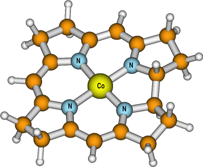
Figure 1: The chemical model of the vitamin B₁₂ complex that includes the corrin ring.

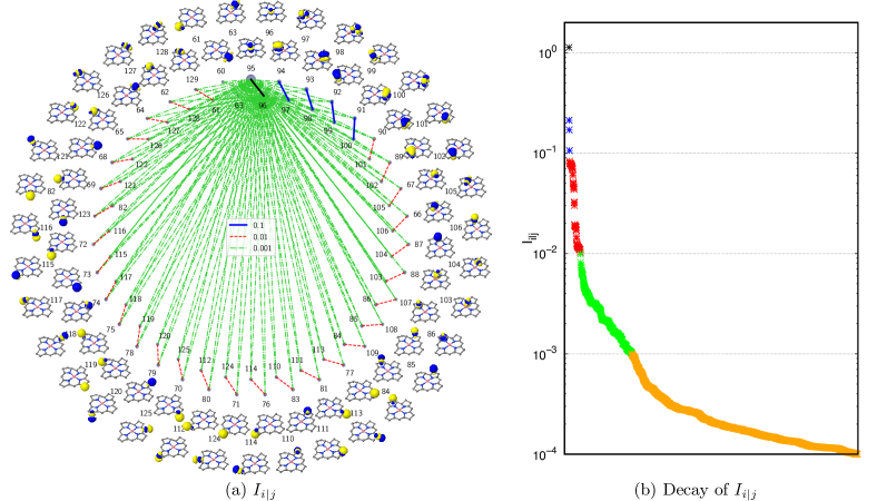
Figure 2: Orbital-pair correlation diagrams for the vitamin B₁₂ model complex. (a) Orbital-pair mutual information for orbitals nos. 60 to 129. The corresponding isosurface plots are shown in the outermost circle. (b) Decay of the orbital-pair mutual information for $I_{i|j}\geq 10^{-4}$. In total, there are more than 277’000 nonzero orbital-pair correlations. The orbitals were visualized using the Jmol software package. ⁸⁴

4 Conclusions and outlook

We have presented the PyBEST software package — a modern open-source electronic structure platform for ab inito calculations at the interface between chemistry and physics. One of the strengths of the code is its unique functionality and modern design based on the Python3 and C++ programming languages interfaced with the Pybind11 header-only library. In addition to standard quantum chemistry methods, PyBEST hosts one-of-a-kind electronic structure approaches based on the pCCD model and its extensions, as well as a quantum entanglement and electron correlation analysis. PyBEST functionality is demonstrated for the 1-D Hubbard model Hamiltonian and the vitamin B_12 model system with an active space composed of 126 electrons distributed in 745 orbitals.

PyBEST is designed to host additional software libraries and serves as a hub for future modular software development efforts. Specifically, the flexible design of the tensor contraction engine in PyBEST, described in section 2.2, enables us to conveniently improve bottleneck operations by, for instance, including additional Python or numpy features, interfacing external libraries like einsum2, ⁸⁵ or optimizing PyBEST’s internal BLAS routines without the need of changing any wavefunction modules profoundly. Moreover, PyBEST allows us to exploit the internal parallelization of BLAS and numpy.tensordot (if numpy is linked to a parallel implementation of BLAS). Further improvements are possible with the aid of Graphical Processor Units (GPUs) and the cupy array library accelerated by CUDA. ⁸⁶ Besides the technical aspects of code optimization, PyBEST also offers an excellent opportunity for the development of novel electronic structure methods. Each of the implemented wavefunction modules can be easily extended with additional methods. A combination of different modules is also possible. The latter is particularly useful for the development of the SAPT module, where symmetry adapted perturbation theory can be uniquely combined with pCCD-based methods, as well as for the design and development of embedding-based methods. ⁸⁷ All these features make PyBEST an exceptional and flexible programming platform for the quick implementation of unique electronic structure methods, followed by large-scale modelling of electronic structures, their visualization and analysis. Finally, PyBEST is under continuous development and version control (using git on Gitlab), where up to date patches containing bug fixes and improvements are available on the PyBEST homepage. ²⁹

Appendix A Example input file for the Hubbard model Hamiltonian

⬇

from pybest import *

# define LinalgFactory for 50 sites

lf = DenseLinalgFactory(50)

# define Occupation model and expansion coefficients

occ_model = AufbauOccModel(25)

orb = lf.create_orbital(50)

# initialize Hubbard class

modelham = Hubbard(lf, pbc=True)

# one and two-body interaction terms defined for the on-site basis

# t-param, t = -1

hopping = modelham.compute_one_body(-1)

# U-param, U = 1

onsite = modelham.compute_two_body(1)

# overlap matrix for on-site basis

olp = modelham.compute_overlap()

# do a Hartree-Fock calculation

hf = RHF(lf, occ_model)

hf_ = hf(hopping, onsite, olp, orb)

# do MP2 optimization

mp2 = RMP2(lf, occ_model)

mp2_ = mp2(hopping, onsite, hf_)

# do CCSD optimization

ccsd = RCCSD(lf, occ_model)

ccsd_ = ccsd(hopping, onsite, hf_)

# do OO-pCCD optimization

oopccd = ROOpCCD(lf, occ_model)

oopccd_ = oopccd(hopping, onsite, hf_)

# run until convergence

while(not oopccd_.converged):

oopccd = ROOpCCD(lf, occ_model)

oopccd_ = oopccd(hopping, onsite, oopccd_)

# do MP2 optimization with pCCD reference

mp2 = RMP2(lf, occ_model)

mp2_ = mp2(hopping, onsite, oopccd_)

# do CCSD optimization with pCCD reference

ccsd = RCCSD(lf, occ_model)

ccsd_ = ccsd(hopping, onsite, oopccd_)

# do PT2 corrections

pt2 = PT2SDd(lf, occ_model)

pt2_ = pt2(hopping, onsite, oopccd_)

pt2 = PT2SDo(lf, occ_model)

pt2_ = pt2(hopping, onsite, oopccd_)

pt2 = PT2MDd(lf, occ_model)

pt2_ = pt2(hopping, onsite, oopccd_)

pt2 = PT2MDo(lf, occ_model)

pt2_ = pt2(hopping, onsite, oopccd_)

pt2 = PT2b(lf, occ_model)

pt2_ = pt2(hopping, onsite, oopccd_)

# do RpCCD-LCCD calculation

lccd = RpCCDLCCD(lf, occ_model)

lccd_ = lccd(hopping, onsite, oopccd_)

# do RpCCD-LCCSD calculation

lccd = RpCCDLCCSD(lf, occ_model)

lccd_ = lccd(hopping, onsite, oopccd_)

Appendix B Example input file for Vit B12

⬇

from pybest import *

# set up molecule, define basis set

occ_model = AufbauOccModel(95)

obasis = get_gobasis("aug-cc-pvdz", "coiicor.xyz")

lf = CholeskyLinalgFactory(obasis.nbasis)

orb = lf.create_orbital(obasis.nbasis)

olp = compute_overlap(obasis)

# construct Hamiltonian

kin = compute_kinetic(obasis)

ne = compute_nuclear(obasis)

er = compute_cholesky_eri(obasis, threshold=1e-6)

external = compute_nuclear_repulsion(obasis)

# restricted Hartree-Fock calculation

scf = RHF(lf, occ_model)

hf = scf(kin, ne, er, external, olp, orb)

# orbital-optimized pCCD calculation

pccd = ROOpCCD(lf, occ_model, ncore=32)

pccd_ = pccd(kin, ne, er, hf)

# execute until convergence

while(not pccd_.converged):

pccd = ROOpCCD(lf, occ_model, ncore=32)

pccd_ = pccd(kin, ne, er, pccd_)

# Dump molden file of current solution

pccd_.gobasis = obasis

pccd_.to_file("pybest-results/pccd.molden")

# perform orbital entanglement and correlation analysis

oe = OrbitalEntanglementRpCCD(lf, pccd_)

oe_= oe()

The single-orbital entropy and mutual information diagram can be generated using the pybest-entanglement.py script that is shipped together with the code. The above example figure can be generated by executing the following command

⬇

pybest-entanglement.py 0.001 -i 60 -f 129 –sname s1-pccd.dat –iname i12-pccd.dat -z 0.0350 –order 95 96 94 97 93 98 92 99 91 100 90 101 89 102 67 105 66 106 87 104 88 103 107 86 108 85 109 84 77 113 81 111 83 110 76 114 71 124 80 112 70 125 79 120 78 119 75 118 74 117 73 115 72 116 123 82 69 121 68 122 65 126 64 127 62 128 129 61 60 63

This script features only one positional argument (the threshold for printing the mutual information). All remaining arguments are optional. Specifically, the optional argument --order re-orders the orbitals along the circle and ensures that strongly-correlated orbitals are grouped together (for visualisation purposes only).

References

- 1 See https://pybind11.readthedocs.io/en/master/intro.html for more information about the pybind11 project (accessed October 1, 2020)
- 2 Verstraelen, T.; Tecmer, P.; Heidar-Zadeh, F.; Boguslawski, K.; Chan, M.; Zhao, Y.; Kim, T.; Vandenbrande, S.; Yang, D.; Gonzlez-Espinoza, C. E., et al. Horton 2.0.0, 2015, http://theochem.github.com/horton/ (accessed September 23, 2020)
- 3 See https://github.com/theochem/horton for more information about the Horton3 project (accessed October 1, 2020)
- Limacher et al. 2013 Limacher, P. A.; Ayers, P. W.; Johnson, P. A.; De Baerdemacker, S.; Van Neck, D.; Bultinck, P. A New Mean-Field Method Suitable for Strongly Correlated Electrons: Computationally Facile Antisymmetric Products of Nonorthogonal Geminals. J. Chem. Theory Comput. 2013, 9, 1394–1401
- Boguslawski et al. 2014 Boguslawski, K.; Tecmer, P.; Ayers, P. W.; Bultinck, P.; De Baerdemacker, S.; Van Neck, D. Efficient Description Of Strongly Correlated Electrons. Phys. Rev. B 2014, 89, 201106(R)
- Stein et al. 2014 Stein, T.; Henderson, T. M.; Scuseria, G. E. Seniority Zero Pair Coupled Cluster Doubles Theory. J. Chem. Phys. 2014, 140, 214113
- Bartlett and Musiał 2007 Bartlett, R. J.; Musiał, M. Coupled-cluster theory in quantum chemistry. Rev. Mod. Phys. 2007, 79, 291–350
- Grimme 2003 Grimme, S. Improved second-order Möller–Plesset perturbation theory by separate scaling of parallel- and antiparallel-spin pair correlation energies. J. Chem. Phys. 2003, 118, 9095–9102
- Rybak et al. 1991 Rybak, S.; Jeziorski, B.; Szalewicz, K. Many-Body Symmetry-Adapted Perturbation Theory of Intermolecular Interactions. H2O and HF Dimers. J. Chem. Phys. 1991, 95, 6576–6601
- Pulay 1980 Pulay, P. Convergence acceleration of iterative sequences. The case of SCF iteration. Chem. Phys. Lett. 1980, 73, 393–398
- Kudin et al. 2002 Kudin, K. N.; Scuseria, G. E.; Cancès, E. A black-box self-consistent field convergence algorithm: One step closer. J. Chem. Phys. 2002, 116, 8255–8261
- Boguslawski et al. 2014 Boguslawski, K.; Tecmer, P.; Ayers, P. W.; Bultinck, P.; De Baerdemacker, S.; Van Neck, D. Non-Variational Orbital Optimization Techniques for the AP1roG Wave Function. J. Chem. Theory Comput. 2014, 10, 4873–4882
- Roos et al. 1980 Roos, B.; Taylor, P.; Siegbahn, P. A complete active space SCF method-(CASSCF) using a density matrix formulated super-CI approach. Chem. Phys. 1980, 48, 157–173
- K. Boguslawski, P. Tecmer 2015 K. Boguslawski, P. Tecmer, Orbital Entanglement in Quantum Chemistry. Int. J. Quantum Chem. 2015, 115, 1289–1295
- K. Boguslawski, P. Tecmer 2017 K. Boguslawski, P. Tecmer, Erratum: Orbital entanglement in quantum chemistry. Int. J. Quantum Chem. 2017, 117, e25455
- Tecmer et al. 2015 Tecmer, P.; Boguslawski, K.; Ayers, P. W. Singlet ground state actinide chemistry with geminals. Phys. Chem. Chem. Phys. 2015, 17, 14427–14436
- Boguslawski et al. 2016 Boguslawski, K.; Tecmer, P.; Legeza, Ö. Analysis of two-orbital correlations in wavefunctions restricted to electron-pair states. Phys. Rev. B 2016, 94, 155126
- Boguslawski et al. 2014 Boguslawski, K.; Tecmer, P.; Limacher, P. A.; Johnson, P. A.; Ayers, P. W.; Bultinck, P.; De Baerdemacker, S.; Van Neck, D. Projected Seniority-Two Orbital Optimization Of The Antisymmetric Product Of One-Reference Orbital Geminal. J. Chem. Phys. 2014, 140, 214114
- Boguslawski and Tecmer 2017 Boguslawski, K.; Tecmer, P. Benchmark of dynamic electron correlation models for seniority-zero wavefunctions and their application to thermochemistry. J. Chem. Theory Comput. 2017, 13, 5966–5983
- Limacher et al. 2014 Limacher, P.; Ayers, P.; Johnson, P.; De Baerdemacker, S.; Van Neck, D.; Bultinck, P. Simple and Inexpensive Perturbative Correction Schemes for Antisymmetric Products of Nonorthogonal Geminals. Phys. Chem. Chem. Phys 2014, 16, 5061–5065
- Brzęk et al. 2019 Brzęk, F.; Boguslawski, K.; Tecmer, P.; Żuchowski, P. S. Benchmarking the Accuracy of Seniority-Zero Wave Function Methods for Noncovalent Interactions. J. Chem. Theory Comput. 2019, 15, 4021–4035
- Boguslawski and Ayers 2015 Boguslawski, K.; Ayers, P. W. Linearized Coupled Cluster Correction on the Antisymmetric Product of 1-Reference Orbital Geminals. J. Chem. Theory Comput. 2015, 11, 5252–5261
- Boguslawski 2016 Boguslawski, K. Targeting excited states in all-trans polyenes with electron-pair states. J. Chem. Phys. 2016, 145, 234105
- Boguslawski 2017 Boguslawski, K. Erratum: “Targeting excited states in all-trans polyenes with electron-pair states”. J. Chem. Phys. 2017, 147, 139901
- Boguslawski 2019 Boguslawski, K. Targeting Doubly Excited States with Equation of Motion Coupled Cluster Theory Restricted to Double Excitations. J. Chem. Theory Comput. 2019, 15, 18–24
- Tecmer et al. 2019 Tecmer, P.; Boguslawski, K.; Borkowski, M.; Żuchowski, P. S.; Kędziera, D. Modeling the electronic structures of the ground and excited states of the ytterbium atom and the ytterbium dimer: A modern quantum chemistry perspective. Int. J. Quantum Chem. 2019, 119, e25983
- Nowak et al. 2019 Nowak, A.; Tecmer, P.; Boguslawski, K. Assessing the accuracy of simplified coupled cluster methods for electronic excited states in f0 actinide compounds. Phys. Chem. Chem. Phys. 2019, 21, 19039–19053
- 28 Brzęk, F.; Leszczyk, A.; Nowak, A.; Boguslawski, K.; Kędziera, D.; Tecmer, P.; Żuchowski, P. S. Pythonic Black-box Electronic Structure Tool (PyBEST v1.0.0)
- 29 See http://pybest.fizyka.umk.pl for more information about PyBEST (accessed October 20, 2020)
- Pipek and Mezey 1989 Pipek, J.; Mezey, P. G. A fast intrinsic localization procedure applicable for ab initio and semiempirical linear combination of atomic orbital wave functions. J. Chem. Phys. 1989, 90, 4916–4926
- T. Helgaker, P. Jørgensen, J. Olsen 2000 T. Helgaker, P. Jørgensen, J. Olsen, Molecular Electronic-Structure Theory; Wiley: New York, 2000
- Werner et al. 2012 Werner, H.-J.; Knowles, P. J.; Lindh, R.; Manby, F. R.; M. Schütz, P. C.; Korona, T.; Mitrushenkov, A.; Rauhut, G.; Adler, T. B.; Amos, R. D.; Bernhardsson, A.; Berning, A.; Cooper, D. L.; Deegan, M. J. O.; Dobbyn, A. J.; Eckert, F.; Goll, E.; Hampel, C.; Hetzer, G.; Hrenar, T.; Knizia, G.; Köppl, C.; Liu, Y.; Lloyd, A. W.; Mata, R. A.; May, A. J.; McNicholas, S. J.; Meyer, W.; Mura, M. E.; Nicklass, A.; Palmieri, P.; Pflüger, K.; Pitzer, R.; Reiher, M.; Schumann, U.; Stoll, H.; Stone, A. J.; Tarroni, R.; Thorsteinsson, T.; Wang, M.; Wolf, A. MOLPRO, Version 2012.1, A Package Of Ab Initio Programs. 2012; see http://www.molpro.net (accessed March 1, 2019)
- Werner et al. 2012 Werner, H.-J.; Knowles, P. J.; Knizia, G.; Manby, F. R.; Schütz, M. Molpro: A General Purpose Quantum Chemistry Program Package. WIREs Comput. Mol. Sci. 2012, 2, 242–253
- Aidas et al. 2014 Aidas, K.; Angeli, C.; Bak, K. L.; Bakken, V.; Bast, R.; Boman, L.; Christiansen, O.; Cimiraglia, R.; Coriani, S.; Dahle, P.; Dalskov, E. K.; Ekström, U.; Enevoldsen, T.; Eriksen, J. J.; Ettenhuber, P.; Fernández, B.; Ferrighi, L.; Fliegl, H.; Frediani, L.; Hald, K.; Halkier, A.; Hättig, C.; Heiberg, H.; Helgaker, T.; Hennum, A. C.; Hettema, H.; Hjertenæs, E.; Høst, S.; Høyvik, I. M.; Iozzi, M. F.; Jansík, B.; Jensen, H. J. A.; Jonsson, D.; Jørgensen, P.; Kauczor, J.; Kirpekar, S.; Kjærgaard, T.; Klopper, W.; Knecht, S.; Kobayashi, R.; Koch, H.; Kongsted, J.; Krapp, A.; Kristensen, K.; Ligabue, A.; Lutnæs, O. B.; Melo, J. I.; Mikkelsen, K. V.; Myhre, R. H.; Neiss, C.; Nielsen, C. B.; Norman, P.; Olsen, J.; Olsen, J. M. H.; Osted, A.; Packer, M. J.; Pawlowski, F.; Pedersen, T. B.; Provasi, P. F.; Reine, S.; Rinkevicius, Z.; Ruden, T. A.; Ruud, K.; Rybkin, V. V.; Sałek, P.; Samson, C. C.; de Merás, A. S.; Saue, T.; Sauer, S. P.; Schimmelpfennig, B.; Sneskov, K.; Steindal, A. H.; Sylvester-Hvid, K. O.; Taylor, P. R.; Teale, A. M.; Tellgren, E. I.; Tew, D. P.; Thorvaldsen, A. J.; Thøgersen, L.; Vahtras, O.; Watson, M. A.; Wilson, D. J.; Ziolkowski, M.; Ågren, H. The Dalton quantum chemistry program system. WIREs Comput. Mol. Sci. 2014, 4, 269–284
- 35 Legeza, Ö. QC-DMRG-Budapest, A Program for Quantum Chemical DMRG Calculations. Copyright 2000–2020, HAS RISSPO Budapest
- Hubbard 1963 Hubbard, J. Electron Correlations in Narrow Energy Bands. Proc. R. Soc. Lond. A 1963, 276, 238–257
- Douglas and Kroll 1974 Douglas, N.; Kroll, N. M. Quantum Electrodynamical Corrections To Fine-Structure Of Helium. Ann. Phys. 1974, 82, 89–155
- Hess 1986 Hess, B. A. Relativistic Electronic-Structure Calculations Employing A 2-Component No-Pair Formalism With External-Fields Projection Operators. Phys. Rev. A 1986, 33, 3742–3748
- Kędziera 2005 Kędziera, D. Convergence of approximate two-component Hamiltonians: How far is the Dirac limit. J. Chem. Phys. 2005, 123, 074109
- Reiher and Wolf 2009 Reiher, M.; Wolf, A. Relativistic Quantum Chemistry. The Fundamental Theory of Molecular Science; Wiley, 2009
- Reiher 2012 Reiher, M. Relativistic Douglas–Kroll–Hess theory. Wiley Interdiscip. Rev. Comput. Mol. Sci. 2012, 2, 139–149
- P. Tecmer, K. Boguslawski, D. Kȩdziera 2017 P. Tecmer, K. Boguslawski, D. Kȩdziera, In Handbook of Computational Chemistry; Leszczyński, J., Ed.; Springer Netherlands: Dordrecht, 2017; Vol. 2; pp 885–926
- Aquilante et al. 2011 Aquilante, F.; Boman, L.; Boström, J.; Koch, H.; Lindh, R.; de Merás, A. S.; Pedersen, T. B. Linear-Scaling Techniques in Computational Chemistry and Physics; Springer, 2011; pp 301–343
- Rabuck and Scuseria 1999 Rabuck, A. D.; Scuseria, G. E. Improving self-consistent field convergence by varying occupation numbers. J. Chem. Phys. 1999, 110, 695–700
- Weinhold and Wilson 1967 Weinhold, F.; Wilson, E. B. Reduced Density Matrices Of Atoms And Molecules. I. The 2 Matrix Of Double-Occupancy, Configuration-Interaction Wavefunctions For Singlet States. J. Chem. Phys. 1967, 46, 2752–2758
- Dennis and Mei 1979 Dennis, J. E.; Mei, H. Two new unconstrained optimization algorithms which use function and gradient values. J. Optim. Theory Applications 1979, 28, 453–482
- Steihaug 1983 Steihaug, T. The conjugate gradient method and trust regions in large scale optimization. SIAM J. Num. Anal. 1983, 20, 626–637
- Powell 1970 Powell, M. In Nonlinear Programming; Rosen, J., Mangasarian, O., Ritter, K., Eds.; Academic Press, New York, 1970; pp 31–65
- Tecmer et al. 2014 Tecmer, P.; Boguslawski, K.; Limacher, P. A.; Johnson, P. A.; Chan, M.; Verstraelen, T.; Ayers, P. W. Assessing the Accuracy of New Geminal-Based Approaches. J. Phys. Chem. A 2014, 118, 9058–9068
- Leszczyk et al. 2019 Leszczyk, A.; Tecmer, P.; Boguslawski, K. Transition Metals in Coordination Environments, Challenges and Advances in Computational Chemistry and Physics; Springer: Cham (Switzerland), 2019; Vol. 29; Chapter New Strategies in Modeling Electronic Structures and Properties with Applications to Actinides, pp 121–160
- Virtanen et al. 2020 Virtanen, P.; Gommers, R.; Oliphant, T. E.; Haberland, M.; Reddy, T.; Cournapeau, D.; Burovski, E.; Peterson, P.; Weckesser, W.; Bright, J., et al. SciPy 1.0: fundamental algorithms for scientific computing in Python. Nat. Methods 2020, 17, 261–272
- Nowak et al. 2020 Nowak, A.; Legeza, O.; Boguslawski, K. Orbital entanglement and correlation from pCCD-tailored Coupled Cluster wave functions. arXiv 2020, arXiv:2010.01934
- Henderson et al. 2014 Henderson, T. M.; Bulik, I. W.; Stein, T.; Scuseria, G. E. Seniority-based coupled cluster theory. J. Chem. Phys. 2014, 141, 244104
- Veis et al. 2016 Veis, L.; Antalík, A.; Brabec, J.; Neese, F.; Legeza, Ö.; Pittner, J. Coupled Cluster Method with Single and Double Excitations Tailored by Matrix Product State Wave Functions. J. Phys. Chem. Lett. 2016, 7, 4072–4078
- Jeziorski et al. 1994 Jeziorski, B.; Moszyński, R.; Szalewicz, K. Perturbation Theory Approach to Intermolecular Potential Energy Surfaces of van der Waals Complexes. Chem. Rev. 1994, 94, 1887–1930
- Patkowski 2020 Patkowski, K. Recent developments in symmetry-adapted perturbation theory. Wiley Interdiscip. Rev. Comput. Mol. Sci. 2020, 10, e1452
- Rissler et al. 2006 Rissler, J.; Noack, R. M.; White, S. R. Measuring Orbital Interaction Using Quantum Information Theory. Chem. Phys. 2006, 323, 519–531
- Barcza et al. 2014 Barcza, G.; Noack, R.; Sólyom, J.; Legeza, Ö. Entanglement patterns and generalized correlation functions in quantum many body systems. Phys. Rev. B 2014, 92, 125140
- Boguslawski et al. 2012 Boguslawski, K.; Tecmer, P.; Legeza, O.; Reiher, M. Entanglement Measures for Single- and Multireference Correlation Effects. J. Phys. Chem. Lett. 2012, 3, 3129–3135
- Tecmer et al. 2014 Tecmer, P.; Boguslawski, K.; Legeza, O.; Reiher, M. Unravelling the Quantum-Entanglement Effect of Noble Gas Coordination on the Spin Ground State of CUO. Phys. Chem. Chem. Phys 2014, 16, 719–727
- Duperrouzel et al. 2015 Duperrouzel, C.; Tecmer, P.; Boguslawski, K.; Barcza, G.; Legeza, O.; Ayers, P. W. A Quantum Informational Approach for Dissecting Chemical Reactions. Chem. Phys. Lett. 2015, 621, 160–164
- Freitag et al. 2015 Freitag, L.; Knecht, S.; Keller, S. F.; Delcey, M. G.; Aquilante, F.; Pedersen, T. B.; Lindh, R.; Reiher, M.; Gonzalez, L. Orbital entanglement and CASSCF analysis of the Ru-NO bond in a Ruthenium nitrosyl complex. Phys. Chem. Chem. Phys. 2015, 17, 13769–13769
- Stein and Reiher 2016 Stein, C. J.; Reiher, M. Automated Selection of Active Orbital Spaces. J. Chem. Theory Comput. 2016, 12, 1760–1771
- Boguslawski et al. 2017 Boguslawski, K.; Réal, F.; Tecmer, P.; Duperrouzel, C.; Gomes, A. S. P.; Legeza, Ö.; Ayers, P. W.; Vallet, V. On the multi-reference nature of plutonium oxides: PuO, PuO2, PuO3 and PuO2(OH)2. Phys. Chem. Chem. Phys. 2017, 19, 4317–4329
- Łachmańska et al. 2019 Łachmańska, A.; Tecmer, P.; Legeza, Ö.; Boguslawski, K. Elucidating cation–cation interactions in neptunyl dications using multi-reference ab initio theory. Phys. Chem. Chem. Phys. 2019, 21, 744–759
- 66 A library for the evaluation of molecular integrals of many-body operators over Gaussian functions E. F. Valeev; (2019), http://libint.valeyev.net/ (accessed October 1, 2020)
- 67 See https://software.intel.com/content/www/us/en/develop/tools/math-kernel-library.html for more information about Intel MKL (accessed September 24, 2020)
- Smith and Gray 2018 Smith, D. G. A.; Gray, J. opt_einsum - A Python package for optimizing contraction order for einsum-like expressions. J. Open Source Softw. 2018, 3, 753
- Harris et al. 2020 Harris, C. R.; Millman, K. J.; van der Walt, S. J.; Gommers, R.; Virtanen, P.; Cournapeau, D.; Wieser, E.; Taylor, J.; Berg, S.; Smith, N. J.; Kern, R.; Picus, M.; Hoyer, S.; van Kerkwijk, M. H.; Brett, M.; Haldane, A.; del Río, J. F.; Wiebe, M.; Peterson, P.; Gérard-Marchant, P.; Sheppard, K.; Reddy, T.; Weckesser, W.; Abbasi, H.; Gohlke, C.; Oliphant, T. E. Array programming with NumPy. Nature 2020, 585, 357–362
- Smith et al. 2018 Smith, D. G.; Burns, L. A.; Sirianni, D. A.; Nascimento, D. R.; Kumar, A.; James, A. M.; Schriber, J. B.; Zhang, T.; Zhang, B.; Abbott, A. S., et al. Psi4NumPy: An interactive quantum chemistry programming environment for reference implementations and rapid development. J. Chem. Theory Comput. 2018, 14, 3504–3511
- 71 See https://www.sphinx-doc.org/en/master/ for more information about Sphinx (accessed October 1, 2020)
- 72 See https://zenodo.org for more information about the Zenodo plaftorm (accessed October 1, 2020)
- Rodríguez-Guzmán et al. 2013 Rodríguez-Guzmán, R.; Jiménez-Hoyos, C. A.; Schutski, R.; Scuseria, G. E. Multireference Symmetry-Projected Variational Approaches for Ground and Excited States of the One-Dimensional Hubbard Model. Phys. Rev. B 2013, 87, 235129
- Lieb and Wu 1968 Lieb, E. H.; Wu, F. Y. Absence of Mott Transition in an Exact Solution of the Short-Range, One-Band Model in One Dimension. Phys. Rev. Lett. 1968, 20, 1445–1448
- Ludwig and Matthews 1997 Ludwig, M. L.; Matthews, R. G. Structure-based perspectives on \ceB_12-dependent enzymes. Ann. Rev. Biochem. 1997, 66, 269–313
- Jaworska and Lodowski 2003 Jaworska, M.; Lodowski, P. Electronic spectrum of Co-corrin calculated with the TDDFT method. J. Mol. Struc. (Theochem) 2003, 631, 209–223
- Jensen 2005 Jensen, K. P. Electronic structure of Cob(I)alamin: the story of an unusual nucleophile. J. Phys. Chem. B 2005, 109, 10505–10512
- Liptak and Brunold 2006 Liptak, M. D.; Brunold, T. C. Spectroscopic and computational studies of \ceCo^1+ cobalamin: spectral and electronic properties of the “superreduced” \ceB_12 cofactor. J. Am. Chem. Soc. 2006, 128, 9144–9156
- Kumar et al. 2011 Kumar, N.; Alfonso-Prieto, M.; Rovira, C.; Lodowski, P.; Jaworska, M.; Kozlowski, P. M. Role of the axial base in the modulation of the cob(I)alamin electronic properties: Insight from QM/MM, DFT, and CASSCF calculations. J. Chem. Theory Comput. 2011, 7, 1541–1551
- Huta et al. 2012 Huta, J.; S., P.; Zgierski, Z.; Kozłowski, P. M. Performance of DFT in Modeling Electronic and Structural Properties of Cobalamins. J. Comput. Chem. 2012, 32, 174–182
- Kornobis et al. 2013 Kornobis, K.; Ruud, K.; Kozlowski, P. M. Cob(I)alamin: Insight into the nature of electronically excited states elucidated via quantum chemical computations and analysis of absorption, CD and MCD data. J. Phys. Chem. A 2013, 117, 863–876
- Kumar and Kozlowski 2017 Kumar, M.; Kozlowski, P. M. Electronic and structural properties of Cob(I)alamin: Ramifications for B12-dependent processes. Coord. Chem. Rev. 2017, 333, 71–81
- Dunning Jr. 1989 Dunning Jr., T. Gaussian basis sets for use in correlated molecular calculations. I. The atoms boron through neon and hydrogen. J. Chem. Phys. 1989, 90, 1007–1023
- 84 Jmol: An Open-Source Java Viewer for Chemical Structures in 3D. http://www.jmol.org/
- 85 See https://github.com/jackkamm/einsum2 for more information about the einsum2 project (accessed October 5, 2020)
- 86 See https://cupy.dev2 for more information about the cupy project (accessed October 6, 2020)
- Gomes and Jacob 2012 Gomes, A. S. P.; Jacob, C. R. Quantum-chemical embedding methods for treating local electronic excitations in complex chemical systems. Annu. Rep. Prog. Chem., Sect. C 2012, 108, 222–277