Understanding photoluminescence in semiconductor Bragg-reflection waveguides: Towards an integrated, GHz-rate telecom photon pair source

Abstract

Compared to traditional nonlinear optical crystals, like BaB₂O₄, KTiOPO₄ or LiNbO₃, semiconductor integrated sources of photon pairs may operate at pump wavelengths much closer to the bandgap of the materials. This is also the case for Bragg-reflection waveguides (BRW) targeting parametric down-conversion (PDC) to the telecom C-band. The large nonlinear coefficient of the AlGaAs alloy and the strong confinement of the light enable extremely bright integrated photon pair sources. However, under certain circumstances, a significant amount of detrimental broadband photoluminescence has been observed in BRWs. We show that this is mainly a result of linear absorption near the core and subsequent radiative recombination of electron-hole pairs at deep impurity levels in the semiconductor. For PDC with BRWs, we conclude that devices operating near the long wavelength end of the S-band or the short C-band require temporal filtering shorter than $1\text{\,}\mathrm{ns}$. We predict that shifting the operating wavelengths to the L-band and making small adjustments in the material composition will reduce the amount of photoluminescence to negligible values. Such measures enable us to increase the average pump power and/or the repetition rate, which makes integrated photon pair sources with on-chip multi-gigahertz pair rates feasible.

I Introduction

Entangled photons form the basis of many quantum applications, notably in computing and communication O’Brien (2007); Rudolph (2017); Ma et al. (2012); Günthner et al. (2017). For this purpose, one would like to have sources that produce single photons, photon pairs or entangled photons at high rates with high quality. In practical realizations, various technological challenges arise which affect the efficiency or quality of the prepared photon states. This can range from the simple dark noise in a detector to complex, parasitic nonlinear optical interactions in an optical component.

While some strategies to handle and mitigate detrimental effects are often internal lab-knowledge (e.g. the ubiquitous black masking tape at the right places to shield detectors from background light), others are well-known techniques and approaches in the experiment or data post-processing. For example, in both bulk and integrated experiments, pulsed operation, time gating, and spectral and spatial filtering are commonly employed Aspect et al. (1981); Kwiat et al. (1995); Patel et al. (2012); Eraerds et al. (2010); Schweickert et al. (2018).

To be more specific, many quantum optics experiments are plagued by uncorrelated background light that produces spurious events and reduces the quality of the photon state and the signal-to-noise ratio Shields (2007). This is not necessarily limited to the photon pair sources: In quantum cryptography applications, for example, light leakage can lead to compromised link security Brassard et al. (2000).

Integrated semiconductor quantum light sources are particularly susceptible to the parasitic influence of background light. Once the photonic chips have been fabricated, there are only limited options to include additional filters afterwards. Moreover, the presence of imperfections in semiconductor materials causes many complex light-matter interactions that are difficult to track down or get rid of.

Nevertheless, integrated photonic circuits have the advantage of overall stability and compact dimensions. Small dimensions lead to high field strengths which increase nonlinear interactions. The further integration of light sources drastically improves the wall-plug efficiency of these chips, compared to bulk setups. This is all beneficial for many potential practical applications O’Brien (2007); Politi et al. (2008), but especially for satellite technology Armengol et al. (2008); Yin et al. (2017). Thus, it is worthwhile to look at measures to suppress the parasitic effects already at the source level on the chip.

One example of integrated quantum light sources are Bragg-reflection waveguides (BRWs) that produce photon pairs via parametric down-conversion (PDC) Lanco et al. (2006); Sarrafi et al. (2013); Horn et al. (2012). They are made of multiple epitaxial layers of different alloys of aluminum gallium arsenide (AlGaAs). This material system possesses a large second-order optical nonlinearity Boyd (2003) and is versatile for designing and fabricating samples with the help of well-established techniques. A great benefit of AlGaAs is its potential to seamlessly integrate electro-optic elements, like light sources and modulators, with PDC on chip. The waveguides can be designed to operate at almost any temperature where the material is stable. While the technology still is not as mature as silicon or lithium niobate in certain aspects, most notably linear loss and homogeneity, it is improving quickly Pressl et al. (2015); Porkolab et al. (2014); Pressl et al. (2017).

Recently, BRWs have become increasingly popular for PDC Horn et al. (2012); Günthner et al. (2015); Autebert et al. (2016); Kang et al. (2016), and considerable effort was dedicated towards optimizing their performance for different tasks. For example, not only integrated electrically injected pump lasers on the same chip as the PDC sources could be demonstrated Boitier et al. (2014); Bijlani et al. (2013), but also various aspects of the preparation of polarization entangled states Vallés et al. (2013); Horn et al. (2013); Kang et al. (2015), like the compensation of the birefringent group delay Schlager et al. (2017).

In this paper, we conduct a series of experiments to determine the driving factors that affect the generation of photoluminescence in our BRWs, such as wavelength and power dependencies as well as the spatial field distribution. Photoluminescence in BRW structures similar to the ones investigated here has been reported by other groups Horn et al. (2013); Boitier et al. (2014) as well, but was never studied in-depth. It was informally hypothesized that the impurities in the substrate are driving factors of the photoluminescence.

We note that such luminescence is not exclusive to PDC in semiconductors, but also exists in commonly employed crystals, like BaB₂O₄ or KTiOPO₄, especially when pumped with high-energy light Machulka et al. (2014); Bhar et al. (1989); Chen et al. (2009). At similar wavelengths to our BRWs, fluorescence is observed in periodically poled silica fibers Zhu et al. (2011) and spontaneous Raman scattering in four-wave-mixing schemes (FWM) Takesue and Inoue (2005). In integrated quantum optics, parasitic background light has also been observed in p-i-n diode based single-photon sources Yuan et al. (2002) and quantum-dot based systems Stevenson et al. (2006).

I.1 Aspects of photoluminescence in integrated PDC sources

The challenge of parasitic photoluminescence in integrated PDC sources of photon pairs is that they operate in the linear low-gain regime Christ et al. (2013). In contrast to classical second-harmonic generation, difference frequency generation or optical parametric oscillation schemes, the efficiency does not increase with increasing pump power. Typical PDC signal rates are in the kHz to GHz range which are many orders of magnitude smaller than the photon rate of the pump light ($\gg$$\mathrm{PHz}$). These drastically different amounts of optical power in the device mean that even very inefficient photoluminescence processes can easily produce photons at rates similar to those of the PDC.

The observed photoluminescence rates depend on the power nonlinearity of the underlying process: If the PDC is pumped with a pulsed laser incorporating a high peak power, nonlinear photoluminescence generation is either greatly enhanced or somewhat suppressed, compared to the continuous wave (CW) case. The former corresponds to unrestricted two- or multi-photon absorption, while the latter indicates saturation.

PDC in BRWs is based on the interaction between the fundamental and higher-order spatial modes. One challenging aspect in this regard is that BRWs do not operate in a single-mode regime, but support higher-order modes with different mode profiles. These characteristic profiles are the result of the stratified layout made from different material compositions and the horizontal confinement of the ridge. Hence, the layers are exposed to different amounts of light depending on whether we look at the pump or PDC wavelength. For example, the pump mode is localized in the central core layer, while the fundamental telecom mode of the PDC photons mostly propagates in the two layers right adjacent to the core. Of course, the material composition of these is different from the core, which results in additional complications when analysing the inter-play of pump light, PDC and the photoluminescence.

Due to the complicated modal structure, it is easy to excite many spatial modes simultaneously, not always intentionally. Therefore, a considerable amount of light can excite the semiconductor material, but will not partake in down-conversion Pressl et al. (2015). There are also many modes which not only excite the impurities, but will guide any photoluminescence along the ridge. These conditions are sub-optimal as the PDC also propagates in the waveguide. Various external improvements have been proposed to reduce the effective multi-modeness, for example beam-shaping via holographic elements or integrating the pump laser Boitier et al. (2014); Bijlani et al. (2013). Narrow temporal filtering below $3\text{\,}\mathrm{n}\mathrm{s}$ is commonly employed, and we have previously shown that additional spectral filtering is highly effective Günthner et al. (2015).

In this work, however, we intentionally ignore these best practices in order to get a clear photoluminescence signal. We use an excitation laser with a Gaussian beam profile and use only wide time-gates of $13\text{\,}\mathrm{ns}$ (= pulse repetition time of the laser). This allows us to model the photoluminescence from studying the single and coincidence rates with varying frequency and incident power. One goal is to separate the contribution of the photoluminescence from the PDC. In this context, we also study whether the specific design of the sample can be improved to reduce noise.

The data presented here reveals that the photoluminescence results from linear absorption at the bandgap of one or more layers near the core of the waveguide. Once an electron-hole pair is excited, the radiative recombination takes place at impurities at half the bandgap energy. Photoluminescence from these deep levels can be related to lattice defects, like antisites (arsenic) or vacancies, or certain rare dopants Pavesi and Guzzi (1994). Moreover, we operate our device at room-temperature, therefore a rather broad, quasi-uniform photoluminescence spectrum is expected Pavesi and Guzzi (1994). This is consistent to measurements in previous experiments Laiho et al. (2016).

II Methods

II.1 Sample and setup

The BRW sample under investigation is a state-of-the-art, low-loss, matching-layer enhanced design optimized for simple fabrication, while simultaneously allowing a bright type-II PDC process Pressl et al. (2017). Our experimental setup is shown in Fig. 1. For illumination, we switch between two different pump lasers. The first is a Coherent MIRA titanium sapphire laser running in femtosecond mode, with the pulses being stretched to $1.5\text{\,}\mathrm{p}\mathrm{s}$ by a pulse stretcher. The pulse repetition rate is $76.2\text{\,}\mathrm{M}\mathrm{H}\mathrm{z}$, which corresponds to a $13.1\text{\,}\mathrm{n}\mathrm{s}$ delay between pulses. The second is a continuous wave Tekhnoscan T&D-scan X1 titanium sapphire laser. The selected pump laser is coupled into the waveguides via an aspheric lens (AL) or a microscope objective (MO) on one side, the generated PDC is collimated with another AL at the output facet. Two longpass dichroic interference filters remove the residual pump beam. An optional $40\text{\,}\mathrm{n}\mathrm{m}$ or $12\text{\,}\mathrm{n}\mathrm{m}$ bandpass filter, nominally centered at $1550\text{\,}\mathrm{n}\mathrm{m}$, follows before the photon pairs are split by a polarizing beam splitter (PBS). The central wavelength of the bandpass is slightly tunable by rotating the filter a few degrees with respect to the beam. After the PBS, we couple the photons via collimation optics into single mode fibers connected to high-efficiency SingleQuantum EOS superconducting nanowire single photon detectors (SNSPDs). The output of the SNSPDs is amplified, routed to threshold discriminators and detected by a quTools quTau time-to-digital converter (TDC). All optics have the necessary broadband coating and suitable glass. This ensures a reflectivity of less than $1\text{\,}\mathrm{\char 37\relax}$ at a $100\text{\,}\mathrm{n}\mathrm{m}$ away from the nominal operating wavelengths.

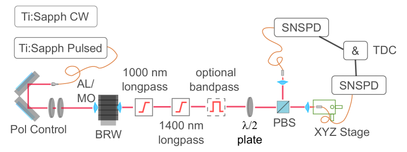
Figure 1: Schematic of the main setup for the pulsed excitation. The selected pump laser is coupled into the waveguide via an aspheric lens (AL) or a microscope objective (MO) on one side and the generated PDC is collected with another AL at the output facet. After collimation, the pump is suppressed by two longpass filters, followed by an optional bandpass. The photon pair is split deterministically at the polarizing beam splitter (PBS) and coupled to fibers via ALs on the XYZ translation stages and detected and correlated subsequently.

We conduct three experiments: The first in section III.1 serves as a sanity check, testing the spatial distribution of the PDC and photoluminescence signals at the facet. Here, we move the collection fiber (single-mode) parallel to the facet to verify that both signals are indeed coming from the waveguide. The second experiment in section III.2 yields a precise model of the PDC and noise. We vary the pump power and employ various bandpass filters after the waveguide while recording the channel rates and coincidences. The final experiment in section III.3 reveals more about the cause of the photoluminescence by measuring the signal power at pump wavelength strongly detuned from the degeneracy point.

For convenience, we operate two almost identical setups according to Fig. 1. In sections III.1 and III.3 we employ a waveguide with a length of $2.04\text{\,}\mathrm{mm}$ and a degeneracy wavelength of $767\text{\,}\mathrm{n}\mathrm{m}$ as well as a microscope objective for the in-coupling. In sections III.2 and III.4 a $1.3\text{\,}\mathrm{mm}$ long waveguide with $763\text{\,}\mathrm{nm}$ degeneracy wavelength is utilized and an aspheric lens is employed for in-coupling. To ensure comparability, both are from the same wafer. These wavelengths are shorter than the design wavelength of $775\text{\,}\mathrm{nm}$. Depending on the location of the chip on the wafer and the waveguide width some variability was observed. We intentionally choose waveguides with shorter operating wavelengths, as they are closer to the bandgap of the material and yield a clearer combined PDC-photoluminescence signal as investigated in section III.3.

The main experimental challenge is keeping all light sources and the setup stable under comparable and reproducible conditions. This imposes a practical limit how much usable data we can actually acquire in a certain time-frame. As some components, like filters, need to be changed for every set, the coupling varies and quick re-alignment is necessary. Therefore, we optimize the setup on metrics that can be derived in real-time in the lab, most importantly the raw coincidence count rate. We operate the setup in a tightly controlled environment suitable for precision interferometry as reported in our Ref. Kauten et al. (2017).

II.2 Rate models for the PDC and photoluminescence

For analysis, we model the observed rates on the detectors (“singles”) as well as the coincidences rates to simultaneously estimate the intrinsic PDC pair production rate and photoluminescence. This approach has been applied to various processes, such as PDC Pearson and Jackson (2010); Schneeloch et al. (2019) or FWM Silverstone et al. (2014); Faruque et al. (2019). In our case, the model is the system of equations,

$$R_{s} =\eta_{s}\left(\xi P+f(P)\right)+R_{\text{bg}},$$ (1)

$$R_{i} =\eta_{i}\left(\xi P+f(P)\right)+R_{\text{bg}}\;\text{and}$$ (2)

$$R_{c} =\eta_{s}\eta_{i}\xi P+\tau_{c}R_{s}R_{i},$$ (3)

which we solve for the detected coincidence rate $R_{c}$. Empirically, we know that the background rate $R_{\text{bg}}$ is equal for both channels, which we include directly in the model. The single rates in Eqs. (1) and (2) are eliminated, allowing us to write $R_{c}$ in terms of the incident optical power $P$, the efficiency to generate photon pairs from that power $\xi$, the heralding efficiencies of “signal” and “idler” $\eta_{s}$ and $\eta_{i}$ according to the Klyshko scheme Klyshko (1980), and the coincidence window $\tau_{c}$. Similar to the intra-waveguide PDC generation rate $\xi P$, the noise model $f(P)$ describes the amount of photoluminescence generated depending on pump power.

A power law is the simplest noise function, which is given by

$$f(P)=\gamma_{P}P^{\alpha},$$ (4)

with $\gamma_{P}$ being the photoluminescence generation efficiency, equivalent to $\xi$. This model is easy to interpret via the exponent $\alpha$ in terms of the number of photons that are involved. If it is dominated by two- or multi-photon processes or exponential avalanche effects, like in laser resonators, the exponent $\alpha$ is greater or equal than $2$. A value of $1$ corresponds to linear absorption, smaller than $1$ indicates saturation.

The second proposed noise function describes a saturable absorber, we assume a “dead-time” model Davidson and Mandel (1968) given by

$$f(P)=\frac{\gamma_{S}P}{1+\beta\gamma_{S}P}.$$ (5)

Here, $\beta$ corresponds to an effective lifetime (or dead-time) of an ensemble of light emitting defects and $\gamma_{S}$ corresponds to $\gamma_{P}$ in Eq. (4). We focus only on these two noise models as others, like ones based on error functions $\propto\text{erf}(P)$ or exponentials $\propto 1-\exp(P)$ fail to converge satisfactorily over the whole power range for the data presented in section III.2.

III Results

III.1 Spatial distribution of the photons at the facet

For start, we determine the spatial distribution of the PDC and background counts of the $2.04\text{\,}\mathrm{mm}$ waveguide. This is done to verify that both coincidences and background originate at the waveguide and are not collected from somewhere else. Moreover, there have been previous hypotheses that the background results from impurities in the GaAs substrate Boitier et al. (2014), which can be verified by comparison with the spatial distribution of the PDC signal.

The collection fiber is held by a clamp mounted on an Elliot Scientific MDE510 fiber launch system. The fiber can be moved in X, Y, and Z-directions relative to the fixed collimating lens. We measure the distribution by moving the fiber in the imaging plane parallel to the waveguide facet. Due to the different focal lengths of the collimating lenses, the image of the waveguide facet is magnified 5.8 times at the plane of the collection fiber.

This approach is limited in resolution by the collection spot size and the difficulty to determine the absolute position of the spot on the facet. The latter can be partially circumvented, as we optimize the coupling for maximum coincidences. According to simulations, the maximum of the coincidences is the center of the ridge and the center of the core layer. We choose this easy to find position as our reference point. First, we scan the distribution of the coincidences, starting with the maximum. Then, we optimize for maximum coincidences again and change the wavelength of the pump lasers, so that no PDC can be detected. This allows us to repeat the same measurement for the photoluminescence using the same reference frame.

In the horizontal direction, which is parallel to the epitaxial layers, both distributions are perfectly centered, but the photoluminescence is much wider. In vertical direction, which is perpendicular to the layers of the BRW structure, the photoluminescence is also wider and the maximum is shifted by approximately $1\text{\,}\mathrm{\SIUnitSymbolMicro m}$ towards the substrate, as shown in Fig. 2. We observe little to no light from the substrate, even though the peak of the photoluminescence is observed slightly shifted towards the substrate. A possible explanation for the wider and shifted emission of the photoluminescence is that there are many modes the impurities can emit into, instead of just the total internal reflection modes for PDC. They may even be only weakly guided and just diffract through the sample, but only the parts that are actually collected are relevant in further experiments.

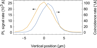
Figure 2: Vertical slice of the photoluminescence signal (orange, left scale) and the coincidences of the PDC (blue, right scale). The peak of the background is slightly below the peak of the PDC coincidences.

The GaAs substrate is semi-insulating, which increases the total number of impurities and potentially the photoluminescence. In contrast to previous hypotheses about the spatial distribution Boitier et al. (2014), our data suggests that the substrate causes little or no relevant photoluminescence. This is important for electrically active samples: If a heavily doped substrate is required to contact the waveguide from below, it will not affect the noise generation rate. Nevertheless, higher doping in the core regions increase the number of impurities, so more photoluminescence has to be expected.

III.2 Rate models from power sweeps at the degeneracy wavelength

In the second experiment, we record the single count rates as well as the coincidences in a $13\text{\,}\mathrm{n}\mathrm{s}$ time window over three orders of magnitude of input power and compare them with the case of narrower temporal time-gating of $1.13\text{\,}\mathrm{n}\mathrm{s}$. The power sweeps are carried out at a pump wavelength of $763\text{\,}\mathrm{n}\mathrm{m}$, which is approximately $0.3\text{\,}\mathrm{nm}$ below the degeneracy wavelength of the employed $1.3\text{\,}\mathrm{mm}$ long waveguide. This wavelength was chosen empirically, as it is a stable and repeatable laser operating point. We select average pump powers with logarithmic spacing between $10\text{\,}\mathrm{\SIUnitSymbolMicro W}$ and $2000\text{\,}\mathrm{\SIUnitSymbolMicro W}$, the typical operating range of our waveguides when pumped externally.

Each power sweep corresponds to one of four conditions: (1) Pulsed pump without filter, (2) pulsed pump with $40\text{\,}\mathrm{n}\mathrm{m}$ or (3) pulsed pump with $12\text{\,}\mathrm{n}\mathrm{m}$ bandpass filter. The bandpass filters are centered at the degeneracy wavelength of the produced signal and idler photons. For condition (4), we remove the bandpass and couple a CW laser into the waveguide. The rationale behind this approach is two-fold: First, the SNSPDs are able to detect light well outside the telecom C-band, we can therefore test the effectiveness of bandpass filtering under pulsed pump conditions. We know from previous measurements that the spectrum of the photoluminescence is very broad and uniform, and that spectral filtering is effective in increasing the signal-to-noise ratio Laiho et al. (2016). Second, the peak power in the pulsed case is roughly $10^{6}$ times higher than in the CW case for the same average power. Any nonlinear effects, like two-photon absorption, should therefore be clearly discernible.

The coefficients of two PDC models with different noise functions are given in table 1, the raw data with power-law fits and with the saturation models are depicted in Fig. 3. For comparison, the analysis with a narrower time gate of $1.13\text{\,}\mathrm{n}\mathrm{s}$ is shown in Fig. 4. Here, only the rate model for the PDC without photoluminescence is fitted. Looking at the data for CW, we suspect that the data point at $20\text{\,}\mathrm{\SIUnitSymbolMicro W}$ is an outlier and is subsequently excluded. Note, that the $12\text{\,}\mathrm{n}\mathrm{m}$ bandpass filter cut way too much signal to get enough data for a sound analysis.

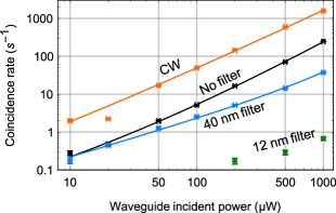
Figure 3: Recorded coincidences with a fit representing the power law and the saturation model for the photoluminescence using a $13\text{\,}\mathrm{n}\mathrm{s}$ window. The two models produce almost identical curves in the displayed range.

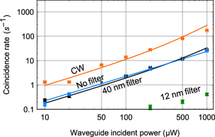
Figure 4: Recorded coincidences using a narrow $1.13\text{\,}\mathrm{n}\mathrm{s}$ window. Here, photoluminescence models are not needed ($f(P)=0$) to explain the curves statistically well enough.

Table 1: Fit coefficients of the two noise models for different pump/filter conditions according to Eqs. (1)-(3). The data measured with the $40\text{\,}\mathrm{n}\mathrm{m}$ bandpass filter can be well explained without a noise model. Most quoted parameter values exhibit a $p$-value of lower than 0.01, except for $\xi$ in the No filter (CW) case and $\beta$ for No filter (pulsed) (both $p=0.1$). The $R^{2}$ is always better than $0.95$. The coincidence window is $13.1\text{\,}\mathrm{n}\mathrm{s}$ (= 1/laser repetition rate), except where stated.

PL model	Parameter	No filter (pulsed)	$40\text{\,}\mathrm{n}\mathrm{m}$ BPF (pulsed)	No filter (CW)
Power law Eq. (4)	$\xi$ ($10^{6}$ pairs/s/µW)	$0.5(1)\text{\,}$	$0.060(1)\text{\,}$	$0.5(2)\text{\,}$
Noise $\propto\gamma_{P}P^{\alpha}$	$\gamma_{P}$ ($10^{6}$ photons/s/µW)	$2.0(4)\text{\,}$	n/a	$8.5(5)\text{\,}$
	$\alpha$	$0.74(4)\text{\,}$	n/a	$0.70(3)\text{\,}$
Saturation Eq. (5)	$\xi$ ($10^{6}$ pairs/s/µW)	$0.78(6)\text{\,}$	$0.060(1)\text{\,}$	$1.40(6)\text{\,}$
Noise $\propto\gamma_{S}P/(1+\beta\gamma_{S}P)$	$\gamma_{S}$ ($10^{6}$ photons/s/µW)	$0.4(1)\text{\,}$	n/a	$2.5(2)\text{\,}$
	$\beta$ (ns)	$8(6)\text{\,}$	n/a	$5(1)\text{\,}$
Short time gate ($1.13\text{\,}\mathrm{n}\mathrm{s}$)	$\xi$ ($10^{6}$ pairs/s/µW)	$0.80(1)\text{\,}$	$0.062(1)\text{\,}$	$1.80(3)\text{\,}$
Klyshko efficiencies	$\eta_{s}\times 10^{-4}$	1.9(1)	4.9(2)	2.6(1)
	$\eta_{i}\times 10^{-4}$	1.5(1)	8.5(3)	3.2(1)

We then take a closer look at the estimated PDC pair generation rates $\xi$. As the setup and waveguide remain identical in between experiments, these values speak for the consistency of our measurements. Most of the rates are within the range of $5\text{\times}{10}^{5}\text{\,}\mathrm{p}\mathrm{a}\mathrm{i}\mathrm{r}\mathrm{s}\mathrm{/}\mathrm{\SIUnitSymbolMicro}\mathrm{W}\mathrm{/}\mathrm{s}8\text{\times}{10}^{5}\text{\,}\mathrm{p}\mathrm{a}\mathrm{i}\mathrm{r}\mathrm{s}\mathrm{/}\mathrm{\SIUnitSymbolMicro}\mathrm{W}\mathrm{/}\mathrm{s}$ without filters, and an order of magnitude less with a $40\text{\,}\mathrm{n}\mathrm{m}$ bandpass filter. The only exception is the saturation model in the No filter (CW) case, which reports pair rates more than twice as high as the other cases. This might be an artifact of the low dead-time it converged to. Because of the known repetition rate, we expect an effective dead-time slightly above $10\text{\,}\mathrm{n}\mathrm{s}$.

However, this raises the question of whether a reduction to a tenth of the PDC rate is agreeable when employing $40\text{\,}\mathrm{n}\mathrm{m}$ bandpass filter. As the spectrum of the PDC is more than $90\text{\,}\mathrm{n}\mathrm{m}$ FWHM wide Günthner et al. (2015), a considerable reduction in power can already be expected. Including the transmission profile of the filter, we determine that only approximately $32\text{\,}\mathrm{\char 37\relax}$ of the signal/idler photons are transmitted, while the rest is absorbed or reflected by the filter. As coincidence rates are affected twice, due to the involvement of two correlated photons, the total PDC transmission is expected to be about $10\text{\,}\mathrm{\char 37\relax}$, which is consistent with our results for the PDC rates.

Moreover, as the noise is spectrally broader than the PDC Laiho et al. (2016), the signal-to-noise ratio increases. This is evident as the model without photoluminescence ($\gamma_{S}$ or $\gamma_{P}=0$) yields a statistically significant fit in Table 1.

Our results show that the exponents of the photoluminescence power law model are significantly below 1. This indicates that the driving factor of the photoluminescence is saturable linear absorption, and that higher-order photon processes play only marginal roles in our experimental conditions. In the following section III.3, the dependence of the photoluminescence generation rates on the pump wavelength supports this hypothesis. The saturation is modeled as an excitation with a lifetime, which assumes that the photoluminescence stems from impurities that can only be re-excited after a delay when emitting a photon.

We emphasize that the photoluminescence scale factors $\gamma_{S}$ and $\gamma_{P}$ serve the same purpose, but their values cannot be compared directly without taking $f(P)$ into account. The true rate is only given by $f(P)$. For example, at high powers $f(P)$ predicts a much higher photoluminescence rate for the saturation model compared to the power model. At low powers it is vice-versa. Both models can explain the overall shape of the curves well and statistically sound. Further discussions about the differences are given in section III.4 and Fig. 7.

Note, that the Klyshko efficiencies are two orders of magnitude lower as in our previous work, which is caused by the nature of this experiment. As we are deliberately trying to measure the photoluminescence, we refrain from tight spatial, temporal or spectral filtering. Hence, the single rates increase by a large amount, while the coincidence rates stay relatively low. In our previous work Günthner et al. (2015), we report up to $\eta\sim$6\text{\,}\mathrm{\char 37\relax}$$ by employing the proper filters.

III.3 Off-resonant photoluminescence generation rates

In the final experiment, we move the excitation wavelength away from the degeneracy point, mostly towards longer wavelengths where no PDC is produced, because the phasematching condition is no longer fulfilled. On occasion, we have observed PDC processes of various types that probably involve higher-order modes in several waveguides. We avoid these wavelengths in this experiment to focus solely on the photoluminescence. We measure the magnitude and linearity of the photoluminescence at each wavelength for different excitation powers.

In this section, we employ the setup with the microscope objective and the sample with a length of $2.04\text{\,}\mathrm{mm}$ (degeneracy wavelength $767\text{\,}\mathrm{n}\mathrm{m}$). We use a $40\text{\,}\mathrm{n}\mathrm{m}$ bandpass filter and a pulsed pump to emulate the conditions for a typical broadband PDC experiment with BRWs.

Without the PDC, we neglect coincidences so the full rate model is no longer necessary. Instead, we simply record the rates on one of the SNSPDs, measuring only dark counts plus the photoluminescence. This can be described by a power law with an offset

$$R_{s}(P)=AP^{\alpha}+R_{\text{0}},$$ (6)

where $P$ is the power before the waveguide in-coupling objective. The scale factor of the polynomial $A$ can be interpreted as the photoluminescence generation rate, $R_{0}$ is the count rate at the lowest power measured, including dark-counts and background. The exponent $\alpha$ corresponds to the one from the fits and models discussed in the previous section III.2, but is determined independently for each photoluminescence data set. This model shows an excellent agreement with the measured data in Fig. 5. The resulting fit coefficients are listed in table 2. We find that $\alpha$ is very close to one, with the tendency that shorter wavelengths slightly deviate towards lower exponents. This is a further hint at saturation effects, which are more noticeable the closer the excitation wavelength is to the bandgap of the materials. We note that the value of the exponent can only be compared qualitatively between samples. The exact nature, realisation and excitation of the impurities can vary between the waveguides, resulting in slightly different rates and exponents.

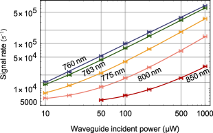
Figure 5: Raw data of the off-resonant photoluminescence generation rates at telecom wavelengths for different average excitation powers and pump wavelengths between $760\text{\,}\mathrm{n}\mathrm{m}$ and $850\text{\,}\mathrm{n}\mathrm{m}$. The data is fitted with the power law from Eq. (6). The fit parameters are listed in Table 2, the generation rate $A$ is plotted in Fig. 6.

Table 2: Fit coefficients of the power law with offset from Eq. (6).

Wavelength	$A$ ($\mathrm{p}\mathrm{h}\mathrm{o}\mathrm{t}\mathrm{o}\mathrm{n}\mathrm{s}\mathrm{/}\mathrm{\SIUnitSymbolMicro}\mathrm{W}\mathrm{/}\mathrm{s}$)	$\alpha$	$R_{0}$ ($\mathrm{p}\mathrm{h}\mathrm{o}\mathrm{t}\mathrm{o}\mathrm{n}\mathrm{s}\mathrm{/}\mathrm{s}$)
760 $\mathrm{n}\mathrm{m}$	1800(300)	0.86(3)	$100(1400)\text{\,}$
763 $\mathrm{n}\mathrm{m}$	1130(150)	0.91(3)	$3000(1000)\text{\,}$
775 $\mathrm{n}\mathrm{m}$	360(50)	1.00(2)	$4400(400)\text{\,}$
800 $\mathrm{n}\mathrm{m}$	87(13)	1.07(3)	$5000(140)\text{\,}$
850 $\mathrm{n}\mathrm{m}$	27(10)	1.00(6)	$4200(300)\text{\,}$

The photoluminescence generation rate $A$ (table 2) shows a distinct behaviour in Fig. 6. Over the span of $100\text{\,}\mathrm{n}\mathrm{m}$ above the bandgap, it decreases by two orders of magnitude. To model this behaviour, we tried a variety of functions, like polynomials or exponentials similar to the overlap integrals known from solid state physics Gross and Marx (2014). It turns out, the only viable model is a Lorentzian function given by

$$A(h\nu)=\frac{\mathcal{N}}{1+\left(\frac{h\nu-E_{g}}{\sigma}\right)^{2}}.$$ (7)

While $\mathcal{N}$ and $\sigma$ are just scale parameters, the position of the resonance, $E_{g}=$1.654(4)\text{\,}\mathrm{e}\mathrm{V}$\approx$750\text{\,}\mathrm{n}\mathrm{m}$$, can be explained physically: Its value is very close to the bandgap of the matching layers with an aluminum concentration of nominally $20\text{\,}\mathrm{\char 37\relax}$. The Lorentzian function is an excellent approximation for the real and imaginary parts of the dielectric function near the bandgap of Al_xGa_1-xAs alloys with an aluminum concentration of $x$ Kim et al. (1993). In the literature, the quoted bandgap of Al_xGa_1-xAs varies slightly Kim et al. (1993); Gehrsitz et al. (2000); Adachi (1993). If we also take the typical fabrication error of the concentration of about two percentage points into account, our estimation of $E_{g}$ corresponds to an aluminum concentration of $18.5\text{\,}\mathrm{\char 37\relax}19.5\text{\,}\mathrm{\char 37\relax}$, which is well within the manufacturing specification. Together with the rate modeling from the previous section III.2, this strongly indicates that linear absorption is indeed the driving factor of the photoluminescence.

Figure 6: Noise generation rate $A$ from table 2 with Lorentzian fit according to Eq. (7). The resonance is centered at $1.654(4)\text{\,}\mathrm{e}\mathrm{V}$ ($750\text{\,}\mathrm{n}\mathrm{m}$), which is approximately the bandgap of the matching layer materials.

III.4 Considerations for future devices

Identifying and modelling the driving factors of the photoluminescence allows us to improve future samples. The first and foremost measure is increasing the spread between the lowest bandgap and the design wavelength. We propose two measures to reduce the noise: longer operating wavelengths and lower bandgap materials.

Quantitatively, we can estimate the effect of these proposals for the sample at hand from the fit in Fig. 6. First, moving from a $767\text{\,}\mathrm{n}\mathrm{m}$ to a $780\text{\,}\mathrm{n}\mathrm{m}$ pump wavelength already reduces the amount of photoluminescence by $70\text{\,}\mathrm{\char 37\relax}$. Second, our powerful automated sample design suite Pressl et al. (2017) allows us to easily modify the sample to increase the aluminum concentration. For example, changing just the two matching layers next to the core from a concentration of $20\text{\,}\mathrm{\char 37\relax}$ to $22\text{\,}\mathrm{\char 37\relax}$, reduces the photoluminescence by another $60\text{\,}\mathrm{\char 37\relax}$. Both measures increase the spread between excitation and bandgap edge and result in a $90\text{\,}\mathrm{\char 37\relax}$ total reduction compared to the samples investigated here. It is important to note that these small changes do not affect the critical performance metrics Pressl et al. (2017) of the waveguide, like the mode overlap and the effective nonlinearity.

Furthermore, since we now have the full rate model description (Eqs. (1)-(3) and Table 1) of our $1.3\text{\,}\mathrm{m}\mathrm{m}$ long waveguide at hand, we calculate the coincidence-to-accidentals ratio (CAR) curves for different filters and potential alternative designs, which may have modified material compositions, other geometries or shifted design wavelengths. A great advantage of this model-based approach is the separation of the PDC and noise signal. This allows us to evaluate the effects of different coincidence windows on the figures of merit.

The results for two different coincidence windows are depicted in Fig. 7. It is clearly visible that spectral filtering and time filtering prove to be highly effective, as a model without photoluminescence can explain the measured data well. A narrow time gate increases the maximum CAR by a factor of 10. Without spectral filter, a noise-optimized design could increase the usable pump power substantially for a fixed CAR. The saturation model without spectral filters (solid blue line) in Fig. 7 yields a CAR of 7 at $100\text{\,}\mathrm{\SIUnitSymbolMicro W}$ pump power. Keeping the CAR constant and moving to the dashed line representing a sample with $90\text{\,}\mathrm{\char 37\relax}$ reduction in the photoluminescence, shows a pump power of around $200\text{\,}\mathrm{\SIUnitSymbolMicro W}$ - which corresponds to doubling the pair rate.

Furthermore, it is clearly visible that both noise models have their merits. We believe the power law in Eq. (4) provides a good estimate of the PDC production rate, while the saturation model in Eq. (5) provides a good description of the processes at lower powers. The slight discrepancy with the measured data, however, also shows that we still cannot capture the full physics of our system. Moreover, the fact that two parameters in Table 1 could only be fitted to a $p$-value of 0.1 indicates the limitations of the statistics and the models in certain cases. Building the model from a pure quantum optics approach, i.e. mean photon numbers, failed to produce reliable results over the whole power range.

We emphasize that the values reported in Fig. 7 are conservative in the sense that we did not explicitly align for maximum CAR. Properly optimizing the pumping and coupling, also in connection with narrower filtering (e.g. $12\text{\,}\mathrm{n}\mathrm{m}$ bandpass), yields values at least an order of magnitude higher Chen et al. (2018). This can be seen instantly as the graph for $90\text{\,}\mathrm{\char 37\relax}$ reduction is not even close to the $40\text{\,}\mathrm{n}\mathrm{m}$ case, which it should be. With better alignment, however, there is much headroom for optimizing for the individual case. Nevertheless, it follows that for these hypothetical samples, the filtering requirements are relaxed significantly compared to the state-of-the-art. This can be especially interesting for any integrated detection system: Realizing high fidelity time filtering to the picosecond level is much harder than just to nanoseconds. This is also true for on-chip spectral bandpass filters.

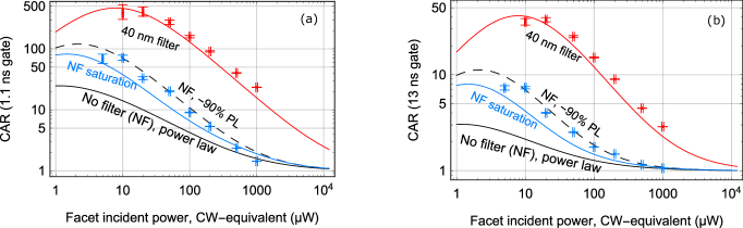
Figure 7: Predicted CAR values for different conditions with a pulsed pump at $76.2\text{\,}\mathrm{MHz}$ repetition rate. At low powers, the CAR is limited by the dark counts of the detectors ($300\text{\,}{\mathrm{s}}^{-1}$), at high powers by the accidental coincidences. Both the raw data (symbols) from Figs. 3 and 4 and curves derived from the different models ($40\text{\,}\mathrm{n}\mathrm{m}$, red and No filter, black and blue) are shown. The black solid line depicts the no filter power law model, while the blue line is the corresponding saturation model, showing better agreement to the measurements, especially at low powers. The dashed line is a hypothetical sample, with the photoluminescence reduced by $90\text{\,}\mathrm{\char 37\relax}$. Here, choosing either the power law or saturation model made no significant difference. Fig. (a) shows the time filtered case with a $1.13\text{\,}\mathrm{n}\mathrm{s}$ time gate, (b) the unfiltered with $13.1\text{\,}\mathrm{n}\mathrm{s}$. Note that the vertical scales are different by an order of magnitude.

Having the full model depending on the input power allows us not only to estimate the CAR, but also to predict pair rates for an on-chip pump and photonic network. As all the stated input powers are measured before the aspheric lens, we need to determine the individual loss factors for coupling into the waveguide. The actual power guided in the pump mode can be recovered by multiplying the aspheric lens transmission ($70\text{\,}\mathrm{\char 37\relax}$) with the total in-coupling efficiency ($<$$35\text{\,}\mathrm{\char 37\relax}$) and the typical relative pump mode excitation ($>$$4\text{\,}\mathrm{\char 37\relax}$) Pressl et al. (2015). Thus, only $1\text{\,}\mathrm{\char 37\relax}$ of the power reaches the necessary pump mode. Hence, we estimate that the true coefficient of pair generation rate, e.g. for an on-chip pump, is in fact on the order of $5\text{\times}{10}^{7}\text{\,}{\mathrm{\SIUnitSymbolMicro W}}^{-1}\text{\,}{\mathrm{s}}^{-1}$. In a pure externally pumped system, this is not achievable due to absorption of the glass in the objective, even with proper beam shaping to match the far field mode shape. In contrast, an active, electrically pumped, waveguide laser runs intrinsically in the correct mode Bijlani et al. (2013); Boitier et al. (2014). This means that for $1\text{\,}\mathrm{mW}$ of internal laser power, a pair rate of at least $5\text{\,}\mathrm{GHz}$ can be expected. Such rates are tremendously useful as they can be harnessed by a fully integrated (quantum) optic network.

IV Conclusion

We have presented three different measurements designed to gain insight into the nature of BRW photoluminescence. We proposed two rate models to describe the photon generation process from a big-picture point of view. There is strong evidence that the main cause of photoluminescence is electron-hole pair excitation via linear absorption of a pump photon, followed by a short lived radiative decay via deep impurity levels. The defects that provide these deep levels are located in the matching layers with a low aluminum concentration right next to the core. Furthermore, we have proposed small modifications in the sample design that promise to greatly reduce the photoluminescence. Our calculations predict a reduction by $90\text{\,}\mathrm{\char 37\relax}$, while promising high non-linearity and photon pair rates in the GHz regime.

Author contributions

Conceptualization, S.A., K.L., B.P., G.W.; Formal analysis, S.A., B.P.; Methodology, S.A., A.S., K.L., B.P, G.W.; Investigation, S.A., A.S., K.L. B.P., H.T.; Resources, H.S., M.K., S.H., C.S.; Software, B.P.; Supervision, B.P., G.W.; Writing - original draft, S.A., B.P.; Writing - review & editing, A.S., K.L., H.T., C.S., G.W.; Funding acquisition, C.S., G.W.;

References

References

- O’Brien (2007) J. L. O’Brien, Science 318, 1567 (2007).
- Rudolph (2017) T. Rudolph, APL Photonics 2, 030901 (2017).
- Ma et al. (2012) X.-S. Ma, T. Herbst, T. Scheidl, D. Wang, S. Kropatschek, W. Naylor, B. Wittmann, A. Mech, J. Kofler, E. Anisimova, V. Makarov, T. Jennewein, R. Ursin, and A. Zeilinger, Nature 489, 269 (2012).
- Günthner et al. (2017) K. Günthner, I. Khan, D. Elser, B. Stiller, O. Bayraktar, C. R. Müller, K. Sauke, D. Tröndle, F. Heine, S. Seel, P. Greulich, H. Zech, B. Gütlich, I. Richter, M. Lutzer, S. Philipp-May, R. Meyer, C. Marquardt, and G. Leuchs, Optica 4, 611 (2017).
- Aspect et al. (1981) A. Aspect, P. Grangier, and G. Roger, Physical Review Letters 47, 460 (1981).
- Kwiat et al. (1995) P. G. Kwiat, K. Mattle, H. Weinfurter, A. Zeilinger, A. V. Sergienko, and Y. Shih, Physical Review Letters 75, 4337 (1995).
- Patel et al. (2012) K. A. Patel, J. F. Dynes, I. Choi, A. W. Sharpe, A. R. Dixon, Z. L. Yuan, R. V. Penty, and A. J. Shields, Physical Review X 2, 041010 (2012).
- Eraerds et al. (2010) P. Eraerds, N. Walenta, M. Legré, N. Gisin, , and H. Zbinden, New Journal of Physics 12, 063027 (2010).
- Schweickert et al. (2018) L. Schweickert, K. D. Jöns, K. D. Zeuner, S. F. C. da Silva, H. Huang, T. Lettner, M. Reindl, J. Zichi, R. Trotta, A. Rastelli, and V. Zwiller, Applied Physics Letters 112, 093106 (2018).
- Shields (2007) A. J. Shields, Nature Photonics 1, 215 (2007).
- Brassard et al. (2000) G. Brassard, N. Lütkenhaus, T. Mor, and B. C. Sanders, Physical Review Letters 85, 1330 (2000).
- Politi et al. (2008) A. Politi, M. J. Cryan, J. G. Rarity, S. Yu, and J. L. O’Brien, Science 320, 646 (2008).
- Armengol et al. (2008) J. M. P. Armengol, B. Furch, C. J. de Matos, O. Minster, L. Cacciapuoti, M. Pfennigbauer, M. Aspelmeyer, T. Jennewein, R. Ursin, T. Schmitt-Manderbach, G. Baister, J. Rarity, W. Leeb, C. Barbieri, H. Weinfurter, and A. Zeilinger, Acta Astronautica 63, 165 (2008).
- Yin et al. (2017) J. Yin, Y. Cao, Y. H. Li, S. K. Liao, L. Zhang, J. G. Ren, W. Q. Cai, W. Y. Liu, B. Li, and H. Dai, Science 356, 1140 (2017).
- Lanco et al. (2006) L. Lanco, S. Ducci, J.-P. Likforman, X. Marcadet, J. Van Houwelingen, H. Zbinden, G. Leo, and V. Berger, Phys. Rev. Lett. 97, 173901 (2006).
- Sarrafi et al. (2013) P. Sarrafi, E. Y. Zhu, K. Dolgaleva, B. M. Holmes, D. C. Hutchings, J. S. Aitchison, and L. Qian, Appl. Phys. Lett. 103, 251115 (2013).
- Horn et al. (2012) R. Horn, P. Abolghasem, B. J. Bijlani, D. Kang, A. S. Helmy, and G. Weihs, Phys. Rev. Lett. 108, 153605 (2012).
- Boyd (2003) R. W. Boyd, Nonlinear Optics (Academic Press, 2003).
- Pressl et al. (2015) B. Pressl, T. Günthner, K. Laiho, J. Geßler, M. Kamp, S. Höfling, C. Schneider, and G. Weihs, Opt. Express 23, 33608 (2015).
- Porkolab et al. (2014) G. A. Porkolab, P. Apiratikul, B. Wang, S. H. Guo, and C. J. K. Richardson, Opt. Express 22, 7733 (2014).
- Pressl et al. (2017) B. Pressl, K. Laiho, H. Chen, T. Günthner, A. Schlager, S. Auchter, H. Suchomel, M. Kamp, S. Höfling, C. Schneider, and G. Weihs, Quantum Sci. Technol. 3, 024002 (2017).
- Günthner et al. (2015) T. Günthner, B. Pressl, K. Laiho, J. Geßler, S. Höfling, M. Kamp, C. Schneider, and G. Weihs, J. Opt. 17, 125201 (2015).
- Autebert et al. (2016) C. Autebert, J. Trapateau, A. Orieux, A. Lemaître, C. Gomez-Carbonell, E. Diamanti, I. Zaquine, and S. Ducci, Quantum Sci. Technol. 1, 01LT02 (2016).
- Kang et al. (2016) D. Kang, A. Anirban, and A. S. Helmy, Opt. Express 24, 15160 (2016).
- Boitier et al. (2014) F. Boitier, A. Orieux, C. Autebert, A. Lemaître, E. Galopin, C. Manquest, C. Sirtori, I. Favero, G. Leo, and S. Ducci, Phys. Rev. Lett. 112, 183901 (2014).
- Bijlani et al. (2013) B. J. Bijlani, P. Abolghasem, and A. S. Helmy, Appl. Phys. Lett. 103, 091103 (2013).
- Vallés et al. (2013) A. Vallés, M. Hendrych, J. Svozilík, R. Machulka, P. Abolghasem, D. Kang, B. J. Bijlani, A. S. Helmy, and J. P. Torres, Opt. Express 21, 10841 (2013).
- Horn et al. (2013) R. T. Horn, P. Kolenderski, D. Kang, P. Abolghasem, C. Scarcella, A. Della Frera, A. Tosi, L. G. Helt, S. V. Zhukovsky, J. E. Sipe, et al., Sci. Rep. 3, 2314 (2013).
- Kang et al. (2015) D. Kang, M. Kim, H. He, and A. S. Helmy, Phys. Rev. A 92, 013821 (2015).
- Schlager et al. (2017) A. Schlager, B. Pressl, K. Laiho, H. Suchomel, M. Kamp, S. Höfling, C. Schneider, and G. Weihs, Opt. Lett. 42, 2102 (2017).
- Machulka et al. (2014) R. Machulka, K. Lemr, O. Haderka, M. Lamperti, A. Allevi, and M. Bondani, Journal of Physics B: Atomic, Molecular and Optical Physics 47, 215501 (2014).
- Bhar et al. (1989) G. C. Bhar, S. Das, and U. Chatterjee, Appl. Opt. 28, 202 (1989).
- Chen et al. (2009) J. Chen, A. J. Pearlman, A. Ling, J. Fan, and A. Migdall, Opt. Express 17, 6727 (2009).
- Zhu et al. (2011) E. Y. Zhu, Z. Tang, E. A. L. Kim-Koon, L. Qian, L. G. Helt, M. Liscidini, J. E. Sipe, C. Corbari, A. Canagasabey, M. Ibsen, and P. G. Kazansky, in Advanced Photonics (Optical Society of America, 2011) p. SOWC3.
- Takesue and Inoue (2005) H. Takesue and K. Inoue, Opt. Express 13, 7832 (2005).
- Yuan et al. (2002) Z. Yuan, B. E. Kardynal, R. M. Stevenson, A. J. Shields, C. J. Lobo, K. Cooper, N. S. Beattie, D. A. Ritchie, and M. Pepper, Science 295, 102 (2002).
- Stevenson et al. (2006) R. M. Stevenson, R. J. Young, K. C. P. Atkinson, D. A. Ritchie, and A. J. Shields, Nature 439, 179 (2006).
- Christ et al. (2013) A. Christ, B. Brecht, W. Mauerer, and C. Silberhorn, New Journal of Physics 15, 053038 (2013).
- Pavesi and Guzzi (1994) L. Pavesi and M. Guzzi, Journal of Applied Physics 75, 4779 (1994).
- Laiho et al. (2016) K. Laiho, B. Pressl, A. Schlager, H. Suchomel, M. Kamp, S. Höfling, C. Schneider, and G. Weihs, Nanotechnology 27, 434003 (2016).
- Chen et al. (2018) H. Chen, S. Auchter, M. Prilmüller, A. Schlager, T. Kauten, K. Laiho, B. Pressl, H. Suchomel, M. Kamp, S. Höfling, C. Schneider, and G. Weihs, APL Photonics 3, 080804 (2018).
- Kauten et al. (2017) T. Kauten, R. Keil, T. Kaufmann, B. Pressl, Č. Brukner, and G. Weihs, New J. Phys 19, 033017 (2017).
- Pearson and Jackson (2010) B. J. Pearson and D. P. Jackson, American Journal of Physics 78, 471 (2010).
- Schneeloch et al. (2019) J. Schneeloch, S. H. Knarr, D. F. Bogorin, M. L. Levangie, C. C. Tison, R. Frank, G. A. Howland, M. L. Fanto, and P. M. Alsing, Journal of Optics 21, 043501 (2019), arXiv:1807.10885 .
- Silverstone et al. (2014) J. W. Silverstone, D. Bonneau, K. Ohira, N. Suzuki, H. Yoshida, N. Iizuka, M. Ezaki, C. M. Natarajan, M. G. Tanner, R. H. Hadfield, et al., Nature Photonics 8, 104 (2014).
- Faruque et al. (2019) I. I. Faruque, G. F. Sinclair, D. Bonneau, T. Ono, C. Silberhorn, M. G. Thompson, and J. G. Rarity, Phys. Rev. Applied 12, 054029 (2019).
- Klyshko (1980) D. N. Klyshko, Sov. J. Quantum Electron. 12, 1112 (1980).
- Davidson and Mandel (1968) F. Davidson and L. Mandel, Journal of Applied Physics 39, 62 (1968), https://doi.org/10.1063/1.1655781 .
- Gross and Marx (2014) R. Gross and A. Marx, Festkörperphysik, De Gruyter Studium (De Gruyter, 2014).
- Kim et al. (1993) C. C. Kim, J. W. Garland, and P. M. Raccah, Physical Review B 75, 4779 (1993).
- Gehrsitz et al. (2000) S. Gehrsitz, F. Reinhart, C. Gourgon, N. Herres, A. Vonlanthen, and H. Sigg, J. Appl. Phys. 87, 7825 (2000).
- Adachi (1993) S. Adachi, Properties of aluminium gallium arsenide, edited by S. Adachi, No. 7 (Inspec, London, 1993).