Inflation, ECB and short-term interest rates:
A new model, with calibration to market data

Abstract

We propose a new model for the joint evolution of the European inflation rate, the European Central Bank official interest rate and the short-term interest rate, in a stochastic, continuous time setting.

We derive the valuation equation for a contingent claim and show that it has a unique solution. The contingent claim payoff may depend on all three economic factors of the model and the discount factor is allowed to include inflation.

Taking as a benchmark the model of Ho, H.W., Huang, H.H. and Yildirim, Y., Affine model of inflation-indexed derivatives and inflation risk premium, European Journal of Operational Research, 2014, we show that our model performs better on market data from 2008 to 2015.

Our model is not an affine model. Although in some special cases the solution of the valuation equation might admit a closed form, in general it has to be solved numerically. This can be done efficiently by the algorithm that we provide. Our model uses many fewer parameters than the benchmark model, which partly compensates the higher complexity of the numerical procedure and also suggests that our model describes the behaviour of the economic factors more closely.

Keywords. Inflation, interest rates, inflation-linked derivatives, risk-neutral valuation

JEL Classification. C02 $\cdot$ G12 $\cdot$ C6

MSC 2010 Classification. 91B28 $\cdot$ 91B24 $\cdot$ 35D40

1 Introduction

The issuance of sovereign bonds linked to euro area inflation began with the introduction of bonds indexed to the French consumer price index (CPI) excluding tobacco (Obligations Assimilables du Trésor indexées or OATis) in 1998. In 2003, Greece, Italy and Germany decided to issue inflation-linked bonds too, and nowadays a variety of inflation-linked derivatives are quoted in European financial markets. Typical examples are inflation indexed swaps, which allow to exchange the inflation rate for a fixed interest rate, or inflation caps, which pay out if the inflation exceeds a certain threshold over a given period (for a detailed introduction to inflation derivatives, see e.g. [DDM04]).

The pricing of inflation-linked derivatives is related to both interest rate and foreign exchange theory. In their seminal work of 2003, Jarrow and Yildirim [JY03] proposed an approach based on foreign currency and interest rate derivatives valuation. On the other hand, there is some empirical and theoretical evidence that bond prices, inflation, interest rates, monetary policy and output growth are related. In particular, both inflation and interest rates are clearly related to the activity of central banks.

In the present work we propose a model for the joint evolution of the European inflation rate, the European Central Bank (henceforth ECB) official interest rate and the short-term interest rate, and use it to price European type derivatives whose payoff depends potentially on all three factors. To the best of our knowledge, ours is the first model that takes into account the interaction among all these three factors. With the 2007-2008 financial crisis it has become clear that there is another risk factor underlying bond prices, namely credit risk, but we leave the construction of a model that incorporates this factor for future work.

Our model is a stochastic, continuous time one. More precisely, the ECB interest rate evolves as a pure jump process with jump intensity and distribution that depend both on its current value and on the current value of inflation. As inflation is measured at regular times, the inflation rate is modeled as a piecewise constant process that jumps at fixed times $t_{i}$. The new value at $t_{i}$ is given by a Gaussian random variable with expectation depending on the previous value of the inflation rate and on the current value of the ECB interest rate. Finally, the short-term interest rate follows a CIR type model with reversion towards an affine function of the ECB interest rate and diffusion coefficient depending on the spread between itself and the ECB interest rate.

Many models proposed to price inflation indexed derivatives fall in the class of affine models (see e.g. D’Amico, Kim and Wei [DKW18], Ho, Huang and Yildirim [HHY14] and Waldenberger [W17]). Singor et al. [SGVBO13] consider a Heston-type inflation model in combination with a Hull-White model for interest rates, with non-zero correlations. Hughston and Macrina [HM08] propose a discrete time model based on utility functions. Haubric et al. [HPR12] develop a discrete time model of nominal and real bond yield curves based on several stochastic drivers.

Our model does not fall within the class of affine models, and does not reduce to other known models. Therefore a certain amount of mathematical work is needed to study it, in particular to derive the valuation equation for the price of a derivative and to show that it has a unique solution. In fact the proof relies on a general result by Costantini, Papi and D’Ippoliti [CPD12] on valuation equations for jump-diffusion underlyings. The derivative payoff may depend on all three economic factors of the model and the discount factor is allowed to include inflation (see Remark 3.1). Although in some special cases the price might admit a closed form, or might be approximated by a closed form, in general it has to be computed numerically. This can be done efficiently by the numerical algorithm described in Appendix C.

In order to show that the higher complexity of the numerical implementation of our valuation model is justified, we compare our valuation model to the well known model of D’Amico, Kim and Wei [DKW18] and Ho, Huang and Yildirim [HHY14]). The improvement in the error measures is significant (see Tables 1 and 2). Note that our model requires many fewer parameters than the Ho, Huang ad Yildirim model, which compensates the higher complexity of the numerical implementation, at least partly. Moreover, the fact that our model performs better than the Ho, Huang and Yildirim model with many fewer parameters suggests that it describes more closely the behaviour of the economic factors.

The paper is organized as follows. In Section 2, we introduce the mathematical model. In Section 3 we derive the valuation equation. Proofs are postponed to Appendix B. The general result by Costantini, Papi and D’Ippoliti [CPD12] is recalled in Appendix A. In Section 4 we compare our model to the model of [HHY14]: We calibrate both models to the market prices of Zero Coupon Inflation Indexed Swaps from January 2008 to October 2015 and measure the performances of the two models in fitting the market data (Table 1). We also carry out the same analysis for the period 2008-2011, when, due to the subprime crisis, interest rates dropped drastically and rapidly (Table 2). In both periods there is a significant improvement in the error measures.

2 The model

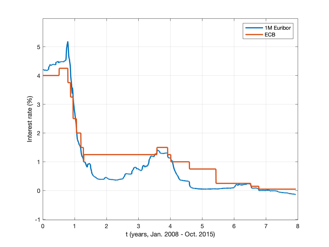
Figure 1: Evolution of the official European Central Bank interest rate and the Euribor interest rate from January 2008 to October 2015.

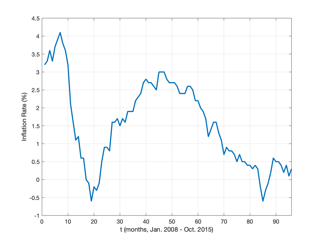
Figure 2: Evolution of the European inflation rate from January 2008 to October 2015.

Figure 1 plots the ECB interest rate together with the Euribor interest rate between 2008 and 2015, while figure 2 plots inflation in the same period. The primary goal of the ECB is to maintain price stability, i.e., to keep inflation within a desired range (close to 2%). The inflation target is achieved through periodic adjustments of the ECB official interest rate and, consequently, of the short-term interest rate. The goal of this paper, and specifically of this section, is to formulate a dynamical model that describes the interactions among inflation, the ECB and the short-term interest rates.

From now on, we fix the probability space $\left(\Omega,\mathcal{F},\mathbb{P}\right)$, where $\mathbb{P}$ is a martingale measure.

2.1 European Inflation

European inflation data are officially made known once a month, hence we model the inflation rate as a stochastic process that jumps at fixed times, with jump sizes depending on its previous value and on the official ECB interest rate, and is constant between two jumps.
Specifically, with the usual convention that one year is an interval of length one, let $\mathcal{T}:=\{t_{i}\}_{i\geq 0,\ldots,M}$ be the sequence of times at which the values of the inflation rate process $\left\{\Pi(t_{i})\right\}_{t_{i}\in\mathcal{T}}$ are observed, where $t_{0}=0$, $t_{1}=\frac{1}{12}$ and, for $i\geq 2$, $t_{i}=it_{1}$.
The evolution is then given by

$$\left\{\begin{array}[]{ll}\Pi(0)=\Pi_{0},\\ \Pi(t)=\Pi(t_{i}),&\quad t_{i}\leq t<t_{i+1},\\ \Pi(t_{i+1})=\gamma\left(\Pi(t_{i}),R(t_{i+1}^{-})\right)+\epsilon_{i+1},&\quad t=t_{i+1},\end{array}\right.$$ (2.1)

where $\gamma$ is a linear function defined by

$$\gamma(\pi,r)=\alpha\pi+k^{\Pi}(\pi^{*}-\pi)+\beta\,r=(\alpha-k^{\Pi})\pi+k^{\Pi}\pi^{*}+\beta\,r,$$ (2.2)

with $\alpha,\leavevmode\nobreak\ \beta\in\mathbb{R}$ and $k^{\Pi},\leavevmode\nobreak\ \pi^{*}\in\mathbb{R}_{+}$ constant parameters such that $0<\alpha-k^{\Pi}<1$.
The fluctuations $\{\epsilon_{i}\}_{i=1,\ldots,M}$ are i.i.d. random variables distributed according to the $\mathcal{N}(0,v^{2})$ law, and $R(t)$, for $t\in[0,T]$, is the interest rate process which will be described in Section 2.2.
We can see that

$$\gamma(\pi,r)=\pi+\left(k^{\Pi}-\alpha+1\right)\left[\frac{k^{\Pi}\pi^{*}+\beta\,r}{k^{\Pi}-\alpha+1}-\pi)\right]$$ (2.3)

and hence the condition $0<\alpha-k^{\Pi}<1$ yields that the process $\Pi$ satisfies the mean-reversion property towards $\frac{k^{\Pi}\pi^{*}+\beta\,r}{k^{\Pi}-\alpha+1}$.

2.2 European Central Bank Interest Rate

Looking at figure 1, we can recognise some important facts about the ECB interest rate. The level of the rate is persistent, hence the sample path is a step function; The changes are multiples of 25 basis points (bp); A change is often followed by additional changes, frequently in the same direction. Therefore we model the ECB interest rate, $R(t)$, as a continuous time, pure jump process with finitely many possible upward and downward jump values. These jumps occur at random times $\{\vartheta_{i}\}$, and their size is equal to $k\delta$ with $\delta=0.0025$ and $k\in\{-m,...,-1,1,...,m\}$. The jump intensity, $\lambda$, is a function of the current values of inflation and the ECB interest rate (when the level of the official interest rate is low, there is a tendency to avoid further downward jumps). The probability of occurence of a jump $k\delta$ also depends upon the current values of inflation and the ECB interest rate, i.e. it is a function $p(\pi,r,k\delta)$.

Since, by definition, an interest rate is always larger than -1, we can assume,without loss of generality, $R(t)>\underline{r},\quad\underline{r}\geq-1$ , for all $t>0$. In addition, we suppose that there exists a maximum value $0<\overline{r}<+\infty$ such that $R(t)<\overline{r},$ for all $t>0.$ Consistently we assume that

$$p(\pi,r,k\delta)=0\qquad\mbox{\rm for }r+k\delta\notin(\underline{r},\overline{r}),$$ (2.4)

and that

$$\overline{\lambda}:=\sup_{(\pi,r)\in\mathbb{R}\times(\underline{r},\overline{r})}\lambda(\pi,r)<+\infty,$$ (2.5)

Of course we suppose that

$$\sum_{k\in\{-m,...,-1,1,...,m\}}p(\pi,r,k\delta)=1\qquad\forall\pi\in\mathbb{R},\,r\in[\underline{r},\overline{r}]$$

Moreover in view of Section 3, we will make the following additional assumptions on $p(\cdot,\cdot,k\delta)$ and $\lambda=\lambda(\cdot,\cdot)$: For $k=-m,...,-1,1,...,m$,

$$p(\cdot,\cdot,k\delta)\mbox{\rm\ and }\lambda=\lambda(\cdot,\cdot)\mbox{\rm\ are continuous on }\mathbb{R}\times[\underline{r},\overline{r}]$$ (2.6)

and

$$\begin{array}[]{c}p(\pi,\cdot,k\delta)\mbox{\rm\ has a finite left derivative at }\overline{r}-k\delta\\ p(\pi,\cdot,-k\delta)\mbox{\rm\ has a finite right derivative at }\underline{r}+k\delta\end{array}$$ (2.7)

An equivalent way of describing this jump process is to think that the process jumps with constant intensity $\overline{\lambda}$, but the jump can be zero with probability

$$q(\pi,r,0):=1-\frac{\lambda(\pi,r)}{\overline{\lambda}},$$ (2.8)

or can be $k\delta$ with probability

$$q(\pi,r,k\delta):=\frac{p(\pi,r,k\delta)\lambda(\pi,r)}{\overline{\lambda}},\qquad\quad k=-m,...,-1,1,...,m.$$ (2.9)

Then we can consider the ECB interest rate as the solution of the following stochastic equation

$$R(t)=R_{0}+\int_{0}^{t}J\left(\Pi(s^{-}),R(s^{-}),U_{N(s^{-})+1}\right)\leavevmode\nobreak\ dN(s),$$ (2.10)

where $N=N(t)$ is a Poisson process with intensity $\overline{\lambda}$, $\{U_{n}\}_{n\geq 0}$ are i.i.d. $[0,1]$-uniform random variables, independent of $N$, and

$$\begin{array}[]{ccc}J(\pi,r,u)&:=&-m\delta\mathbf{1}_{(0,1]}(q(\pi,r,-m\delta))\mathbf{1}_{[0,q(\pi,r,-m\delta)]}(u)\\ &&+\sum_{k=-m+1}^{m}k\delta\leavevmode\nobreak\ \mathbf{1}_{(0,1]}(q(\pi,r,k\delta))\mathbf{1}_{(\sum_{h=-m}^{k-1}q(\pi,r,h\delta),\sum_{h=-m}^{k}q(\pi,r,h\delta)]}(u),\end{array}u\in[0,1],$$ (2.11)

the probabilities $q$ being defined by $(\ref{0jumpprob})$, $(\ref{probabilities})$.

2.3 Short-term Interest Rate

As in many interest rate models in the literature, we suppose that the evolution of the short-term interest rate, $R^{sh}$, is a mean-reverting Ito process with coefficients depending on the ECB interest rate, $R$, and hence indirectly on the inflation $\Pi$ as well. More precisely, we suppose that $R^{sh}$ satisfies the following equation

$$\left\{\begin{array}[]{c}dR^{sh}(t)=k^{sh}\left(b(R(t))-R^{sh}(t)\right)dt+\overline{\sigma}\left(|R(t)-R^{sh}(t)|^{2}\right)\sqrt{|R^{sh}(t)|}dW(t),\\ R^{sh}(0)=R^{sh}_{0},\end{array}\right.$$ (2.12)

where $k^{sh}\in\mathbb{R}_{+}$ is a constant parameter and $\{W_{t}\}_{t\in[0,T]}$ is a standard Wiener process. The function $b(r)$ is defined by

$$b(r)=b_{0}+b_{1}r,$$ (2.13)

where $b_{0},b_{1}\in\mathbb{R}$ are constant parameters and $\inf_{(\underline{r},\overline{r})}b(r)>0.$ The volatility coefficient $\overline{\sigma}$ is allowed to depend on the spread between $R^{sh}$ and $R$, so as to model, for instance, the fact that higher values of the spread may lead to higher volatility of $R^{sh}$. In view of Section 3, the square of $\overline{\sigma}$, $\overline{\sigma}^{2}$, satisfies the following assumptions:

$$\overline{\sigma}^{2}\in{\cal C}^{2}([0,\infty)),$$ (2.14)

$$0<\sigma_{0}^{2}\leq\overline{\sigma}^{2}(q)\leq\sigma_{1}(1+\sqrt{q})\\ ,\,\,\,q\in[0,+\infty)\\ .$$ (2.15)

For instance one can take

$$\overline{\sigma}(q)=(1+q)^{1/4}.$$

We can ssume, without loss of generality, that $\overline{\sigma}(q)>0$ for all $q$.

Finally, in analogy to the CIR model, we assume that

$$k^{sh}\inf_{(\underline{r},\overline{r})}b(r)>\frac{1}{2}\overline{\sigma}^{2}\left(\overline{r}-(\underline{r}\wedge 0)\right).$$ (2.16)

2.4 Well-posedness of the model

We suppose that the sources of randomness in (2.1), (2.10) and (2.12), that is $\{\epsilon_{i}\}_{1\leq i\leq M}$, $\{N(t)\}_{t\geq 0}$, $\{U_{n}\}_{n\geq 1}$ and $\{W(t)\}_{t\geq 0}$, are mutually independent. All information is given by the following filtration

$$\mathcal{F}_{t}:=\sigma\left(\left\{\Pi_{0},R_{0},R^{sh}_{0},\epsilon_{I(s)},N(s),W(s),U_{N(s)},s\leq t\right\}\right),$$ (2.17)

where $I(s)$ is the number of jumps of inflation up to time $s$, namely,

$$I(s):=\max\{i\geq 0:t_{i}\leq s\},s\geq 0.$$ (2.18)

The model introduced in Sections 2.1-2.3 is well posed, in the sense that there exists one and only one stochastic process $\left(\Pi,R,R^{sh}\right)$ verifying (2.1), (2.10) and (2.12), as stated precisely in the following theorem, which is proven in Appendix A.

Theorem 2.1

For every triple of $\mathbb{R}\times(\underline{r},\overline{r})\times(0,+\infty)$-valued r.v.’s $\left(\Pi_{0},R_{0},R^{sh}_{0}\right)$, there exists one and only one stochastic process $(\Pi,R,R^{sh})$ defined on $(\Omega,\mathcal{F},\mathbb{P})$, $\{\mathcal{F}_{t}\}$-adapted, such that $(\ref{dynamicsInfl})$, $(\ref{dynamicsECB})$ and $(\ref{dynamicsShort})$ are $\mathbb{P}$-a.s. verified. It holds $R^{sh}(t)>0$ for all $t\geq 0$, almost surely.

Proof. See Appendix B. $\Box$

3 The Valuation Equation

In this section, we derive the valuation equation for a contingent claim with maturity $T$ and payoff

$$Y(T)^{p}\,\Phi(\Pi(T),R(T),R^{sh}(T)),\quad p\geq 0,$$ (3.1)

where $Y$ is the inflation index, i.e.

$$Y(t)=\exp\bigg{(}\int_{0}^{t}\Pi(s)ds\bigg{)}.$$ (3.2)

It is well known that, under a risk neutral measure, the price $P(t)$ of such a contingent claim can be expressed as the expected discounted payoff, namely,

$$P(s)=\mathbb{E}\bigg{[}\exp\bigg{(}-\int_{s}^{T}R^{sh}(u)du\bigg{)}Y(T)^{\,p}\Phi(\Pi(T),R(T),R^{sh}(T))\bigg{|}{\cal F}_{s}\bigg{]},$$

where ${\cal F}_{s}$ is given by $(\ref{filtrationbig})$.

Remark 3.1

Note that the form $(\ref{payoff})$-$(\ref{index})$ allows to consider a real discount factor, i.e. a discount factor that takes into account inflation. In fact

$$\mathbb{E}\bigg{[}\exp\bigg{(}-\int_{s}^{T}\big{(}R^{sh}(u)-\Pi(u)\big{)}du\bigg{)}\Phi(\Pi(T),R(T),R^{sh}(T))\bigg{|}{\cal F}_{s}\bigg{]}$$

$$= \frac{1}{Y(s)}\mathbb{E}\bigg{[}\exp\bigg{(}-\int_{s}^{T}R^{sh}(u)du\bigg{)}Y(T)\Phi(\Pi(T),R(T),R^{sh}(T))\bigg{|}{\cal F}_{s}\bigg{]}.$$

Due to the Markov property of $(Y,\Pi,R,R^{sh})$,

$$P(s)=\varphi(s,Y(s),\Pi(s),R(s),R^{sh}(s)),$$

where

$$\!\!\!\!\!\!\!\!\varphi(s,y,\pi,r,z)=$$

$$\!\!\!\!\!\!\!\!\!\!\!\!\mathbb{E}\bigg{[}\exp\bigg{(}-\int_{s}^{T}R^{sh}(u)du\bigg{)}Y(T)^{p}\,\Phi(\Pi(T),R(T),R^{sh}(T))\bigg{|}(Y(s),\Pi(s),R(s),R^{sh}(s))=(y,\pi,r,z)\bigg{]}.\qquad$$ (3.3)

We assume that $\Phi$ is continuous and satisfies

$$|\Phi(\pi,r,z)|\leq C_{0}e^{C_{1}|\pi|}(1+z),\quad\pi\in\mathbb{R},\,r\in(\underline{r},\overline{r}),\,\,\,z>0,$$ (3.4)

for some constants $C_{0},\,C_{1}\geq 0$. Supposing that $t_{M}\leq T<t_{M+1}$, we are going to show (Proposition 3.4) that

$$\varphi(s,y,\pi,r,z)=\left\{\begin{array}[]{ll}y^{p}\,e^{p(T-s)\pi}\,\varphi^{M}(s-t_{M},\pi,r,z),&t_{M}\leq s\leq T,\\ y^{p}\,e^{p(t_{i+1}-s)\pi}\varphi^{i}(s-t_{i},\pi,r,z),&t_{i}\leq s<t_{i+1},\leavevmode\nobreak\ i=0,\ldots,M-1.\end{array}\right.$$

where (Theorem 3.5) for each inflation value, $\pi,$ $\varphi^{i}(\cdot,\pi,\cdot,\cdot)$ is the unique solution of a terminal value problem for an equation that can be viewed as a simple parabolic Partial Integro-Differential Equation (with coefficients depending on the parameter $\pi$). The equation is the same for all $i$’s, but the terminal value is different for each $i$: it is $\Phi$ for $\varphi^{M}$ and it is defined recursively from $\varphi^{i+1}(0,\cdot,\cdot,\cdot)$, for $\varphi^{i}$, $i=0,...,M-1$. As shown in Appendix C, this sequence of parametric terminal value problems can be solved numerically in an efficient way.

To carry out our program, we introduce the parametrized process $(R^{\pi},R^{sh,\pi})$, obtained by ”freezing” the inflation rate.

Proposition 3.2

Let $(N,\{U_{n}\},W)$ be as in Theorem 2.1. For each $\pi\in\mathbb{R}$, for each $(\underline{r},\overline{r})\times(0,\infty)$-valued random variable $(R^{\pi}_{0},R^{sh,\pi}_{0})$, independent of $(N,\{U_{n}\},W)$, there exists a unique strong solution of the system of equations

$$\left\{\begin{array}[]{l}R^{\pi}(t)=R^{\pi}_{0}+\int_{0}^{t}J(\pi,R^{\pi}(s^{-}),U_{N(s^{-})+1})dN(s),\\ R^{sh,\pi}(t)=R^{sh,\pi}_{0}+\int_{0}^{t}k^{sh}\left(b(R^{\pi}(s))-R^{sh,\pi}(s)\right)ds\\ \qquad\qquad\qquad\quad+\int_{0}^{t}\overline{\sigma}\left(|R^{\pi}(s)-R^{sh,\pi}(s)|^{2}\right)\sqrt{|R^{sh,\pi}(s)|}dW(s).\end{array}\right.$$ (3.5)

In addition, it holds $R^{\pi}(t)\in(\underline{r},\overline{r})$, $R^{sh,\pi}(t)>0$ for all $t\geq 0.$

The solution corresponding to $(R^{\pi}_{0},R^{sh,\pi}_{0})=(r,z)$ will be denoted by $(R^{\pi}_{r},R^{sh,\pi}_{(r,z)})$.

Proof. The proof is analogous to the proof of Theorem 2.1. $\Box$

The following property of $(R^{\pi},R^{sh,\pi})$ will be used for the recursion.

Lemma 3.3

For any continuous function $f:\mathbb{R}\times(\underline{r},\overline{r})\times(0,\infty)\rightarrow\mathbb{R}$ satisfying $(\ref{payoffgr})$, for any $T>0$, $\mathbb{E}\bigg{[}e^{-\int_{0}^{T-t}R^{sh,\pi}_{(r,z)}(u)du}\big{|}f\big{(}\pi,R^{\pi}_{r}(T-t),R^{sh,\pi}_{(r,z)}(T-t)\big{)}\big{|}\bigg{]}$ is finite for every $(\pi,r,z)$ and $0\leq t\leq T$, and the function

$$F(t,\pi,r,z)=\mathbb{E}\left[e^{-\int_{0}^{T-t}R^{sh,\pi}_{(r,z)}(u)du}f\left(\pi,R^{\pi}_{r}(T-t),R^{sh,\pi}_{(r,z)}(T-t)\right)\right]$$

is continuous on $[0,T]\times\mathbb{R}\times(\underline{r},\overline{r})\times(0,\infty)$ and satisfies $(\ref{payoffgr})$ uniformly for $t\in[0,T]$.

Proof. See Appendix B. $\Box$

For a continuous function $f:\mathbb{R}\times(\underline{r},\overline{r})\times(0,\infty)\rightarrow\mathbb{R}$ such that $|f(\pi,r,z)|\leq C_{0}e^{C_{1}|\pi|}(1+z)$, let $\epsilon$ be a Gaussian variable with mean zero and variance $v^{2}$ and set

$$Bf(\pi,r,z)=\mathbb{E}[f\left(\gamma(\pi,r)+\epsilon,r,z\right)]=\frac{1}{\sqrt{2\pi}v}\int_{\mathbb{R}}f\left(\gamma(\pi,r)+u,r,z\right)\exp\left(-\frac{u^{2}}{2v^{2}}\right)du,$$ (3.6)

where $\gamma$ is defined in $(\ref{gamma})$.

Note that

$$\mathbb{E}[e^{C_{1}|\gamma(\pi,r)+\epsilon|}]\leq e^{C_{1}|\beta r+k^{\Pi}\pi^{*}|}\,e^{C_{1}(\alpha-k^{\Pi})|\pi|}\mathbb{E}[e^{C_{1}|\epsilon|}]<\infty,$$

so that $Bf$ is continuous, by dominated convergence, and verifies the growth condition $(\ref{payoffgr})$, i.e.

$$|Bf(\pi,r,z)|\leq C_{0}^{\prime}e^{C_{1}^{\prime}|\pi|}(1+z).$$ (3.7)

Proposition 3.4

Let $\varphi$ be the function defined by $(\ref{price})$, $t_{M}\leq T<t_{M+1}$. Then

$$\varphi(s,y,\pi,r,z)=\left\{\begin{array}[]{lll}y^{\,p}e^{p(T-s)\pi}\,\,\varphi^{M}(s-t_{M},\pi,r,z),&t_{M}\leq s\leq T,\\ y^{p}e^{p(t_{i+1}-s)\pi}\,\varphi^{i}(s-t_{i},\pi,r,z),&t_{i}\leq s<t_{i+1},&i=0,...,M-1,\end{array}\right.$$ (3.8)

where the functions $\varphi^{i}$ are defined recursively in the following way:

$$\varphi^{M}(t,\pi,r,z)=\mathbb{E}\left[e^{-\int_{0}^{T-t_{M}-t}R^{sh,\pi}_{(r,z)}(u)du}\Phi\left(\pi,R^{\pi}_{r}(T-t_{M}-t),R^{sh,\pi}_{(r,z)}(T-t_{M}-t)\right)\right],\quad 0\leq t\leq T-t_{M},$$ (3.9)

$$\varphi^{M-1}(t,\pi,r,z)=\mathbb{E}\left[e^{-\int_{0}^{t_{1}-t}R^{sh,\pi}_{(r,z)}(u)du}B\left(e^{p(T-t_{M})\cdot}\varphi^{M}(0,\cdot,\cdot,\cdot)\right)\left(\pi,R^{\pi}_{r}(t_{1}-t),R^{sh,\pi}_{(r,z)}(t_{1}-t)\right)\right],\,\,\,0\leq t\leq t_{1},$$ (3.10)

and

$$\varphi^{i}(t,\pi,r,z)=\mathbb{E}\left[e^{-\int_{0}^{t_{1}-t}R^{sh,\pi}_{(r,z)}(u)du}B\left(e^{pt_{1}\cdot}\varphi^{i+1}(0,\cdot,\cdot,\cdot)\right)\left(\pi,R^{\pi}_{r}(t_{1}-t),R^{sh,\pi}_{(r,z)}(t_{1}-t)\right)\right],$$ (3.11)

for $\,0\leq t\leq t_{1}\,$ and for $\,i=0,...,M-2$.

Proof. See Appendix B. $\Box$

For an $\mathbb{R}$-valued diffusion process $X$ with time independent coefficients $b$ and $\sigma$, we know, by the Feynman-Kac formula, under suitable assumptions, that the function

$$\psi(t,x)=\mathbb{E}\bigg{[}\exp\bigg{(}-\int_{0}^{T-t}X_{x}(s)ds\bigg{)}\Psi(X_{x}(T-t))\bigg{]},$$

where $X_{x}$ is the process starting at $x$, is of class ${\cal C}^{1,2}$ and satisfies

$$\frac{\partial\psi}{\partial t}(t,x)+b(x)\frac{\partial\psi}{\partial x}(t,x)+\frac{1}{2}\sigma^{2}(x)\frac{\partial^{2}\psi}{\partial x^{2}}-x\psi(t,x)=0,\qquad 0\leq t<T,\leavevmode\nobreak\ x\in\mathbb{R}\\ ,$$

$$\psi(T,x)=\Psi(x),\qquad x\in\mathbb{R}.$$

By analogy, we consider, for each fixed $\pi$, for each function $\varphi^{i}(\cdot,\pi,\cdot,\cdot)$ defined in Proposition 3.4, the following equation, which reflects the dynamics of $(R^{\pi}_{(r,z)},R^{sh,\pi}_{(r,z)})$:

$$\begin{array}[]{c}\frac{\partial\psi}{\partial t}(t,r,z)+k^{sh}\left(b(r)-z\right)\frac{\partial\psi}{\partial z}(t,r,z)+\frac{1}{2}\overline{\sigma}^{2}\left(|r-z|^{2}\right)z\frac{\partial^{2}\psi}{\partial z^{2}}(t,r,z)\\ +\overline{\lambda}\sum_{k=-m}^{m}\left[\psi\left(t,r+k\delta,z\right)-\psi\left(t,r,z\right)\right]q(\pi,r,k\delta)-z\psi(t,r,z)=0,\end{array}$$ (3.12)

with terminal conditions

$$\psi(T-t_{M},\cdot,\cdot)=\Phi, \mbox{\rm for }\varphi^{M},{}$$

$$\psi(t_{1},\cdot,\cdot)=B\left(e^{p(T-t_{M})\cdot}\varphi^{M}(0,\cdot,\cdot,\cdot)\right), \mbox{\rm for }\varphi^{M-1},$$

$$\psi(t_{1},\cdot,\cdot)=B\left(e^{pt_{1}\cdot}\varphi^{i+1}(0,\cdot,\cdot,\cdot)\right), \mbox{\rm for }\varphi^{i},\,\,\,i=0,...,M-2.{}$$

$(\ref{valeq})$-$(\ref{terminal})$ is not a standard partial differential equation and it is not clear whether it admits a classical solution. However it turns out that $(\ref{valeq})$-$(\ref{terminal})$ admits a unique viscosity solution, which is enough to solve it numerically with the algorithm of Appendix C. As mentioned in the Introduction, we will obtain existence and uniqueness of the viscosity solution to $(\ref{valeq})$-$(\ref{terminal})$ from a general result for valuation equations for contingent claims written on jump-diffusion underlyings proved in [CPD12] and summarised in Appendix A. Since the state space of $(\ref{valeq})$-$(\ref{terminal})$ is unbounded, as usual in the literature, uniqueness will hold in the class of functions with a prescribed growth rate.

Theorem 3.5

Let $\varphi$ be the function defined by $(\ref{price})$, where the payoff is given by $(\ref{payoff})$-$(\ref{payoffgr})$, and let $\varphi^{i}$ be the functions defined in Proposition 3.4. Then: For $i=0,...,M$, for each $\pi\in\mathbb{R}$, the function $\varphi^{i}(\cdot,\pi,\cdot,\cdot)$ is the unique viscosity solution of the equation $(\ref{valeq})$-$(\ref{terminal})$ satisfying the growth condition $(\ref{payoffgr})$, uniformly in time.

Proof. The proof can be found in Appendix B. $\Box$

4 Calibration to ZCIIS and comparison with a benchmark model

We consider the affine-based, stochastic factor model of [HHY14] as our term of comparison. Actually a setting such as theirs can be considered as a benchmark in empirical studies, as suggested by [DPS00].

The comparison is focused on Inflation-Indexed Swaps which are swap contracts whose payoffs are linked to a specific inflation index. These instruments are mainly used for an inflation-risk-exposed investor to hedge against (or exchange) the inflation-risk undertaken. Among these derivatives, Zero-Coupon Inflation-Indexed Swaps are the most actively traded instruments and their quotations have been proven to provide additional information on inflation expectation.

A Zero-Coupon Inflation-Indexed Swap (ZCIIS) contract is a bilateral agreement that enables an investor or a hedger to secure an inflation-protected return with respect to an inflation index. The inflation receiver pays a predetermined fixed rate, and receives from the inflation seller inflation-linked payments. In the ZCIIS, starting at time $t_{0}$, with final time $T>t_{0}$, and nominal amount ${\cal N}$, the fixed-leg payer pays ${\cal N}\left[(1+K_{{\rm Z}{\rm C}{\rm I}{\rm I}{\rm S}}(t_{0},T))^{T-t_{0}}-1\right]$ when the contract matures, $K_{{\rm Z}{\rm C}{\rm I}{\rm I}{\rm S}}(t_{0},T)$ being the contract fixed rate corresponding to the quotation in the market. The floating-leg payer pays ${\cal N}\left[Y(T)/Y(t_{0})-1\right]$, where $Y(t)$ is the value of the inflation index at time $t$.

Following [HHY14] and also [M05], by normalizing the nominal amount of the contract to be $1$, under the usual no arbitrage condition, the fair swap rate for the ZCIIS starting at time $t_{0}$, with maturity $T$, is given by:

$$K_{{\rm Z}{\rm C}{\rm I}{\rm I}{\rm S}}(t_{0},T)=\left[\frac{P_{R}(t_{0},T)}{P_{N}(t_{0},T)}\right]^{1/(T-t_{0})}-1,$$ (4.1)

where $P_{N}(t_{0},T)$ denotes the price of the nominal zero-coupon, i.e. the zero-coupon, starting at $t_{0}$, that pays $1$ at the maturity $T$, and $P_{R}(t_{0},T)$ denotes the price of the real zero-coupon, i.e. the zero-coupon, starting at $t_{0}$, that pays $Y(T)/Y(t_{0})$ at the maturity $T$.

4.1 Valuation of a ZCIIS in the benchmark model

In [HHY14], the authors assume an affine-based model with an $n$-dimensional latent state vector $X(t)$ specified by a vector Vasicek process (see [DPS00]):

$$dX(t)={\cal K}\,(\mu-X(t))dt+\Sigma\,dW(t)$$ (4.2)

where ${\cal K}$, $\Sigma$ are $n\times n$ constant matrices, $\mu$ is a $n\times 1$ vector and $W$ is a $n$-dimensional Wiener process. This implies that the state variable vector is mean-reverting with constant volatility. Following the specifications of [DKW18], the price of the real zero-coupon bond from $t$ to $T$ and its nominal counterpart can be expressed as:

$$P_{J}(t,T)=\exp\left(A^{J}(T-t)+\langle B^{J}(T-t),X(t)\rangle\right),\quad J=R,N,$$ (4.3)

where $A^{J}(\tau)$, $B^{J}(\tau)$ solve a system of Riccati-type differential equations, whose coefficients involve the parameters ${\cal K}$, $\mu$ and $\Sigma$ in $(\ref{Ho.model.1})$ and other ones. We refer readers to Section 2.2, page 161 in [HHY14] for a detailed description of their model. By $(\ref{Ho.model.2})$, $(\ref{ZCIISrate})$ takes the form

$$K_{{\rm Z}{\rm C}{\rm I}{\rm I}{\rm S}}(t_{0},T)=\exp\left(\frac{A^{R}(T-t_{0})-A^{N}(T-t_{0})}{T-t_{0}}+\langle\frac{B^{R}(T-t_{0})-B^{N}(T-t_{0})}{T-t_{0}},X(t_{0})\rangle\right)-1.$$ (4.4)

Thus, for each set of values of the parameters of the model, the ZCIIS rate can be computed by solving numerically the systems of Riccati-type differential equations.

4.2 Valuation of a ZCIIS in our model

In order to implement the comparison, we deduce the ZCIIS rate under our modeling technique. We shall use the notation $(\cdot)^{{\rm m}{\rm o}{\rm d}{\rm e}{\rm l}}$ to refer to our model and we assume that the nominal value of the contract is $1$. In our model, the nominal zero-coupon bond price is given by

$$P_{N}^{{\rm m}{\rm o}{\rm d}{\rm e}{\rm l}}(t_{0},T)=\mathbb{E}\left[e^{-\int_{t_{0}}^{T}R^{sh}(s)ds}\,\Big{|}{\cal F}_{t_{0}}\right].$$ (4.5)

and the real zero-coupon bond price is given by

$$P_{R}^{{\rm m}{\rm o}{\rm d}{\rm e}{\rm l}}(t_{0},T)=\frac{1}{Y(t_{0})}\mathbb{E}\left[e^{-\int_{t_{0}}^{T}R^{sh}(s)ds}Y(T)\Bigg{|}{\cal F}_{t_{0}}\right].$$ (4.6)

With the notation of Section 3, $P_{N}^{{\rm m}{\rm o}{\rm d}{\rm e}{\rm l}}(t_{0},T)$ is the price of a derivative with payoff of the form $(\ref{payoff})$-$(\ref{index})$ with $p=0$ and $\Phi(\pi,r,z)=1$, while $P_{R}^{{\rm m}{\rm o}{\rm d}{\rm e}{\rm l}}(t_{0},T)$ is $\frac{1}{Y(t_{0})}$ times the price of a derivative with payoff of the form $(\ref{payoff})$-$(\ref{index})$ with $p=1$ and $\Phi(\pi,r,z)=1$. Therefore, for each set of values of the parameters of the model, both $P_{N}^{{\rm m}{\rm o}{\rm d}{\rm e}{\rm l}}(t_{0},T)$ and $P_{R}^{{\rm m}{\rm o}{\rm d}{\rm e}{\rm l}}(t_{0},T)$ can be computed by solving numerically the system of partial differential equations $(\ref{valeq})$-$(\ref{terminal})$. $K_{{\rm Z}{\rm C}{\rm I}{\rm I}{\rm S}}^{{\rm m}{\rm o}{\rm d}{\rm e}{\rm l}}(t_{0},T)$ can then be evaluated by $(\ref{ZCIISrate})$.

An efficient numerical scheme to solve the system of partial differential equations $(\ref{valeq})$-$(\ref{terminal})$ is described in Appendix C.

4.3 Numerical tests

We use financial market data for ZCIIS swap rates, which exist for the biggest European Monetary Union countries, and provide a valuable source of information. The dataset is provided by the Bloomberg platform and covers the period of time Jan 2008 to Oct 2015 with a wide range of maturities (from 1 to 30 years). Specifically, we consider a ZCIIS for the aggregate euro area which uses the Harmonized Index of Consumer Prices (HICP) as an indicator of inflation (excluding tobacco). The HICP index is available monthly and is obtained by Eurostat. For each month in the sample period, we consider the day where the HICP index is observed and we perform a cross-sectional estimation against the market swap rates for all maturities available in the dataset.

We use two discrepancy measures documented in several works in the literature: the root mean-square error (RMSE) and the average relative prediction error (ARPE). They are defined as follows:

$$ARPE(t_{j})=\frac{1}{I}\sum_{i=1}^{I}\frac{|K(t_{j},t_{j}+T_{i})-K^{{\rm m}{\rm a}{\rm r}{\rm k}{\rm e}{\rm t}}_{ij}|}{K_{ij}^{{\rm m}{\rm a}{\rm r}{\rm k}{\rm e}{\rm t}}},$$ (4.7)

$$RMSE(t_{j})=\sqrt{\sum_{i=1}^{I}\frac{|K(t_{j},t_{j}+T_{i})-K^{{\rm m}{\rm a}{\rm r}{\rm k}{\rm e}{\rm t}}_{ij}|^{2}}{I}},$$ (4.8)

where $K(t_{j},T_{i})$ is the model implied swap rate at day $t_{j}$, for the maturity $t_{j}+T_{i}$, for $i=1,\ldots I$, for $j=1,\ldots J$.

For each model and for every $t_{j}$, we find an estimate for the model parameters by minimizing $RMSE^{m}(t_{j})$.

In order to compare the performances of the two models, for each of them we compute the above error measures using the estimated parameters and we take the average value over $\{t_{j}\}$:

$$\overline{ARPE} = \frac{1}{J}\sum_{j=1}^{J}ARPE(t_{j}),$$ (4.9)

$$\overline{RMSE} = \frac{1}{J}\sum_{j=1}^{J}RMSE(t_{j}).$$ (4.10)

g Concerning the parameters, for the [HHY14] model, following [DKW18] we use the following specification of the coefficients for the latent factor process $X(t)$:

$$\mu=\left[\begin{array}[]{c}0\\ 0\\ 0\end{array}\right],\qquad\Sigma=\left[\begin{array}[]{ccc}0.01&0&0\\ \sigma_{21}&0.01&0\\ \sigma_{31}&\sigma_{32}&0.01\end{array}\right],\qquad{\cal K}=\left[\begin{array}[]{ccc}\kappa_{11}&0&0\\ 0&\kappa_{22}&0\\ 0&0&\kappa_{33}\end{array}\right].$$

Hence $\sigma_{21}$, $\sigma_{31},\sigma_{32},$ $\kappa_{11}$, $\kappa_{22},$ $\kappa_{33}$ are the parameters to be estimated. In addition, in the Riccati-type equations to be solved numerically, there are 11 more parameters. As usual in a cross-sectional estimation, the value of the state variable $X(t_{j})$ is considered as a parameter in the model and is estimated jointly with all other parameters. Thus altogether there are 20 parameters to be calibrated.

In our model, for the inflation index, in equation (2.2), we set

$$\alpha=1,\quad\pi^{\star}=\ln(1.02),\quad v=\sigma_{\Pi},$$

where $\sigma_{\Pi}$ is the historical standard deviation of the monthly increments of the inflation rate determined by the HICP index, and we estimate the parameters

$$\beta,\quad k^{\Pi}.$$

For the ECB rate (Section 2.2), we choose

$$\underline{r}=0.05\%,\,\,\,\overline{r}=4.5\%,\,\,\,m=1,\,\,\,\delta=0.25\%,$$

and the probabilities $q$ as

$$q(\pi,r,\delta)=\bigg{[}\bigg{(}\frac{1}{0.3\sigma_{\Pi}}\big{(}\pi-(\pi^{*}+0.2\sigma_{\Pi})\big{)}\bigg{)}_{+}\wedge 1\bigg{]}\bigg{[}\bigg{(}\frac{1}{3\delta}\big{(}(\overline{r}-\delta)-r\big{)}\bigg{)}_{+}\wedge 1\bigg{]},$$

$$q(\pi,r,-\delta)=\bigg{[}\bigg{(}\frac{1}{0.3\sigma_{\Pi}}\big{(}(\pi^{*}-0.2\sigma_{\Pi})-\pi\big{)}\bigg{)}_{+}\wedge 1\bigg{]}\bigg{[}\bigg{(}\frac{1}{3\delta}\big{(}r-(\underline{r}+\delta)\big{)}\bigg{)}_{+}\wedge 1\bigg{]},$$

$$q(\pi,r,0)=1-q(\pi,r,\delta)-q(\pi,r,-\delta),$$

and we estimate

$$\overline{\lambda}.$$

Finally, for the short-term interest rate, we take the function $\overline{\sigma}$ constant, $\overline{\sigma}=\sigma_{0}$, and we estimate all the parameters of equation $(\ref{dynamicsShort})$:

$$k^{sh},\quad\sigma_{0},\quad b_{0},\quad b_{1},$$

with the constraints

$$k^{sh}>0,\qquad\sigma_{0}>0,\qquad k^{sh}\big{(}b_{0}+b_{1}\underline{r}\big{)}>\frac{1}{2}\sigma_{0}^{2},\qquad k^{sh}\big{(}b_{0}+b_{1}\overline{r}\big{)}>\frac{1}{2}\sigma_{0}^{2}.$$

In addition, the value of $R^{sh}(t_{j})$ is considered as a parameter in the model and is estimated jointly with all other parameters. Thus altogether there are 8 parameters to be calibrated.

We compare the performances of our model and of the model of [HHY14] in two periods: the whole period ranging from January 2008 to October 2015, and the period from January 2008 to November 2011, when, due to the subprime crisis, interest rates dropped from over $5\%$ to less than $0.5\%$ (see Figure 1). The results are summarized in Table 1 and Table 2, respectively.

	$\overline{\textbf{RMSE}}$	$\overline{\textbf{ARPE}}$
Our model	0.1679	0.01098
[HHY14] model	0.3146	0.02101

Table 1: Error measures $\overline{ARPE}$ and $\overline{RMSE}$ for the period Jan. 2008 - Oct. 2015 evaluated for our model and the [HHY14] model. The inflation swap rates in the sample are expressed in percentage.

	$\overline{\textbf{RMSE}}$	$\overline{\textbf{ARPE}}$
Our model	0.19741	0.004972
[HHY14] model	0.4271	0.01076

Table 2: Error measures $\overline{ARPE}$ and $\overline{RMSE}$ for the period Jan. 2008 - Nov. 2011 evaluated for our model and the [HHY14] model. The inflation swap rates in the sample are expressed in percentage.

5 Conclusions

We have proposed a new model for the joint evolution of the inflation rate, the ECB interest rate and the short-term interest rate. We have derived a valuation equation that allows us to price inflation-linked derivatives by a numerical algorithm. We have compared our model to one of the best known models in the literature ([DKW18] and [HHY14]): Calibrating both models to the same market data (ZCIIS from 2008 to 2015), the performance of our model in fitting the data appears to be significatively better than the [HHY14] model, although our model employs many fewer parameters.

Appendix A Viscosity solutions of integro-differential valuation equations

For the convenience of the reader we summarise here a general result of [CPD12], on which the proof of Theorem 3.5 relies. [CPD12] considers a general equation of the form

$$\left\{\begin{array}[]{ll}\partial_{t}\psi(t,x)+L\psi(t,x)-c(x)\psi(t,x)=g(t,x),&(t,x)\in(0,T)\times D,\\ \psi(T,x)=\Psi(x),&x\in D,\end{array}\right.$$ (A.1)

with

$$Lf(x)=\nabla f(x)b(x)+\frac{1}{2}\mbox{\rm tr}\left(\nabla^{2}f(x)a(x)\right)+\int_{D}\left[f(x^{\prime})-f(x)\right]m(x,dx^{\prime}),$$ (A.2)

where $D$ is a (possibly unbounded) starshaped open subset of $\mathbb{R}^{d}$. The coefficients and data are assumed to satisfy the following conditions.

• $a:D\rightarrow\mathbb{R}^{d\times d}$ is of the form $a=\sigma\sigma^{T}$, with $a=(a_{i,j})_{i,j=1,\ldots,d}$, where $a_{i,j}\in{\cal C}^{2}(D)$, and $b:D\rightarrow\mathbb{R}^{d}$ is Lipschitz continuous on compact subsets of $D$.

• Denoting by ${\cal M}(D)$ the space of finite Borel measures on D, endowed with the weak convergence topology, $m:D\rightarrow{\cal M}(D)$ is continuous and

  $$\sup_{x\in D}\left|\int_{D}f(x^{\prime})m(x,dx^{\prime})\right|<\infty,\qquad\,\,\,\forall\;f\in{\cal C}_{c}(D).$$ (A.3)

• There exists a nonnegative function $V\in{\cal C}^{2}(D)$, such that

  $$\int_{D}V(x^{\prime})m(x,dx^{\prime})<+\infty,\,\;\;\forall\;x\in D,\quad LV(x)\leq C\left(1+V(x)\right),\;\;\forall\;x\in D,$$ (A.4)

  $$\lim_{x\in D,\,x\rightarrow x_{0}}V(x)=+\infty,\,\forall\;x_{0}\in\partial D,\quad\lim_{x\in D,\,|x|\rightarrow+\infty}V(x)=+\infty,$$ (A.5)

• $g\in{\cal C}([0,T]\times D)$, $c,\,\psi\in{\cal C}(D)$, and $c$ is bounded from below. There exists a strictly increasing function $l:[0,+\infty)\rightarrow[0,+\infty)$, such that

  $$s\mapsto sl(s)\;\quad\mbox{\rm is convex,}\qquad\lim_{s\rightarrow+\infty}l(s)=+\infty,$$ (A.6)

  $$(s_{1}+s_{2})l(s_{1}+s_{2})\leq C\left(s_{1}l(s_{1})+s_{2}l(s_{2})\right),\quad\;\;\forall\;s_{1},s_{2}\geq 0,$$ (A.7)

  and the following holds:

  $$|g(t,x)|l(|g(t,x)|) \leq C_{T}\left(1+V(x)\right),$$ (A.8)

  $$|\Psi(x)|l(|\Psi(x)|) \leq C\left(1+V(x)\right),$$ (A.9)

  for all $(t,x)\in[0,T]\times D$.

We recall the definition of viscosity solution, in the present set up.

Definition A.1

A viscosity solution of -$(\ref{eq-1})$-$(\ref{op})$ is a continuous function $\psi$ defined on $[0,T]\times D$ such that

$$\psi(T,x)=\Psi(x),\qquad x\in D,$$

and, for each $x\in D$, $t\in[0,T)$:

for every $f\in{\cal C}^{1,2}\big{(}[0,T]\times D\big{)}$ such that

$$\sup_{(\widetilde{t},\widetilde{x})\in[0,T]\times D}\left(\psi(\widetilde{t},\widetilde{x})-f(\widetilde{t},\widetilde{x})\right)=\left(\psi(t,x)-f(t,x)\right)=0,$$

it holds

$$\begin{array}[]{c}\frac{\partial f}{\partial t}(t,x)+Lf(t,x)-c(x)\psi(t,x)\geq g(t,x);\end{array}$$

for every $f\in{\cal C}^{1,2}\big{(}[0,T]\times D\big{)}$ such that

$$\inf_{(\widetilde{t},\widetilde{x})\in[0,T]\times D}\left(\psi(\widetilde{t},\widetilde{x})-f(\widetilde{t},\widetilde{x})\right)=\left(\psi(t,x)-f(t,x)\right)=0,$$

it holds

$$\begin{array}[]{c}\frac{\partial f}{\partial t}(t,x)+Lf(t,x)-c(x)\psi(t,x)\leq g(t,x).\end{array}$$

The result proved in [CPD12] is the following.

Theorem A.2

([CPD12]) Assume (H1), (H2), (H3) and (H4). Then for every $x\in D$, there exists one and only one stochastic process, $X_{x}$, that solves the martingale problem for $L$, $\mathcal{D}(L)=\mathcal{C}^{2}_{c}(D)$, with initial condition $x$. The function

$$\psi(t,x)=\mathbb{E}\left[\Psi(X_{x}(T-t))e^{-\int_{0}^{T-t}c(X_{x}(r))dr}-\int_{0}^{T-t}g(t+s,X_{x}(s))e^{-\int_{0}^{s}c(X_{x}(r))dr}ds\,\right],$$ (A.10)

$$(t,x)\in[0,T]\times D,{}$$

is the only viscosity solution of $(\ref{eq-1})$-$(\ref{op})$ satisfying

$$|\psi(t,x)|l(|\psi(t,x)|)\leq C_{T}\left(1+V(x)\right),\;\qquad\forall\;(t,x)\in[0,T]\times D.$$ (A.11)

Appendix B Proofs

Proof of Theorem 2.1

Setting $t_{0}:=0$ and $(\Pi(0),R(0),R^{sh}(0)):=\left(\Pi_{0},R_{0},R^{sh}_{0}\right)$, we claim that, given a triple of $\mathbb{R}\times[\underline{r},\overline{r}]\times\mathbb{R}$-valued, $\{\mathcal{F}_{t_{i}}\}$-measurable r.v.’s $\left(\Pi(t_{i}),R(t_{i}),R^{sh}(t_{i})\right)$, $(\Pi,R,R^{sh})$ is pathwise uniquely defined on the interval $[t_{i},t_{i+1}]$ and $\left(\Pi(t_{i+1}),R(t_{i+1}),R^{sh}(t_{i+1})\right)$ is $\{\mathcal{F}_{t_{i+1}}\}$-measurable. To see this, observe, first of all, that the probability that $N$ jumps at any of $t_{1},...,t_{M}$ is zero. Therefore, denoting by $\{\vartheta_{n}\}$ the jump times of $N$, $R$ can be defined simply in the following way: If $N(t_{i+1})>N(t_{i})$,

$$R(\vartheta_{N(t_{i})+n}):=R(\vartheta_{N(t_{i})+n-1}\vee t_{i})+J\left(\Pi(t_{i}),R(\vartheta_{N(t_{i})+n-1}\vee t_{i}),U_{N(t_{i})+n}\right),$$

$$\mbox{\rm\ for }1\leq n\leq N(t_{i+1})-N(t_{i}),$$

$$R(t):=R(\vartheta_{N(t_{i})+n-1}\vee t_{i})\quad\mbox{\rm\ for }\vartheta_{N(t_{i})+n-1}\vee t_{i}\leq t<\vartheta_{N(t_{i})+n},\quad 1\leq n\leq N(t_{i+1})-N(t_{i}),$$

$$R(t):=R(\vartheta_{N(t_{i+1})})\qquad\mbox{\rm\ for }\vartheta_{N(t_{i+1})}\leq t\leq t_{i+1}.$$

If $N(t_{i+1})=N(t_{i})$,

$$R(t):=R(t_{i}),\qquad\mbox{\rm\ for }t_{i}\leq t\leq t_{i+1}.$$

Note that $R(\vartheta_{N(t_{i})+n}\wedge t_{i+1})$ is $\{\mathcal{F}_{\vartheta_{N(t_{i})+n}\wedge t_{i+1}}\}$-measurable for all $n\geq 1$, and that $R(t_{i+1})$ is $\{\mathcal{F}_{t_{i+1}}\}$-measurable. Denote $\vartheta^{i}_{0}:=t_{i}$, $\vartheta^{i}_{n}:=\vartheta_{N(t_{i})+n}\wedge t_{i+1}$, $n\geq 1$. In each subinterval $[\vartheta^{i}_{n-1},\vartheta^{i}_{n}]$, we can write equation $(\ref{dynamicsShort})$ as

$$R^{sh}(\vartheta^{i}_{n-1}+t)=R^{sh}(\vartheta^{i}_{n-1})+\int_{0}^{t}k^{sh}\left(b(R(\vartheta^{i}_{n-1}))-R^{sh}(\vartheta^{i}_{n-1}+s)\right)ds{}$$

$$+\int_{0}^{t}\overline{\sigma}\left(|R(\vartheta^{i}_{n-1})-R^{sh}(\vartheta^{i}_{n-1}+s)|^{2}\right)\sqrt{|R^{sh}(\vartheta^{i}_{n-1}+s)|}dW^{\vartheta^{i}_{n-1}}(s)$$ (B.1)

$$0\leq t\leq\vartheta^{i}_{n}-\vartheta^{i}_{n-1},{}$$

where $W^{\vartheta^{i}_{n-1}}(s):=W(\vartheta^{i}_{n-1}+s)-W(\vartheta^{i}_{n-1})$. Since $W$ is independent of $N$, $W^{\vartheta^{i}_{n-1}}$ is a standard Brownian motion, independent of $\vartheta^{i}_{n}-\vartheta^{i}_{n-1}$. Moreover, if $R^{sh}(\vartheta^{i}_{n-1})$ is $\{\mathcal{F}_{\vartheta^{i}_{n-1}}\}$-measurable (hence $\big{(}R(\vartheta^{i}_{n-1}),R^{sh}(\vartheta^{i}_{n-1})\big{)}$ is $\{\mathcal{F}_{\vartheta^{i}_{n-1}}\}$-measurable) $W^{\vartheta^{i}_{n-1}}$ is independent of $\big{(}R(\vartheta^{i}_{n-1}),R^{sh}(\vartheta^{i}_{n-1})\big{)}$. The diffusion coefficient in $(\ref{IkedaWatanabe})$ is locally Holder continuous by $(\ref{sigmabarproperty1})$, and has sublinear growth by $(\ref{sigmabarproperty2})$. Therefore, by the Corollary to Theorem 3.2, Chapter 4, of [IW81], there exists one and only one strong solution to $(\ref{IkedaWatanabe})$ (the Corollary to Theorem 3.2 of [IW81] assumes global Holder continuity, but, as pointed out in the comment immediately preceding Theorem 3.2, its statement can be localized and it yields existence and uniqueness of the strong solution up to the explosion time; $(\ref{sigmabarproperty1})$ and Theorem 2.4, Chapter 4, of [IW81] ensure that the explosion time is infinite). Then $R^{sh}(\vartheta^{i}_{n-1}+t)$ is pathwise uniquely defined for $0\leq t\leq\vartheta^{i}_{n}-\vartheta^{i}_{n-1}$ and $R^{sh}(\vartheta^{i}_{n})$ is $\{\mathcal{F}_{\vartheta^{i}_{n}}\}$-measurable. Since $R^{sh}(\vartheta^{i}_{0})=R^{sh}(t_{i})$ is $\{\mathcal{F}_{t_{i}}\}$-measurable, i.e. $\{\mathcal{F}_{\vartheta^{i}_{0}}\}$-measurable, we see, by induction, that $R^{sh}$ is pathwise uniquely defined on $[t_{i},t_{i+1}]$ and $R^{sh}(t_{i+1})$ is $\{\mathcal{F}_{t_{i+1}}\}$-measurable. By setting

$$\Pi(t_{i+1})=\gamma\left(\Pi(t_{i}),R(t_{i+1}),R^{sh}(t_{i+1})\right)+\epsilon_{i+1},$$

our claim is proved. Finally, let us show that $R^{sh}(t)>0$ for all $t\geq 0$, almost surely. Let $\alpha_{n}:=\inf\{t\geq 0:\,R^{sh}(t)\leq\frac{1}{n}\}$. Then it will be enough to show, for every $z_{0}>0$, for $R^{sh}_{0}=z_{0}$, that

$$\mathbb{P}(\alpha_{n}\leq t)\rightarrow_{n\rightarrow\infty}0,\qquad\forall t>0.$$

To see this, consider, for $z>0$, the function

$$V_{1}(z):=z^{2}-\ln(z).$$

We have

$$\begin{array}[]{cc}&k^{sh}\left(b(r)-z\right)V_{1}(z)^{\prime}+\frac{1}{2}\overline{\sigma}^{2}\left(|r-z|^{2}\right)V_{1}(z)^{\prime\prime}\\ &=k^{sh}\left(b(r)-z\right)\big{(}2z-\frac{1}{z}\big{)}+\frac{1}{2}\overline{\sigma}^{2}\left(|r-z|^{2}\right)\big{(}2z+\frac{1}{z}\big{)}\\ &=\mathbf{1}_{\{z\leq\overline{r}\}}\frac{1}{z}\bigg{(}\frac{1}{2}\overline{\sigma}^{2}\left(|r-z|^{2}\right)-k^{sh}b(r)\bigg{)}+\mathbf{1}_{\{z>\overline{r}\}}\frac{1}{z}\bigg{(}\frac{1}{2}\overline{\sigma}^{2}\left(|r-z|^{2}\right)-k^{sh}b(r)\bigg{)}\\ &\qquad\qquad\qquad\qquad+k^{sh}b(r)+2z\bigg{(}\frac{1}{2}\overline{\sigma}^{2}\left(|r-z|^{2}\right)+k^{sh}b(r)-k^{sh}z\bigg{)}\\ &\leq\frac{1}{2\overline{r}}\overline{\sigma}^{2}\left(|r-z|^{2}\right)+k^{sh}b(r)+2z\bigg{(}\frac{1}{2}\overline{\sigma}^{2}\left(|r-z|^{2}\right)+k^{sh}b(r)\bigg{)}\\ &\leq C(1+z^{2}),\end{array}$$

where the last but one inequality follows from $(\ref{bandsigmaproperty})$ and $z>0$, and the last one follows from $(\ref{sigmabarproperty2})$. Let $\beta_{k}:=\inf\{t\geq 0:\,R^{sh}(t)\geq k\}$. By applying Ito’s formula and taking expectations, we obtain

$$\mathbb{E}[V_{1}(R^{sh}(t\wedge\alpha_{n}\wedge\beta_{k})]$$

$$\leq V_{1}(z_{0})+C\mathbb{E}\bigg{[}\int_{0}^{t\wedge\alpha_{n}\wedge\beta_{k}}\big{(}1+R^{sh}(s)^{2}\big{)}ds$$

$$\leq V_{1}(z_{0})+C\int_{0}^{t}\bigg{(}1+\mathbb{E}\bigg{[}V_{1}(R^{sh}(s\wedge\alpha_{n}\wedge\beta_{k})\bigg{]}\bigg{)}ds,$$

which implies, by Gronwall’s Lemma and by taking limits as $k\rightarrow\infty$,

$$\mathbb{E}[V_{1}(R^{sh}(t\wedge\alpha_{n})]\leq\big{(}V_{1}(z_{0})+Ct\big{)}e^{Ct},$$

and hence,

$$\ln(n)\mathbb{P}(\alpha_{n}\leq t)\leq\big{(}V_{1}(z_{0})+Ct\big{)}e^{Ct}.$$

$\Box$

Proof of Lemma 3.3

Let us show preliminarly that, for any $T>0$,

$$\mathbb{E}[R^{sh,\pi}_{(r,z)}(t)]\leq C_{T}(1+z),\qquad 0\leq t\leq T,\,\,\,\,\pi\in\mathbb{R},\,\,\,r\in(\underline{r},\overline{r}),\,\,\,z>0,$$ (B.2)

and, for every $q\geq 2$,

$$\mathbb{E}[R^{sh,\pi}_{(r,z)}(t)^{q}]\leq C_{T}(1+z^{q}),\qquad 0\leq t\leq T,\,\,\,\,\pi\in\mathbb{R},\,\,\,r\in(\underline{r},\overline{r}),\,\,\,z>0.$$ (B.3)

In order to prove $(\ref{momp})$, consider a sequence of bounded, nonnegative ${\cal C}^{2}$ functions $\{f_{n}\}$ such that $f_{n}(z)=z^{q}$ for $0<z\leq n$ and $f_{n}(z)\leq z^{q}$ for all $z>0$, and let $\alpha_{n}:=\inf\{t\geq 0:\,R^{sh,\pi}_{(r,z)}(t)\geq n\}$. By applying Ito’s Lemma to the semimartingale $R^{sh,\pi}_{(r,z)}$, and to the function $f_{n}$, and taking expectations, we obtain

$$\mathbb{E}[R^{sh,\pi}_{(r,z)}(t\wedge\alpha_{n})^{q}]$$

$$= \mathbb{E}[f_{n}(R^{sh,\pi}_{(r,z)}(t\wedge\alpha_{n}))]$$

$$= f_{n}(z)+k^{sh}\mathbb{E}\bigg{[}\int_{0}^{t\wedge\alpha_{n}}\bigg{(}[(R^{\pi}_{r}(s))-R^{sh,\pi}_{(r,z)}(s)]R^{sh,\pi}_{(r,z)}(s)^{q-1})$$

$$\qquad\qquad\qquad\qquad\qquad\qquad\qquad+\frac{q(q-1)}{2}\overline{\sigma}^{2}(|R^{\pi}(s)-R^{sh,\pi}(s)|^{2})R^{sh,\pi}(s)^{q-1}\bigg{)}ds\bigg{]}$$

$$\leq z^{q}+C\mathbb{E}\bigg{[}\int_{0}^{t\wedge\alpha_{n}}\bigg{(}1+R^{sh,\pi}_{(r,z)}(s))^{q}\bigg{)}ds\bigg{]}$$

$$\leq z^{q}+C\int_{0}^{t}\bigg{(}1+\mathbb{E}\bigg{[}R^{sh,\pi}_{(r,z)}(s\wedge\alpha_{n}))^{q}\bigg{]}\bigg{)}ds,$$

where the last but one inequality follows from $(\ref{sigmabarproperty2})$.

Therefore, by Gronwall’s Lemma and Fatou’s Lemma,

$$\mathbb{E}[R^{sh,\pi}_{(r,z)}(t)^{q}]\leq\bigg{(}z^{q}+CT\bigg{)}e^{CT},\quad 0\leq t\leq T.$$

$(\ref{mom1})$ can be proved in an analogous manner. $(\ref{mom1})$ yields both

$$\mathbb{E}\bigg{[}e^{-\int_{0}^{T-t}R^{sh,\pi}_{(r,z)}(s)ds}\big{|}f\big{(}\pi,R^{\pi}_{r}(T-t),R^{sh,\pi}_{(r,z)}(T-t)\big{)}\big{|}\bigg{]}<\infty\;\;\mbox{\rm and}\;\;|F(t,\pi,r,z)|\leq C_{0}^{\prime}e^{C_{1}\pi}(1+z),$$

for $(t,\pi,r,z)\in[0,T]\times\mathbb{R}\times(\underline{r},\overline{r})\times(0,\infty)$. We are left with proving continuity of $F$. Let $(t_{n},\pi_{n},r_{n},z_{n})\rightarrow(t,\pi,r,z)$. Then $\{R^{\pi}_{r_{n}}\}$ converges to $R^{\pi}_{r}$ uniformly over compact time intervals, almost surely. In addition $\{R^{sh,\pi}_{(r_{n},z_{n})}\}$ is relatively compact by Theorems 3.8.6 and 3.8.7 of [EK86], the Burkholder-Davies-Gundy inequality and $(\ref{momp})$ with $q=4$, and every limit point is continuous by Theorem 3.10.2 of [EK86]. Therefore $\{(R^{\pi}_{r_{n}},R^{sh,\pi}_{(r_{n},z_{n})})\}$ is relatively compact. By Theorem 2.7 of [KP91], every limit point of $\{(R^{\pi}_{r_{n}},R^{sh,\pi}_{(r_{n},z_{n})})\}$ satisfies $(\ref{param})$ with $(R^{\pi}_{0},R^{sh,\pi}_{0})=(r,z)$. Since the solution to $(\ref{param})$ is (strongly and hence weakly) unique, we can conclude that $\{(R^{\pi}_{r_{n}},R^{sh,\pi}_{(r_{n},z_{n})})\}$ converges weakly to $(R^{\pi}_{r},R^{sh,\pi}_{(r,z)})$. The assertion then follows by observing that $(\ref{momp})$ implies that the random variables

$$\bigg{\{}e^{-\int_{0}^{T-t_{n}}R^{sh,\pi}_{(r_{n},z_{n})}(s)ds}f\left(\pi_{n},R^{\pi}_{r_{n}}(T-t_{n}),R^{sh,\pi}_{(r_{n},z_{n})}(T-t_{n})\right)\bigg{\}}$$

are uniformly integrable. $\Box$

Proof of Proposition 3.4

Recall that $t_{M}\leq T<t_{M}+1$. For $t_{M}\leq s\leq T$,

$$\mathbb{E}\bigg{[}\exp\bigg{(}-\int_{s}^{T}R^{sh}(u)du\bigg{)}Y(T)^{p}\Phi(\Pi(T),R(T),R^{sh}(T))\bigg{|}{\cal F}_{s}\bigg{]}$$

$$= \mathbb{E}\bigg{[}\exp\bigg{(}-\int_{s}^{T}R^{sh}(u)du\bigg{)}Y(s)^{p}e^{p(T-s)\Pi(s)}\,\Phi(\Pi(s),R(T),R^{sh}(T))\bigg{|}(Y(s),\Pi(s),R(s),R^{sh}(s))\bigg{]}$$

Therefore,

$$\varphi(s,y,\pi,r,z)$$

$$= \mathbb{E}\bigg{[}\exp\bigg{(}-\int_{s}^{T}R^{sh}(u)du\bigg{)}Y(s)^{p}e^{p(T-s)\Pi(s)}\,\Phi(\Pi(s),R(T),R^{sh}(T))\bigg{|}(Y,\Pi,R,R^{sh})(s)=(y,\pi,r,z)\bigg{]}$$

$$= y^{p}e^{p(T-s)\pi}\mathbb{E}\bigg{[}\exp\bigg{(}-\int_{s}^{T}R^{sh,\pi}(u)du\bigg{)}\Phi(\pi,R^{\pi}(T),R^{sh,\pi}(T))\bigg{|}(R^{\pi},R^{sh,\pi})(s)=(r,z)\bigg{]}$$

$$= y^{p}e^{p(T-s)\pi}\mathbb{E}\bigg{[}\exp\bigg{(}-\int_{0}^{T-s}R^{sh,\pi}(u)du\bigg{)}\Phi(\pi,R^{\pi}(T-s),R^{sh,\pi}(T-s))\bigg{|}(R^{\pi},R^{sh,\pi})(0)=(r,z)\bigg{]}$$

$$= y^{p}e^{p(T-s)\pi}\varphi^{M}(s-t_{M},\pi,r,z),$$

where the last but one equality follows from the fact that $(R^{\pi},R^{sh,\pi})$ is time homogeneous.

For $t_{M-1}\leq s<t_{M}$,

$$= \mathbb{E}\bigg{[}\exp\bigg{(}-\int_{s}^{T}R^{sh}(u)du\bigg{)}Y(T)^{p}\Phi(\Pi(T),R(T),R^{sh}(T))\bigg{|}{\cal F}_{s}\bigg{]}$$

$$= \mathbb{E}\bigg{[}\mathbb{E}\bigg{[}\exp\bigg{(}-\int_{s}^{T}R^{sh}(u)du\bigg{)}Y(T)^{p}\Phi(\Pi(T),R(T),R^{sh}(T))\bigg{|}{\cal F}_{t_{M}}\bigg{]}\bigg{|}{\cal F}_{s}\bigg{]}$$

$$= \mathbb{E}\bigg{[}\exp\bigg{(}-\int_{s}^{t_{M}}R^{sh}(u)du\bigg{)}\mathbb{E}\bigg{[}\exp\bigg{(}-\int_{t_{M}}^{T}R^{sh}(u)du\bigg{)}Y(T)^{p}\Phi(\Pi(T),R(T),R^{sh}(T))\bigg{|}{\cal F}_{t_{M}}\bigg{]}\bigg{|}{\cal F}_{s}\bigg{]}$$

$$= \mathbb{E}\bigg{[}\exp\bigg{(}-\int_{s}^{t_{M}}R^{sh}(u)du\bigg{)}\varphi(t_{M},Y(t_{M}),\Pi(t_{M}),R(t_{M}),R^{sh}(t_{M}))\bigg{|}{\cal F}_{s}\bigg{]}$$

$$= \mathbb{E}\bigg{[}\exp\bigg{(}-\int_{s}^{t_{M}}R^{sh}(u)du\bigg{)}Y(t_{M})^{p}e^{p(T-t_{M})\Pi(t_{M})}\varphi^{M}(0,\Pi(t_{M}),R(t_{M}),R^{sh}(t_{M}))\bigg{|}{\cal F}_{s}\bigg{]}$$

$$= \mathbb{E}\bigg{[}\mathbb{E}\bigg{[}\exp\bigg{(}-\int_{s}^{t_{M}}R^{sh}(u)du\bigg{)}Y(t_{M})^{p}e^{p(T-t_{M})\Pi(t_{M})}\varphi^{M}(0,\Pi(t_{M}),R(t_{M}),R^{sh}(t_{M}))\bigg{|}{\cal F}_{t_{M}^{-}}\bigg{]}\bigg{|}{\cal F}_{s}\bigg{]}$$

$$= \mathbb{E}\bigg{[}\exp\bigg{(}-\int_{s}^{t_{M}}R^{sh}(u)du\bigg{)}Y(t_{M})^{p}\,B\left(e^{p(T-t_{M})\cdot}\varphi^{M}(0,\cdot,\cdot,\cdot)\right)(\Pi(s),R(t_{M}),R^{sh}(t_{M}))\bigg{|}{\cal F}_{s}\bigg{]}$$

$$= \mathbb{E}\bigg{[}\exp\bigg{(}-\int_{s}^{t_{M}}R^{sh}(u)du\bigg{)}Y(s)^{p}e^{p(t_{M}-s)\Pi(s)}\,B\left(e^{p(T-t_{M})\cdot}\varphi^{M}(0,\cdot,\cdot,\cdot)\right)(\Pi(s),R(t_{M}),R^{sh}(t_{M}))\bigg{|}(Y,\Pi,R,R^{sh})(s)\bigg{]}$$

Therefore,

$$\varphi(s,y,\pi,r,z)$$

$$= \mathbb{E}\bigg{[}\exp\bigg{(}-\int_{s}^{t_{M}}R^{sh}(u)du\bigg{)}Y(s)^{p}e^{p(t_{M}-s)\Pi(s)}\,B\left(e^{p(T-t_{M})\cdot}\varphi^{M}(0,\cdot,\cdot,\cdot)\right)\bigg{|}(Y,\Pi,R,R^{sh})(s)=(y,\pi,r,z)\bigg{]}$$

$$= y^{p}e^{p(t_{M}-s)\pi}\mathbb{E}\bigg{[}\exp\bigg{(}-\int_{s}^{t_{M}}R^{sh,\pi}(u)du\bigg{)}B\left(e^{p(T-t_{M})\cdot}\varphi^{M}(0,\cdot,\cdot,\cdot)\right)(\pi,R^{\pi}(t_{M}),R^{sh,\pi}(t_{M}))\bigg{|}(R^{\pi},R^{sh,\pi})(t)=(r,z)\bigg{]}$$

$$= y^{p}e^{p(t_{M}-s)\pi}\mathbb{E}\bigg{[}\exp\bigg{(}-\int_{0}^{t_{M}-s}R^{sh}_{(r,z)}(u)du\bigg{)}B\left(e^{p(T-t_{M})\cdot}\varphi^{M}(0,\cdot,\cdot,\cdot)\right)(\pi,R^{\pi}_{r}(t_{M}-s),R^{sh,\pi}_{(r,z)}(t_{M}-s))\bigg{]}$$

$$= y^{p}e^{p(t_{M}-s)\pi}\varphi^{M-1}(s-t_{M-1},\pi,r,z).$$

For $t_{i-1}\leq s<t_{i}$, $i\leq M-1$, assuming inductively that $\varphi(t_{i},y,\pi,r,z)=y^{p}e^{pt_{1}\pi}\varphi^{i}(0,\pi,r,z)$, the same computations as for $i=M$ (with $t_{M}$ replaced by $t_{i}$ and $T$ replaced by $t_{i+1}$) yield

$$\varphi(s,y,\pi,r,z)=y^{p}e^{p(t_{i}-s)\pi}\varphi^{i-1}(s-t_{i-1},\pi,r,z).$$

$\Box$

Proof of Theorem 3.5

In order to adjust to the general formulation of [CPD12], we note first of all that $(\ref{valeq})$ can be viewed as a simple Partial Integro-Differential Equation, namely

$$\begin{array}[]{c}\frac{\partial\psi}{\partial t}(t,r,z)+k^{sh}\left(b(r)-z\right)\frac{\partial\psi}{\partial z}(t,r,z)+\frac{1}{2}\overline{\sigma}^{2}\left(|r-z|^{2}\right)z\frac{\partial^{2}\psi}{\partial z^{2}}(t,r,z)\\ \qquad\qquad\quad\quad+\int_{(\underline{r},\overline{r})}\left[\psi\left(t,r^{\prime},z\right)-\psi\left(t,r,z\right)\right]\mu(\pi,r,dr^{\prime})-z\psi(t,r,z)=0\end{array}$$ (B.4)

where

$$\mu(\pi,r,A):=\overline{\lambda}\sum_{k=-m}^{m}\mathbf{1}_{A}(r+k\delta)q(\pi,r,k\delta),\qquad A\in{\cal B}\big{(}(\underline{r},\overline{r})\big{)}.$$ (B.5)

Therefore, for each fixed $\pi$, $(\ref{PIDE})$ is of the form (A.1)-(A.2) with

$$\begin{array}[]{c}L^{\pi}\psi(t,r,z)=k^{sh}\left(b(r)-z\right)\frac{\partial\psi}{\partial z}(t,r,z)+\frac{1}{2}\overline{\sigma}^{2}\left(|r-z|^{2}\right)z\frac{\partial^{2}\psi}{\partial z^{2}}(t,r,z)\\ \qquad\qquad\qquad\qquad\qquad+\int_{(\underline{r},\overline{r})}\left[\psi\left(t,r^{\prime},z\right)-\psi\left(t,r,z\right)\right]\mu(\pi,r,dr^{\prime}),\end{array}$$

$$g(r,z)=0,\qquad c(r,z)=z.$$

The proof thus consists in verifying the assumptions of [CPD12].

Assumptions (H1), (H2) of theorem A.2 are satisfied by $(\ref{continuitapelambda})$ and $(\ref{sigmabarproperty1})$.

As far as (H3) is concerned, it is sufficient to find, for each fixed $\pi$, $V_{0}^{\pi}\in{\cal C}^{2}(\underline{r},\overline{r})$, $V_{1}^{\pi}\in{\cal C}^{2}((0,\infty))$ nonnegative and such that

$$\lim_{r\rightarrow\underline{r}^{+}}V_{0}^{\pi}(r)=\infty,\quad\lim_{r\rightarrow\overline{r}^{-}}V_{0}^{\pi}(r)=\infty,\quad L^{\pi}V_{0}^{\pi}(r,z)\leq C^{{}_{{}_{\pi}}}(1+V_{0}^{\pi}(r)),$$ (B.6)

$$\lim_{z\rightarrow 0^{+}}V_{1}^{\pi}(z)=\infty,\quad\lim_{z\rightarrow\infty}V_{1}^{\pi}(z)=\infty,\quad L^{\pi}V_{1}^{\pi}(r,z)\leq C^{\pi}(1+V_{1}^{\pi}(z)).$$ (B.7)

Then Assumption (H3) will be verified by

$$V^{\pi}(r,z)=V_{0}^{\pi}(r)+V_{1}^{\pi}(z).$$ (B.8)

By the same computations as in the proof of Theorem 2.1, and by $(\ref{sigmabarproperty2})$, $(\ref{bandsigmaproperty})$, we can see that

$$V^{\pi}_{1}(z)=z^{2}-\ln(z).$$ (B.9)

satisfies $(\ref{V1cond})$. For each fixed $\pi$, $V^{\pi}_{0}$ can be constructed in the following way. By $(\ref{derivatefinitepelambda})$, there exist $\underline{\beta}^{\pi}=\underline{\beta}\in{\cal C}^{1}([\underline{r},\overline{r}])$, $\overline{\beta}^{\pi}=\overline{\beta}\in{\cal C}^{1}([\underline{r},\overline{r}])$ such that

$$\underline{\beta}(\underline{r})=0,\quad\underline{\beta}(r)>0\mbox{\rm\ for }r>\underline{r},\quad\underline{\beta}\mbox{\rm\ is nondecreasing},$$

$$\underline{\beta}(r)\geq\max_{h=1,..,m}p(\pi,r+h\delta,-h\delta),$$

and

$$\overline{\beta}(\overline{r})=0,\quad\overline{\beta}(r)>0\mbox{\rm\ for }r<\,\overline{r},\quad\overline{\beta}\mbox{\rm\ is nonincreasing},$$

$$\overline{\beta}(r)\geq\max_{h=1,..,m}p(\pi,r-h\delta,h\delta).$$

Setting

$$V^{\pi}_{0}(r):=\int_{r}^{\overline{r}}\frac{1}{\underline{\beta}(s)}\,ds\,+\,\int_{\underline{r}}^{r}\frac{1}{\overline{\beta}(s)}\,ds,$$ (B.10)

we have, for $k=1,...,m$, $r-k\delta\in(\underline{r},\overline{r})$,

$$\overline{\lambda}\left[V^{\pi}_{0}(r-k\delta)-V^{\pi}_{0}(r)\right]q(\pi,r,-k\delta)$$

$$= \lambda(\pi,r)\left[\int_{r-k\delta}^{r}\frac{1}{\underline{\beta}(s)}\,ds\,-\,\int_{r-k\delta}^{r}\frac{1}{\overline{\beta}(s)}\,ds\right]p(\pi,r,-k\delta)$$

$$\leq \overline{\lambda}\,\frac{m\delta}{\underline{\beta}(r-k\delta)}p(\pi,r,-k\delta)\,$$

$$\leq \overline{\lambda}m\delta.$$

Analogously, for $k=1,...,m$, $r+k\delta\in(\underline{r},\overline{r})$,

$$\overline{\lambda}\left[V^{\pi}_{0}(r+k\delta)-V^{\pi}_{0}(r)\right]q(\pi,r,k\delta)$$

$$= \lambda(\pi,r)\left[-\int_{r}^{r+k\delta}\frac{1}{\underline{\beta}(s)}\,ds\,+\,\int_{r}^{r+k\delta}\frac{1}{\overline{\beta}(s)}\,ds\right]p(\pi,r,k\delta)$$

$$\leq \overline{\lambda}\,\frac{m\delta}{\overline{\beta}(r+k\delta)}p(\pi,r,k\delta)\,$$

$$\leq \overline{\lambda}m\delta.$$

Thus $(\ref{V0cond})$ is satisfied.

We now turn to assumption (H4). The conditions on $c(z):=z$ and $g(z)\equiv 0$ are clearly satisfied (note that the lower bound of $c$ needs not be positive). The terminal values are

$$\Psi^{M} = \Phi,{}$$

$$\Psi^{M-1} = B\left(e^{p(T-t_{M})\cdot}\varphi^{M}(0,\cdot,\cdot,\cdot)\right),$$ (B.11)

$$\Psi^{i} = B\left(e^{pt_{1}\cdot}\varphi^{i+1}(0,\cdot,\cdot,\cdot)\right),\quad\mbox{\rm for }i=0,...,M-2.{}$$

Taking the function $l$ as $l(s)=\sqrt{s}$, the condition on the terminal value $\Psi^{i}$ becomes

$$|\Psi^{i}(\pi,r,z)|^{3/2}\leq C^{i,\pi}\left(1+V^{\pi}(r,z)\right).$$ (B.12)

Suppose first that $t_{M}<T$. $\Psi^{M}=\Phi$ verifies the growth condition $(\ref{payoffgr})$. Since

$$(1+z)^{3/2}\leq 4\big{(}1+z^{2}-\ln(z)\big{)}\leq 4\left(1+V^{\pi}(r,z)\right),$$ (B.13)

$\Psi^{M}$ satisfies $(\ref{h4})$ as well. Assuming inductively that $\Psi^{i+1}$ satisfies $(\ref{h4})$, by Theorem A.2, $\varphi^{i+1}(\cdot,\pi,\cdot,\cdot)$, defined in Proposition 3.4, is the unique viscosity solution of $(\ref{valeq})$-$(\ref{terminal})$ satisfying $(\ref{h4})$ uniformly in time. On the other hand, by Lemma 3.3, $\varphi^{i+1}(\cdot,\pi,\cdot,\cdot)$ verifies also $(\ref{payoffgr})$ uniformly in time, and hence, by $(\ref{ineq})$, is the unique viscosity solution of $(\ref{valeq})$-$(\ref{terminal})$ verifying $(\ref{payoffgr})$ uniformly in time. Moreover, by $(\ref{terminal})$ and $(\ref{B-growth})$, $\Psi^{i}$ satisfies $(\ref{payoffgr})$ and hence, by $(\ref{ineq})$, $(\ref{h4})$ as well.

If $t_{M}=T$, $\Psi^{M-1}=B\Phi$ satisfies $(\ref{h4})$ by $(\ref{B-growth})$ and $(\ref{ineq})$, and the induction starts form $M-1$. $\Box$

Appendix C Numerical scheme

In this section we present a finite difference scheme to solve numerically the pricing problem of an interest rate financial derivative under our model of Section 2. Let us remind that in recent years a great deal has been done for the numerical approximation of viscosity solutions for second order problems. In particular, we refer the reader to the fundamental paper by Barles and Souganidis [BS91] who first showed convergence results for a large class of numerical schemes to the solution of fully nonlinear second order elliptic or parabolic partial differential equations. In addition we refer to [BLN04] for the extension of their arguments to the class of numerical schemes for integro-differential equations.

Our numerical scheme is applied to the sequence of partial differential equations and their final conditions (3.12)-(3) and is a modification of the scheme proposed in Zhu and Li [ZL03]. An important point is that we do not impose any artificial condition at the boundary $z=0$: This is appropriate because of assumption (2.16) and makes the scheme more accurate.

For each interval $[t_{i},t_{i+1}]$ and for every fixed value for the inflation rate $\pi$, we compute the solution of problem (3.12)-(3) by the following method. We convert the problem into an initial-value problem letting $\tau=t_{1}-t$, and we compute the approximate value of the solution at $t_{1}-\tau_{n}$, $\tau_{n}=n\Delta\tau$, $n=0,\ldots,N$, $r_{h}=\underline{r}+h\delta$, $h=1,\ldots,H-1$, $z_{j}=j\Delta z$, $j=0,\ldots,J$, where $\Delta\tau=t_{1}/N$, $\Delta z=z_{\max}/J$, $N$, $H$, $J$, being positive integers, such that $H\geq(\overline{r}-\underline{r})/\delta>H-1$, and $z_{\max}>>0$. Therefore, the numerical domain of the problem is $[0,t_{1}]\times[0,z_{\max}]$. Let $\psi^{n}_{h,j}$ denote the approximate value of the solution at the point $(t_{1}-\tau_{n},r_{h},z_{j})$.

With $r$ discretized as above, the non-local term in equation (3.12) reduces to a linear operator in $\mathbb{R}^{H-1}$.

As far as the partial differential equation in (3.12) is concerned, at a point point $(\tau_{n},r_{h},z_{j})$ with $z_{j}>0$, it can be discretized by the following second order approximation:

$$\frac{\psi^{n+1}_{h,j}-\psi^{n}_{h,j}}{\Delta\tau}=\frac{k^{sh}(b(r_{h})-z_{j})}{4\Delta z}\left(\psi^{n+1}_{h,j+1}-\psi^{n+1}_{h,j-1}+\psi^{n}_{h,j+1}-\psi^{n}_{h,j-1}\right)+{}$$

$$\frac{1}{4\Delta z^{2}}z_{j}\overline{\sigma}^{2}(|r_{h}-z_{j}|^{2})\left(\psi^{n+1}_{h,j+1}-2\psi^{n+1}_{h,j}+\psi^{n+1}_{h,j-1}+\psi^{n}_{h,j+1}-2\psi^{n}_{h,j}+\psi^{n}_{h,j-1}\right)$$ (C.1)

$$+\overline{\lambda}\sum_{k=-\min(m,h-1)}^{\min(m,H-h-1)}\left[\psi^{n}_{h+k,j}-\psi^{n}_{h,j}\right]q(\pi,r_{h},k\delta)-\frac{z_{j}}{2}\left(\psi^{n+1}_{h,j}+\psi^{n}_{h,j}\right){},$$

for any $h=1,\ldots,H-1$, $j=1,\ldots J-1$, $n=0,\ldots,N-1$. At the boundary $z=0$, the partial differential equation in (3.12) becomes a hyperbolic equation with respect to $z$, with a nonlocal term:

$$\frac{\partial\psi}{\partial t}(t,r,z)=k^{sh}b(r)\frac{\partial\psi}{\partial z}(t,r,z)+\overline{\lambda}\sum_{k=-m}^{m}\left[\psi(t,r+k\delta,z)-\psi(t,r,z)\right]q(\pi,r,k\delta)$$ (C.2)

Since $b(r)>0$, the value of $\psi$ on the boundary $z=0$ should be determined by the value of $\psi$ inside the domain. Hence, we approximate $(\ref{hyp.eq})$ by the following scheme:

$$\frac{\psi^{n+1}_{h,0}-\psi^{n}_{h,0}}{\Delta\tau}=\frac{k^{sh}b(r_{h})}{4\Delta z}\left(-\psi^{n+1}_{h,2}+4\psi^{n+1}_{h,1}-3\psi^{n+1}_{h,0}-\psi^{n}_{h,2}+4\psi^{n}_{h,1}-3\psi^{n}_{h,0}\right)$$

$$+\overline{\lambda}\sum_{k=-\min(m,h-1)}^{\min(m,H-h-1)}\left[\psi^{n}_{h+k,0}-\psi^{n}_{h,0}\right]q(\pi,r_{h},k\delta),$$ (C.3)

for any $h=1,\ldots,H-1$, $n=0,\ldots,N-1$. Here $\partial\psi/\partial z$ is discretized by a one-side second order scheme so that all the node points involved are in the computational domain. Moreover we assign the initial datum at $\psi^{0}_{h,j}=\psi(t_{1},r_{h},z_{j})=\Psi^{i}(\pi,r_{h},z_{j})$, for any $j=0,\ldots,J$. At the boundary $z=z_{\max}$ we adopt the Neumann boundary condition $\psi^{n}_{h,J}=\psi^{n}_{h,J-1}$, for any $n=0,\ldots,N$. When $\psi^{n}_{h,j}$, $h=1,\ldots,H-1$, $j=0,\ldots,J$ are known from (C) and (C), we can determine $\psi^{n+1}_{h,j}$, for any $h$ and $j$. Therefore, we can perform this procedure for $n=0,\ldots,N-1$ successively and finally find $\psi^{N}_{h,j}$, for any $h$ and $j$. Since truncation errors are second order everywhere, at least for a smooth enough solution it may be expected that the global error is $O(\Delta\tau,\Delta z)$, see  [MCC01] and  [ZL03]. We can rewrite equations (C) and (C) throughout using the following quantities:

$$\nu_{h,j}=\frac{k^{sh}}{4}(b(r_{h})-z_{j})\frac{\Delta\tau}{\Delta z},\qquad\qquad h=1,\ldots,H-1,\;\;\;\ j=0,\ldots J-1,$$ (C.4)

$$\xi_{h,j} = \frac{z_{j}}{4}\overline{\sigma}^{2}(|r_{h}-z_{j}|^{2})\frac{\Delta\tau}{(\Delta z)^{2}},\qquad\qquad h=1,\ldots,H-1,\;\;\;\ j=1,\ldots J-1,$$ (C.5)

$$\xi_{h,0} = \frac{3}{4}k^{sh}b(r_{h})\frac{\Delta\tau}{\Delta z}.$$ (C.6)

$$\eta_{h,j}=\xi_{h,j}+\nu_{h,j},\qquad\;\;\theta_{h,j}=\nu_{h,j}-\xi_{h,j},\qquad\;\;w_{h,j}=2\xi_{h,j}+\frac{\Delta\tau}{2}z_{j}+1.$$ (C.7)

In addition, for every $n=0,\ldots,N-1$, $h=1,\ldots,H-1$, $j=1,\ldots,J-1$, we define

$$Q^{n}_{h,j} = \psi^{n}_{h,j}+\nu_{h,j}\left(\psi^{n}_{h,j+1}-\psi^{n}_{h,j-1}\right)+\xi_{h,j}\left(\psi^{n}_{h,j+1}-2\psi^{n}_{h,j}+\psi^{n}_{h,j-1}\right)$$ (C.8)

$$+\Delta\tau\lambda(\pi,r_{h})\sum_{k=-\min(m,h)}^{\min(m,H-h)}\left[\psi^{n}_{h+k,j}-\psi^{n}_{h,j}\right]p(\pi,r_{h},k\delta)-\frac{z_{j}\Delta\tau}{2}\psi^{n}_{h,j},$$

$$Q^{n}_{h,0} = \psi^{n}_{h,0}+\nu_{h,0}\left(-\psi^{n}_{h,2}+4\psi^{n}_{h,1}-3\psi^{n}_{h,0}\right)+$$ (C.9)

$$+\Delta\tau\lambda(\pi,r_{h})\sum_{k=-\min(m,h)}^{\min(m,H-h)}\left[\psi^{n}_{h+k,0}-\psi^{n}_{h,0}\right]p(\pi,r_{h},k\delta).$$

$$\!A_{h}\!=\!\left[\begin{array}[]{cccccc}1+\xi_{h,0}&-4\nu_{h,0}&\nu_{h,0}&0&\cdots&0\\ \theta_{h,1}&w_{h,1}&-\eta_{h,1}&0&\cdots&0\\ 0&\theta_{h,2}&w_{h,2}&-\eta_{h,2}&\cdots&0\\ \vdots&\vdots&\vdots&\vdots&\vdots&\vdots\\ 0&0&0&0&\theta_{h,J-1}&(w_{h,J-1}-\eta_{h,J-1})\end{array}\right]\;K_{h}^{n}=\left[\begin{array}[]{c}Q^{n}_{h,0}\\ Q^{n}_{h,1}\\ \vdots\\ Q^{n}_{h,J-1}\\ \end{array}\right],$$ (C.19)

$A_{h}$ is a $J\times J$ matrix independent of $\psi^{n+1}_{h,.}$ and $\psi^{n}_{h,.}$, whereas $K_{h}^{n}\in\mathbb{R}^{J}$ depends on the values of the numerical solution at the time step $n$. Therefore, keeping the terms which involve $\psi^{n+1}_{h,j}$, for $j=0,\ldots,J-1$, on the left-hand side of equation $(\ref{num.schema.int})$, $(\ref{num.s.b})$ and bringing all the other terms on the right-hand side, we easily obtain the following linear system:

$$A_{h}\psi^{n+1}_{h}=K_{h}^{n}$$ (C.20)

for the computation of the numerical solution at the time step $n+1$, given by

$$\psi^{n+1}_{h}=\left[\begin{array}[]{c}\psi^{n+1}_{h,0}\\ \psi^{n+1}_{h,1}\\ \vdots\\ \psi^{n+1}_{h,J-1}\\ \end{array}\right],$$ (C.25)

for any $h=1,\ldots,H-1$. We observe that the coefficients in (C.7) satisfy

$$w_{h,j}>|\theta_{h,j}|+|\eta_{h,j}|,\qquad\qquad\mbox{\rm for all $j=1,\ldots J-1$},$$ (C.26)

and the same holds for the coefficients in the first row of $A_{h}$. Therefore $A_{h}$ is strictly diagonally dominant, implying that $A_{h}$ is invertible; moreover, since $w_{h,j}>1$, for any $j=1,\ldots,J-1$, the real parts of its eigenvalues are positive (these results follow from the well known Gershgorin’s circle theorem). Therefore system (C.20) admits a unique solution.
For each discretized value $\pi$ of the observed inflation rate at time $t_{i}$, the numerical procedure allows to obtain $\psi^{N}_{h,j}=\psi^{N}_{h,j}(\pi)$, i.e. the approximate value of $\varphi^{i}(0,\pi,r_{h},z_{j})$, for each $h=1,\ldots,H-1$, $j=0,\ldots,J$, from the initial datum $\Psi^{i}$ evaluated at $(\pi,r_{h^{\prime}},z_{j^{\prime}})$, $h^{\prime}=1,\ldots,H-1$, $j^{\prime}=0,\ldots,J$. For $i=M-1,$ for each discretized value of $\pi$ and for each $h^{\prime}=1,\ldots,H-1$, $j^{\prime}=0,\ldots,J$, $\Psi^{M-1}(\pi,r_{h^{\prime}},z_{j^{\prime}})$ is obtained from the payoff $\Phi$ by applying a standard quadrature method for the evaluation of the integral operator $B$ defined in $(\ref{B})$. For $i<M-1$, $\Psi^{i}(\pi,r_{h^{\prime}},z_{j^{\prime}})$ is obtained analogously from the approximate values of $e^{pt_{1}\pi^{\prime}}\varphi^{i+1}(0,\pi^{\prime},r_{h^{\prime}},z_{j^{\prime}})$, where $\pi^{\prime}$ ranges over all discretized values of the inflation rate (the grid for the variable $u$ in the integral operator $B$ can be chosen so that $\gamma(\pi,r_{h^{\prime}},z_{j^{\prime}})+u$ corresponds to a discretized value of the inflation rate).

References

- [BS91] BARLES G., SOUGANIDIS P.E. Convergence of approximation schemes for fully nonlinear equations, Asymptotic Analysis, 4: 271-283, 1991.
- [BLN04] BRIANI M., LA CHIOMA C., NATALINI R. Convergence of numerical schemes for viscosity solutions to integro-differential degenerate parabolic problems arising in financial theory, Numerische Mathematik, 98(4): 607-646, 2004.
- [CPD12] COSTANTINI C., PAPI M., D’IPPOLITI F. Singular risk-neutral valuation equations, Finance and Stochastics, 16(2):249–274, 2012.
- [DKW18] D’AMICO S., KIM D. H, WEI M. Tips from TIPS: The Informational Content of Treasury Inflation-Protected Security Prices, Journal of Financial and Quantitative Analysis, 53(1):395–436, 2018.
- [DDM04] DEACON M., DERRY A., MIRFENDERESKY D. Inflation indexed securities (2nd ed.), Wiley Finance, 2004.
- [DPS00] DUFFIE D., PAN J., SINGLETON K. Transform analysis and asset prices for affine jump-diffusions, Econometrica, 68:1343–1376, 2000.
- [EK86] ETHIER S. N., KURTZ T. G. Markov Processes, Characterization and Convergence, John Wiley & Sons, Inc., New York, 1986.
- [HPR12] HAUBRIC J., PENNACCHI G., RITCHKEN P. Expectations, Real Rates, and Risk Premia: Evidence from Inflation Swaps, The Review of Financial Studies, 25(5): 1588–1629, 2012.
- [HHY14] HO H. W., HUANG H. H.,YILDIRIM Y. Affine model of inflation-indexed derivatives and inflation risk premium, European Journal of Operational Research, 235: 159-169, 2014.
- [HM08] HUGHSTON L. P., MACRINA A. Information, Inflation and Interest, Advances in Mathematics of Finance, Banach Center Publications, 83, Institute of Mathematics Polish Academy of Sciences Warszawa, 2008.
- [IW81] IKEDA N., WATANABE S. Stochastic Differential Equations and Diffusion Processes, North-Holland Publishing Company, Amsterdam Oxford New York, 1981.
- [JY03] JARROW R., YILDIRIM Y. Pricing treasury inflation protected securities and related derivatives using hjm model, Journal of Financial and Quantitative Analysis, 38 (2): 409–430, 2003.
- [KP91] KURTZ T. G., PROTTER P. Weal limit theorems for stochastic integrals and stochastic differential equations, Annals of probability, 19 (3): 1035–1070, 1991.
- [MCC01] MARCOZZI M. D., CHOI S. and CHEN C. S. On the use of boundary conditions for variational formulations arising in financial mathematics, Appl. Math. Comp., 124: 197–214, 2001.
- [M05] MERCURIO F. Pricing inflation-indexed derivatives, Quantitative Finance, 5 (3), 289–302, 2005.
- [SGVBO13] SINGOR S. N. , GRZELAK L. A., VAN BRAGT D. D. B., OOSTERLEE C. W., Pricing inflation products with stochastic volatility and stochastic interest rates, Insurance: Mathematics and Economics, 52, 286-–299, 2013.
- [W17] WALDENBERGER S. The affine inflation market models, Applied Mathematical Finance, 24 (4), 281–301, 2017.
- [ZL03] ZHU Y. L., LI J., Multi-factor financial derivatives on finite domains, Communications in Mathematical Sciences, 1(2), 343–359, 2003.