Quantum Monte Carlo study of topological phases on a spin analogue of Benalcazar-Bernevig-Hughes model

Abstract

We study the higher-order topological spin phases based on a spin analogue of Benalcazar-Bernevig-Hughes model in two dimensions using large-scale quantum Monte Carlo simulations. A continuous Néel-valence bond solid quantum phase transition is revealed by tuning the ratio between dimerized spin couplings, namely, the weak and strong exchange couplings. Through the finite-size scaling analysis, we identify the phase critical points, and consequently, map out the full phase diagrams in related parameter spaces. Particularly, we find that the valence bond solid phase can be a higher-order topological spin phase, which has a gap for spin excitations in the bulk while demonstrates characteristic gapless spin modes at corners of open lattices. We further discuss the connection between the higher-order topological spin phases and the electronic correlated higher-order phases, and find both of them possess gapless spin corner modes that are protected by higher-order topology. Our result exemplifies higher-order physics in the correlated spin systems and will contribute to further understandings of the many-body higher-order topological phenomena.

I Introduction

Recently, a new family of higher-order topological insulators (HOTIs) have attracted extensive attentions due to their novel and fundamental physics Benalcazar et al. (2017a, b); Song et al. (2017); Langbehn et al. (2017); Khalaf (2018); Schindler et al. (2018a); Slager et al. (2015); Călugăru et al. (2019). An $n$th-order HOTI, like its conventional cousins, has gapless excitations but at even lower $(d-n)$-dimensional boundaries that are protected by higher-order topological invariants defined in the $d$-dimensional bulk. For instance, the electric quadrupole insulator, proposed by Benalcazar et al., features zero-energy modes at the corners protected by a quantized electric quadrupole moment in the bulk Benalcazar et al. (2017a, b). This new concept of higher-order topological protection on states of matter has been immediately generalized to semimetalsEzawa (2018a); Lin and Hughes (2018), superconductorsYan et al. (2018); Wang et al. (2018), and even non-Hermitian systemsKunst et al. (2018); Liu et al. (2019a); Ghatak and Das (2019), constituting rich higher-order topological phases. From the experimental aspect, HOTIs have been reported in several platforms, such as the electric circuitsImhof et al. (2018); Serra-Garcia et al. (2019); Ezawa (2018b), microwave resonatorsPeterson et al. (2018), classical mechanical metamaterialsMa et al. (2019); Fan et al. (2019), photonic and phononic crystalsZilberberg et al. (2018); Noh et al. (2018); Xue et al. (2019); Ni et al. (2019); Xie et al. (2018); Zhang et al. (2019); Xie et al. (2019); El Hassan et al. (2019); Chen et al. (2019); Mittal et al. (2019), although they are difficult to be found in electric systems Schindler et al. (2018b); Liu et al. (2019b); Sheng et al. (2019); Chen et al. (2020).

Up to date, however, the main attention paid on the higher-order topological phases is within the framework of topological band theory, their closely related counterparts taking account the strong correlation effects are still less known. Introducing correlations will unexpectedly bring new and different properties to the system. For instance, it is found that the quantized electric quadrupole insulators are robust against weak interactions but are driven to antiferromagnetic insulators by strong enough correlations Peng et al. (2020). Besides, the electron correlations will generalize the bulk-boundary correspondence, i.e., there emerge gapless corner modes only in spin excitations while the single-particle excitations remain gapped Kudo et al. (2019). The bosonic counterparts of HOTIs have also been proposed in a two-dimensional superlattice Bose-Hubbard model and dimerized spin systemsBibo et al. (2020); Dubinkin and Hughes (2019); You et al. (2018), and the representative signatures such as fractional corner charges are explicitly demonstrated using the density matrix renormalization groupBibo et al. (2020).

To characterize the topological properties in system with strong correlations, there are several proposals for the possible many-body topological invariant. One recipe is the Green’s function formalism that is widely used in quantum Monte Carlo (QMC) simulations. Based on the zero-frequency Green’s function, the nested Wilson loop method can be directly applied to obtain the many-body topological invariants Peng et al. (2020); Wang and Zhang (2012); Wang and Yan (2013). Another method directly extends the charge polarization of one-dimensional (1D) systemsResta (1998) to many-body order parameters for bulk multipole moments in 2D and 3D systems, which has been verified to give the correct phase diagrams of topological multipole insulatorsWheeler et al. (2019); Kang et al. (2019) despite its finite defects Ono et al. (2019). Owing to its real space nature, it also allows the investigation of disorder effects in these electric multipole insulatorsLi et al. (2020); Li and Wu (2020); Agarwala et al. (2020). Furthermore, the $\mathbb{Z}_{Q}$ Berry phase may be an alternative topological invariant to characterize the HOTIs and the correlated onesAraki et al. (2020). We note the latter two may encounter finite-size difficulties when implementing many-body calculations using the exact diagonalization method that is available only on very limited lattice sizesWheeler et al. (2019); Araki et al. (2020).

As we know, numerical techniques, such as QMC method, contribute significantly to the understanding of exotic properties in the strongly correlated systems. The main reason is the absence of exact solutions and controlled analytic approximations for the strongly interacting systems. Although remarkable advances have been made in studying the correlated higher-order topological phases so far, a systematical understanding is still incomplete. Indeed, we note that the higher-order topological spin phases are even largely unexplored by unbiased large-scale numerical simulations.

In this work, we employ a sign-problem-free QMC method to study the higher-order topological properties in a spin-model analogue of the Benalcazar-Bernevig-Hughes (BBH) model. We first treat the spin BBH model with Heisenberg couplings using linear spin wave theory (LSWT). While the Néel-valence band solid (VBS)vbs transition can be qualitatively described by LSWT, the critical values are greatly underestimated. Then we determine the precise transition points using finite-size scaling of dimensionless quantities characterizing the antiferromagnetism (AFM) obtained by the QMC simulations. The phase diagrams in the $(g,\Delta)$ and $(J_{1x},J_{1y})$ planes are mapped out, in which the VBS phases with $J_{1x(y)}<J_{2}$ are identified to be spin higher-order topological phase (SHOTP), which are analogues of the HOTIs in the BBH model, and have gapless corner modes in the spin excitations. The gapless spin corner modes are demonstrated by applying a perpendicular magnetic fields to open lattice. In the presence of a spin gap, only four free corner spins can be aligned by the magnetic field, generating a quantized magnetization $M_{z}=2$. Besides, the magnetization mainly distributes near the corners, confirming the gapless corner spins cause the magnetization under the magnetic field. We finally discuss the connection between the SHOTPs and the electronic correlated HOTIs.

This paper is organized as follows. Section II introduces the precise model we will investigate, along with our computational methodology. Section III presents LSWT of the spin BBH model with Heisenberg couplings. Section IV uses QMC simulations to study the bulk properties of the spin models. Section V demonstrates the spin corner states. Section VI shows the results of higher-order topological invariants. Section VII discusses the connection to the fermionic BBH-Hubbard model, and is followed by some further discussion and conclusion in Section VIII.

II The model and method

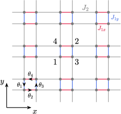
Figure 1: Schematics of the spin analogue of the BBH model described by the Hamiltonian in Eq.(1). Each unit cell contains four sites. Short lines represent intra-cell weak exchange couplings $J_{1x},J_{1y}$, and all units are connected by long lines corresponding to strong couplings $J_{2}$. The left-bottom plaquette exhibits the twist parameters for the $\mathbb{Z}_{4}$ Berry phase.

We consider the following dimerized spin Hamiltonian on a square lattice with four spin-$1/2$ degrees of freedom per unit cell,

$$\hat{H}_{0}=\sum_{{\bf r}} [ J_{1,x}(\hat{h}_{{\bf r},1;{\bf r},3}+\hat{h}_{{\bf r},2;{\bf r},4})$$

$$+ J_{1,y}(\hat{h}_{{\bf r},1;{\bf r},4}+\hat{h}_{{\bf r},2;{\bf r},3})$$

$$+ J_{2,x}(\hat{h}_{{\bf r},3;{\bf r}+\hat{x},1}+\hat{h}_{{\bf r},2;{\bf r}+\hat{x},4})$$

$$+ J_{2,y}(\hat{h}_{{\bf r},4;{\bf r}+\hat{y},1}+\hat{h}_{{\bf r},2;{\bf r}+\hat{y},3})]$$

where $\hat{h}_{{\bf r},i;{\bf r^{\prime}},j}=[S^{x}_{{\bf r},i}S^{x}_{{\bf r^{\prime}},j}+S^{y}_{{\bf r},i}S^{y}_{{\bf r^{\prime}},j}+\Delta S^{z}_{{\bf r},i}S^{z}_{{\bf r^{\prime}},j}]$ with $i,j=1,2,3,4$ marking the site in the unit cell, and $\Delta$ a dimensionless parameter characterizing the anisotropy of the exchange couplings. $S^{\gamma}_{{\bf r},i}$ is spin-$1/2$ operator on the site $i$ of the unit cell at ${\bf r}$, which obeys commutation relations, $\left[S^{\alpha}_{{\bf r},i},S^{\beta}_{{\bf r},j}\right]=i\hbar\varepsilon_{\alpha\beta\gamma}S^{\gamma}_{{\bf r},i}\delta_{ij}\delta_{{\bf r},{\bf r^{\prime}}}$ with $\varepsilon_{\alpha\beta\gamma}$ the Levi-Civita symbol and $\alpha,\beta,\gamma=x,y,z$ representing spin direction. $J_{1,x},J_{1,y}(J_{2,x},J_{2,y})$ are intra(inter)-cell exchange antiferromagnetic (AF) couplings. The model with $\Delta=0(1)$ corresponds to a dimerized XY(Heisenberg) spin system. By tuning the anisotropy $\Delta$, the topological property of the XXZ spin model can also be explored. Throughout the manuscript, we set $J_{2,x}=J_{2,y}=J_{2}=1$ as the energy scale.

In the following discussions, we employ the approach of stochastic series expansion (SSE) QMC method Syljuåsen and Sandvik (2002); Syljuåsen (2003) with directed loop updates to study the model in Eq.(1). The SSE method expands the partition function in power series and the trace is written as a sum of diagonal matrix elements. The directed loop updates make the simulation very efficient et al. (2011); Alet et al. (2005); Pollet et al. (2004). Our simulations are on square lattices with the total number of sites $N=4L\times L$ with $L$ the linear size. There are no approximations causing systematic errors, and the discrete configuration space can be sampled without floating point operations. The temperature is set to be low enough to obtain the ground-state properties. For such spin systems on bipartite lattice, the notorious sign problem in the QMC approach can be avoided.

III The linear spin wave theory

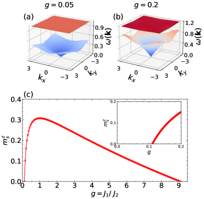
Figure 2: The magnon spectrums at (a) $J_{1}/J_{2}=0.05$ and (b) $J_{1}/J_{2}=0.2$, corresponding to the cases without and with long-range AF orders, respectively. (c) The AF order parameter from the LSWT analysis, Eq. (8). Within LSWT, long-range AF order appears above $g_{c}=0.11$. Here the results are based on the Heisenberg model with $\Delta=1$.

Let us first get some insights on the properties of the model Eq. (1) by LSWT analysis. The Heisenberg model with $\Delta=1$ described by Eq.(1) can be treated within LSWT by replacing the spin operators by bosonic ones via Holstein-Primakoff (HP) transformationHolstein and Primakoff (1940). The transformation on sublattice $1,2$ (the spin is in the positive $z$-direction) is defined as

$$S^{+}_{1(2),i} =a_{i,1(2)},S^{-}_{1(2),i}=a^{\dagger}_{i,1(2)},$$ (2)

$$S^{z}_{1(2),i} =\frac{1}{2}-a^{\dagger}_{i,1(2)}a_{i,1(2)}.$$

On sublattice $3,4$ (the spin is in the negative $z$-direction), the spin operators are defined as

$$S^{+}_{3(4),i} =b^{\dagger}_{i,3(4)},S^{-}_{3(4),i}=b_{i,3(4)},$$ (3)

$$S^{z}_{3(4),i} =b^{\dagger}_{i,3(4)}b_{i,3(4)}-\frac{1}{2}.$$

Then the bosonic tight binding Hamiltonian becomes $H=\sum_{\bf k}X^{\dagger}_{\bf k}{\cal{H}}({\bf k})X_{\bf k}$, where $X_{\bf k}=\left(a_{1\mathit{\mathbf{k}}}^{\dagger}\;\;a_{2\mathit{\mathbf{k}}}^{\dagger}\;\;b_{3\mathit{\mathbf{k}}}\;\;b_{4\mathit{\mathbf{k}}}\;\right)^{T}$ is the basis, and

$$\cal{H}({\bf k})=\left[\begin{array}[]{cccc}C_{0}&0&\gamma_{1\mathit{\mathbf{k}}}&\gamma_{2\mathit{\mathbf{k}}}\\ 0&C_{0}&\gamma_{2\mathit{\mathbf{k}}}^{*}&\gamma_{1\mathit{\mathbf{k}}}^{*}\\ \gamma^{*}_{1\mathit{\mathbf{k}}}&\gamma_{2\mathit{\mathbf{k}}}&C_{0}&0\\ \gamma_{2\mathit{\mathbf{k}}}^{*}&\gamma_{1\mathit{\mathbf{k}}}&0&C_{0}\end{array}\right],$$ (4)

with

$$C_{0} =\frac{1}{2}\left(J_{1x}+J_{1y}\right)+J_{2}$$

$$\gamma_{1\mathit{\mathbf{k}}} =\frac{1}{2}\left(J_{1y}+J_{2}e^{-\textrm{i}k_{y}}\right)$$

$$\gamma_{2\mathit{\mathbf{k}}} =\frac{1}{2}\left(J_{1x}+J_{2}e^{-\textrm{i}k_{x}}\right)$$

The Hamiltonian ${\cal H}({\bf k})$ in Eq.(4) can be diagnalized using Bogliubov transformationToth and Lake (2015). The spin wave spectrum contains two branches, each of which is two-fold degenerate (see Appendix A for the analytical form). The lower energy spin-wave excitations in our model display a linear spectum for small $k$, which is consistent with their AFM nature. For the $C_{4}$ symmetric case, we let $J_{1x}=J_{1y}=J_{1}$, and define the ratio $g=J_{1}/J_{2}$. The magnon spectrums at $g=0.05,0.2$ are shown in Fig.2(a) and (b). Although the spectrums are gapless, there is a gap between the two branches, and its size monotonously decreases as $J_{1}$ is strengthened. The gap vanishes at $J_{1}=J_{2}$ when the system becomes 2D AF Heisenberg model. The resulting gapless spectrum with two branches is connected to the normal one under a two-site unit cell by a folding of the Brillouin zone.

The AFM staggered order parameter defined as

$$m_{s}^{z}=\frac{1}{N}\left(\sum_{i\in(1,2)}\left\langle S_{i}^{z}\right\rangle-\sum_{i\in(3,4)}\left\langle S_{i}^{z}\right\rangle\right)$$ (5)

is obtained in LSWT, where $i\in(1,2)$ denotes those sites which are spin up sublattice sites, and $i\in(3,4)$ denotes those sites which are spin down sublattice sites. Writing $\left\langle S_{i}^{z}\right\rangle$ in terms of HP operators, we have

$$m^{z}_{s} =\frac{1}{N}\left(\sum_{i\in(1,2)}\left\langle S-a_{i}^{\dagger}a_{i}\right\rangle-\sum_{i\in(3,4)}\left\langle b_{i}^{\dagger}b_{i}-S\right\rangle\right)$$

$$= S+\frac{1}{2}-\frac{1}{N}\left(\sum_{{\bf k}}\sum_{i=1}^{4}\left\langle a_{i{{\bf k}}}^{\dagger}a_{i{{\bf k}}}\right\rangle\right),$$

where $S$ is the spin.

We then use the Bogliubov transformation to write the basis $X$ in terms of the diagonal basis $Y=\left(\alpha_{1\mathit{\mathbf{k}}}\;\;\alpha_{2\mathit{\mathbf{k}}}\;\;\beta_{3\mathit{\mathbf{k}}}^{\dagger}\;\;\beta_{4\mathit{\mathbf{k}}}^{\dagger}\;\right)^{T}$: $X=BY$. The Bogliubov transformation matrix $B$ satisfies $Bs_{z}B^{\dagger}=s_{z}$, with

$$s_{z}=\left[\begin{array}[]{cccc}1&0&0&0\\ 0&1&0&0\\ 0&0&-1&0\\ 0&0&0&-1\end{array}\right].$$ (7)

At zero temperature, only the terms containing $\left\langle\beta_{3\mathit{\mathbf{k}}}\beta_{3\mathit{\mathbf{k}}}^{\dagger}\right\rangle=\left\langle\beta_{4\mathit{\mathbf{k}}}\beta_{4\mathit{\mathbf{k}}}^{\dagger}\right\rangle$ are nonzero $(=1)$. Hence the staggered order parameter is

$$m_{s}^{z}=1-\frac{1}{N}\sum_{\mathbf{k}}((B^{\dagger}B)_{33}+(B^{\dagger}B)_{44})$$ (8)

where $(B^{\dagger}B)_{ii}$ denotes the $i$-th element of the matrix $B^{\dagger}B$. Figure 2(c) shows $m_{s}^{z}$ in Eq.(8) as a function of $g$. LSWT greatly underestimates the transition point, and it predicts the Néel-VBS transition at $g_{c}=0.11$. The periodic lattice in Fig.1 is invariant under interchanging $J_{1}$ and $J_{2}$ due to the translation symmetry, indicating a duality between $g$ and $1/g$. Hence there is also a critical value in the large $g$ region, which is exactly $1/g_{c}$ with $g_{c}$ the small critical value. Although the gap size is not affected by the duality, the topological property of the VBS phase changes to be trivial when $J_{1}$ becomes stronger.

IV QMC simulations of the bulk properties

In this section, we investigate the bulk propertires of the higher-order topological spin models using QMC simulations. The properties of the system are controlled by the ratio $J_{1x}/J_{2}$ and $J_{1y}/J_{2}$, and there exist several scenarios. To obtain some insights, let us first discuss two special limits $J_{1x}=J_{1y}=1$ and $J_{1x}=J_{1y}=0$, at which the solutions are well known or exactly solvable. In the former limit, the Hamiltonian Eq. (1) is the XXZ spin model. The case with $\Delta=1$ corresponds to an isotropic AF Heisenberg model, which has a ground state with long-range AF order. In the latter limit, the lattice is decoupled into isolated $2\times 2$ plaquettes. The ground-state energy is $E_{0}=-J_{2}(\Delta+\sqrt{\Delta^{2}+8})/2$, which is separated from the first-excited state by a gap with the size $-J_{2}-E_{0}$ (see Appendix B). While the ground state is in the total $S_{z}=0$ sector, the first-excited state has $S_{z}=\pm 1$. Hence the low-energy excitation is a spin one, which is gapped in the four-site spin chain.

For general cases $J_{1x}\neq 0$ as well as $J_{1y}\neq 0$, a Néel-VBS quantum phase transition can happen by tuning the coupling ratio $J_{1x}/J_{2}$ or $J_{1y}/J_{2}$. The phase transition points can be precisely determined using the SSE QMC by measuring the staggered magnetization $m_{s}^{z}$, the spin stiffness $\rho_{s}$, and the uniform susceptibility $\chi$. Here, the staggered magnetization $m_{s}^{z}$ is defined asWenzel et al. (2008); Sandvik (2010); Ma et al. (2018); Ran et al. (2019); Jiang (2012)

$$m_{s}^{z}=\frac{1}{N}\sum_{i}^{N}S_{i}^{z}(-1)^{x_{i}+y_{i}},$$ (9)

and its Binder ratio is $Q_{2}=\frac{\langle(m_{s}^{z})^{4}\rangle}{\langle(m_{s}^{z})^{2}\rangle^{2}}$Binder (1981); Binder and Landau (1984). The uniform susceptibility writes asWenzel et al. (2008); Sandvik (2010); Ma et al. (2018); Ran et al. (2019)

$$\chi=\frac{\beta}{N}\langle(\sum_{i}^{N}S_{i}^{z})^{2}\rangle.$$ (10)

In terms of SSE configurations, the spin stiffness can be obtained by the expressionWenzel et al. (2008); Sandvik (2010); Ma et al. (2018); Ran et al. (2019)

$$\rho_{s}=\frac{3}{2\beta}(W_{x}^{2}+W_{y}^{2}),$$ (11)

where $W_{\alpha}=(N_{\alpha}^{+}-N_{\alpha}^{-})/L_{\alpha}$ is the winding number in the $\alpha$ ($x$ or $y$) direction, which takes integer values, and represents the times of spin transporting across the system; $N_{\alpha}^{+}(N_{\alpha}^{-})$ denotes the total number of operators transporting spin in the positive (negative) directionnad . Due to the Lorentz symmetry, the correlation length is the same in the space and time directions, and hence the dynamic exponent is $z=1$Troyer et al. (1997). The temperature appears in the argument $L^{z}/\beta$ of the scaling function, thus we took $\beta=L$ to exclude the temperature dependence in the finite-size scaling. At the quantum critical point, the dimensionless quantities $Q_{2},L\chi,L\rho_{s}$ are size-independent, and should cross for different lattice sizes, from which we can extract the phase transition points without knowing the critical exponents.

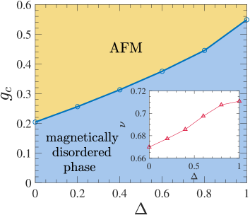
Figure 3: Phase diagram in the $(\Delta,g_{c})$ plane for the $C_{4}$ symmetric ($J_{1x}=J_{1y}$) Hamiltonian in Eq.(1). Inset shows the correlation length critical exponent $\nu$ estimated from the best data collapse of the dimensionless quantities $Q_{2},L\chi,L\rho_{s}$. Here the magnetically disordered phase is a VBSvbs .

Let us first consider the special case with $C_{4}$ symmetry, i.e., $J_{1x}=J_{1y}$ (the value is denoted as $J_{1}$). Figure 3 shows the critical point $g_{c}$ as a function of the anisotropy $\Delta$. For $g<g_{c}$, the system is in the VBS phase, characterized by $m_{s}^{z}=\rho_{s}=\chi=0$. The AF long-range order develops above $g_{c}$, where the values of the staggered magnetization, the spin stiffness and the uniform susceptibility become finite. Since the Néel-VBS phase transition is continuous, $g_{c}$ is determined by the crossings of the above dimensionless quantities. As examples, we show $L\rho_{s}$ at $\Delta=0,1$ for different lattice sizes in Fig.4. Using the leading scaling ansatz for a second-order phase transition,

$$L\rho_{s}=f[(g-g_{c})L^{1/\nu}],$$ (12)

the correlation length critical exponent $\nu$ is determined by the best data collapse. As shown in the inset of Fig.3, $\nu$ increases continuously with $\Delta$. The Heisenberg model with $\Delta=1$ belongs to the three-dimensional (3D) O(3) universality, and the obtained value of $\nu$ is consistent with the standard O(3) one of $\nu=0.7112(5)$Campostrini et al. (2002); Pelissetto and Vicari (2002) For the XY model with $\Delta=0$, the universality class is the 3D XY one. The critical exponent we obtain is $\nu=0.671$, consistent with the accurate results in the literaturePelissetto and Vicari (2002).

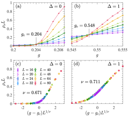
Figure 4: $L\rho_{s}$ as a function of $g=J_{1}/J_{2}$ for the $C_{4}$ symmetric Hamiltonian: (a) $\Delta=0$; (b) $\Delta=1$. The universal crossings determine the transition points $g_{c}=0.204$ in (a) and $g_{c}=0.548$ in (b). (c) and (d) are the corresponding best scaling collapses of $L\rho_{s}$, giving the correlation length critical exponent $\nu=0.671$ for $\Delta=0$ and $\nu=0.711$ for $\Delta=1$, respectively. In all figures, the same lattice sizes are used, and the symbol-size correspondences are shown in (c).

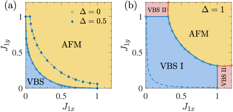
Figure 5: Phase diagrams in the $(J_{1x},J_{1y})$ plane for the model in Eq.(1) with (a) $\Delta=0,0.5$; (b) $\Delta=1$. Dashed lines in (b) indicate the phase boundaries from LSWT. The VBS in (a) and VBS I in (b) are SHOTPs, which have bulk gapped spin excitations, and gapless spin corner states on open lattice. Here VBS I and VBS II are defined relatively to the boundary of the geometry in Fig.1.

Next we map out the phase diagram for general cases in the $(J_{1x},J_{1y})$ plane. Here we only focus on the Heisenberg and XY exchange couplings, and the phase diagrams for $0<\Delta<1$ are similar. The critical points are determined more precisely using the best data collapses with the accurate $\nu$ for the O(3) and XY universality classes. The phase diagrams in Fig. 5 consist of the AFM and VBS phases. The region of VBS shrinks as $\Delta$ is decreased. In both figures, the VBS phases with $J_{1x(y)}/J_{2}<1$ are SHOTPs, which will be demonstrated in the following section. Here the SHOTPs survive only in part of the unit square. In contrast, the electronic HOTIs of the BBH model are in the entire square region $|t_{1x(y)}/t_{2}|<1$ [ $t_{1x(y)}(t_{2})$ denotes the hopping amplitude of the weak (strong) bonds].

Then we consider another limit $J_{1x}=0$ or $J_{1y}=0$, at which the system becomes one-dimensional dimerized spin chain on the boundaries. Under the Jordan-Wigner transformationColeman (2015)

$$S_{i,1}^{+} =\alpha_{i}^{\dagger}\cdot e^{i\pi\sum_{j<i}\left(n_{i,\alpha}+n_{i,\beta}\right)}$$ (13)

$$S_{i,2}^{+} =\beta_{i}^{\dagger}\cdot e^{i\pi\sum_{j<i}\left(n_{j,\alpha}+n_{j,\beta}\right)}e^{i\pi n_{i,\alpha}},$$

$$S^{z}_{i,1(2)} =n_{i,\alpha(\beta)}-1/2$$

the following 1D fermionic Hamiltonian is obtained,

$$H_{f}=\sum_{i}[ \frac{1}{2}(J_{1x(y)}\alpha_{i}^{\dagger}\beta_{i}+J_{2}\beta^{\dagger}_{i}\alpha_{i+1}+\textrm{H.c.})+$$ (14)

$$J_{1x(y)}\Delta(n_{i,\alpha}-\frac{1}{2})(n_{i,\beta}-\frac{1}{2})+$$

$$J_{2}\Delta(n_{i,\beta}-\frac{1}{2})(n_{i+1,\alpha}-\frac{1}{2})],$$

where $\alpha_{i},\beta_{i}$ are annihilation operators of spinless fermions on the two sites of unit cell $i$, and $n_{i,\alpha}=\alpha^{\dagger}_{i}\alpha_{i},n_{i,\beta}=\beta^{\dagger}_{i}\beta_{i}$ are the corresponding number operators. In the hopping term connecting the boundary, there is an additional phase $e^{i\pi n_{t}}$ ($n_{t}$ the total number of fermions), which may be $1$ or $-1$ depending on even or odd $n_{t}$. Since such a sign has no effect on the 1D boundary mode, it does not affect the topological property of the system, and we omit it in the above Hamiltonian. For the XY model, the mapped fermionic Hamiltonian is the noninteracting Su-Schrieffer-Heeger (SSH) modelSu et al. (1979), which has a topological phase transition at $J_{1x(y)}=J_{2}$. The 1D dimerized Heisenberg model corresponds to an interacting SSH model with dimerized nearest-neighbor repulsions. It has been shown that an AFM transition occurs at $J_{1x(y)}=J_{2}$Cazalilla et al. (2011); Mishra et al. (2011). We calculate the 1D topological invariant, i.e., the Zak phase, which is $\gamma=1$ for $J_{1x(y)}<J_{2}$ and $\gamma=0$ for $J_{1x(y)}>J_{2}$ (see Appendix C). This unambiguously shows the topological phase transition happens exactly at the uniform point, which determines the on-axis points of the phase boundary in Fig.5.

It is noted that the transition line between VBS I and VBS II is a straight line. In this region, the dimensionless quantities, such as $L\rho_{s}$ $L\chi$, do not exhibit universal crossings as $J_{1x}(J_{1y})$ varies at fixed $J_{1y}(J_{1x})$, and instead their values continuously decrease with increasing $L$. These imply the absence of a Néel-VBS transition, and the system keeps in the VBS phase. Since there is a duality between $J_{1x(y)}<1$ and $J_{1x(y)}>1$, the transition point should be exactly at $J_{1x(y)}^{c}=1$. Otherwise it will generate a contradictory result. Let us explain this point more clear. Suppose $J_{1x}^{c}<1$ for fixed $J_{1y}$ in the straight-line region. Then there are two topological transition points due to the duality, and an intermediate phase exists in the region $J_{1x}^{c}<J_{1x}<1/J_{1x}^{c}$. Since the VBS with $J_{1x}<J_{1x}^{c}(J_{1x}>1/J_{1x}^{c})$ is adiabatically connected to the $J_{1x}=0(J_{1x}=\infty)$ topologically nontrivial (trivial) phase, the intermediate phase has contradictory topological properties from the topological transitions of the two different sides, suggesting it should not exist in real system and the transition point is exactly at $J_{1x}^{c}=1$.

In the following sections, we will show that the VBS for $J_{1x}<1$ or $J_{1y}<1$, which is denoted as VBS I, has nontrivial higher-order topological property, while the other one (denoted as VBS II) is topologically trivial.

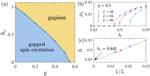
Figure 6: (a) Phase diagram in the $(g,h_{c})$ plane for the Hamiltonian $\hat{H_{0}}+\hat{H_{1}}$ with $\Delta=1$. Below $h_{c}$, the system remains in the VBS phase with gapped spin excitation. However the spins are aligned along the direction of the applied magnetic field above $h_{c}$, displaying ferromagnetic behavior. (b) $\rho_{s}$ vs $h$ near the transition point at $g=0.1$ for several lattice sizes. The data are fitted using the functional form $\rho_{s}\sim[h-h_{c}(L)]^{\frac{1}{2}}$ (solid lines). (c) $h_{c}$ at $g=0.1$ obtained by extrapolating $h_{c}(L)$ to the thermodynamic limit. Here we consider the $C_{4}$-symmetric case with $g=J_{1}/J_{2}$ and $J_{2}=1$.

In the above phase diagrams, the VBS phases are gapped in the spin excitation while the AF state is gapless. To see this explicitly, we add a magnetic field perpendicular to the lattice described by

$$\hat{H}_{1}=-\sum_{{\bf r}}\sum_{i=1}^{4}hS^{z}_{{\bf r},i}.$$ (15)

The total Hamiltonian $\hat{H}_{0}+\hat{H}_{1}$ is then simulated by the QMC method. The magnetization density

$$m_{z}=\frac{1}{N}\sum_{i}^{N}S_{i}^{z},$$ (16)

is further measured. We find $m_{z}$ and $\rho_{s}$ remain to be zero up to a finite magnetic field. Afterwards, they continuously increase, and the system is in a ferromagnetic phase. To determine the transition values precisely, we fit the data with $\rho_{s}\sim[h-h_{c}(L)]^{\beta}$ around the critical point for each lattice sizeKrzakala et al. (2008); Capogrosso-Sansone et al. (2008). As shown in Fig.6(b), our data are compatible with the mean-field exponent $\beta=\frac{1}{2}$. Then $h_{c}$ is obtained by extrapolating $h_{c}(L)$ to the thermodynamic limit [see Fig.6(c)]. By this way, the phase diagram in the $(g,h_{c})$ plane is plotted in Fig.6(a). Below $h_{c}$, the system remains in the VBS phase with gapped spin excitations. However the spins are aligned along the direction of the applied magnetic field above $h_{c}$, displaying a ferromagnetic behavior with gapless spin excitations. The critical value is exactly $h_{c}=1$ at $g=0$, when the system is decoupled into isolated plaquettes, and can be understood analytically. The spin dimer can be in a spin-singlet ( or spin-triplet) state, with the energy $-\frac{3}{4}J_{2}$ (or $\frac{1}{4}J_{2}-h$). So the transition point is $h=J_{2}=1$, after which the ground state becomes the spin-triplet one where the spins are aligned to the same direction by the magnetic field.

It is interesting to note that the spin-gapped VBS phases are higher-order topological spin states. Next we will demonstrate that gapless spin corner modes will appear on open lattices in both $x$- and $y$-directions due to nontrivial higher-order bulk topology.

V the spin corner modes

In this section, we demonstrate the spin corner modes, which consists of the characteristic signatures of nontrivial SHOTPs. Here we consider a square geometry with open boundary condition, which preserves the mirror symmetry $M_{x},M_{y}$, the inversion symmetry, and the rotation symmetry $C_{2}$. For other geometries, a general principle is that a corner state will appear as long as a domain wall is formed by the two edges crossing at the corner. The SHOTP within $J_{1x(y)}/J_{2}<1$ is adiabatically connected to the limit $J_{1x(y)}=0$, where there are four dangling spins at the corners. For finite $J_{1x(y)}$, the gapless spin corner modes should remain on open lattices in the SHOTP. A infinitesimal magnetic field $h$ can align these corner spins, thus the total magnetization becomes $M_{z}=Nm_{z}=2$, compared to $M_{z}=0$ in the bulk SHOTP. Besides, the magnetization is mainly localized near the corners, and the localization length increases with increasing $J_{1x(y)}$ due to the decreasing of the spin gap. Figure 7 shows the total magnetization as a function of $h$ at $J_{1}/J_{2}=0.1$ (the $C_{4}$ symmetric case) on a $L=40$ open lattice. It is noted that the origin of the $M_{z}=2$ plateau tends to be zero as $\beta$ is increased, implying the plateau is quantized as long as $h$ becomes nonzero in the limit of zero temperature. Beside, the $M_{z}=2$ plateau persists to a finite $h$, and only begins to vanish when the spin gap closes. We also show the local distribution of the magnetization for $J_{1}/J_{2}=0.1$ in Fig.7(b). Indeed the magnetization is localized near the corners, implying the gapless corner spins leads to the quantized magnetization.

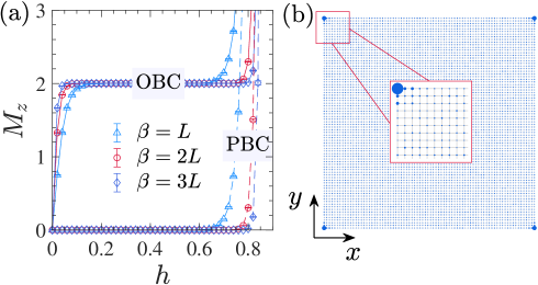
Figure 7: (a) The total magnetization as a function of $h$ under open and periodic boundary conditions at different inverse temperatures. The origin of the $M_{z}=2$ plateau tends to be zero in the limit $\beta\rightarrow\infty(T=0)$. (b) Local distribution of $M_{z}$ induced by a magnetic field $h=0.2$ on a $L=40$ open lattice. Four spins are localized around the corners, giving rise to the quantized magnetization $M_{z}=2$.

Such results are also valid for larger $J_{1}/J_{2}$ as long as the ratio is less than the critical value $g_{c}=0.548$ (see Appendix D). Since the appearance of the spin corner states is a manifestation of the nontrivial higher-order topological property, the Néel-VBS transition is also a higher-order topological phase transition. Besides, we perform the calculations of $M_{z}-h$ curves with very small steps near the straight-line boundary of the phase diagram in Fig.5(b). The $M_{z}$ plateau characterizing the spin corner states immediately vanishes as $J_{1x}$ crosses the boundary located at $J^{c}_{1x}=1$, thus verifies the straight phase boundary with very high accuracy (see Appendix D).

VI The higher-order topological invariant

The appearance of gapless spin corner states is due to the bulk higher-order topological protection, and the bulk topology is generally characterized by a topological invariant. A $\mathbb{Z}_{4}$ Berry phase is proposed as the topological invariant for the $C_{4}$-symmetric SHOTP. It is defined with respect to the local twist of the Hamiltonian, which is parameterized by three independent variables $\Theta=(\theta_{1},\theta_{2},\theta_{3})$ ranged in $[0,2\pi)$Araki et al. (2020). The Hamiltonian is decomposed into two types of plaquettes with weak and strong bonds, respectively. The twist parameters are introduced to the spin operators on any one of the plaquettes as: $\tilde{S}^{+}_{i}=e^{-i\varphi_{i}}S^{+}_{i},\tilde{S}^{-}_{i}=e^{i\varphi_{i}}S^{-}_{i}$, with $\varphi_{i}=\sum_{q=1}^{i}\theta_{i}$ for $i=1,2,3,4$ and $\varphi_{4}=0$. The $\mathbb{Z}_{4}$ Berry phase is defined as

$$\gamma_{z_{4}}=i\oint_{L_{j}}\left\langle\Psi_{\Theta}\left|\frac{d}{d\Theta}\right|\Psi_{\Theta}\right\rangle$$ (17)

where the path $L_{j}(j=1,2,3,4)$ is in the parameter space: $E_{j-1}\rightarrow G\rightarrow E_{j}$ with $E_{1}=(2\pi,0,0),E_{2}=(0,2\pi,0),E_{3}=(0,0,2\pi),E_{0}=E_{4}=(0,0,0)$, and $G=1/4\sum_{j=1}^{4}E_{j}$, and $\Psi_{\Theta}$ is the corresponding groundstate many-body wave function at half-filling. In our calculations, we choose the left-bottom plaquette to apply the local twist (see Fig.1). Figure 8 shows the $\mathbb{Z}_{4}$ Berry phase in the $(g,\Delta)$ plane. As $g$ increases at fixed $\Delta$, the value of the $\mathbb{Z}_{4}$ Berry phase changes abruptly from $\pi$ to $0$ at a critical $g_{c}$, marking a topological phase transition. The critical values are $g_{c}(\Delta=1)=1$ and $g_{c}(\Delta=1)=1.19$, respectively. For intermediate $\Delta$, the critical value continuously decreases with increasing $\Delta$. Compared to the QMC results, the $\mathbb{Z}_{4}$ Berry phase greatly overestimates the transition point, and the quantized value persists in the AF phase, which has also been found in other works, and has been attributed to the finite-size errorBibo et al. (2020). Since the Néel-VBS transition is continuous, the two phases coexist near the transition point on small finite lattices. Besides, a finite-size gap exists even in the AF phase. Hence although the $\mathbb{Z}_{4}$ Berry phase is quantized, it still fails to determine the phase boundary precisely. Another method of calculating the topological invariant in terms of the many-body quadrupole momentum also suffers significant finite-size errorsWheeler et al. (2019); Kang et al. (2019) (see Appendix E), and identifying a solid many-body topological invariant requires further studiesYou et al. (2020).

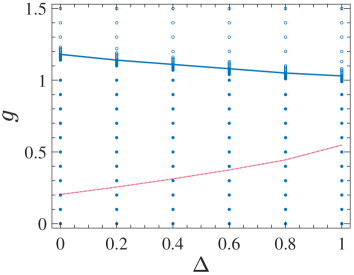
Figure 8: The $\mathbb{Z}_{4}$ Berry phase in the $(g,\Delta)$ plane, where the filled (open) blue circle at each parameter set represent nontrivial value $\pi$ (trivial value $0$). The solid blue line is the phase boundary determined by the $\mathbb{Z}_{4}$ Berry phase. The QMC result (dotted red line) is also plotted for comparison.

VII Connection to the BBH-Hubbard model

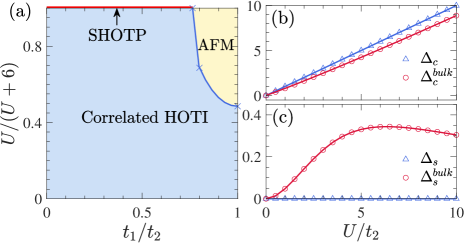
Figure 9: (a) Phase diagram of the fermionic BBH-Hubbard model. The $U=\infty$ Heisenberg limit is along the top of the figure, $U/(6+U)=1$, and is extracted from the data of Fig. 3. $U_{c}$ at $t_{1}/t_{2}=0.8,1$ are from Refs.Otsuka et al. (2016); Peng et al. (2020). Charge (b) and spin (c) excitation gaps in the limit $t_{1}=0$ under periodic and open boundary conditions.

Here we further compare SHTOPs discussed in previous sections with correlated HOTIs for a better understanding of their properties. The Heisenberg model with $\Delta=1$ in Eq.(1) is the large-$U$ limit of the BBH electronic model subjected to an on-site Hubbard interaction $H_{U}=U\sum_{i}n_{i\uparrow}n_{i\downarrow}$, with $n_{i\sigma}=c^{\dagger}_{i\sigma}c_{i\sigma}$ and $c^{\dagger}_{i\sigma},c_{i\sigma}$ the electronic creation and annihilation operators with spin $\sigma=\uparrow,\downarrow$. At $t_{1}/t_{2}=1$, the BBH model becomes the $\pi$-flux lattice hosting 2D Dirac fermionsWang et al. (2014); Li et al. (2015); Parisen Toldin et al. (2015); Otsuka et al. (2016); Guo et al. (2018). The Hubbard interaction drives a semimetal-AFM quantum phase transition, with the most accurate value of the critical point $U_{c}=5.65\pm 0.05$Parisen Toldin et al. (2015); Otsuka et al. (2016). In the large-$U$ limit, the relation $J=4t^{2}/U$ gives the exchange constant in terms of $U$ and the hopping amplitude. Since the VBS-AFM transition happens at $g_{c}=0.584$, there is a critical ratio for $t_{1}/t_{2}$ at $f_{c}=\sqrt{g_{c}}=0.764$. Below $f_{c}$, the correlated HOTI continuously evolves into the SHOTP as $U$ increases, and meanwhile the spin excitation remains gapped in the bulk systems. However above the critical point $f_{c}$, there is a AFM transition, from which the bulk spin excitation becomes gapless, and hence the correlated HOTI vanishes. The above discussion is summarized as the phase diagram in the $(t_{1}/t_{2},U)$ plane, shown in Fig.9(a).

In the correlated HOTI, the spin excitation is gapless, but the charge excitation is gapped on open lattices. Figure 9(b) and (c) shows these gaps as a function of $U$ in the limit $t_{1}=0$. At half filling, each of the four isolated corner sites is occupied by one electron. Adding an opposite spin electron to any such site unavoidably induces the interacting energy $U$, and thus the charge excitation gap is $\Delta_{c}=U$. However the spin excitation by flipping the corner spin does not cost any energy, and the spin excitation gap is $\Delta_{s}=0$. We also calculated these gaps in the bulk system, which are defined as follows: $\Delta^{bulk}_{c}=(E_{N+1,S_{z}=1/2}+E_{N-1,S_{z}=-1/2}-2E_{N,S_{z}=0})/2$, and $\Delta^{bulk}_{s}=(E_{N,S_{z}=1}+E_{N,S_{z}=-1}-2E_{N,S_{z}=0})/2$, where $E_{N,S_{z}}$ is the ground-state energy with the total number of electrons $N$ and the total spin in the $z$-direction $S_{z}$. As shown in Fig.9(b) and (c), both of them are gapped. So the correlated HOTIs have similar bulk-boundary correspondence as the spin counterparts, i.e., the appearance of gapless spin corner states protected by the higher-order topology.

VIII Conclusions

In summary, we investigate the higher-order topological properties of spin analogues of the BBH model using large-scale QMC simulations. Generally two spin quantum phases, i.e., VBS and AFM, may appear in the system. A continuous phase transition can be driven by tuning the ratio between the weak and strong couplings. We identify the VBS phase with $J_{1x(y)}/J_{2}<1$ to be a nontrivial SHOTP, which is characterized by a bulk spin excitation gap and gapless spin corner states on open lattice. Besides, in the large-$U$ limit, the SHOTP is continuously connected to the electronic correlated HOTI in the BBH-Hubbard model. They share the same bulk-boundary correspondence: the appearance of gapless corner spin excitations protected by nontrivial higher-order topology. The SHOTPs also exist in XXZ spin models, but their regions in the phase diagrams shrink as the anisotropy $\Delta$ decreases. Our results explicitly demonstrate the higher-order topological properties of spin systems, and contribute to further understandings of the many-body higher-order topological phenomena.

Appendix A The analytical form for the spin wave spectrum of the Hamiltonian in Eq.(4)

The spin wave spectrum of the Hamiltonian in Eq.(4) in the main text can be obtained analytically. The two branches(each of which is two-fold degenerate) are as follows,

$$\omega_{1}(\mathbf{k}) = \sqrt{[C_{3}+D({\bf k})-(C_{1}\cos k_{x}+C_{2}\cos k_{y})]/2},$$

$$\omega_{2}(\mathbf{k}) = \sqrt{[C_{3}-D({\bf k})-(C_{1}\cos k_{x}+C_{2}\cos k_{y})]/2},$$

$$D({\bf k}) = \sqrt{C_{4}+D_{1}({\bf k})+D_{2}({\bf k})},$$

where $D_{1}({\bf k})=C_{5}\cos\left(k_{y}\right)+C_{6}\cos\left(k_{x}\right)$, $D_{2}({\bf k})=4C_{1}C_{2}\cos\left(k_{x}\right)\cos\left(k_{y}\right)$, and

$$C_{1} =J_{1x}J_{2}$$

$$C_{2} =J_{1y}J_{2}$$

$$C_{3} =\left(J_{1x}J_{1y}+J_{2}^{2}+2J_{1x}J_{2}+2J_{1y}J_{2}\right)$$

$$C_{4} =\left(J_{2}^{4}+J_{2}^{2}J_{1x}^{2}+J_{2}^{2}J_{1y}^{2}+J_{1x}^{2}J_{1y}^{2}\right)$$

$$C_{5} =2J_{2}J_{1y}\left(J_{2}^{2}+J_{1x}^{2}\right)$$

$$C_{6} =2J_{2}J_{1x}\left(J_{2}^{2}+J_{1y}^{2}\right).$$

Appendix B The exact solution of the spin Hamiltonian in Eq.(1) on a plaquette

In the limit $J_{1}=0$, the lattice is decoupled into isolated $2\times 2$ plaquettes, on which the spin Hamiltonian in Eq.(1) can be solved by diagonalizing the Hamiltonian matrix. Actually each plaquette is a one-dimensional chain with four sites. For the $S_{z}=0$ sector, there are six basis states: $|\uparrow\uparrow\downarrow\downarrow\rangle,|\uparrow\downarrow\uparrow\downarrow\rangle,|\uparrow\downarrow\downarrow\uparrow\rangle,|\downarrow\uparrow\uparrow\downarrow\rangle,|\downarrow\uparrow\downarrow\uparrow\rangle,|\downarrow\downarrow\uparrow\uparrow\rangle$. Under the above basis, the Hamiltonian matrix writes as

$$H_{S_{z}=0}=J_{2}\left(\begin{array}[]{cccccc}0&\frac{1}{2}&0&0&\frac{1}{2}&0\\ \frac{1}{2}&-\Delta&\frac{1}{2}&\frac{1}{2}&0&\frac{1}{2}\\ 0&\frac{1}{2}&0&0&\frac{1}{2}&0\\ 0&\frac{1}{2}&0&0&\frac{1}{2}&0\\ \frac{1}{2}&0&\frac{1}{2}&\frac{1}{2}&-\Delta&\frac{1}{2}\\ 0&\frac{1}{2}&0&0&\frac{1}{2}&0\\ \end{array}\right).$$ (24)

The lowest two eigenvalues are $-J_{2}(\Delta+\sqrt{\Delta^{2}+8})/2,-J_{2}\Delta$, respectively.

For the $S_{z}=1$ sector, the basis is: $|\uparrow\uparrow\uparrow\downarrow\rangle,|\uparrow\uparrow\downarrow\uparrow\rangle,|\uparrow\downarrow\uparrow\uparrow\rangle,|\downarrow\uparrow\uparrow\uparrow\rangle$, under which the Hamiltonian matrix is,

$$H_{S_{z}=1}=J_{2}\left(\begin{array}[]{cccc}0&\frac{1}{2}&0&\frac{1}{2}\\ \frac{1}{2}&0&\frac{1}{2}&0\\ 0&\frac{1}{2}&0&\frac{1}{2}\\ \frac{1}{2}&0&\frac{1}{2}&0\\ \end{array}\right).$$ (29)

The lowest eigenvalue is $-J_{2}$. The $S_{z}=-1$ sector has exactly the same solution. There is only a diagonal energy for the $S_{z}=\pm 2$ sectors, which is $J_{2}\Delta$.

Sorting all the above eigenvalues, the ground-state energy is $E_{0}=-J_{2}(\Delta+\sqrt{\Delta^{2}+8})/2$ in the $S_{z}=0$ sector, and the first-exited state has $E_{1}=-J_{2}$ in the $S_{z}=\pm 1$ sector. Hence a gap with the size $-J_{2}-E_{0}$ separates the two lowest levels.

Appendix C The Zak phase of the 1D fermionic Hamiltonian in Eq.(14)

We calculate the Zak phase of the ground-state at half-filling using the twisted boundary conditionsGuo and Shen (2011). It is defined as

$$\gamma=\frac{1}{2\pi}\oint i\langle\psi_{\theta}|\frac{d}{d\theta}|\psi_{\theta}\rangle,$$

where $\theta$ is the twisted boundary phase which takes values from $0$ to $2\pi$ and $\psi_{\theta}$ is the corresponding ground-state many-body wave function at half-filling obtained by the exact diagonalization method. The $J_{1y}=0$ limit is considered, and the $J_{1x}=0$ limit is the same. As shown in Fig.10, the gap between the ground- and the first-excited states vanishes at $J_{1x}=1$, and the Zak phase $\gamma$ has the value $1$ and $0$ for $J_{1x}<1$ and $J_{1x}>1$, respectively. These clearly show that critical point of the $J_{1y}=0$ limit is exactly at $J_{1x}=1$, determining the on-axis points of the phase diagram in Fig.5(b).

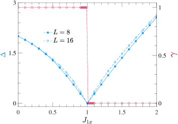
Figure 10: The gap between the ground- and the first-excited states and the Zak phase as a function of $J_{1x}$. The topological phase transition occurs at $J_{1x}=1$, where the gap vanishes, and the Zak phase changes its value from $\pi$ to $0$. Here $J_{2}=1$.

Appendix D More results of the quantized magnetization by the spin corner states

Due to the bulk-boundary correspondence, the spin corner modes will appear on the lattices with open boundary condition (OBC) when the system is in the SHOTP. They can be demonstrated by applying an external magnetic field $h$, and a $M_{z}=2$ plateau, caused by the polarization of the corner spins, exists in the $M_{z}-h$ curve. Figure 11(a) plots $M_{z}$ as a function of $h$ on periodic lattices. $M_{z}$ remains zero up to a finite magnetic field $h_{c}$, which is proportional to the gap size. When the boundary condition becomes open, the characteristic plateau always exists in the gap for $g<g_{c}$ (here $g_{c}=0.548$), but the curves for $g>g_{c}$ are almost unchanged compared to their periodic counterparts. These clearly show that the appearance of the spin corner states are only below the critical point. Hence a topological phase transition happens accompanying the Néel-VBS transition, and the VBS state below $g_{c}$ has nontrivial spin higher-order topological property.

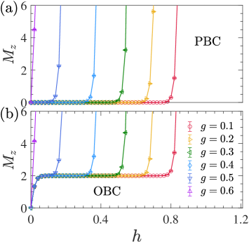
Figure 11: The total magnetization as a function of $h$ at different $g$ under periodic (a) and open (b) boundary conditions. Here the system is $C_{4}$-symmetric with the lattice size $L=40$ and the inverse temperature is $\beta=2L$.

We also perform similar calculations with very small steps near the straight-line boundary of the phase diagram in Fig.5(b). As shown in Fig.12, the $M_{z}$ plateau immediately vanishes as $J_{1x}$ crosses the boundary located at $J^{c}_{1x}=1$, verifying the phase boundary with very high accuracy.

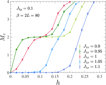
Figure 12: The total magnetization as a function of $h$ at different $J_{1x}$ with fixed $J_{1y}=0.1$ under open boundary condition. The transition point is at $J_{1x}=1$, thus the quantized plateau immediately vanishes as $J_{1x}>1$. Here the lattice size is $L=40$, and the inverse temperature is $\beta=2L$.

Appendix E Another method of calculating the topological invariant

Another method of calculating the topological invariant in terms of the many-body quadrupole moment is formulated as followsWheeler et al. (2019); Kang et al. (2019):

$$q_{xy}=\frac{1}{2\pi}\mathrm{Imlog}\langle\Psi_{G}|\hat{U}_{2}|\Psi_{G}\rangle,$$ (30)

where $|\Psi_{G}\rangle$ is the many-body ground states, and $\hat{U}_{2}\equiv\exp[i2\pi\hat{q}_{xy}]$ with $\hat{q}_{xy}=\sum_{{\bf r}}xy\hat{n}({\bf r})/(L_{x}L_{y})$ as quadrupole moment density operator per unit cell at position ${\bf r}$. Here $L_{x,y}$ are the sizes of the systems along $x$- and $y$- directions. The spin-1/2 operators can be mapped to the hardcore boson representation, where the spin operators are written in terms of hardcore boson creation and annihilation operators

$$S^{\dagger}_{i}=b^{\dagger}_{i},\ S_{i}=b_{i},\ S^{z}_{i}=b^{\dagger}_{i}b_{i}-\frac{1}{2}.$$ (31)

Hence $\hat{n}({\bf r})$ in $\hat{q}_{xy}$ can be understood as the number operator of hardcore bosons.

The definition in Eq.(E1) can be used in the entire parameter space, including the cases with $J_{1x}\neq J_{1y}$. However since the coordinates of each site use those of the unit cell it belongs to and a 16-site geometry has only $2\times 2$ unit cells, this definition has larger finite-size error, and the ED calculations on a 16-site geometry give uncorrect results. We demonstrate the size dependence of this approach based on the noninteracting BBH model. As shown in Fig.13, the result becomes reasonable only for $L\geq 4$, i.e., $N\geq 64$ sites, which can hardly be accessed by the ED method.

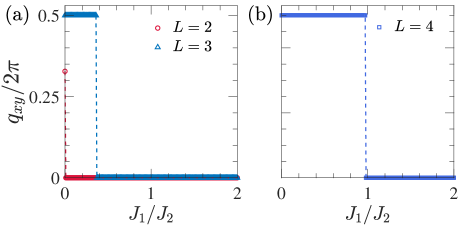
Figure 13: The size dependence of the quadrupole moment based on the noninteractinng BBH model: (a) $L=2,3$; (c) $L=4$. Here we consider the $C_{4}$-symmetric case with the critical point at $J_{1}/J_{2}=1$. The finite-size error only becomes negligible for $L\geq 4$.

References

- Benalcazar et al. (2017a) W. A. Benalcazar, B. A. Bernevig, and T. L. Hughes, Science 357, 61 (2017a), ISSN 0036-8075, URL https://science.sciencemag.org/content/357/6346/61.
- Benalcazar et al. (2017b) W. A. Benalcazar, B. A. Bernevig, and T. L. Hughes, Phys. Rev. B 96, 245115 (2017b), URL https://link.aps.org/doi/10.1103/PhysRevB.96.245115.
- Song et al. (2017) Z. Song, Z. Fang, and C. Fang, Phys. Rev. Lett. 119, 246402 (2017), URL https://link.aps.org/doi/10.1103/PhysRevLett.119.246402.
- Langbehn et al. (2017) J. Langbehn, Y. Peng, L. Trifunovic, F. von Oppen, and P. W. Brouwer, Phys. Rev. Lett. 119, 246401 (2017), URL https://link.aps.org/doi/10.1103/PhysRevLett.119.246401.
- Khalaf (2018) E. Khalaf, Phys. Rev. B 97, 205136 (2018), URL https://link.aps.org/doi/10.1103/PhysRevB.97.205136.
- Schindler et al. (2018a) F. Schindler, A. M. Cook, M. G. Vergniory, Z. Wang, S. S. P. Parkin, B. A. Bernevig, and T. Neupert, Science Advances 4 (2018a).
- Slager et al. (2015) R.-J. Slager, L. Rademaker, J. Zaanen, and L. Balents, Phys. Rev. B 92, 085126 (2015), URL https://link.aps.org/doi/10.1103/PhysRevB.92.085126.
- Călugăru et al. (2019) D. Călugăru, V. Juričić, and B. Roy, Phys. Rev. B 99, 041301 (2019), URL https://link.aps.org/doi/10.1103/PhysRevB.99.041301.
- Ezawa (2018a) M. Ezawa, Phys. Rev. Lett. 120, 026801 (2018a), URL https://link.aps.org/doi/10.1103/PhysRevLett.120.026801.
- Lin and Hughes (2018) M. Lin and T. L. Hughes, Phys. Rev. B 98, 241103 (2018), URL https://link.aps.org/doi/10.1103/PhysRevB.98.241103.
- Yan et al. (2018) Z. Yan, F. Song, and Z. Wang, Phys. Rev. Lett. 121, 096803 (2018), URL https://link.aps.org/doi/10.1103/PhysRevLett.121.096803.
- Wang et al. (2018) Q. Wang, C.-C. Liu, Y.-M. Lu, and F. Zhang, Phys. Rev. Lett. 121, 186801 (2018), URL https://link.aps.org/doi/10.1103/PhysRevLett.121.186801.
- Kunst et al. (2018) F. K. Kunst, E. Edvardsson, J. C. Budich, and E. J. Bergholtz, Phys. Rev. Lett. 121, 026808 (2018), URL https://link.aps.org/doi/10.1103/PhysRevLett.121.026808.
- Liu et al. (2019a) T. Liu, Y.-R. Zhang, Q. Ai, Z. Gong, K. Kawabata, M. Ueda, and F. Nori, Phys. Rev. Lett. 122, 076801 (2019a), URL https://link.aps.org/doi/10.1103/PhysRevLett.122.076801.
- Ghatak and Das (2019) A. Ghatak and T. Das, Journal of Physics: Condensed Matter 31, 263001 (2019), URL https://doi.org/10.1088%2F1361-648x%2Fab11b3.
- Imhof et al. (2018) S. Imhof, C. Berger, F. Bayer, J. Brehm, L. W. Molenkamp, T. Kiessling, F. Schindler, C. H. Lee, M. Greiter, T. Neupert, et al., Nature Physics 14, 925 (2018).
- Serra-Garcia et al. (2019) M. Serra-Garcia, R. Süsstrunk, and S. D. Huber, Phys. Rev. B 99, 020304 (2019), URL https://link.aps.org/doi/10.1103/PhysRevB.99.020304.
- Ezawa (2018b) M. Ezawa, Phys. Rev. B 98, 201402 (2018b), URL https://link.aps.org/doi/10.1103/PhysRevB.98.201402.
- Peterson et al. (2018) C. W. Peterson, W. A. Benalcazar, T. L. Hughes, and G. Bahl, Nature 555, 346 (2018).
- Ma et al. (2019) G. Ma, M. Xiao, and C. T. Chan, Nature Reviews Physics 1, 281 (2019).
- Fan et al. (2019) H. Fan, B. Xia, L. Tong, S. Zheng, and D. Yu, Phys. Rev. Lett. 122, 204301 (2019), URL https://link.aps.org/doi/10.1103/PhysRevLett.122.204301.
- Zilberberg et al. (2018) O. Zilberberg, S. Huang, J. Guglielmon, M. Wang, K. P. Chen, Y. E. Kraus, and M. C. Rechtsman, Nature 553, 59 (2018).
- Noh et al. (2018) J. Noh, W. A. Benalcazar, S. Huang, M. J. Collins, K. P. Chen, T. L. Hughes, and M. C. Rechtsman, Nature Photonics 12, 408 (2018).
- Xue et al. (2019) H. Xue, Y. Yang, F. Gao, Y. Chong, and B. Zhang, Nature materials 18, 108 (2019).
- Ni et al. (2019) X. Ni, M. Weiner, A. Alu, and A. B. Khanikaev, Nature materials 18, 113 (2019).
- Xie et al. (2018) B.-Y. Xie, H.-F. Wang, H.-X. Wang, X.-Y. Zhu, J.-H. Jiang, M.-H. Lu, and Y.-F. Chen, Physical Review B 98, 205147 (2018).
- Zhang et al. (2019) X. Zhang, H.-X. Wang, Z.-K. Lin, Y. Tian, B. Xie, M.-H. Lu, Y.-F. Chen, and J.-H. Jiang, Nature Physics 15, 582 (2019).
- Xie et al. (2019) B.-Y. Xie, G.-X. Su, H.-F. Wang, H. Su, X.-P. Shen, P. Zhan, M.-H. Lu, Z.-L. Wang, and Y.-F. Chen, Phys. Rev. Lett. 122, 233903 (2019), URL https://link.aps.org/doi/10.1103/PhysRevLett.122.233903.
- El Hassan et al. (2019) A. El Hassan, F. K. Kunst, A. Moritz, G. Andler, E. J. Bergholtz, and M. Bourennane, Nature Photonics 13, 697 (2019).
- Chen et al. (2019) X.-D. Chen, W.-M. Deng, F.-L. Shi, F.-L. Zhao, M. Chen, and J.-W. Dong, Phys. Rev. Lett. 122, 233902 (2019), URL https://link.aps.org/doi/10.1103/PhysRevLett.122.233902.
- Mittal et al. (2019) S. Mittal, V. V. Orre, G. Zhu, M. A. Gorlach, A. Poddubny, and M. Hafezi, Nature Photonics 13, 692 (2019).
- Schindler et al. (2018b) F. Schindler, Z. Wang, M. G. Vergniory, A. M. Cook, A. Murani, S. Sengupta, A. Y. Kasumov, R. Deblock, S. Jeon, I. Drozdov, et al., Nature physics 14, 918 (2018b).
- Liu et al. (2019b) B. Liu, G. Zhao, Z. Liu, and Z. F. Wang, Nano Letters 19, 6492 (2019b), URL https://doi.org/10.1021/acs.nanolett.9b02719.
- Sheng et al. (2019) X.-L. Sheng, C. Chen, H. Liu, Z. Chen, Z.-M. Yu, Y. X. Zhao, and S. A. Yang, Phys. Rev. Lett. 123, 256402 (2019), URL https://link.aps.org/doi/10.1103/PhysRevLett.123.256402.
- Chen et al. (2020) C. Chen, Z. Song, J.-Z. Zhao, Z. Chen, Z.-M. Yu, X.-L. Sheng, and S. A. Yang, Phys. Rev. Lett. 125, 056402 (2020), URL https://link.aps.org/doi/10.1103/PhysRevLett.125.056402.
- Peng et al. (2020) C. Peng, R.-Q. He, and Z.-Y. Lu, Phys. Rev. B 102, 045110 (2020), URL https://link.aps.org/doi/10.1103/PhysRevB.102.045110.
- Kudo et al. (2019) K. Kudo, T. Yoshida, and Y. Hatsugai, Phys. Rev. Lett. 123, 196402 (2019), URL https://link.aps.org/doi/10.1103/PhysRevLett.123.196402.
- Bibo et al. (2020) J. Bibo, I. Lovas, Y. You, F. Grusdt, and F. Pollmann, Phys. Rev. B 102, 041126 (2020), URL https://link.aps.org/doi/10.1103/PhysRevB.102.041126.
- Dubinkin and Hughes (2019) O. Dubinkin and T. L. Hughes, Phys. Rev. B 99, 235132 (2019), URL https://link.aps.org/doi/10.1103/PhysRevB.99.235132.
- You et al. (2018) Y. You, T. Devakul, F. J. Burnell, and T. Neupert, Phys. Rev. B 98, 235102 (2018), URL https://link.aps.org/doi/10.1103/PhysRevB.98.235102.
- Wang and Zhang (2012) Z. Wang and S.-C. Zhang, Phys. Rev. B 86, 165116 (2012), URL https://link.aps.org/doi/10.1103/PhysRevB.86.165116.
- Wang and Yan (2013) Z. Wang and B. Yan, Journal of Physics: Condensed Matter 25, 155601 (2013), URL https://doi.org/10.1088%2F0953-8984%2F25%2F15%2F155601.
- Resta (1998) R. Resta, Phys. Rev. Lett. 80, 1800 (1998), URL https://link.aps.org/doi/10.1103/PhysRevLett.80.1800.
- Wheeler et al. (2019) W. A. Wheeler, L. K. Wagner, and T. L. Hughes, Phys. Rev. B 100, 245135 (2019), URL https://link.aps.org/doi/10.1103/PhysRevB.100.245135.
- Kang et al. (2019) B. Kang, K. Shiozaki, and G. Y. Cho, Phys. Rev. B 100, 245134 (2019), URL https://link.aps.org/doi/10.1103/PhysRevB.100.245134.
- Ono et al. (2019) S. Ono, L. Trifunovic, and H. Watanabe, Phys. Rev. B 100, 245133 (2019), URL https://link.aps.org/doi/10.1103/PhysRevB.100.245133.
- Li et al. (2020) C.-A. Li, B. Fu, Z.-A. Hu, J. Li, and S.-Q. Shen, Phys. Rev. Lett. 125, 166801 (2020), URL https://link.aps.org/doi/10.1103/PhysRevLett.125.166801.
- Li and Wu (2020) C.-A. Li and S.-S. Wu, Phys. Rev. B 101, 195309 (2020), URL https://link.aps.org/doi/10.1103/PhysRevB.101.195309.
- Agarwala et al. (2020) A. Agarwala, V. Juričić, and B. Roy, Phys. Rev. Research 2, 012067 (2020), URL https://link.aps.org/doi/10.1103/PhysRevResearch.2.012067.
- Araki et al. (2020) H. Araki, T. Mizoguchi, and Y. Hatsugai, Phys. Rev. Research 2, 012009 (2020), URL https://link.aps.org/doi/10.1103/PhysRevResearch.2.012009.
- (51) The valence band solid here means a gapped phase in the spin excitation due to the periodic modulation of the exchange couplings, and without any magnetic order.
- Syljuåsen and Sandvik (2002) O. F. Syljuåsen and A. W. Sandvik, Phys. Rev. E 66, 046701 (2002), URL https://link.aps.org/doi/10.1103/PhysRevE.66.046701.
- Syljuåsen (2003) O. F. Syljuåsen, Phys. Rev. E 67, 046701 (2003), URL https://link.aps.org/doi/10.1103/PhysRevE.67.046701.
- et al. (2011) B. B. et al., Journal of Statistical Mechanics: Theory and Experiment p. P05001 (2011), URL https://doi.org/10.1088%2F1742-5468%2F2011%2F05%2Fp05001.
- Alet et al. (2005) F. Alet, S. Wessel, and M. Troyer, Phys. Rev. E 71, 036706 (2005), URL https://link.aps.org/doi/10.1103/PhysRevE.71.036706.
- Pollet et al. (2004) L. Pollet, S. M. A. Rombouts, K. Van Houcke, and K. Heyde, Phys. Rev. E 70, 056705 (2004), URL https://link.aps.org/doi/10.1103/PhysRevE.70.056705.
- Holstein and Primakoff (1940) T. Holstein and H. Primakoff, Phys. Rev. 58, 1098 (1940), URL https://link.aps.org/doi/10.1103/PhysRev.58.1098.
- Toth and Lake (2015) S. Toth and B. Lake, Journal of Physics: Condensed Matter 27, 166002 (2015).
- Wenzel et al. (2008) S. Wenzel, L. Bogacz, and W. Janke, Phys. Rev. Lett. 101, 127202 (2008), URL https://link.aps.org/doi/10.1103/PhysRevLett.101.127202.
- Sandvik (2010) A. W. Sandvik, in AIP Conference Proceedings (American Institute of Physics, 2010), vol. 1297, pp. 135–338.
- Ma et al. (2018) N. Ma, P. Weinberg, H. Shao, W. Guo, D.-X. Yao, and A. W. Sandvik, Phys. Rev. Lett. 121, 117202 (2018), URL https://link.aps.org/doi/10.1103/PhysRevLett.121.117202.
- Ran et al. (2019) X. Ran, N. Ma, and D.-X. Yao, Phys. Rev. B 99, 174434 (2019), URL https://link.aps.org/doi/10.1103/PhysRevB.99.174434.
- Jiang (2012) F.-J. Jiang, Phys. Rev. B 85, 014414 (2012), URL https://link.aps.org/doi/10.1103/PhysRevB.85.014414.
- Binder (1981) K. Binder, Phys. Rev. Lett. 47, 693 (1981), URL https://link.aps.org/doi/10.1103/PhysRevLett.47.693.
- Binder and Landau (1984) K. Binder and D. P. Landau, Phys. Rev. B 30, 1477 (1984), URL https://link.aps.org/doi/10.1103/PhysRevB.30.1477.
- (66) In SSE configuration space, the Hamiltonian is written in terms of bond operators, which are further decomposed into diagnol and off-diagnol ones. Then the powers of the Hamiltonian can be expressed as sums of products of these bond operators. In the simulation, we have a sequence of these operators: , where corresponds to the type of operator diagonal; 2, off-diagonal) and is the bond index. Specificly, the off-diagonal operator acting on the nearest-neighbor pair is . count the total number of operators transporting spin in the positive (negative) direction. For example: supposing is along the positive direction and in takes effect, the spin transports along the positive direction, and counts once.
- Troyer et al. (1997) M. Troyer, M. Imada, and K. Ueda, Journal of the Physical Society of Japan 66, 2957 (1997), URL https://doi.org/10.1143/JPSJ.66.2957.
- Campostrini et al. (2002) M. Campostrini, M. Hasenbusch, A. Pelissetto, P. Rossi, and E. Vicari, Phys. Rev. B 65, 144520 (2002), URL https://link.aps.org/doi/10.1103/PhysRevB.65.144520.
- Pelissetto and Vicari (2002) A. Pelissetto and E. Vicari, Physics Reports 368, 549 (2002), ISSN 0370-1573, URL http://www.sciencedirect.com/science/article/pii/S0370157302002193.
- Coleman (2015) P. Coleman, Introduction to many-body physics (Cambridge University Press, 2015).
- Su et al. (1979) W. P. Su, J. R. Schrieffer, and A. J. Heeger, Phys. Rev. Lett. 42, 1698 (1979), URL https://link.aps.org/doi/10.1103/PhysRevLett.42.1698.
- Cazalilla et al. (2011) M. A. Cazalilla, R. Citro, T. Giamarchi, E. Orignac, and M. Rigol, Rev. Mod. Phys. 83, 1405 (2011), URL https://link.aps.org/doi/10.1103/RevModPhys.83.1405.
- Mishra et al. (2011) T. Mishra, J. Carrasquilla, and M. Rigol, Phys. Rev. B 84, 115135 (2011), URL https://link.aps.org/doi/10.1103/PhysRevB.84.115135.
- Krzakala et al. (2008) F. Krzakala, A. Rosso, G. Semerjian, and F. Zamponi, Phys. Rev. B 78, 134428 (2008), URL https://link.aps.org/doi/10.1103/PhysRevB.78.134428.
- Capogrosso-Sansone et al. (2008) B. Capogrosso-Sansone, i. m. c. G. m. c. Söyler, N. Prokof’ev, and B. Svistunov, Phys. Rev. A 77, 015602 (2008), URL https://link.aps.org/doi/10.1103/PhysRevA.77.015602.
- You et al. (2020) Y. You, J. Bibo, and F. Pollmann, Phys. Rev. Research 2, 033192 (2020), URL https://link.aps.org/doi/10.1103/PhysRevResearch.2.033192.
- Otsuka et al. (2016) Y. Otsuka, S. Yunoki, and S. Sorella, Phys. Rev. X 6, 011029 (2016), URL https://link.aps.org/doi/10.1103/PhysRevX.6.011029.
- Wang et al. (2014) L. Wang, P. Corboz, and M. Troyer, New Journal of Physics 16, 103008 (2014), URL https://doi.org/10.1088%2F1367-2630%2F16%2F10%2F103008.
- Li et al. (2015) Z.-X. Li, Y.-F. Jiang, and H. Yao, New Journal of Physics 17, 085003 (2015), URL https://doi.org/10.1088%2F1367-2630%2F17%2F8%2F085003.
- Parisen Toldin et al. (2015) F. Parisen Toldin, M. Hohenadler, F. F. Assaad, and I. F. Herbut, Phys. Rev. B 91, 165108 (2015), URL https://link.aps.org/doi/10.1103/PhysRevB.91.165108.
- Guo et al. (2018) H.-M. Guo, L. Wang, and R. T. Scalettar, Phys. Rev. B 97, 235152 (2018), URL https://link.aps.org/doi/10.1103/PhysRevB.97.235152.
- Guo and Shen (2011) H. Guo and S.-Q. Shen, Phys. Rev. B 84, 195107 (2011), URL https://link.aps.org/doi/10.1103/PhysRevB.84.195107.