A Progressive Conditional Generative Adversarial Network
for Generating Dense and Colored 3D Point Clouds

Abstract

In this paper, we introduce a novel conditional generative adversarial network that creates dense 3D point clouds, with color, for assorted classes of objects in an unsupervised manner. To overcome the difficulty of capturing intricate details at high resolutions, we propose a point transformer that progressively grows the network through the use of graph convolutions. The network is composed of a leaf output layer and an initial set of branches. Every training iteration evolves a point vector into a point cloud of increasing resolution. After a fixed number of iterations, the number of branches is increased by replicating the last branch. Experimental results show that our network is capable of learning and mimicking a 3D data distribution, and produces colored point clouds with fine details at multiple resolutions.

1 Introduction

In recent years, research on processing 3D point clouds has gained momentum due to an increasing number of relevant applications. From robot navigation [5, 28] to autonomous vehicles [32, 49, 60], augmented reality [47, 32] to health care [27, 6, 33], the challenges of working with 3D datasets are being realized. Among miscellaneous data modalities, raw point clouds are becoming popular as a compact homogeneous representation that has the ability to capture intricate details of the environment. Intuitively, a 3D point cloud can be thought of as an unordered set of irregular points collected from the surface of an object. Each point consists of a Cartesian coordinate, along with other additional information such as a surface normal estimate and RGB color value. Although 3D point clouds are the product of range sensing devices (e.g., structured light, time-of-flight, light detection and ranging, etc.), the application of conventional machine learning techniques on the direct sensor output is nontrivial. In particular, deep learning methods fall short in the processing of 3D point clouds due to the irregular and permutation invariant nature of the data.

Figure 1: Examples of 3D point clouds synthesized by our progressive conditional generative adversarial network (PCGAN) for an assortment of classes. PCGAN generates both geometry and color for point clouds, without supervision, through a coarse to fine training process. Best viewed in color.

Generating synthetic 3D point cloud data is an open area of research with the intention of facilitating the learning of non-Euclidean point representations. In three dimensions, synthetic data may take the form of meshes, voxels, or raw point clouds in order to learn a representation that aids the solution of computer vision tasks such as classification [34, 45, 29, 59, 9], segmentation [34, 45, 35, 55, 19, 56, 39, 51], and reconstruction [50, 46, 48, 38, 57, 42]. Currently, researchers make use of point clouds sampled from the mesh of manually designed objects as synthetic data for training deep learning models [34, 45, 40, 7]. However, the geometry and texture of these point clouds is bounded by the resolution of the modeled objects. Moreover, due to the complexity of the design process, the number of composed objects can fail to satisfy the enormous data needs of deep learning research. Automatically synthesizing 3D point clouds can solve this problem by providing a source of potentially infinite amounts of diverse data.

Although color and geometry are among the defining features of 3D objects in the physical world, current point cloud generation methods either create the geometry [40, 53, 43, 1, 17, 36] or the color [7] of the point cloud, but not both. We believe that 3D point cloud generators should have the ability to synthesize dense point clouds with complex details that mimic real-world objects in both geometry and color. To this end, we propose a progressive conditional generative adversarial network (PCGAN) that faithfully generates dense point clouds with color using tree structured graph convolutions. To the best of our knowledge, our work is the first attempt to generate both geometry and color for point clouds in an unsupervised fashion with progressive, i.e., coarse to fine training. Figure 1 shows examples of 3D point clouds generated by our network.

Generating high-resolution data is a difficult and computationally expensive task as the number of features and the level of details increases with resolution. In traditional generative methods [15, 3, 16], the generator tries to optimize both global structure and local features simultaneously which can overwhelm an unsupervised network. To reduce the learning complexity, a progressively growing generative adversarial network [21] may be used to learn features in a coarse to fine manner. Progressive growing has also been shown to improve training time [21] since the generator first optimizes low-resolution global structures which helps the optimization of local details at higher resolutions. In terms of 3D point clouds, boosting the resolution makes the dataset denser by the expansion of the number of points. Consequently, this adds more complexity to the generation procedure and amplifies the computational cost. This directly proportional relationship between point cloud resolution and complexity/computational cost has inspired us to use progressive growing in PCGAN for dense point cloud generation. Our network is end-to-end trainable and it learns the distribution of the data as well as the mapping from label to data to generate samples of numerous classes with a single network.

1.1 Contributions

The key contributions of our work are threefold.

• We introduce a progressive generative network that creates both geometry and color for 3D point clouds in the absence of supervision.

• We include both a qualitative and quantitative analysis of the objects synthesized by our network.

• We present the Frèchet dynamic distance metric to evaluate colored dense point clouds.

To allow other researchers to use our software, reproduce the results, and improve on them, we have released PCGAN under an open-source license. The source code and detailed installation instructions are available online [31].

The remainder of this paper is organized as follows. We give a summary of related research in Section 2. In Section 3, we define the problem mathematically and provide the essential background information in Section 4. The details of our model are provided in Section 5, and we present the experimental setup and results in Section 6. A conclusion of this work is given in Section 7.

2 Related Work

In this section, we summarize pertinent work on the generation of 3D point clouds. Interested readers are encouraged to read [11, 2, 20] for a comprehensive survey of deep learning research on 3D point cloud datasets.

3D Point Cloud Generation. The first generative model capable of producing raw point clouds comes from the work of Achlioptas et al. [1]. Using PointNet [34] as the backbone, Achlioptas et al. introduced an autoencoder and two variants of a generative adversarial network to generate point clouds. Prior to [1], Qi et al. introduced PointNet [34], the first neural network to operate directly on point cloud data. Eckart et al. [12] used hierarchical Gaussian mixture models (hGMMs) to process point clouds, Zaheer et al. [58] utilized deep networks to analyze point clouds as sets, and Li et al. [26] made use of self-organizing maps and hierarchical feature extraction to discriminate point clouds.

Following [1], Li et al. [25] used two generative networks to learn a latent distribution and generated points based on learned features. Yang et al. [54] improved upon [1] by incorporating graph-based enhancement on top of PointNet and 2D grid deformation. Valsesia et al. [43] used graph convolutions and exploited pairwise distances between features to construct a generator. Similar to [25], Yang et al. [53] generated point clouds by learning two hierarchical distributions and through the use of continuous normalizing flow. Mo et al. [30] mapped part hierarchies of an object shape as a tree and implemented an encoder-decoder network to generate new shapes via interpolation. Gadelha et al. [13] presented a tree network for 3D shape understanding and generation tasks by operating on 1D-ordered point lists obtained from a k-d tree space partitioning.

Ramasinghe et al. [36] generated high-resolution point clouds by operating on the spatial domain, and Hertz et al. [17] used hGMMs to generate shapes in different resolutions. However, both [36] and [17] fail to generate fine shape details. Xie et al. [52] proposed an energy-based generative PointNet [34], and Sun et al. [41] implemented auto-regressive learning with self-attention and context awareness for the generation and completion of point clouds. Cao et al. used adversarial training to generate color for point cloud geometry in [7]. In follow up work, they used a style transfer approach to transform the geometry and color of a candidate point cloud according to a target point cloud or image [8].

Compared to the focus of the aforementioned works on solely generating the geometry or color of point clouds, our model can produce both color and geometry in an unsupervised manner while maintaining exceptional details at high resolutions. The generator of our model is inspired by the tree structured graph convolution generator of Shu et al. [40]. However, the generator proposed by Shu et al. does not generate point clouds in color nor does it incorporate the advantages of progressive training. The multiclass generation model of Shu et al. is class agnostic thus making the generation process of a specific class of objects uncontrollable. Conversely, we incorporate conditional generation to control the creation process and use progressive training to build high-resolution point clouds with color. Although, Tchapmi et al. [42] also introduced a tree graph-based decoder, the focal point of their work was the completion of point cloud geometry with supervision.

Graph Convolutions. Point clouds can be portrayed as graphs where points represent nodes and the co-relation among neighboring points represent edges. Applying the notion of graph convolution operations to process point clouds is a relatively new area of research. In [35], Qi et al. proposed the hierarchical application of PointNet to learn point cloud features as a graph embedding. However, their work did not incorporate the co-relation of neighboring points and consequently disregards local features. To account for local features, Atzmon et al. [4] used a Gaussian kernel applied to the pairwise distances between points. Wang et al. [45] introduced DGCNN which uses aggregated point features and pairwise distances among $k$ points to dynamically construct a graph. The discriminator of our model was motivated by DGCNN. Nevertheless, DGCNN was designed for the classification of point cloud geometry while our discriminator aims to act as a critic of point cloud geometry and color to distinguish between real and synthetic data given a class label.

Progressive Training. Progressive training has been shown to improve the quality of 2D image generation [21, 22, 23]. Our work is the first attempt to use progressive training in an unsupervised 3D generative network. In previous research, Valsesia et al. [43] used upsampling layers based on $k$ neighbors of the adjacency graph to increase the feature size between each graph convolution. However, their proposed architecture learns without progressive growing and suffers the same computational complexity of regular generative adversarial networks. The work of Yifan et al. [57] is the only example of coarse-to-fine generation in 3D. Yet, Yifan et al. used a supervised patch-based approach to upsample point clouds where the overall structure of the data is provided as a prior. In contrast, our network progressively learns the global shape of the data through the underlying distribution of the point cloud geometry and color of a class with no supervision or priors given.

3 Problem Statement

Consider a set of classes, $C=\{c_{1},\ldots,c_{n}\}$, each representing mixed objects as 3D colored point clouds, $x\in\mathbb{R}^{N\times 6}$, where $N$ is the number of points. Given a class $c\in C$, we seek to learn the underlying features that constitute $c$ and generate a realistic point cloud $\hat{x}\in\mathbb{R}^{N\times 6}$.

4 Background

In the following subsections we lay out the necessary background knowledge upon which our work is grounded.

4.1 Wasserstein or Kantorovich-Rubinstein Distance

Given two distributions $P_{r}$ and $P_{g}$ in a metric space $\mathcal{M}$, the Wasserstein or Kantorovich-Rubinstein distance calculates the minimal cost to transform $P_{r}$ into $P_{g}$ or vice-versa [44]. A distance of order $p$ can be expressed as

$$W_{p}(P_{r},P_{g})=\underset{\gamma\in\Pi(P_{r},P_{g})}{\inf}\mathbb{E}_{(x,y)\sim\gamma}\big{[}\|x-y\|\big{]},$$

where $\Pi(P_{r},P_{g})$ is the set of all joint distributions $\gamma(x,y)$ with marginals $P_{r}$ and $P_{g}$.

4.2 Generative Adversarial Networks

Introduced by Goodfellow et al. [15], a generative adversarial network (GAN) is a special type of neural network that focuses on learning the underlying distribution, $P_{r}$, of a dataset to generate new samples. A GAN consists of a generator $G$ and a discriminator $D$ that compete against each other in a minimax game. The generator tries to manipulate a random vector $z$, drawn from a fixed distribution $P_{g}$, into synthetic samples $\hat{x}$ that are indistinguishable from the real data $x$. The discriminator seeks to differentiate between $\hat{x}$ and $x$. More formally, the objective of a GAN can be written as

$$\underset{G}{\min}\,\underset{D}{\max}(G,D) =\mathbb{E}_{x\sim P_{r}}[\log D(x)]$$

$$+\mathbb{E}_{z\sim P_{g}}[\log(1-D(G(z)))].$$

4.3 Wasserstein GAN with Gradient Penalty

To optimize the convergence of a GAN, Arjovsky et al. [3] introduced the Wasserstein GAN (WGAN) whose goal is to minimize the distance between the real data distribution $P_{r}$ and the generated data distribution $P_{g}$ using the Wasserstein metric. To make the goal of inter-distribution distance minimization tractable, Arjovsky et al. used the dual form of the Wasserstein distance, i.e., the Wasserstein-1 [44] with the GAN objective

$$\underset{G}{\min}\,\underset{D\in\mathcal{D}}{\max}(G,D)=\mathbb{E}_{x\sim P_{r}}[D(x)]-\mathbb{E}_{z\sim P_{g}}[D(G(z))],$$

where $\mathcal{D}$ is the set of 1-Lipschitz functions. To ensure continuity in space, the discriminator of the WGAN must be 1-Lipschitz which is achieved through weight clipping. However, since weight clipping penalizes the norm of the gradient the stability of network can be compromised.

Gulrajani et al. [16] improved the WGAN by using a gradient penalty (WGAN-GP) instead of weight clipping. To enforce the 1-Lipschitz condition, the WGAN-GP constrains the norm of the gradient to be at most 1. This is achieved by a penalty term applied to the gradient of the discriminator,

$$\underset{G}{\min}\,\underset{D\in\mathcal{D}}{\max}(G,D) =\mathbb{E}_{x\sim P_{r}}[D(x)]-\mathbb{E}_{z\sim P_{g}}[D(G(z))]$$

$$+\lambda\,\mathbb{E}_{\tilde{x}\sim P_{\tilde{x}}}\big{[}(\|\nabla_{\tilde{x}}D(\tilde{x})\|_{2}-1)^{2}\big{]},$$

where $\tilde{x}\sim P_{\tilde{x}}$ are the points uniformly sampled along the straight line between pairs of points from the real data distribution $P_{r}$ and generated data distribution $P_{g}$.

5 Model Architecture

Our model has the following two main components: a generator $G$ and a discriminator $D$. Unless stated otherwise, we refer to a point cloud $x$ as a 6-dimensional matrix with $N$ points, i.e., $x\in\mathbb{R}^{N\times 6}$ where each point represents a Cartesian coordinate and RGB color. For multiclass generation, both the generator and the discriminator are conditioned on a class label, $c\in C$, which is randomly chosen from a set of $n$ classes $C=\{c_{1},\ldots,c_{n}\}$. To optimize the generator and the discriminator we make use of the WGAN-GP techniques discussed in Section 4.3. Figure 2 shows the overall architecture of PCGAN.

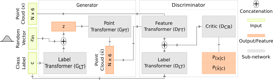
Figure 2: Given a random vector $z_{in}$ and class label $c$, the generator produces a colored point cloud $\hat{x}$. The real point cloud $x$, class label $c$, and the generated point cloud $\hat{x}$ are given to the discriminator which then tries to predict the probability of the data being real or synthetic. Best viewed in color.

5.1 Generator

The generator $G$ takes as input a random vector, $z_{in}\in\mathcal{N}(0,1)$, along with a class label $c\in C$ represented as one hot vector. The class label controls the generation of colored point clouds of a desired class. The generator is comprised of two sub-networks: a label transformer $G_{LT}$ and a point transformer $G_{PT}$.

The class label goes through $G_{LT}$, a shallow two-layer perceptron, and a class vector $g_{c}\in\mathbb{R}^{64}$ is constructed. The input vector $z_{in}$ is then concatenated with $g_{c}$ to produce a point vector $z$ which is given to $G_{PT}$ as input, i.e.,

$$z=(z_{in},g_{c}).$$

Following [40], the point transformer incorporates tree structured graph convolutions (TreeGCN). As the name suggests, information in TreeGCN is passed from the root node to a leaf node instead of all neighbors, i.e., the $i$-th node at layer $l$ is generated by aggregating information from its ancestors $A=\{a_{i}^{l-1},a_{i}^{l-2},\ldots,a_{i}^{1},a_{i}^{0}\}$. However, we have empirically found that the information from up to three immediate ancestors $A=\{a_{i}^{l-1},a_{i}^{l-2},a_{i}^{l-3}\}$ is sufficient for realistic point cloud generation. This observation improves the overall computational cost of our network as $G_{PT}$ is not bounded by the entire depth of the tree as in [40] (additional details and an analysis are included in Section 6). Therefore, the output of $(l+1)$-layer of $G_{PT}$ is a first order approximation of the Chebyshev expansion

$$p_{i}^{l+1}=\sigma\Bigg{(}\textbf{F}_{m}^{l}(p_{i}^{l})+\sum_{q_{j}\in A(p_{i}^{l})}W_{j}^{l}q_{j}^{l}+b^{l}\Bigg{)},$$

where

$$\textbf{F}_{m}^{l}(p_{i}^{l})=\sum_{j=1}^{m}S_{j}p_{i}^{l}+r_{j},$$

$\sigma(\cdot)$ is an activation function, $p_{i}^{l}$ is the $i$-th node of the graph at the $l$-layer, and $q_{j}^{l}$ is the $j$-th ancestor of $p_{i}^{l}$ from the set of three immediate ancestors of $p_{i}^{l}$. $W,b,S,r$ are learnable parameters and $\textbf{F}_{m}$ is a sub-network with $m$ support.

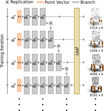
Figure 3: The progressive growing of the point transformer $G_{PT}$. The network starts with a leaf output layer and branches $(B_{1}\ldots,B_{T})$, each incorporating a tree graph, and converts a point vector $z$ into a low-resolution point cloud. After a predefined number of iterations, the number of branches is increased through the replication $R$ of the last branch $B_{T}$. In this figure, $T$ was kept small for visualization purposes. The process is continued until the generation of a point cloud at the desired resolution is achieved. Best viewed in color.

Figure 3 presents an overview of the progressive growing of PCGAN. We have sub-divided the point transformer $G_{PT}$ into two parts, a branch $B$ and a leaf $L$, where a leaf acts as the output layer of $G_{PT}$ for increasing replications $R$. Each branch incorporates a tree graph of expanding depth, $H=(h_{1},\ldots,h_{T})$, where $T$ is the total number of branches. The leaf also incorporates a tree graph of depth $h_{L}$. First, we optimize the generator to produce a point cloud $\hat{x}$ at a predefined base resolution $(N_{R_{1}}\times 6)$ where $R_{1}=h_{L}\Pi_{i=1}^{T}h_{i}$. After a fixed number of iterations, we introduce a new branch $B_{T+1}$ through the replication of the branch $B_{T}$ and we increase the depth $H=(h_{1},\ldots,h_{T+1})$ of the incorporated tree graph. The replication of an already optimized branch facilitates the generation of higher resolution point clouds without starting the learning process from scratch. We continue this procedure until the desired resolution of the point cloud is realized, i.e., $R_{d}=h_{L}\Pi_{i=1}^{T+d}h_{i}$.

5.2 Discriminator

Given a point cloud $x$, the discriminator $D$ tries to predict the probability of $x$ being real or synthesized. The discriminator is comprised of the following three sub-networks: a feature transformer $D_{FT}$, a label transformer $D_{LT}$, and a critic $D_{CR}$. The feature transformer network was inspired by [45] to collect local and global features through a dynamic graph construction. Nonetheless, we expand the feature size in every layer to account for the color of the point clouds.

Given an input point vector, each layer of the point transformer network constructs a dynamic $k$-NN graph, $\mathcal{G}^{l}=(\mathcal{V}^{l},\mathcal{E}^{l})$, with self loops. Each point of the point cloud represents a vertex in the graph and the vertex of each subsequent layer depends on the output of the preceding layers. For a graph $\mathcal{G}^{l}$ at layer $l$, the edges $e_{i}^{l}$ between a vertex $v_{i}^{l}$ and its $k$ nearest neighbors are defined as a nonlinear function $\Theta=[\theta_{1},\ldots,\theta_{m}]$ with learnable parameter $\theta$,

$$e_{i,(1,\ldots,k)}^{l}=\Theta_{j\in(1,\ldots,k)}(v_{i}^{l},v_{j}^{l}).$$

Although there are three choices available for $\Theta$, we use the function defined in [45] to capture both local and global features. Concretely, for two vertices $v_{i}$ and $v_{j}$ we have

$$\Theta(v_{i},v_{j})=\theta(v_{i},v_{i}-v_{j}).$$

Lastly, the output of the feature transform network is a feature vector $f_{c}$ collected from the channel-wise maximum operation on the edge features from all the edges of each vertex,

$$f_{c}=\max_{(i,j)\in\mathcal{E}}\Theta(v_{i},v_{j}).$$

The label transformer of the discriminator functions in an analogous way to the label transformer of the generator and it provides a label vector $d_{c}$. Note that even though $D_{LT}$ and $G_{LT}$ are similar in architecture, their objectives are distinct. Hence, we use two different networks for this reason. The feature vector $f_{c}$ together with the label vector $d_{c}$ are fed to the critic, a fully-connected three layer sub-network that aspires to predict the probability of its input vector being real or synthetic given that it was collected from object class $c$, i.e.,

$$D_{CR}(f_{c},d_{c})=[P(\text{real}\,|\,c),P(\text{generated}\,|\,c)].$$

6 Experiments

In this section, we describe our experimental setup and provide an analysis of the results.

Dataset. We used the synthetic dataset ShapeNetCore [10] to conduct our experiments. ShapeNetCore is a collection of CAD models of various object classes among which we chose Chair, Table, Sofa, Airplane, and Motorcycle for our experiments. We have selected these classes for the diversity of their shapes and we keep the number of classes to five to reduce the training time. In addition, we have eliminated any CAD model that does not have material/color information. The training data was prepared by collecting point clouds of desired resolution from the surface of the CAD models. We normalized each point cloud such that the object is centralized in a unit cube and the RGB colors are in the range $[-0.5,+0.5]$. Table 1 shows the number of sample objects in each class.

Class Label	Number of Samples
Airplane	4029
Chair	4064
Table	8474
Sofa	3149
Motorcycle	333

Table 1: The class labels and the number of samples in the training data.

Implementation Details. The generator of PCGAN learns to produce colored point clouds from low to high resolutions. We start the generation process with $N_{R_{1}}=1024$ points and double the number of points progressively. To save memory and reduce computation time, we fix $N_{R_{d}}=8192$ points as the highest resolution for the point clouds. The input to the generator is a vector, $z_{in}\in\mathbb{R}^{64}$, sampled from a normal distribution $z_{in}\in\mathcal{N}(0,1)$, and the labels of the chosen classes $c\in C$.

For the point transformer, the number of branches was set to $T=5$ with depth increments $H=[1,2,2,2,2]$. The leaf increments were set to $h_{L}=64$. The depth increment hyperparameter for the branches and the leaves is similar to the branching of [40]. The feature dimension for the layers of $G_{PT}$ was set to $[128,128,256,256,128,128,6]$. We used the Xavier initialization [14] for $G_{PT}$ and the support $q$ for each branch was set to $10$ as in [40].

The feature dimension for the layers of the feature transform sub-network were set to $[6,64,128,256,512,1024]$. To comply with the constraints of WGAN-GP, we did not use any batch normalization or dropout in $D_{FT}$. For $D_{FT}$, $k=20$ was used to construct the $k$-NN graph and $k$ was increased by $10$ with each increment in resolution.

For both the generator and the discriminator, LeakyReLU nonlinearity with a negative slope of 0.2 was employed. The learning rate $\alpha$ was set to $10^{-4}$ and the Adam optimizer [24] with coefficients $\beta_{1}=0.0$ and $\beta_{2}=0.95$ were used. The gradient penalty coefficient $\lambda$ for WGAN-GP was set to 10.

Metrics. To quantitatively evaluate generated samples in 2D, the Frèchet inception distance [18] is the most commonly used metric. We propose a similar metric called the Frèchet dynamic distance (FDD) to evaluate the generated point clouds where DGCNN [45] is used as a feature extractor. Although similar metrics exist [40, 41] where PointNet is used to extract features, the color of the point clouds is not considered and they suffer from the limitations of PointNet.

We use DGCNN because it collects both local and global information over the feature space and it also performs better than PointNet in point cloud classification [45]. To implement FDD, we trained DGCNN until a 98% test accuracy per class was achieved on the task of classification. Then, we extracted a $512$-dimensional feature vector from the average pooling layer of DGCNN to calculate the mean vector and covariance matrix. For real point clouds $x$ and synthetic point clouds $\hat{x}$, the FDD calculates the 2-Wasserstein distance,

$$\text{FDD}(x,\hat{x})=\|\mu_{x}-\mu_{\hat{x}}\|+\operatorname{tr}(\Sigma_{x}+\Sigma_{\hat{x}}-2(\Sigma_{x}\Sigma_{\hat{x}})^{1/2}),$$

where $\mu$ and $\Sigma$ represent the mean vector and the covariance matrix, respectively. The matrix trace is denoted by $\operatorname{tr}()$. Additionally, we have used the matrices from Achlioptas et al. [1] for point cloud evaluation and we have compared the results with [1, 40, 43].

Class	Model	JSD $\downarrow$	MMD-CD $\downarrow$	MMD-EMD $\downarrow$	COV-CD $\uparrow$	COV-EMD $\uparrow$
	r-GAN (dense)	0.182	0.0009	0.094	31	9
	r-GAN (conv)	0.350	0.0008	0.101	26	7
Airplane	Valsesia et al. (no up.)	0.164	0.0010	0.102	24	13
	Valsesia et al. (up.)	0.083	0.0008	0.071	31	14
	tree-GAN	0.097	0.0004	0.068	61	20
	PCGAN (ours)	0.085	0.0010	0.070	37	29
	r-GAN (dense)	0.238	0.0029	0.136	33	13
	r-GAN (conv)	0.517	0.0030	0.223	23	4
Chair	Valsesia et al. (no up.)	0.119	0.0033	0.104	26	20
	Valsesia et al. (up.)	0.100	0.0029	0.097	30	26
	tree-GAN	0.119	0.0016	0.101	58	30
	PCGAN (ours)	0.089	0.0027	0.093	30	33
	r-GAN (dense)	0.221	0.0020	0.146	32	12
	r-GAN(conv)	0.293	0.0025	0.110	21	12
Sofa	Valsesia et al. (no up.)	0.095	0.0024	0.094	25	19
	Valsesia et al. (up.)	0.063	0.0020	0.083	39	24
	PCGAN (ours)	0.16	0.0027	0.093	24	27
Motorcycle	PCGAN (ours)	0.25	0.0016	0.097	10	9
Table	PCGAN (ours)	0.093	0.0035	0.089	45	43

Table 2: A qualitative evaluation of the Jensen-Shannon divergence (JSD), the minimum matching distance (MMD), coverage (COV) with the Earth mover’s distance (EMD), and the pseudo-chamfer distance (CD). Please refer to [1] for details regarding the metrics. The results of previous studies are from [40, 43]. The magenta and cyan values denote the best and the second best results, respectively. The resolution of the evaluated point clouds was $2048\times 3$.

Class	Real Data	Generated Samples
Airplane	$1.12\times 10^{-5}$	4.58
Chair	$2.07\times 10^{-9}$	3.07
Motorcycle	$1.04\times 10^{-4}$	13.25
Sofa	$5.88\times 10^{-6}$	3.14
Table	$4.37\times 10^{-7}$	2.02

Table 3: The FDD score for point cloud samples generated by PCGAN. Notice that the scores for real point clouds are almost zero. The point clouds were evaluated at a resolution of $8192\times 6$.

6.1 Results

A set of synthesized objects along with their real counterparts is shown in Figure 4. As is evident from the samples, our model first learns the basic structure of an object in low resolutions and gradually builds up to higher resolutions. PCGAN also learns the relationship between object parts and color. For example, the legs of the chair have equal colors while the seat/arms are a different color, the legs of the table have matching colors while the top is a contrasting color, and the airplane wings/engine have the same color while the body/tail has a dissimilar color.

Quantitative Analysis. We generated $5000$ random samples for each class and performed an evaluation using the matrices from [1]. Table 2 presents our findings along with comparisons to previous studies [1, 40, 43]. Note that although our model is capable of generating higher resolutions and colors, we only used point clouds with $N=2048$ points in order to be comparable with other methods. Also, separate models were trained in [1, 40, 43] to generate point clouds of different classes while we have used the same model to generate point clouds for all five classes. Even though we have achieved comparable results in Table 2, the main focus of our work is dense colored point cloud generation and point clouds with a resolution of $N=2048$ is an intermediate result of our network. We have also evaluated colored dense point clouds ($N=8192$) using the proposed FDD metric with the results presented in Table 3.

Computational Complexity. Tree structured graph convolutions are used in each layer of the point transformer sub-network. Since every subsequent node in the tree is originally dependent upon all of its ancestors, the time complexity of the graph convolutions is $\sum_{l=1}^{L}B\times n_{i}^{l}\times A^{l}_{i}\times V^{l}_{i}$, where $B$ is the batch size of the training data, $L$ is the total number of layers, $n_{i}^{l}$ is the height of the tree graph at the $i$-th node, $A_{i}$ is the induced number of ancestors preceding $i$-th node, and $V_{i}^{l}$ is the induced vertex number of the $i$-th node [40]. However, we restrict $G_{PT}$ to aggregate information from at most three levels of ancestors in each layer. Thus, $n_{i}^{l}\leq 3$ and the effective time complexity is $\sum_{l=1}^{L}B\times 3\times A^{l}_{i}\times V^{l}_{i}$.

Progressive Experiments. We have experimented with different strategies of progressive growing such as branching $H=[2,4,4,4],[1,2,4,8],[1,2,4,2]$ and leaf $h_{L}=[4,16,64]$ increments. Although branching and leaf combinations may generate more discernible point cloud geometries and colors for individual classes, we have found that $H=[1,2,2,2]$ and $h_{L}=64$ work best in our experiments. Additionally, instead of creating new branches we have experimented with introducing new leaves for progressive growing. However, this seems to destabilize the network and results in the generation of inferior samples.

Limitations and Future Work. The main drawback of our model is the computational complexity. With $\approx 20000$ point clouds from five classes, our model takes roughly $15$ minutes per iteration (MPI) on four Nvidia GTX 1080 GPUs to generate point clouds $\hat{x}\in\mathbb{R}^{1024\times 6}$. The MPI rises with every increase in resolution. For future work, we will attempt to reduce the computational complexity of our network. Our model also struggles with generating objects that have fewer examples in the training data. The generated point clouds of the Motorcycle class in Figure 4 is an example of this (ShapeNetCore has only $333$ CAD models of the Motorcycle). In the future, we will try to improve the generalization ability of our model and we will work on the addition of surface normal estimates.

7 Conclusion

This paper introduces PCGAN, the first conditional generative adversarial network to generate dense colored point clouds in an unsupervised mode. To reduce the complexity of the generation process, we train our network in a coarse to fine way with progressive growing and we condition our network on class labels for multiclass point cloud creation. We evaluate both point cloud geometry and color using our new FDD metric. In addition, we provide comparisons on point cloud geometry with recent generation techniques using available metrics. The evaluation results show that our model is capable of synthesizing high-quality point clouds for a disparate array of object classes.

Figure 4: The results of generated samples produced by PCGAN. Our model first learns the basic structure of an object at low resolutions and gradually builds up towards high-level details. The relationship between the object parts and their colors (e.g., the legs of the chair/table are the same color while seat/top are contrasting) is also learned by the network. Mitsuba 2 [37] was used to render the point clouds. Best viewed in color.

References

- [1] P. Achlioptas, O. Diamanti, I. Mitliagkas, and L. Guibas. Learning representations and generative models for 3d point clouds. In International Conference on Machine Learning, pages 40–49, 2018.
- [2] E. Ahmed, A. Saint, A. E. R. Shabayek, K. Cherenkova, R. Das, G. Gusev, D. Aouada, and B. Ottersten. A survey on deep learning advances on different 3d data representations. arXiv preprint arXiv:1808.01462, 2018.
- [3] M. Arjovsky, S. Chintala, and L. Bottou. Wasserstein gan. arXiv preprint arXiv:1701.07875, 2017.
- [4] M. Atzmon, H. Maron, and Y. Lipman. Point convolutional neural networks by extension operators. arXiv preprint arXiv:1803.10091, 2018.
- [5] J. Biswas and M. Veloso. Depth camera based indoor mobile robot localization and navigation. In IEEE International Conference on Robotics and Automation, pages 1697–1702, 2012.
- [6] R. Bostelman, P. Russo, J. Albus, T. Hong, and R. Madhavan. Applications of a 3d range camera towards healthcare mobility aids. In IEEE International Conference on Networking, Sensing and Control, pages 416–421, 2006.
- [7] X. Cao and K. Nagao. Point cloud colorization based on densely annotated 3d shape dataset. In International Conference on Multimedia Modeling, pages 436–446. Springer, 2019.
- [8] X. Cao, W. Wang, K. Nagao, and R. Nakamura. Psnet: A style transfer network for point cloud stylization on geometry and color. In IEEE Winter Conference on Applications of Computer Vision, pages 3337–3345, 2020.
- [9] Z. Cao, Q. Huang, and R. Karthik. 3d object classification via spherical projections. In International Conference on 3D Vision (3DV), pages 566–574. IEEE, 2017.
- [10] A. X. Chang, T. Funkhouser, L. Guibas, P. Hanrahan, Q. Huang, Z. Li, S. Savarese, M. Savva, S. Song, H. Su, et al. Shapenet: An information-rich 3d model repository. arXiv preprint arXiv:1512.03012, 2015.
- [11] S. Chaudhuri, D. Ritchie, K. Xu, and H. Zhang. Learning generative models of 3d structures. Eurographics Tutorial, 2019.
- [12] B. Eckart, K. Kim, A. Troccoli, A. Kelly, and J. Kautz. Accelerated generative models for 3d point cloud data. In Proceedings of the IEEE Conference on Computer Vision and Pattern Recognition, pages 5497–5505, 2016.
- [13] M. Gadelha, R. Wang, and S. Maji. Multiresolution tree networks for 3d point cloud processing. In Proceedings of the European Conference on Computer Vision (ECCV), pages 103–118, 2018.
- [14] X. Glorot and Y. Bengio. Understanding the difficulty of training deep feedforward neural networks. In Proceedings of the Thirteenth International Conference on Artificial Intelligence and Statistics, pages 249–256, 2010.
- [15] I. Goodfellow, J. Pouget-Abadie, M. Mirza, B. Xu, D. Warde-Farley, S. Ozair, A. Courville, and Y. Bengio. Generative adversarial nets. In Advances in Neural Information Processing Systems, pages 2672–2680, 2014.
- [16] I. Gulrajani, F. Ahmed, M. Arjovsky, V. Dumoulin, and A. C. Courville. Improved training of wasserstein gans. In Advances in Neural Information Processing Systems, pages 5767–5777, 2017.
- [17] A. Hertz, R. Hanocka, R. Giryes, and D. Cohen-Or. Pointgmm: a neural gmm network for point clouds. In Proceedings of the IEEE/CVF Conference on Computer Vision and Pattern Recognition, pages 12054–12063, 2020.
- [18] M. Heusel, H. Ramsauer, T. Unterthiner, B. Nessler, and S. Hochreiter. Gans trained by a two time-scale update rule converge to a local nash equilibrium. In Advances in Neural Information Processing Systems, pages 6626–6637, 2017.
- [19] J. Hou, A. Dai, and M. Nießner. 3d-sis: 3d semantic instance segmentation of rgb-d scans. In Proceedings of the IEEE Conference on Computer Vision and Pattern Recognition, pages 4421–4430, 2019.
- [20] A. Ioannidou, E. Chatzilari, S. Nikolopoulos, and I. Kompatsiaris. Deep learning advances in computer vision with 3d data: A survey. ACM Computing Surveys (CSUR), 50(2):1–38, 2017.
- [21] T. Karras, T. Aila, S. Laine, and J. Lehtinen. Progressive growing of gans for improved quality, stability, and variation. arXiv preprint arXiv:1710.10196, 2017.
- [22] T. Karras, S. Laine, and T. Aila. A style-based generator architecture for generative adversarial networks. In Proceedings of the IEEE Conference on Computer Vision and Pattern Recognition, pages 4401–4410, 2019.
- [23] T. Karras, S. Laine, M. Aittala, J. Hellsten, J. Lehtinen, and T. Aila. Analyzing and improving the image quality of stylegan. In Proceedings of the IEEE/CVF Conference on Computer Vision and Pattern Recognition, pages 8110–8119, 2020.
- [24] D. P. Kingma and J. Ba. Adam: A method for stochastic optimization. arXiv preprint arXiv:1412.6980, 2014.
- [25] C.-L. Li, M. Zaheer, Y. Zhang, B. Poczos, and R. Salakhutdinov. Point cloud gan. arXiv preprint arXiv:1810.05795, 2018.
- [26] J. Li, B. M. Chen, and G. Hee Lee. So-net: Self-organizing network for point cloud analysis. In Proceedings of the IEEE Conference on Computer Vision and Pattern Recognition, pages 9397–9406, 2018.
- [27] B. Liu, M. Guo, E. Chou, R. Mehra, S. Yeung, N. L. Downing, F. Salipur, J. Jopling, B. Campbell, K. Deru, et al. 3d point cloud-based visual prediction of icu mobility care activities. In Machine Learning for Healthcare Conference, pages 17–29, 2018.
- [28] R. C. Luo, V. W. Ee, and C.-K. Hsieh. 3d point cloud based indoor mobile robot in 6-dof pose localization using fast scene recognition and alignment approach. In International Conference on Multisensor Fusion and Integration for Intelligent Systems (MFI), pages 470–475. IEEE, 2016.
- [29] D. Maturana and S. Scherer. Voxnet: A 3d convolutional neural network for real-time object recognition. In IEEE/RSJ International Conference on Intelligent Robots and Systems (IROS), pages 922–928, 2015.
- [30] K. Mo, P. Guerrero, L. Yi, H. Su, P. Wonka, N. Mitra, and L. J. Guibas. Structurenet: Hierarchical graph networks for 3d shape generation. arXiv preprint arXiv:1908.00575, 2019.
- [31] https://github.com/robotic-vision-lab/Progressive-Conditional-Generative-Adversarial-Network.
- [32] A. Pfrunder, P. V. Borges, A. R. Romero, G. Catt, and A. Elfes. Real-time autonomous ground vehicle navigation in heterogeneous environments using a 3d lidar. In IEEE/RSJ International Conference on Intelligent Robots and Systems (IROS), pages 2601–2608, 2017.
- [33] S. T. Pöhlmann, E. F. Harkness, C. J. Taylor, and S. M. Astley. Evaluation of kinect 3d sensor for healthcare imaging. Journal of Medical and Biological Engineering, 36(6):857–870, 2016.
- [34] C. R. Qi, H. Su, K. Mo, and L. J. Guibas. Pointnet: Deep learning on point sets for 3d classification and segmentation. In Proceedings of the IEEE Conference on Computer Vision and Pattern Recognition, pages 652–660, 2017.
- [35] C. R. Qi, L. Yi, H. Su, and L. J. Guibas. Pointnet++: Deep hierarchical feature learning on point sets in a metric space. In Advances in Neural Information Processing Systems, pages 5099–5108, 2017.
- [36] S. Ramasinghe, S. Khan, N. Barnes, and S. Gould. Spectral-gans for high-resolution 3d point-cloud generation. arXiv preprint arXiv:1912.01800, 2019.
- [37] Realistic Graphics Lab, EPFL. Mitsuba 2 renderer, 2020. http://www.mitsuba-renderer.org.
- [38] M. Sarmad, H. J. Lee, and Y. M. Kim. Rl-gan-net: A reinforcement learning agent controlled gan network for real-time point cloud shape completion. In Proceedings of the IEEE Conference on Computer Vision and Pattern Recognition, pages 5898–5907, 2019.
- [39] G. Sharma, E. Kalogerakis, and S. Maji. Learning point embeddings from shape repositories for few-shot segmentation. In International Conference on 3D Vision (3DV), pages 67–75. IEEE, 2019.
- [40] D. W. Shu, S. W. Park, and J. Kwon. 3d point cloud generative adversarial network based on tree structured graph convolutions. In Proceedings of the IEEE International Conference on Computer Vision, pages 3859–3868, 2019.
- [41] Y. Sun, Y. Wang, Z. Liu, J. Siegel, and S. Sarma. Pointgrow: Autoregressively learned point cloud generation with self-attention. In IEEE Winter Conference on Applications of Computer Vision, pages 61–70, 2020.
- [42] L. P. Tchapmi, V. Kosaraju, H. Rezatofighi, I. Reid, and S. Savarese. Topnet: Structural point cloud decoder. In Proceedings of the IEEE Conference on Computer Vision and Pattern Recognition, pages 383–392, 2019.
- [43] D. Valsesia, G. Fracastoro, and E. Magli. Learning localized generative models for 3d point clouds via graph convolution. In International Conference on Learning Representations, 2018.
- [44] C. Villani. Optimal transport: old and new, volume 338. Springer Science & Business Media, 2008.
- [45] Y. Wang, Y. Sun, Z. Liu, S. E. Sarma, M. M. Bronstein, and J. M. Solomon. Dynamic graph cnn for learning on point clouds. ACM Transactions On Graphics (TOG), 38(5):1–12, 2019.
- [46] Y. Wang, D. J. Tan, N. Navab, and F. Tombari. Forknet: Multi-branch volumetric semantic completion from a single depth image. In Proceedings of the IEEE International Conference on Computer Vision, pages 8608–8617, 2019.
- [47] Y. Wang, S. Zhang, B. Wan, W. He, and X. Bai. Point cloud and visual feature-based tracking method for an augmented reality-aided mechanical assembly system. The International Journal of Advanced Manufacturing Technology, 99(9-12):2341–2352, 2018.
- [48] X. Wen, T. Li, Z. Han, and Y.-S. Liu. Point cloud completion by skip-attention network with hierarchical folding. In Proceedings of the IEEE/CVF Conference on Computer Vision and Pattern Recognition, pages 1939–1948, 2020.
- [49] M. Whitty, S. Cossell, K. S. Dang, J. Guivant, and J. Katupitiya. Autonomous navigation using a real-time 3d point cloud. In Australasian Conference on Robotics and Automation, pages 1–3, 2010.
- [50] J. Wu, C. Zhang, X. Zhang, Z. Zhang, W. T. Freeman, and J. B. Tenenbaum. Learning shape priors for single-view 3d completion and reconstruction. In Proceedings of the European Conference on Computer Vision (ECCV), pages 646–662, 2018.
- [51] W. Wu, Z. Qi, and L. Fuxin. Pointconv: Deep convolutional networks on 3d point clouds. In Proceedings of the IEEE Conference on Computer Vision and Pattern Recognition, pages 9621–9630, 2019.
- [52] J. Xie, Y. Xu, Z. Zheng, S.-C. Zhu, and Y. Nian Wu. Generative pointnet: Energy-based learning on unordered point sets for 3d generation, reconstruction and classification. arXiv, pages arXiv–2004, 2020.
- [53] G. Yang, X. Huang, Z. Hao, M.-Y. Liu, S. Belongie, and B. Hariharan. Pointflow: 3d point cloud generation with continuous normalizing flows. In Proceedings of the IEEE International Conference on Computer Vision, pages 4541–4550, 2019.
- [54] Y. Yang, C. Feng, Y. Shen, and D. Tian. Foldingnet: Point cloud auto-encoder via deep grid deformation. In Proceedings of the IEEE Conference on Computer Vision and Pattern Recognition, pages 206–215, 2018.
- [55] L. Yi, H. Su, X. Guo, and L. J. Guibas. Syncspeccnn: Synchronized spectral cnn for 3d shape segmentation. In Proceedings of the IEEE Conference on Computer Vision and Pattern Recognition, pages 2282–2290, 2017.
- [56] L. Yi, W. Zhao, H. Wang, M. Sung, and L. J. Guibas. Gspn: Generative shape proposal network for 3d instance segmentation in point cloud. In Proceedings of the IEEE conference on computer vision and pattern recognition, pages 3947–3956, 2019.
- [57] W. Yuan, T. Khot, D. Held, C. Mertz, and M. Hebert. Pcn: Point completion network. In International Conference on 3D Vision (3DV), pages 728–737. IEEE, 2018.
- [58] M. Zaheer, S. Kottur, S. Ravanbakhsh, B. Poczos, R. R. Salakhutdinov, and A. J. Smola. Deep sets. In Advances in Neural Information Processing Systems, pages 3391–3401, 2017.
- [59] Y. Zhou and O. Tuzel. Voxelnet: End-to-end learning for point cloud based 3d object detection. In Proceedings of the IEEE Conference on Computer Vision and Pattern Recognition, pages 4490–4499, 2018.
- [60] Q. Zhu, L. Chen, Q. Li, M. Li, A. Nüchter, and J. Wang. 3d lidar point cloud based intersection recognition for autonomous driving. In IEEE Intelligent Vehicles Symposium, pages 456–461, 2012.