Meta-Active Learning for Node Response Prediction in Graphs

Abstract

Meta-learning is an important approach to improve machine learning performance with a limited number of observations for target tasks. However, when observations are unbalancedly obtained, it is difficult to improve the performance even with meta-learning methods. In this paper, we propose an active learning method for meta-learning on node response prediction tasks in attributed graphs, where nodes to observe are selected to improve performance with as few observed nodes as possible. With the proposed method, we use models based on graph convolutional neural networks for both predicting node responses and selecting nodes, by which we can predict responses and select nodes even for graphs with unseen response variables. The response prediction model is trained by minimizing the expected test error. The node selection model is trained by maximizing the expected error reduction with reinforcement learning. We demonstrate the effectiveness of the proposed method with 11 types of road congestion prediction tasks.

1 Introduction

A wide variety of data are represented as graphs, such as road networks [43, 23], citation graphs [11], metabolic pathways [35], ecosystem [54], and social networks [68]. In this paper, we consider node response prediction tasks, where a response value for each node is predicted given an attributed graph. Node response prediction is an important task, which includes congestion prediction with a road network [45, 9], scientific paper classification with a citation graph [72], and user preference prediction with a social network [32, 67].

As the number of nodes with observed responses increases, the performance of node response prediction is improved in general. However, a sufficient number of observed responses are often unavailable since obtaining responses requires high cost, e.g., placing sensors at many roads, and manually labeling by experts with domain knowledge. For improving performance with a small number of observations, many meta-learning methods have been proposed [59, 4, 51, 1, 66, 62, 3, 16, 46, 38, 17, 56, 73, 14, 22, 37, 27, 5, 52, 53, 64, 49, 71, 42]. Meta-learning is to learn a model that can predict unseen response variables with only a few observed nodes. However, when observed nodes are unbalancedly placed in a graph, e.g., observations are obtained with nodes that are directly connected to each other and no observations are given with other distant nodes, it is difficult to improve the prediction performance even with meta-learning methods.

In this paper, we propose an active learning method to select nodes to observe in an attributed graph so that the prediction performance is improved with as few observed nodes as possible. We assume that many attributed graphs with observed responses are given as a training dataset. Our task is to improve the node response prediction performance with fewer observations in an unseen attributed graph with an unseen response variable. The proposed method contains two models: a response prediction model, and node selection model. The response prediction model predicts node responses given an attributed graph, and the node selection model outputs scores for selecting a node to observe given an attributed graph. Figure 1 illustrates the response prediction and node selection models. We use graph convolutional neural networks (GCNs) [40] for both of the models. By taking attributes, observed responses, and masks that indicating observed nodes as input, the GCNs can output predictions or scores for unseen graphs depending on the observed responses by aggregating information of all nodes considering the graph structure.

The response prediction model is trained by minimizing the expected test prediction error using an episodic training framework [51, 57, 62, 16, 46]. The episodic training framework, which is often used for meta-learning, simulates a test phase by randomly selecting observed and unobserved nodes using training attributed graphs. The node selection model is trained by maximizing the expected test error reduction by reinforcement learning. Although many existing active learning methods use heuristics, such as uncertainty [44, 28, 74, 33, 20], for selecting node policies, our meta-learning framework directly optimizes an active learning policy that maximizes the expected test error reduction, where the policy is applicable to unseen graphs with unseen response variables. Figure 1 illustrates our training framework.

Our main contributions are as follows:

• We propose a meta-active learning method for node response prediction in graphs, where our models can be used for unseen graphs with unseen response variables.

• The proposed method directly maximizes the expected test error reduction for node response prediction tasks.

• We demonstrate the effectiveness of the proposed method using 11 types of road congestion prediction tasks.

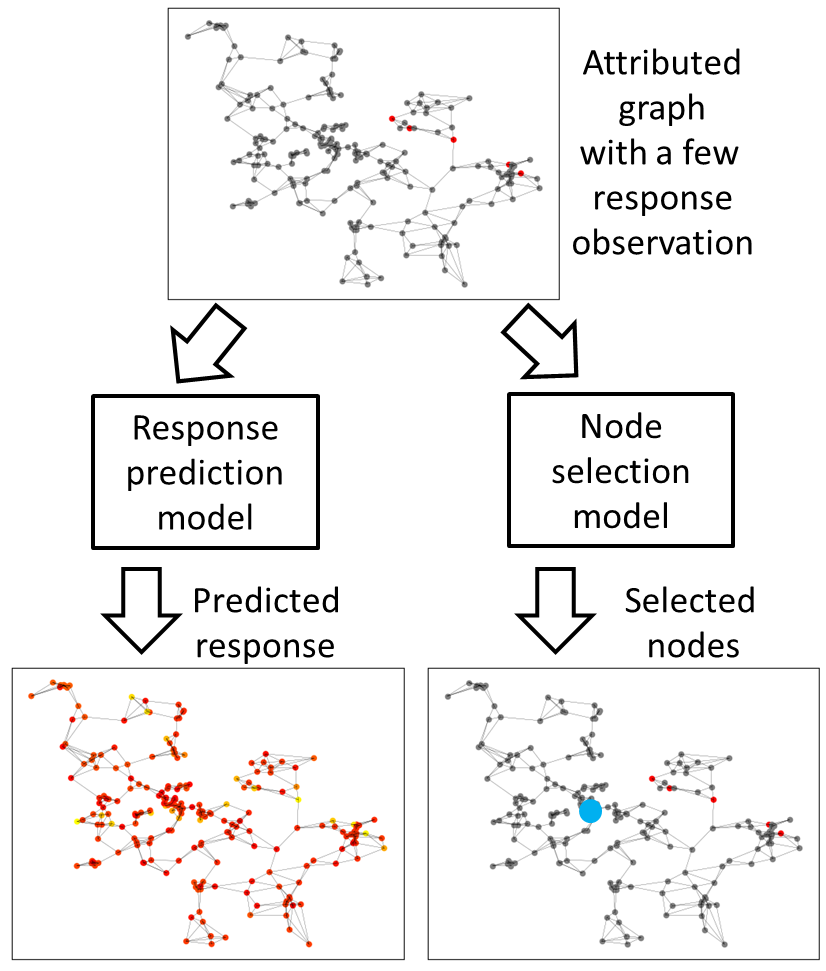
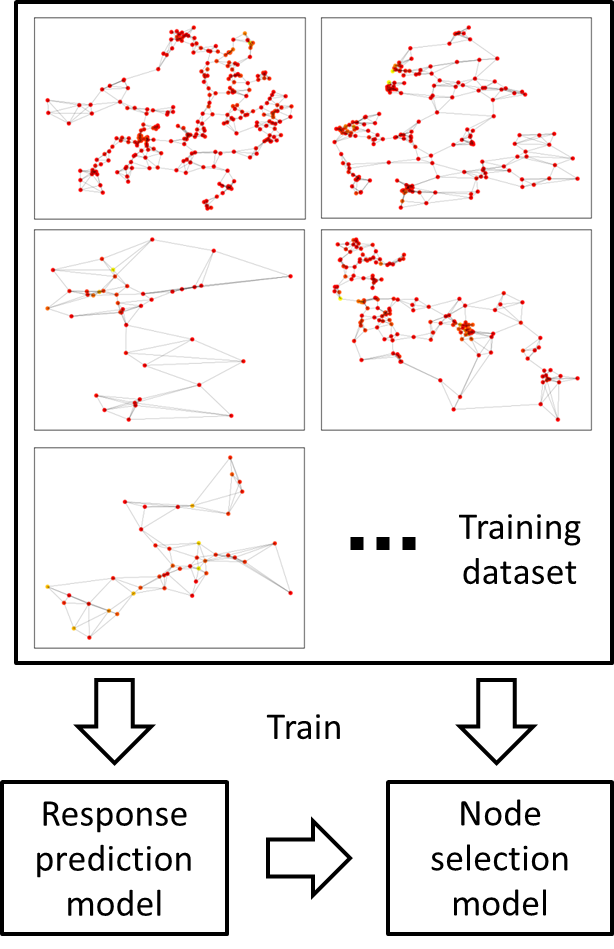
(a) Models	(b) Training

Figure 1: (a) Our response prediction and node selection models. These models take attributed graphs with a few response observations as input, where observed and unobserved nodes are represented by red and gray circles. The response prediction model outputs predicted responses for each node, where red (yellow) indicates high (low) predicted values. The node selection model outputs scores for each node that are used for selecting nodes to observe in active learning, where a selected node is represented by the big blue circle. (b) Our training framework. First, the response prediction model is trained using a training dataset, which contains various graphs with various response types. Second, the node selection model is trained using the training dataset and trained response prediction model.

The remainder of this paper is organized as follows. Section 2 briefly reviews related work. Section 3 defines our problem, proposes our response prediction and node selection models, and presents their training procedures. In Section 4, we demonstrate the effectiveness of the proposed method with congestion prediction tasks using road graphs in the UK. Finally, we give a concluding remark and future work in Section 5.

2 Related work

Active learning selects examples to be labeled for improving the performance while reducing costly labeling effort. Many active learning methods have been proposed [19], such uncertainty sampling [44, 28, 74, 33, 20], query-by-committee [61, 18], mutual information [24, 29, 31], core-set [60], and mean standard deviation [36, 34]. Although the metrics used in these methods are computed efficiently, they are different from the expected test error that we want to minimize. Active learning methods that directly reduce the test error have been proposed [8, 55]. These methods use simple models that can calculate the test error in closed form [8], or use sampling to estimate the test error [55]. On the other hand, the proposed method directly optimizes a policy that maximizes the test error reduction, by which we do not need to calculate the test error in a test phase. Although a number of active learning methods using reinforcement learning have been proposed [15, 47, 48, 26, 41, 50, 13, 30, 2, 70], but they are not for graphs. Active learning for graph embedding has been proposed [7] but it is not for node response prediction tasks. GCNs have been in a wide variety of applications [58, 40, 10, 12, 25], including meta-learning [6, 21]. However, they are not used for active learning.

3 Proposed method

3.1 Problem definition

In a training phase, we are given a set of $D$ graphs with attributes and responses, $\mathcal{G}=\{\mathbf{G}_{d}\}_{d=1}^{D}$, where $\mathbf{G}_{d}=(\mathbf{A}_{d},\mathbf{X}_{d},\mathbf{y}_{d})$ is the $d$th graph, $\mathbf{A}_{d}\in\{0,1\}^{N_{d}\times N_{d}}$ is the adjacency matrix, $N_{d}$ is the number of nodes, $\mathbf{X}_{d}=(\mathbf{x}_{dn})_{n=1}^{N_{d}}\in\mathbb{R}^{N_{d}\times J_{d}}$, $\mathbf{y}_{d}=(y_{dn})_{n=1}^{N_{d}}\in\mathbb{R}^{N_{d}}$, $\mathbf{x}_{dn}\in\mathbb{R}^{J_{d}}$ is the attributes of the $n$th node, and $y_{dn}\in\mathbb{R}$ is its response. Although we assume undirected and unweighted graphs for simplicity, we can straightforwardly extend the proposed method for directed and/or weighted graphs. In a test phase, we are given target graph $\mathbf{G}_{*}=(\mathbf{A}_{*},\mathbf{X}_{*})$ without responses. The response type of the target graph is different from that of the training graphs, e.g., the target response variable is bicycle traffic, and the training response variables are car, taxis and bus traffic. Our task is to improve the response prediction performance of all nodes in the target graph by selecting nodes to observe, where a smaller number of observed nodes is preferred.

3.2 Model

Graph convolutional neural networks (GCNs) are used for modeling both predicting responses and selecting nodes to observe. Let $\mathbf{m}_{d}\in\{0,1\}^{N_{d}}$ be the binary mask vector for indicating observed nodes, where $m_{dn}=1$ if the response of the $n$th node is observed, and $m_{dn}=0$ otherwise. Let $\bar{\mathbf{y}}_{d}$ be the observed response vector, where $\bar{y}_{dn}=y_{dn}$ if $m_{dn}=1$, $\bar{y}_{dn}=0$ otherwise. For the input of a GCN, we use the following concatenated vector of the attributes, observed responses, and masks,

$$\mathbf{z}_{dn}^{(0)}=[\mathbf{x}_{dn},\bar{y}_{dn},m_{dn}],$$ (1)

where $\mathbf{z}_{dn}^{(0)}$ is the input vector of the $n$th node, and $[\cdot,\cdot]$ represents a concatenation. With the above input, we can output predictions and scores without retraining even when responses of nodes are additionally observed by changing the input such that $\bar{y}_{dn}=y_{dn}$ and $m_{dn}=1$ for additionally observed node $n$.

With GCNs, the hidden state at the next layer is calculated by

$$\mathbf{z}_{dn}^{(k+1)}=\sigma\left(\mathbf{W}^{(k)}\mathbf{z}_{dn}^{(k)}+\frac{1}{N_{dn}}\sum_{m=1}^{N_{d}}a_{dnm}\mathbf{U}^{(k)}\mathbf{z}_{dm}^{(k)}\right),$$ (2)

where $\mathbf{z}_{dn}^{(k)}$ is the hidden state of the $n$th node at the $k$th layer, $\sigma$ is the activation function, $a_{dnm}$ is the $(n,m)$th element of adjacency matrix $\mathbf{A}_{d}$, $N_{dn}=\sum_{m}a_{dnm}$ is the number of neighbors of the $n$th node, $\mathbf{W}^{(k)}\in\mathbb{R}^{H_{k+1}\times H_{k}}$ and $\mathbf{U}^{(k)}\in\mathbb{R}^{H_{k+1}\times H_{k}}$ are the linear projection matrices of the $k$th layer, and $H_{k}$ is the hidden state size of the $k$th layer. Eq. (2) aggregates the information of the own node (the first term) and its neighbor nodes (the second term) with transformation. The hidden state at the last $K$th layer is the output of the GCN.

We use a GCN for response prediction model $f$ with parameters $\bm{\Phi}=\{\mathbf{W}_{\mathrm{f}}^{(k)},\mathbf{U}_{\mathrm{f}}^{(k)}\}_{k=1}^{K_{\mathrm{f}}}$ as follows,

$$\hat{\mathbf{y}}_{d}=f(\mathbf{G}_{d},\mathbf{m}_{d};\bm{\Phi}),$$ (3)

where $\hat{\mathbf{y}}_{d}\in\mathbb{R}^{N_{d}}$ is the predicted responses, and the $K_{\mathrm{f}}$ is the number of layers. The input of the GCN in Eq. (1) is calculated using $\mathbf{G}_{d}$ and $\mathbf{m}_{d}$. Also, we use another GCN for node selection model $g$ with parameters $\bm{\Theta}=\{\mathbf{W}_{\mathrm{g}}^{(k)},\mathbf{U}_{\mathrm{g}}^{(k)}\}_{k=1}^{K_{\mathrm{g}}}$ as follows,

$$\mathbf{s}_{d}=g(\mathbf{G}_{d},\mathbf{m}_{d};\bm{\Theta}),$$ (4)

where $\mathbf{s}_{d}=(s_{dn})_{n=1}^{N_{d}}\in\mathbb{R}^{N_{d}}$, and $s_{dn}$ is the score that the $n$th node is selected to observe the response.

Our model can be used for meta-learning, where values of unseen response variables are predicted, since it has similar operations to existing meta-learning methods, such as conditional neural processes [22]. Conditional neural processes consist of an encoder, an aggregator, and a decoder. The encoder takes observed attributes and responses as input, and outputs a representation for each observed node. The aggregator summarizes the set of representations for the observed nodes into a single representation. The decoder takes the aggregated representation and attributes without responses as input, and predicts responses. Since our model takes the attributes, observed responses, and masks as input, the GCN simultaneously works as an encoder, aggregator, and decoder. In particular, the first term in Eq. (2) works as an encoder for nodes with observed responses, and as a decoder for nodes without observed responses. The second term in Eq. (2) works as an aggregator by summarizing representations of the neighbor nodes.

3.3 Training

First, we train parameters $\bm{\Phi}$ of response prediction model $f$, and then train parameters $\bm{\Theta}$ of node selection model $g$ while fixing $f$.

3.3.1 Response prediction model

We estimate parameters $\bm{\Phi}$ of response prediction model $f$ in Eq. (3) by minimizing the expected test prediction error,

$$\hat{\bm{\Phi}}=\arg\min_{\bm{\Phi}}\mathbb{E}_{\mathbf{G}_{d}}[\mathbb{E}_{\mathbf{m}_{d}}[L(\mathbf{G}_{d},\mathbf{m}_{d};\bm{\Phi})]],$$ (5)

using training graph set $\mathcal{G}$ with an episodic training framework. Here, $\mathbb{E}$ represents an expectation, and the expectation are taken over various graphs $\mathbf{G}_{d}$ in training graph set $\mathcal{G}$, and over various observation patterns $\mathbf{m}_{d}$ in each graph, where we randomly generate target graphs for simulating a test phase. The test prediction error for a target graph is calculated by

$$L(\mathbf{G}_{d},\mathbf{m}_{d};\bm{\Phi})=\frac{1}{\sum_{n=1}^{N_{d}}(1-m_{dn})}\sum_{n=1}^{N_{d}}(1-m_{dn})\parallel y_{dn}-f_{n}(\mathbf{G}_{d},\mathbf{m}_{d};\bm{\Phi})\parallel^{2},$$ (6)

where $f_{n}(\mathbf{G}_{d},\mathbf{m}_{d};\bm{\Phi})$ is the $n$th element of the output of the response prediction model, the responses are predicted using the observed nodes, $m_{dn}=1$, and the test prediction error is calculated for the unobserved nodes, $m_{dn}=0$. When response variables are categorical, the cross-entropy loss with the softmax function can be used instead of the squared error loss.

Algorithm 1 shows the training procedures of the response prediction model. For each epoch, we simulate a test phase by uniform randomly sampling a graph from the training dataset (Line 3) and uniform randomly selecting observed nodes in the graph (Line 4).

Algorithm 1 Training procedure of response prediction model $f$.

0:  Set of training graphs $\mathcal{G}$, support set size $N_{\mathrm{S}}$

0:  Trained model parameters $\bm{\Phi}$

1:  Initialize parameters $\bm{\Phi}$ randomly

2:  while not done do

3:     Sample graph $\mathbf{G}_{d}$ from $\mathcal{G}$

4:     Sample $N_{\mathrm{S}}$ observed nodes $\mathcal{S}$ from $\{1,\cdots,N_{d}\}$

5:     Set mask vector $\mathbf{m}_{d}$ using the sampled observed nodes, such that $m_{dn}=1$ if $n\in\mathcal{S}$, and $m_{dn}=0$ otherwise

6:     Calculate loss $L(\mathbf{G}_{d},\mathbf{m}_{d};\bm{\Phi})$ by Eq. (6) and its gradients

7:     Update parameters $\bm{\Phi}$ using the gradients

8:  end while

3.3.2 Node selection model

We estimate parameters $\bm{\Theta}$ of node selection model $g$ in Eq. (4) by maximizing the expected test error reduction using training graph set $\mathcal{G}$ based on reinforcement learning with an episodic training framework. For rewards, we use the test error reduction when node $n$ is selected to observe with graph $\mathbf{G}_{d}$ and mask $\mathbf{m}_{d}$ as follows,

$$R(\mathbf{G}_{d},\mathbf{m}_{d},n)=\frac{L(\mathbf{G}_{d},\mathbf{m}_{d};\hat{\bm{\Phi}})-L(\mathbf{G}_{d},\mathbf{m}_{d}^{(+n)};\hat{\bm{\Phi}})}{L(\mathbf{G}_{d},\mathbf{m}_{d};\hat{\bm{\Phi}})},$$ (7)

where $\mathbf{m}_{d}^{(+n)}$ is the updated mask vector of $\mathbf{m}_{d}$ when node $n$ is additionally observed, $m_{dn^{\prime}}^{(+n)}=1$ if $n^{\prime}=n$, and $m_{dn^{\prime}}^{(+n)}=m_{dn^{\prime}}$ otherwise. Here, parameters of trained response prediction models $\hat{\bm{\Phi}}$ is used. We can calculate the error $L(\mathbf{G}_{d},\mathbf{m}_{d}^{(+n)};\hat{\bm{\Phi}})$ when node $n$ is additionally observed by feeding the updated mask vector and graph into our response prediction model based on GCNs without retraining. In terms of reinforcement learning, a pair of graph $\mathbf{G}_{d}$ and mask $\mathbf{m}_{d}$ is a state, node to observe $n$ is an action, and node selection model $g(\mathbf{G}_{d},\mathbf{m}_{d};\bm{\Theta})$ that outputs scores of actions given a state is a policy. The expected test error reduction is calculated by

$$\hat{\bm{\Theta}}=\arg\max_{\bm{\Theta}}\mathbb{E}_{\mathbf{G}_{d}}[\mathbb{E}_{(\mathbf{m},n)\sim\bm{\pi}(\bm{\Theta})}[R(\mathbf{G}_{d},\mathbf{m},n)]],$$ (8)

where $\bm{\pi}(\bm{\Theta})$ is the probability distribution of the policy for selecting nodes, which is defined by node selection model $g$ with parameter $\bm{\Theta}$.

Algorithm 2 shows the training procedures of the node selection model with policy gradients, where active learning is simulated using randomly selected graphs (Line 3). Each active learning task starts with a graph without observed responses (Line 4), and we iterate until $N_{\mathrm{A}}$ nodes are observed (Line 5). A node is selected according to the following policy that is calculated from scores $\mathbf{s}_{d}$ (Lines 6–7),

$$\pi_{dn}=\frac{\exp(s^{\prime}_{dn})}{\sum_{m=1}^{N_{d}}\exp(s^{\prime}_{dm})},$$ (9)

where $s^{\prime}_{dn}=s_{dn}$ if $m_{dn}=0$, and $s^{\prime}_{dn}=-\infty$ otherwise, by which already observed nodes are excluded from selection. A node is sampled according to the categorical distribution with parameters $\bm{\pi}_{d}$ (Line 8). The test error reduction, or reward, is calculated at Line 9. At Line 10, parameters $\bm{\Phi}$ are updated by using the log-derivative trick, or Reinforce [69], where the average total reward was used for the baseline [75]. Although we use the myopic rewards in the algorithm, we can also use non-myopic rewards.

Algorithm 2 Training procedure of node selection model $g$.

0:  Set of training graphs $\mathcal{G}$, maximum support set size $N_{\mathrm{A}}$

0:  Trained model parameters $\bm{\Theta}$

1:  Initialize parameters $\bm{\Theta}$ randomly

2:  while not done do

3:     Sample graph $\mathbf{G}_{d}$ from $\mathcal{G}$

4:     Initialize mask vector $\mathbf{m}_{d}=\bm{0}$

5:     for $t=1,\cdots,N_{\mathrm{A}}$ do

6:        Calculate score $\mathbf{s}_{d}=g(\mathbf{G}_{d},\mathbf{m}_{d};\bm{\Theta})$

7:        Set policy $\bm{\pi}_{d}$ by Eq. (9)

8:        Sample an observed node according to the policy $n\sim\mathrm{Categorical}(\bm{\pi}_{d})$

9:        Calculate test error reduction $R(\mathbf{G}_{d},\mathbf{m}_{d},n)$ by Eq. (7)

10:        Update parameters $\bm{\Theta}\leftarrow\bm{\Theta}+\alpha R(\mathbf{G}_{d},\mathbf{m}_{d},n)\nabla_{\bm{\Theta}}\log\pi_{dn}$

11:        Update mask to include selected node $n$ in observed nodes $m_{dn}=1$

12:     end for

13:  end while

3.4 Test

In a test phase, given target $\mathbf{G}_{*}$ without responses, we first initialize mask vector $\mathbf{m}_{*}=\bm{0}$. Second, we select a node with the maximum score

$$\hat{n}=\arg\max_{n:m_{*n}=0}s_{*n},$$ (10)

among unobserved nodes using the trained node selection model. Third, we update the mask vector with the selected node by $m_{*\hat{n}}=1$. We iterate the second and third steps until an end condition is satisfied.

4 Experiments

4.1 Data

We evaluated the proposed method with 11 types of congestion prediction tasks using road graphs in the UK. The original data were obtained from UK Department for Transport . The data contained road level Annual Average Daily Flow (AADF) at major and minor roads in the UK for the following 11 types: pedal cycles, two-wheeled motor vehicles, car and taxis, buses and coaches, light goods vehicles (LGVs), two-rigid axle heavy good vehicle (HGVs), three-rigid axle HGVs, four or more rigid axle HGVs, three or four-articulated axle HGVs, five-articulated axle HGVs, and six-articulated axle HGVs. We used the 11 AADFs for response variables, and used road categories, road types, longitude and latitude for attributes. There were six road categories, and two road types (major and minor). These categorical attributes were transformed to one-hot vectors. The real-valued attributes and responses were normalized in the range of zero to one. We generated an undirected road graph for each local authority, where a node was a road, and nodes with four nearest neighbors based on their latitude and longitude were connected with edges. Examples of the generated road graphs are shown in Figure 1. There were 206 graphs in total for each response variable and for each year, where the average, minimum and maximum number of nodes for each graph was 103, 5 and 562. For each experiment, we used an AADF in a region for target data, and used the other AADFs in the other regions for training and validation data; i.e., the AADF or region in target data are not contained in training and validation data. There were 11 regions, such as East-Midlands, London, Scotland and Wales. A region was used for validation, and the remaining nine regions were used for training.

4.2 Comparing methods

We compared the proposed active learning method with the following methods for selecting nodes to observe: Random, Variance, Entropy, MI (mutual information), and FF (feed-forward neural network). All the methods used the same response prediction model in Eq. (3) to evaluate the active learning performance. The Random method randomly selects a node to observe.

The Entropy method selects a node that maximizes the entropy, or uncertainty [44, 28, 74, 33, 20]. With the entropy method, first, we trained a GCN that outputs mean and standard deviation of responses,

$$\hat{\mathbf{y}}_{d},\hat{\bm{\sigma}}_{d}=f_{\mathrm{entropy}}(\mathbf{G}_{d},\mathbf{m}_{d};\bm{\Phi}),$$ (11)

by minimizing the negative Gaussian likelihood loss instead of the test prediction error in Eq. (6),

$$L_{\mathrm{entropy}}(\mathbf{G}_{d},\mathbf{m}_{d};\bm{\Phi})=\frac{1}{\sum_{n=1}^{N_{d}}(1-m_{dn})}\sum_{n=1}^{N_{d}}(1-m_{dn})\log\mathcal{N}(y_{dn};\hat{y}_{dn},\hat{\sigma}_{dn}^{2}),$$ (12)

where $\mathcal{N}(x;\mu,\sigma^{2})$ is the probability density function at $x$ of the Gaussian distribution with mean $\mu$ and standard deviation $\sigma$, and $\hat{y}_{dn}$ and $\hat{\sigma}_{dn}$ are the estimated mean and standard deviation for the $n$th node by Eq. (11). The GCN in Eq. (11) is the same with Eq. (3) except that its final layer additionally outputs standard deviation. Using the trained GCN in Eq. (11), we select a node that maximizes the entropy, $\hat{n}=\arg\max_{n:m_{*n}}\mathbb{H}[y_{dn}|\mathbf{G}_{d},\mathbf{m}_{d}]$, where the entropy is calculated by

$$\mathbb{H}[y_{dn}|\mathbf{G}_{d},\mathbf{m}_{d}]=\log\hat{\sigma}_{dn}+\frac{1}{2}(\log(2\pi)+1).$$ (13)

The Variance method selects a node that maximizes the variance estimated using dropout [65]. Dropout randomly sets hidden unit activities to zero [63]. Let $\hat{y}_{dn}^{(\ell)}\in\mathbb{R}^{N_{d}}$ be the $\ell$th output of the GCN in Eq. (3) in stochastic runs with dropout. The variance of prediction $\hat{y}_{dn}$ was calculated by

$$\mathrm{Var}[\hat{y}_{dn}]=\frac{1}{L}\sum_{\ell=1}^{L}(\hat{y}_{dn}^{(\ell)}-\bar{\hat{y}}_{dn})^{2},$$ (14)

where $L$ is the number of stochastic runs, $\bar{\hat{y}}_{dn}=\frac{1}{L}\sum_{\ell=1}^{L}\hat{y}_{dn}^{(\ell)}$ is the average over the stochastic runs. We used $L=10$.

The MI method selects a node that maximizes the mutual infromation [20] between responses and model parameters,

$$\mathbb{I}[y_{dn},\bm{\Phi}|\mathbf{G}_{d},\mathbf{m}_{d}]=\mathbb{H}[y_{dn}|\mathbf{G}_{d},\mathbf{m}_{d}]-\mathbb{E}_{p(\bm{\Phi}|\mathbf{G}_{d},\mathbf{m}_{d})}[\mathbb{H}[y_{dn}|\mathbf{G}_{d},\mathbf{m}_{d},\bm{\Phi}]].$$ (15)

The first term was calculated with Eq. (13). The second term was calculated using dropout as follows,

$$\mathbb{E}_{p(\bm{\Phi}|\mathbf{G}_{d},\mathbf{m}_{d})}[\mathbb{H}[y_{dn}|\mathbf{G}_{d},\mathbf{m}_{d},\bm{\Phi}]]=\frac{1}{L}\sum_{\ell=1}^{L}(\log\hat{\sigma}_{dn}^{(\ell)}+\frac{1}{2}(\log(2\pi)+1))),$$ (16)

where $\hat{\sigma}_{dn}^{(\ell)}$ is the $\ell$th estimate of the standard deviation by Eq. (11) in stochastic runs with dropout.

The FF method used feed-forward neural networks for the node selection model instead of Eq. (4) based on GCNs. The FF method takes attributes $\mathbf{x}_{dn}$, and outputs score $s_{dn}$ for each node. The neural networks were trained in the same way with the proposed method. Since the FF method outputs the score for each node individually, it does not meta-learn, but learns the relationship between the attributes and scores.

4.3 Proposed method setting

With GCNs for response prediction and node selection models, the number of hidden units was 32, the number of layers was three with residual connections. The models were trained by Adam [39] with learning rate $10^{-3}$ and dropout rate $0.1$. The maximum number of epochs was 1,000, and the validation data were used for early stopping. The support set size was $N_{\mathrm{S}}=5$ for training response prediction models, and the maximum support set size was $N_{\mathrm{A}}=10$ for training node selection models.

4.4 Results

Figure 2 shows the mean squared error and its standard error with different numbers of observations for each AADF prediction task. All the methods decreased the error as the number of observed nodes increased, which implied that the response prediction model improved the performance by observing node responses. The proposed method achieved the lowest mean squared error in most cases. This result indicates that training node selection models by directly maximizing test reduction errors using reinforcement learning is effective. The Entropy method achieved the second lowest error. Even if we observed a node has high entropy, the test errors for other nodes might not decrease when the observed node has little relationships with other nodes. On the other hand, the proposed method selects nodes so as to maximize the test error reduction by considering the information of all nodes by GCNs. The MI and Variance methods did not perform well. This result implies that the estimation of variance and entropy based on dropout is difficult in this task. Since the FF method cannot use the information of other nodes, it performed badly. The computational time for training node selection and response prediction models with the proposed method was 3.7 and 44.5 hours, respectively, by computers with 2.10-GHz Xeon Gold 6130 CPU.

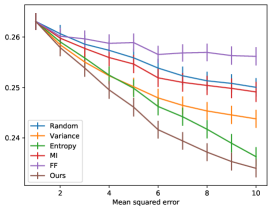
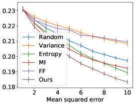
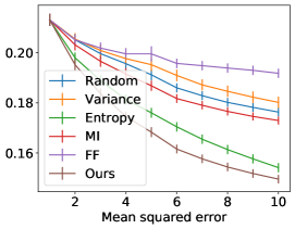
(a) pedal cycles	(b) two-wheeled	(c) car
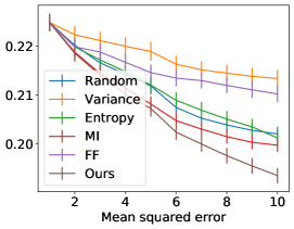
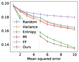
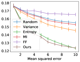
(d) buses and coaches	(e) LGVs	(f) 2-rigid
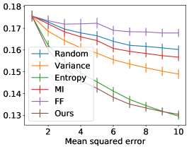
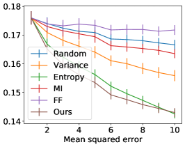
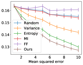
(g) 3-rigid	(h) 4-rigid	(i) 3-articulated
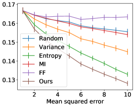
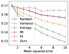
(j) 5-articulated	(k) 6-articulated

Figure 2: Test mean squared error (vertical axis) with different numbers of observations (horizontal axis) for each AADF task. The bar shows the standard error.

5 Conclusion

We proposed an active learning method for meta-learning on node response prediction tasks in graph data. With the proposed method, graph convolutional neural networks are used for calculating scores to select nodes to observe, where attributes, observed responses, and masks indicating observed nodes are taken as input. By using the graph convolutional neural networks, we can select nodes for unseen graphs with unseen response variables depending on a few observed responses and the graph structure. We demonstrated that the proposed method achieved higher performance for road congestion prediction tasks with fewer observed nodes compared with existing active learning methods. For future work, we want to apply the proposed method to tasks other than node response prediction, such as link prediction and graph generation. Although we used graph convolutional neural networks, we plan to use other meta-learning models for meta-active learning.

References

- [1] M. Andrychowicz, M. Denil, S. Gomez, M. W. Hoffman, D. Pfau, T. Schaul, B. Shillingford, and N. De Freitas. Learning to learn by gradient descent by gradient descent. In Advances in Neural Information Processing Systems, pages 3981–3989, 2016.
- [2] P. Bachman, A. Sordoni, and A. Trischler. Learning algorithms for active learning. In Proceedings of the 34th International Conference on Machine Learning-Volume 70, pages 301–310, 2017.
- [3] S. Bartunov and D. Vetrov. Few-shot generative modelling with generative matching networks. In International Conference on Artificial Intelligence and Statistics, pages 670–678, 2018.
- [4] Y. Bengio, S. Bengio, and J. Cloutier. Learning a synaptic learning rule. In International Joint Conference on Neural Networks, 1991.
- [5] J. Bornschein, A. Mnih, D. Zoran, and D. J. Rezende. Variational memory addressing in generative models. In Advances in Neural Information Processing Systems, pages 3920–3929, 2017.
- [6] A. J. Bose, A. Jain, P. Molino, and W. L. Hamilton. Meta-graph: Few shot link prediction via meta learning. arXiv preprint arXiv:1912.09867, 2019.
- [7] H. Cai, V. W. Zheng, and K. C.-C. Chang. Active learning for graph embedding. arXiv preprint arXiv:1705.05085, 2017.
- [8] D. A. Cohn, Z. Ghahramani, and M. I. Jordan. Active learning with statistical models. Journal of Artificial Intelligence Research, 4:129–145, 1996.
- [9] Z. Cui, K. Henrickson, R. Ke, and Y. Wang. Traffic graph convolutional recurrent neural network: A deep learning framework for network-scale traffic learning and forecasting. IEEE Transactions on Intelligent Transportation Systems, 2019.
- [10] M. Defferrard, X. Bresson, and P. Vandergheynst. Convolutional neural networks on graphs with fast localized spectral filtering. In Advances in Neural Information Processing Systems, pages 3844–3852, 2016.
- [11] Y. Ding. Scientific collaboration and endorsement: Network analysis of coauthorship and citation networks. Journal of Informetrics, 5(1):187–203, 2011.
- [12] D. K. Duvenaud, D. Maclaurin, J. Iparraguirre, R. Bombarell, T. Hirzel, A. Aspuru-Guzik, and R. P. Adams. Convolutional networks on graphs for learning molecular fingerprints. In Advances in Neural Information Processing Systems, pages 2224–2232, 2015.
- [13] S. Ebert, M. Fritz, and B. Schiele. Ralf: A reinforced active learning formulation for object class recognition. In 2012 IEEE Conference on Computer Vision and Pattern Recognition, pages 3626–3633. IEEE, 2012.
- [14] H. Edwards and A. Storkey. Towards a neural statistician. arXiv preprint arXiv:1606.02185, 2016.
- [15] M. Fang, Y. Li, and T. Cohn. Learning how to active learn: A deep reinforcement learning approach. arXiv preprint arXiv:1708.02383, 2017.
- [16] C. Finn, P. Abbeel, and S. Levine. Model-agnostic meta-learning for fast adaptation of deep networks. In Proceedings of the 34th International Conference on Machine Learning, pages 1126–1135, 2017.
- [17] C. Finn, K. Xu, and S. Levine. Probabilistic model-agnostic meta-learning. In Advances in Neural Information Processing Systems, pages 9516–9527, 2018.
- [18] Y. Freund, H. S. Seung, E. Shamir, and N. Tishby. Selective sampling using the query by committee algorithm. Machine learning, 28(2-3):133–168, 1997.
- [19] Y. Fu, X. Zhu, and B. Li. A survey on instance selection for active learning. Knowledge and Information Systems, 35(2):249–283, 2013.
- [20] Y. Gal, R. Islam, and Z. Ghahramani. Deep bayesian active learning with image data. In Proceedings of the 34th International Conference on Machine Learning, pages 1183–1192, 2017.
- [21] V. Garcia and J. Bruna. Few-shot learning with graph neural networks. arXiv preprint arXiv:1711.04043, 2017.
- [22] M. Garnelo, D. Rosenbaum, C. Maddison, T. Ramalho, D. Saxton, M. Shanahan, Y. W. Teh, D. Rezende, and S. A. Eslami. Conditional neural processes. In International Conference on Machine Learning, pages 1690–1699, 2018.
- [23] X. Geng, Y. Li, L. Wang, L. Zhang, Q. Yang, J. Ye, and Y. Liu. Spatiotemporal multi-graph convolution network for ride-hailing demand forecasting. In Proceedings of the AAAI Conference on Artificial Intelligence, volume 33, pages 3656–3663, 2019.
- [24] C. Guestrin, A. Krause, and A. P. Singh. Near-optimal sensor placements in Gaussian processes. In Proceedings of the 22nd International Conference on Machine Learning, pages 265–272, 2005.
- [25] W. Hamilton, Z. Ying, and J. Leskovec. Inductive representation learning on large graphs. In Advances in Neural Information Processing Systems, pages 1024–1034, 2017.
- [26] M. Haussmann, F. A. Hamprecht, and M. Kandemir. Deep active learning with adaptive acquisition. arXiv preprint arXiv:1906.11471, 2019.
- [27] L. B. Hewitt, M. I. Nye, A. Gane, T. Jaakkola, and J. B. Tenenbaum. The variational homoencoder: Learning to learn high capacity generative models from few examples. arXiv preprint arXiv:1807.08919, 2018.
- [28] A. Holub, P. Perona, and M. C. Burl. Entropy-based active learning for object recognition. In 2008 IEEE Computer Society Conference on Computer Vision and Pattern Recognition Workshops, pages 1–8. IEEE, 2008.
- [29] N. Houlsby, F. Huszár, Z. Ghahramani, and M. Lengyel. Bayesian active learning for classification and preference learning. arXiv preprint arXiv:1112.5745, 2011.
- [30] W.-N. Hsu and H.-T. Lin. Active learning by learning. In AAAI Conference on Artificial Intelligence, 2015.
- [31] T. Iwata, N. Houlsby, and Z. Ghahramani. Active learning for interactive visualization. In Artificial Intelligence and Statistics, pages 342–350, 2013.
- [32] M. Jamali and M. Ester. A matrix factorization technique with trust propagation for recommendation in social networks. In Proceedings of the fourth ACM Conference on Recommender Systems, pages 135–142, 2010.
- [33] F. Jing, M. Li, H.-J. Zhang, and B. Zhang. Entropy-based active learning with support vector machines for content-based image retrieval. In 2004 IEEE International Conference on Multimedia and Expo (ICME)(IEEE Cat. No. 04TH8763), volume 1, pages 85–88. IEEE, 2004.
- [34] M. Kampffmeyer, A.-B. Salberg, and R. Jenssen. Semantic segmentation of small objects and modeling of uncertainty in urban remote sensing images using deep convolutional neural networks. In Proceedings of the IEEE Conference on Computer Vision and Pattern Recognition Workshops, pages 1–9, 2016.
- [35] M. Kanehisa and S. Goto. KEGG: Kyoto encyclopedia of genes and genomes. Nucleic Acids Research, 28(1):27–30, 2000.
- [36] A. Kendall, V. Badrinarayanan, and R. Cipolla. Bayesian segnet: Model uncertainty in deep convolutional encoder-decoder architectures for scene understanding. arXiv preprint arXiv:1511.02680, 2015.
- [37] H. Kim, A. Mnih, J. Schwarz, M. Garnelo, A. Eslami, D. Rosenbaum, O. Vinyals, and Y. W. Teh. Attentive neural processes. arXiv preprint arXiv:1901.05761, 2019.
- [38] T. Kim, J. Yoon, O. Dia, S. Kim, Y. Bengio, and S. Ahn. Bayesian model-agnostic meta-learning. In Advances in Neural Information Processing Systems, 2018.
- [39] D. P. Kingma and J. Ba. ADAM: A method for stochastic optimization. In International Conference on Learning Representations, 2015.
- [40] T. N. Kipf and M. Welling. Semi-supervised classification with graph convolutional networks. arXiv preprint arXiv:1609.02907, 2016.
- [41] K. Konyushkova, R. Sznitman, and P. Fua. Learning active learning from data. In Advances in Neural Information Processing Systems, pages 4225–4235, 2017.
- [42] B. M. Lake. Compositional generalization through meta sequence-to-sequence learning. In Advances in Neural Information Processing Systems, pages 9788–9798, 2019.
- [43] S. Lämmer, B. Gehlsen, and D. Helbing. Scaling laws in the spatial structure of urban road networks. Physica A: Statistical Mechanics and its Applications, 363(1):89–95, 2006.
- [44] D. D. Lewis and W. A. Gale. A sequential algorithm for training text classifiers. In Proceedings of the 17th Annual International ACM SIGIR Conference on Research and Development in Information Retrieval, pages 3–12, 1994.
- [45] Y. Li, R. Yu, C. Shahabi, and Y. Liu. Diffusion convolutional recurrent neural network: Data-driven traffic forecasting. arXiv preprint arXiv:1707.01926, 2017.
- [46] Z. Li, F. Zhou, F. Chen, and H. Li. Meta-SGD: Learning to learn quickly for few-shot learning. arXiv preprint arXiv:1707.09835, 2017.
- [47] M. Liu, W. Buntine, and G. Haffari. Learning how to actively learn: A deep imitation learning approach. In Proceedings of the 56th Annual Meeting of the Association for Computational Linguistics (Volume 1: Long Papers), pages 1874–1883, 2018.
- [48] M. Liu, W. Buntine, and G. Haffari. Learning to actively learn neural machine translation. In Proceedings of the 22nd Conference on Computational Natural Language Learning, pages 334–344, 2018.
- [49] J. Narwariya, P. Malhotra, L. Vig, G. Shroff, and T. Vishnu. Meta-learning for few-shot time series classification. In Proceedings of the 7th ACM IKDD CoDS and 25th COMAD, pages 28–36. 2020.
- [50] K. Pang, M. Dong, Y. Wu, and T. Hospedales. Meta-learning transferable active learning policies by deep reinforcement learning. arXiv preprint arXiv:1806.04798, 2018.
- [51] S. Ravi and H. Larochelle. Optimization as a model for few-shot learning. In International Conference on Learning Representations, 2017.
- [52] S. Reed, Y. Chen, T. Paine, A. v. d. Oord, S. Eslami, D. Rezende, O. Vinyals, and N. de Freitas. Few-shot autoregressive density estimation: Towards learning to learn distributions. arXiv preprint arXiv:1710.10304, 2017.
- [53] D. J. Rezende, S. Mohamed, I. Danihelka, K. Gregor, and D. Wierstra. One-shot generalization in deep generative models. In Proceedings of the 33rd International Conference on International Conference on Machine Learning, pages 1521–1529, 2016.
- [54] F. S. Roberts. Food webs, competition graphs, and the boxicity of ecological phase space. In Theory and Applications of Graphs, pages 477–490. Springer, 1978.
- [55] N. Roy and A. McCallum. Toward optimal active learning through sampling estimation of error reduction. In Proceedings of the Eighteenth International Conference on Machine Learning, pages 441–448, 2001.
- [56] A. A. Rusu, D. Rao, J. Sygnowski, O. Vinyals, R. Pascanu, S. Osindero, and R. Hadsell. Meta-learning with latent embedding optimization. In International Conference on Learning Representations, 2019.
- [57] A. Santoro, S. Bartunov, M. Botvinick, D. Wierstra, and T. Lillicrap. Meta-learning with memory-augmented neural networks. In International Conference on Machine Learning, pages 1842–1850, 2016.
- [58] F. Scarselli, M. Gori, A. C. Tsoi, M. Hagenbuchner, and G. Monfardini. The graph neural network model. IEEE Transactions on Neural Networks, 20(1):61–80, 2008.
- [59] J. Schmidhuber. Evolutionary principles in self-referential learning. on learning now to learn: The meta-meta-meta…-hook. Master’s thesis, Technische Universitat Munchen, Germany, 1987.
- [60] O. Sener and S. Savarese. Active learning for convolutional neural networks: A core-set approach. arXiv preprint arXiv:1708.00489, 2017.
- [61] H. S. Seung, M. Opper, and H. Sompolinsky. Query by committee. In Proceedings of the fifth Annual Workshop on Computational Learning Theory, pages 287–294, 1992.
- [62] J. Snell, K. Swersky, and R. Zemel. Prototypical networks for few-shot learning. In Advances in Neural Information Processing Systems, pages 4077–4087, 2017.
- [63] N. Srivastava, G. Hinton, A. Krizhevsky, I. Sutskever, and R. Salakhutdinov. Dropout: a simple way to prevent neural networks from overfitting. Journal of Machine Learning Research, 15(1):1929–1958, 2014.
- [64] W. Tang, L. Liu, and G. Long. Few-shot time-series classification with dual interpretability. In ICML Time Series Workshop. 2019.
- [65] E. Tsymbalov, M. Panov, and A. Shapeev. Dropout-based active learning for regression. In Analysis of Images, Social Networks and Texts, pages 247–258, 2018.
- [66] O. Vinyals, C. Blundell, T. Lillicrap, D. Wierstra, et al. Matching networks for one shot learning. In Advances in Neural Information Processing Systems, pages 3630–3638, 2016.
- [67] F. E. Walter, S. Battiston, and F. Schweitzer. A model of a trust-based recommendation system on a social network. Autonomous Agents and Multi-Agent Systems, 16(1):57–74, 2008.
- [68] S. Wasserman and K. Faust. Social network analysis: Methods and applications, volume 8. Cambridge university press, 1994.
- [69] R. J. Williams. Simple statistical gradient-following algorithms for connectionist reinforcement learning. Machine learning, 8(3-4):229–256, 1992.
- [70] M. Woodward and C. Finn. Active one-shot learning. arXiv preprint arXiv:1702.06559, 2017.
- [71] Y. Xie, H. Jiang, F. Liu, T. Zhao, and H. Zha. Meta learning with relational information for short sequences. In Advances in Neural Information Processing Systems, pages 9901–9912, 2019.
- [72] Z. Yang, W. W. Cohen, and R. Salakhutdinov. Revisiting semi-supervised learning with graph embeddings. arXiv preprint arXiv:1603.08861, 2016.
- [73] H. Yao, Y. Wei, J. Huang, and Z. Li. Hierarchically structured meta-learning. In International Conference on Machine Learning, pages 7045–7054, 2019.
- [74] D. Yu, B. Varadarajan, L. Deng, and A. Acero. Active learning and semi-supervised learning for speech recognition: A unified framework using the global entropy reduction maximization criterion. Computer Speech & Language, 24(3):433–444, 2010.
- [75] T. Zhao, H. Hachiya, G. Niu, and M. Sugiyama. Analysis and improvement of policy gradient estimation. In Advances in Neural Information Processing Systems, pages 262–270, 2011.