Controlling Graph Dynamics with
Reinforcement Learning and Graph Neural Networks
Controlling Graph Dynamics with
Reinforcement Learning and Graph Neural Networks :
Supplementary Material
Abstract
We consider the problem of controlling a partially-observed dynamic process on a graph by a limited number of interventions. This problem naturally arises in contexts such as scheduling virus tests to curb an epidemic; targeted marketing in order to promote a product; and manually inspecting posts to detect fake news spreading on social networks.
We formulate this setup as a sequential decision problem over a temporal graph process. In face of an exponential state space, combinatorial action space and partial observability, we design a novel tractable scheme to control dynamical processes on temporal graphs. We successfully apply our approach to two popular problems that fall into our framework: prioritizing which nodes should be tested in order to curb the spread of an epidemic, and influence maximization on a graph.
1 Introduction
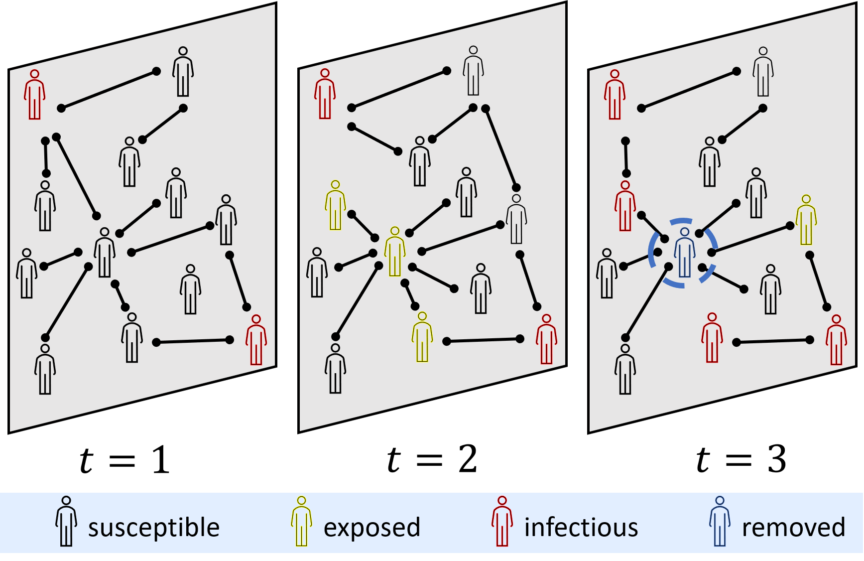
Consider an epidemic spreading in the population. To contain the disease and prevent it from spreading, it becomes critical to detect infected carriers and isolate them; see Fig. 1 for an illustration. As the epidemic spreads, the demand for tests outgrows their availability, and not all potential carriers can be tested. It becomes necessary to identify the most likely epidemic carriers using limited testing resources. How should we rank candidates and prioritize vaccines and tests to prevent the disease from spreading? As a second example, imagine a seemingly very different problem, where one would like to promote an opinion or support product adaption by advertisements or information sharing on a social graph. If an impactful node is convinced, it may influence other nodes towards the desired opinion, creating a cascade of information diffusion.
These two problems are important examples of a larger family of problems: controlling diffusive processes over networks through nodal interventions. Other examples include viruses inflicting computer networks or cascades of failures in power networks. In all these cases, an agent can steer the dynamics of the system using interventions that modify the states of a (relatively) small number of nodes. For instance, infected people can be asked to self-quarantine, preventing the spread of a disease, and key twitters may be targeted with coupons. However, a key difficulty is that the current state is often not fully observed, for example, we don’t know the ground truth infection status for every node in the graph.
More formally, we consider a graph whose structure changes in time. is the set of nodes and is the set of edges at step . The state of a node is a random variable that depends on the interactions between and its neighbors. At each turn, the agent may select a subset of nodes and attempt to change their state. The goal is to minimize an objective that depends on the number of nodes in each state. For example, consider a setup where the agent tries to promote its product or opinion. At each step, the agent may select a set of seed nodes and attempt to influence them by presenting relevant information or ads. If those nodes are convinced, they may spread the information through future contacts. The optimization goal, in this case, is to maximize the number of influenced nodes.
The problem of controlling the dynamics of a system using localized interventions is very hard, and for several reasons. First, it requires making decisions in a continuously changing environment with complex dependencies. Second, to solve the problem one must assess the potential downstream ripple effect for any specific node that becomes affected, and balance it with the probability that the node indeed becomes affected. Finally, models must handle noise and partial observability. In particular, it is well known that even the single-round, non-sequential, influence maximization problem is computationally hard (Kempe et al., 2003).
Current approaches for solving this problem can be divided into two main families: (1) Monte Carlo simulation that estimates the utility of each decision (see e.g. Goyal et al., 2011). These approaches can find good solutions for small to moderate-sized ( nodes) graphs, but do not scale to larger graphs. (2) Heuristics based on topological properties of the known graph. For example, act on nodes with a high degree (e.g. Liu et al., 2017). These approaches can be scaled to very large graphs, but are often sub-optimal. In addition to these two families, learning approaches have been used to mix different heuristics (Chung et al., 2019; Tian et al., 2020).
We pose the problem of controlling a diffusive process on a temporally evolving graph as a partially-observed Markov decision process (POMDP). We then formulate the problem of selecting a subset of nodes for dynamical intervention as a ranking problem, and design an actor-critic RL algorithm to solve it. We use the observed changes of nodes states and connections to construct a temporal multi-graph, which has time-stamped interactions over edges, and describe a deep architecture based on GNNs to process it.
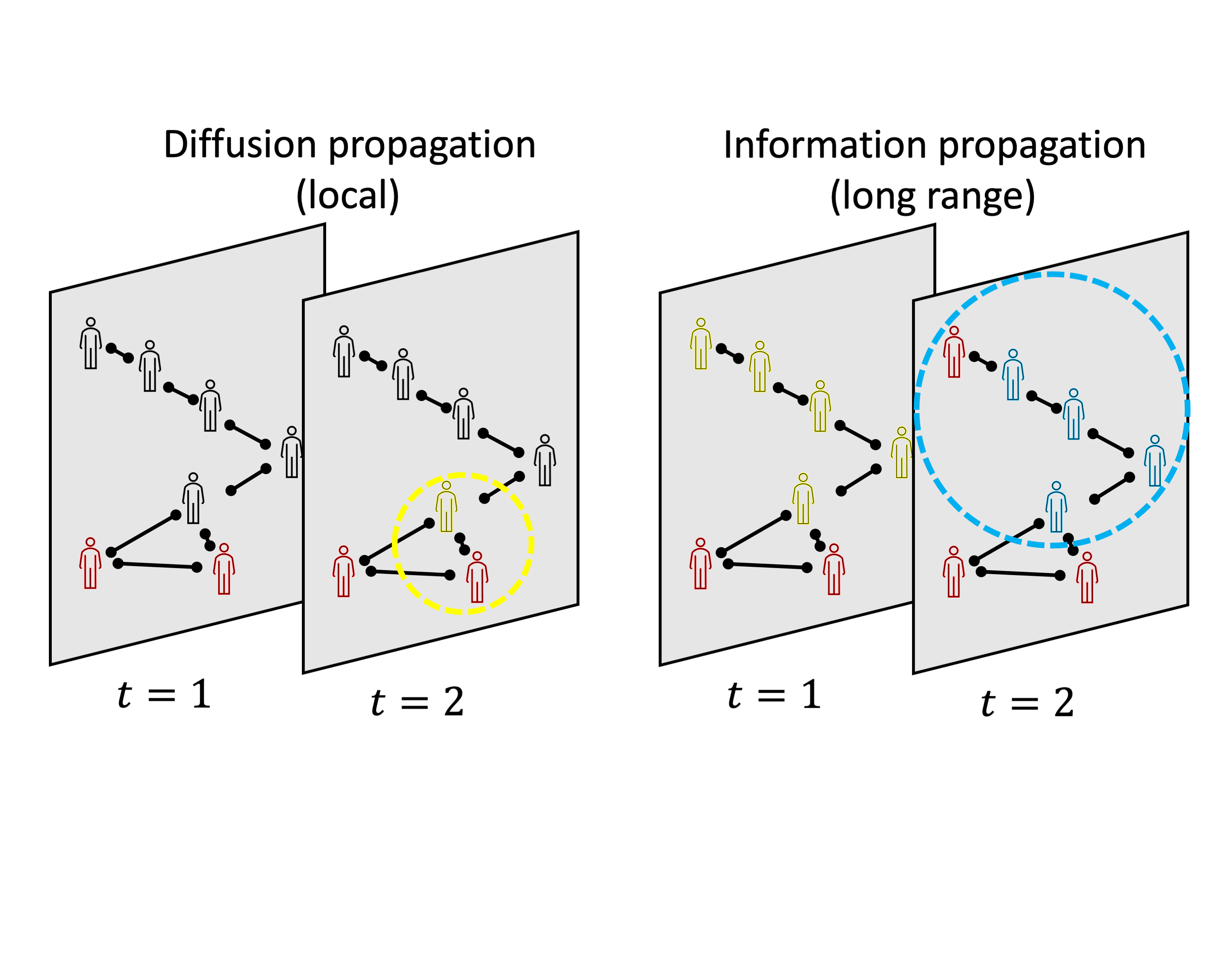
The main challenge in our setup is that the underlying dynamics is not directly and fully observed. Instead, partial information about the state of some nodes is given at each point in time. While the diffusive process spreads by point contacts, new node information may impact our belief on the state of a node a few hops away from the source of new information. For example, consider an epidemic spreading on a network. Detecting an infected person directly modifies the probability that nodes that are connected to it by a path in the temporal graph are also infected (Fig. 2). To address this issue, our architecture contains two separate GNN modules, one updates the node representation according to the dynamic process and the other is in charge of long range information propagation. These GNNs take as input a multi-graph over the nodes, where edges are time-stamped with the time of interactions. In addition, we show that combining RL with temporal graphs requires stabilizing information aggregation from other neighbors when updating nodes hidden states, and control how actions are sampled during training to ensure sufficient exploration. We show empirically the benefits of these components.
We test our approach on two very different problems, Influence Maximization and Epidemic Test Prioritization, and show that our approach outperforms state-of-the-art methods, often significantly. Our framework can be possibly further extended for problems beyond the ones mentioned here, e.g. traffic control, active sensing for complex scenes, etc.
This paper makes the following contributions: (1) A new RL framework for controlling partially-observed diffusive processes over graphs. We present a novel formulation of two challenging problems: the testing allocation problem and the partially-observed influence maximization problem. (2) A new architecture for controlling the dynamics of diffusive processes over graphs. Our architecture prioritizes interventions on a temporal multi-graph by leveraging deep Graph Neural Networks (GNNs). (3) A set of benchmarks and strong baselines, including network-based real-world contact tracing statistical data for COVID-19. Our RL approach achieves superior performance over these datasets.
2 A motivating example
We begin with an example to illustrate the trade-offs of the problem (Figure 3). In this example, our goal is to minimize the number of infected nodes in a social interactions graph.
Given a list of time-stamped interactions between nodes, we form a discrete time-varying graph as follows. If and interact at time , then the edge exists at time . Each interaction is characterized by a transmission probability , meaning that a healthy node that interacts with an infected node at time becomes infected with probability .
For the purpose of this example, assume that we can test a single node only at odd timesteps. If the node is positively tested as infected, it is quarantined and cannot further interact with other nodes. Otherwise, we do not perturb the dynamics and it may interact freely with its neighbors.
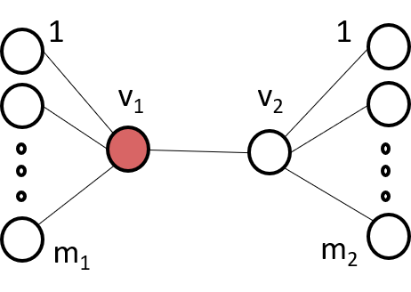
Consider the ”two stars” network in Figure 3. The left hub (node ) has neighbors, and the right hub () has . At only the edge is present with transmission probability . For all , all edges depicted in Figure 3 exist with transmission probability . Assume that this is known to the agent, and that at we suspect that was infected at . Clearly, we should either test or . It is easy to compute the expected number of infected nodes in both cases (details in Appendix A). The decision would be to test if and otherwise test .
This example illustrates that an optimal policy must balance two factors: the probability that the dynamics is affected - that a test action yields a “positive”, and the future consequences of our action - the strategic importance of selecting vs. , expressed by the ratio . A policy targeting likely-infected nodes will always pick node , but since it only focuses on the first term and ignores the second term, it is clearly suboptimal.
3 Problem Formulation
We start with a general formulation of the control problem, and then give two concrete examples from different domains: Epidemic test prioritization, and dynamic influence maximization. Formal definitions are given in Appendix B.
3.1 General formalism
Consider a graph whose structure changes in time. is the set of nodes and is the set of edges at step . Each edge is associated with features which may vary in time, and each node is characterized with features .
The state of a node is a random variable which can have values in . The node’s state dynamic depends on the interactions between and its neighbors, its state and the state of those neighbors, all at time . At each step, the agent selects a subset of nodes, and attempt to change the state of any selected node , namely, apply a stochastic transformation on a subset of the nodes. Selecting nodes and setting their states defines the action for the agent, and plays the role of a knob for controlling the global dynamics of the process over the graph. The action space consists of all possible selections of a subset of nodes . Even for moderate graph, with and small the action space is huge.
The optimization criterion depends only on the total number of nodes in state , . The objective is therefore of the form , where future evaluations are weighted by a discount factor . Additionally, the agent may be subject to constraints written in a similar manner .
3.2 Epidemic test prioritization
We consider the recent COVID-19 outbreak that spreads through social contacts. The temporal graph is defined over a group of nodes (people) , and its edges are determined by their daily social interactions. An edge between two nodes exists at time iff the two nodes interacted at time . Each of these interactions is characterized by features , including its duration, distancing and environment (e.g., indoors or outdoors). Additionally, each node has features (e.g., age, sex etc.).
The SEIR model dynamics (Lopez & Rodo, 2020). Every node (person) can be in one of the following states: susceptible – a healthy, yet uninfected person ( state), exposed/latent – infected but cannot infect others ( state), infectious – may infect other nodes ( state), or removed – self-quarantined and isolated from the graph ( state).
A healthy node can become infected by interacting with its neighbors. The testing intervention changes the state of a node. If infected or exposed, its state is set to , otherwise it remains as it is. More details can be found in the appendix.
Optimization goal, action space. The objective is to minimize the spread of the epidemic, namely, minimize the number of infected people (in either or states), over time. Our setup differs from previous work (e.g., (Hoffmann et al., 2020; Wang et al., 2020)) in two important aspects. First, we do not assume a node can be vaccinated or immunized against the epidemic. Second, we do not assume a node can be quarantined or disconnected from the graph without justification, namely, without a positive test result. Often, nodes perform required social functionality. Isolating a high-degree node from the network, like putting a bus-driver in quarantine, will either deteriorate the transportation network quality, or will require using a replacement driver that will have the same interactions pattern. A preemptive node removal would either not affect the network connectivity or impair the network functionality.
Observation space. At each time , the agent is exposed to all past interactions between network nodes, . In addition, we are given partial information on the nodes state. The agent is provided with information on a subset of the infectious nodes at . At every , the agent observes all past test results, i.e, for every we observe if node was healthy at or not.
3.3 Dynamic influence maximization
The classical multi-round influence maximization problem (Domingos & Richardson, 2001; Kempe et al., 2003; Lei et al., 2015) assumes the agent knows the groundtruth state of every node at every turn. More often than not, that is an unrealistic assumption. The agent can only know if a person is influenced if the person actively signals it, for example by using a coupon code. Furthermore, there might be a substantial delay from the time the information was presented to the time a feedback was received. Therefore, we extend this setup to include partial observability.
Model Dynamics. Each node is either Influenced or Susceptible. Influenced nodes try to influence their neighbors, following a dynamic generalization of two canonical models: Linear Threshold (LT) and Independent Cascades (IC). In an IC model, if is Influenced and , then may influence according to a probabilistic model. In a LT model, each node is associated with a threshold , and each edge carries an impact weight of . If the sum of edge weights, the cumulative ”peer pressure”, of neighboring infected nodes exceeds , node is influenced. See Appendix B for details on these models.
Optimization goal, action space. The goal is to maximize the number of Influenced nodes. All nodes start at the Susceptible state. At each step the agent selects a seed set of nodes, and attempts to influence them. Each attempt succeeds with some probability independently for every .
Observation space. At every step, an influenced node may reveal that it is influenced, e.g. by clicking on ads, with some probability . The set of these signals at previous times along with past interactions between nodes consists the observation space.
4 Approach
This section introduces our main contribution. Our goal is to select a subset of nodes for influencing the dynamics. The direct approach would be to perform a Monte Carlo simulation of the diffusive process for every possible action at every step, and choose the best performing action. However, this approach does not scale, and is unfeasible even for moderate networks (see Liu et al., 2017; Banerjee et al., 2020, and Appendix C for discussion). An alternative popular approach uses predefined heuristics or greedy approaches (e.g., (Yang et al., 2020; Preciado et al., 2014; Murata & Koga, 2018)), but this is arbitrary and often sub-optimal.
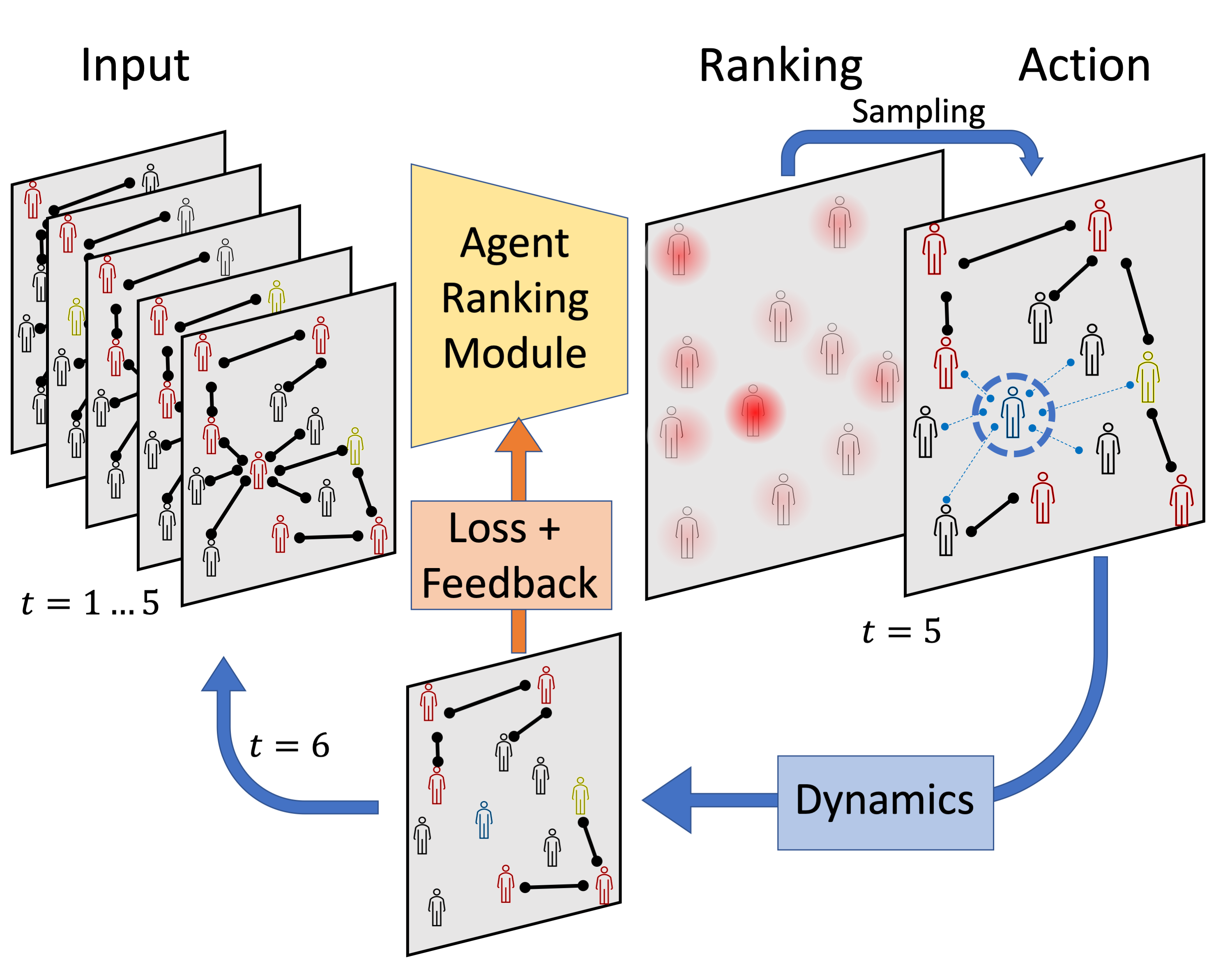
We propose a learning-based approach, which generalizes from past patterns collected during training. Since our goal is to maximize an objective over time in a dynamic environment, RL is a natural choice (Figure 4).
Yet, even with a learning approach, solving the general case of the subset selection problem would be combinatorially hard (Kempe et al., 2003) and is difficult to scale to large graphs. At the other extreme, a simple approximated solution can be achieved by scoring each node independently and then selecting the top-ranked nodes. Unfortunately, this approximation would potentially be far from optimal because it neglects correlations across nodes that are crucial. Therefore, it is important that node selection would consider other nodes, at least locally. For example, creating tight clusters of Influenced nodes is critical in Influence Maximization under the Linear Threshold model (see Appendix B). Assume that the intervention budget is sufficient for establishing a single cluster but there exist two equally beneficial regions to promote such cluster. The agent should learn to focus on one region rather than spread on two regions. This requires learning to choose optimal subsets rather than choosing nodes independently.
Our approach takes a mid-road: We use a graph neural network to compute per-node scores, where each node is exposed to the features of nodes in its extended -hop neighborhood (where is the depth of the GNN). This way, agent can learn to take into account complex correlations, and to select high-quality subsets by ranking nodes by their scores.
4.1 The Ranking Module
Overview.
In our approach, an RL agent receives as input the node and edge features of the temporal graph, and scores each node. The module that performs that scoring is called the ranking module (Figure 5). Scores are used to generate a probability distribution over nodes, and then for sampling a subset of nodes for testing. Namely, the scores encode the agent policy. The ranking module also updates the internal representation of each node, which aggregates past observations and information.
The score of a node is affected both by propagation dynamics and by information available to the agent. One may hope that on a short time scale the node score would only be affected by its neighboring nodes. Unfortunately, information can propagate long distances in the graph almost instantaneously, because revealing the state of one node in a long chain affects other nodes.To handle this effect, the ranking module contains two GNNs (see Fig. 5). (1) A local diffusion component updates the diffusion process state; and (2) a long-range information component updates the information state.
We use Proximal Policy Optimization (PPO) (Schulman et al., 2017) to optimize our agent. We sequentially apply the suggested action, log the (state, action) tuple in an experience replay buffer, and train our model based on the PPO loss term. We further motivate our framework and extended the discussion on our design choices in Appendix C.
4.2 Modules
Input. The input to the ranking module consists of three feature types: (1) Static node features : e.g., topological graph centralities (betweenness, closeness, eigenvector, and degree centralities) and random node features. (2) Dynamic node features : All intervention results up to the current timestamp. We denote all nodes features as a concatenation . (3) Edge features and the structure of the temporal graph : All previous interactions up to the current step, including the transmission probability for each interaction. All these features are scalars, except the dynamic node features, which are encoded as one hot vectors. Figure 5 illustrates the basic data flow in the ranking module.
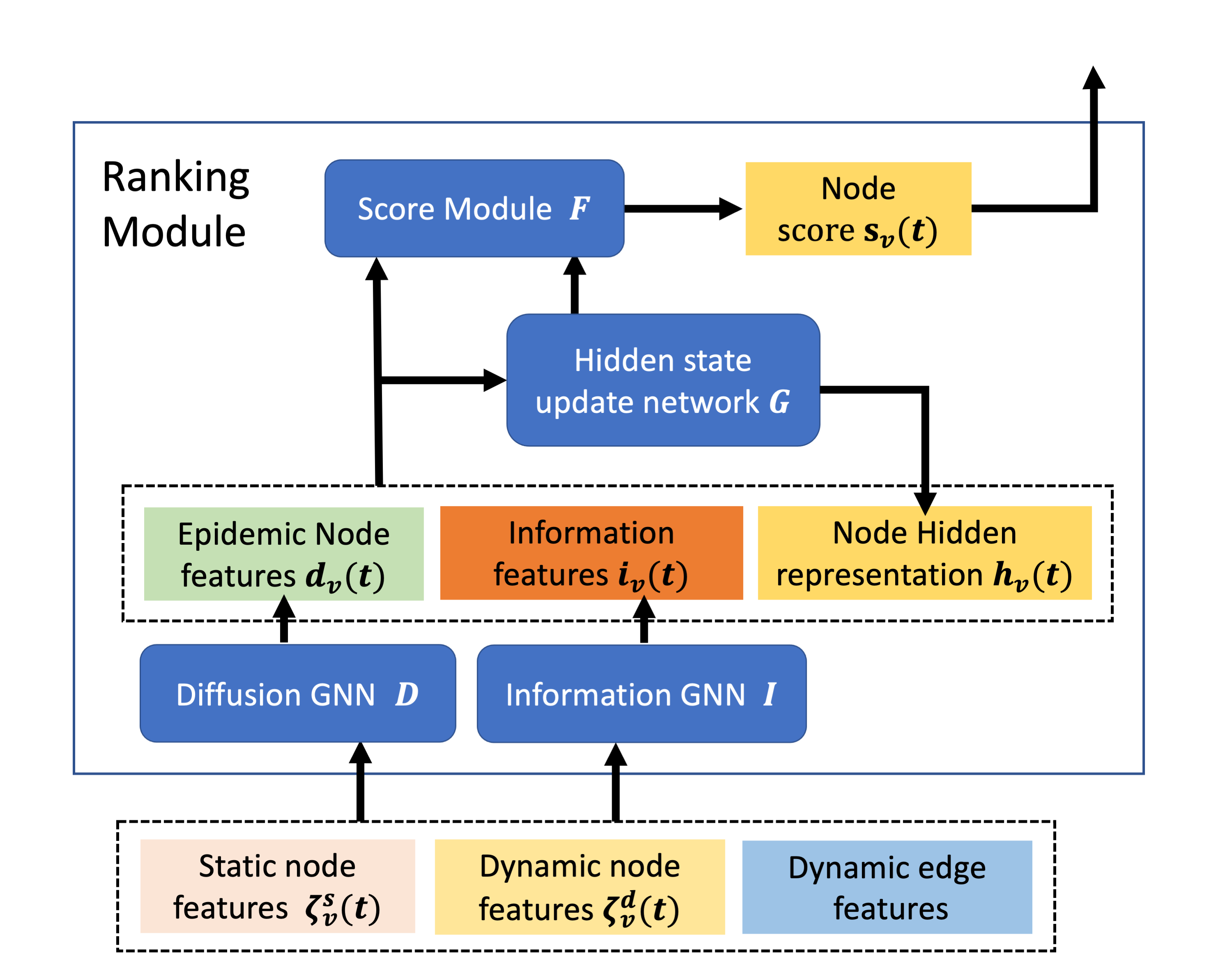
Local diffusion GNN. The spread through point contact is modeled by a GNN . As the diffusive process spreads by only one hop per step, it is sufficient to model the spread with a single GNN layer. Formally, denote by an interaction between and at time , and by the probability of transmission during this interaction. For each , the output of is a feature vector denoted by :
where is multilayer perceptron (MLP). Rather than considering the probability as an edge feature, this component mimics the dynamic process transition rule to accelerate learning.
Long-range information GNN. GNN computes the information state of each node. As discussed above, updated information on a node a few hops away from node may abruptly change our belief on the state of . Furthermore, this change may occur even if and did not interact in the last time step but rather a while ago. To update the information state, we construct a cumulative multi-graph where the set of edges between nodes and at time are all the interactions that occurred during the last steps. The features of each edge at time are the interaction delay and the transmission probability . The information features are the output of -layer GNN; the layer is:
As before, is an MLP, with and are the final node features.
Score and hidden state update. For every node we hold a hidden state , updated according to a neural network ,
| (1) |
After updating the new node hidden states, we use them to calculate the node scores using a neural network ,
| (2) |
Here, and are two additional components (see Fig. 5). is an MLP, while can be either an MLP or recurrent module such as GRU.
4.3 Sampling and scoring
During inference, we pick the top scored nodes. During training, to encourage exploration we use the score per node to sample nodes. We (1) map the score of nodes to a probability distribution (2) sample a node, and (3) adjust the distribution by removing its weight. We repeat this process iterations (sample without replacement).
Score-to-probability. Usually, node scores are converted to a distribution over actions using a softmax. As demonstrated in (Mei et al., 2020), this approach is problematic as node probabilities decay exponentially with their scores, leading to two major drawbacks: it discourages exploration of low-score nodes, and also limits sensitivity to the top of the distribution rather than at the -th ranked node. Instead, we set the probability to sample an action to
| (3) |
where is the set of scores and a constant. The probability difference between low scoring nodes and high scoring nodes becomes less extreme than softmax. Furthermore, the parameter controls the initial exploration ratio. We compare our approach with the recent escort transform (Mei et al., 2020) that is considered to be a state-of-the-art score-to-probability method. As shown in Appendix D, our method outperforms the escort transform in this problem.
5 Experiments
We evaluated our approach in two tasks: (1) Epidemic test prioritization, and (2) Dynamic influence maximization. More experiments and details are in Appendix D.
Real-World Datasets. We tested our algorithm and baselines on graphs of different sizes and sources, ranging from 5K to over 100K nodes. (1) CA-GrQcA A research collaboration network (Rossi & Ahmed, 2015). (2) Montreal, based on WiFi hotspot tracing(Hoen et al., 2015). (3) Portland: a compartment-based synthetic network (Wells et al., 2013; Eubank et al., 2004). (4) Email: An email network (Leskovec et al., 2007) (5) GEMSEC-RO: (Rozemberczki et al., 2019), friendship relations in the Deezer music service. All these networks have been extensively used in previous works, in particular in epidemiological studies, as key networks models (Sambaturu et al., 2020; Yang et al., 2020; Herrera et al., 2016; Wells et al., 2013; Eubank et al., 2004). Table S4 summarizes the datasets.
Synthetic Datasets. We considered three synthetic, random network families: (1) Community-based networks have nodes clustered into densely-connected communities, with sparse connections across communities. We use the Stochastic Block Model (SBM, (Abbe, 2017)), for 2 and 3 communities. (2) Preferential attachment (PA) networks exhibit a node-degree distribution that follows a power-law (scale-free), like those found in many real-world networks. We used the dual Barbarsi-Albert model (Moshiri, 2018). (3) Contact-tracing networks. We received anonymized high-level statistical information (see Appendix D) about real contact tracing networks, collected during April 2020.
Generating temporal graphs. For all networks except CT graphs, at each time step we select uniformly at random a subset of edges and then assign to each edge a transmission probability sampled uniformly in . We use a different methodology for the CT graphs, See Appendix D for details.
Training procedure. Algorithms were trained on randomly generated PA networks with nodes. Each experiment was performed with at least three random seeds.
5.1 Epidemic test prioritization
5.1.1 Baselines
We compare methods from three categories.
A. Preprogrammed heuristic (no-learning) baselines. Rank nodes based on: (1) Infected neighborhood: Number of known infected nodes in their 2-hop neighborhood (Meirom et al., 2015, 2018). (2) Probabilistic risk: Probability of infection at time . Using dynamic programming to analytically solve the probability propagation. (3) Degree centrality (Salathé & Jones, 2010; Sambaturu et al., 2020). (4) Eigenvector centrality: (Preciado et al., 2014; Yang et al., 2020).
B. Supervised learning. Learn the risk per-node using features of the temporal graph, its connectivity, and infection state. Each time step and node is a sample, and its label is determined by the next step. (5) Supervised (vanilla). Features include a static component described in Section 4.1, and a dynamic part that contains the number of infected neighbors and their neighbors. (6) Supervised (+GNN). Like #5, the input is the set of all historic interactions of ’s and its -order neighbors.(7) Supervised (+weighted degree). Like #6, the loss weighs nodes are by their degree. (8) Supervised (+weighted degree +GNN). Like #6 above, using degree-weighted loss like #7.
C. RL algorithms: RLGN is our algorithm described in Section 4. The input to (9) RL-vanilla is the same as in (#1) and (#6) above. Correspondingly, the GNN module described in Section 4 is replaced by a DNN similar to (#6).
Evaluation Metric. The end goal of quarantining and epidemiological testing is to minimize the spread of the epidemic. Our success metric is therefore the percent of nodes kept healthy throughout the simulation. An auxiliary metric we sometime used was %contained: The probability of containing the epidemic. This was computed as the fraction of simulations having cumulative infected nodes smaller than a fraction .
5.1.2 Results
In the first set of experiments, we compared RLGN with the 9 baselines described in Section 5.1.1 on the synthetic networks described above. The results reported in Table 1 show that RLGN outperforms all baselines on all network types. We selected the top-performing algorithms and evaluated them on the large, real-world networks dataset.
| PA | CT | |
| Tree-based (2) | ||
| Counter model (1) | ||
| Degree (3) | ||
| Eigenvector (4) | ||
| SL (vanilla) (5) | ||
| SL + GNN (6) | 2 | |
| SL + deg (7) | ||
| SL + deg + GNN (8) | ||
| RL (vanilla) (9) | ||
| RLGN (ours) | 522 | 401 |
Table 2 compares the performance of the RLGN and the best baseline (SL) on the large-scale datasets. We included the centralities baselines (#3,#4) in the comparison as they are heavily used in epidemiological studies. Table 2 shows that RLGN consistently performs better than the baselines, and the gap is clearly statistically significant. We also evaluated the performance of RLGN on a Preferential Attachment network with nodes (mean degree ), as this random network model is considered a reasonable approximation for many other real-world networks. The mean percentile of healthy nodes at the end of the episode was for RLGN, while for the SL+GNN it was only , a difference of more than STDs.
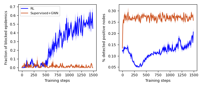
Analysis. To gain insight into these results, Figure 6 traces the fraction of contained epidemics and infected nodes during training in 3-community networks. Supervised learning detects substantially more infected nodes than RLGN (right panel), but these tend to have a lower future impact on the spread, and it fails to contain the epidemic (left). A closer look shows that RLGN, but not SL, successfully learns to identify and neutralize the critical nodes that connect communities and prevent the disease from spreading to another community. See a video highlighting these results online 111Link: https://youtu.be/Rhqy7YY9gX8.
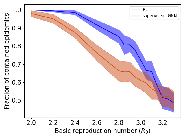
When would RLGN be successful? In sparsely connected networks, it is easy to cut long infection chains, and both approaches succeed. In densely connected networks, there are no critical nodes, because there are many paths between any two nodes. This can also be viewed in terms of the coefficient, the mean number of nodes infected by a single diseased node. The greater , the more difficult it is to contain the epidemic. Therefore, we expect RLGN to excel in intermediate regimes. Fig. S1(a) indeed shows that RL has a significant advantage over supervised+GNN for a range of values between and .
We have deepened our analysis, and investigated: (1) Can we quantify the algorithm by their ability to reduce , the mean number of nodes infected by a single diseased node? Can we quantify the performance by the number of tests required to achieve the same level of performance, measuring their effective test utilization? (2) How robust the trained algorithms to variations in the epidemiological parameters? (3) How does the performance gap between the algorithms scale with the network size? Due to lack of space, we expand on these topics in Appendix D.
Appendix D also includes a comparison between RLGN and the best performing baselines across a range of network sizes, initial infection sizes and testing capacities (Table S6).
Ablation studies. We assess the importance of key elements in our framework using ablation studies. First, to quantify the contribution of the information module, we removed it completely from our DNN module, keeping only the epidemic module. The full DNN module achieved a contained epidemic score of , while the ablated DNN module corresponding score was , a degradation of more than . This shows that the information module has a critical role in improving the performance of the RLGN framework.
Second, in the opposite direction, one may wonder: Why separate local and long-range GNNs, rather than a single higher-capacity network? We found that using a local-diffusion GNN training converges faster (Fig. S3). Presumably, because it models the process more closely to the true spreading.
Appendix D contains additional ablation studies of key elements in our framework: (A) Our score-to-probability function outperforms the popular softmax distribution and escort transform. (B) Internal state normalization in scale-free networks accelerates training substantially.
| CA-GrQc | Montreal | Portland | Enron | GEMSEC-RO | |
| Degree | |||||
| E.vector | |||||
| SL | |||||
| RLGN | 42.7 | 39.7 | 3.71 | 89.2 | 6.5 |
5.2 Influence Maximization
| CA-GrQc | Montreal | Enron | GEMSEC-RO | CA-HEPTh | |
|---|---|---|---|---|---|
| LIR (Liu et al., 2017) | |||||
| LIR (filtered) | |||||
| Degree | |||||
| Degree Discounted (Murata & Koga, 2018) | |||||
| Eigenvector (Bozorgi et al., 2016) | |||||
| RLGN (ours) |
Baselines. Unlike the epidemic test prioritization, in this problem there is no supervised signal; there is no immediate feedback that may be used for supervision. We compare our RLGN framework against the state-of-the-art scalable algorithms. (1) LIR (Liu et al., 2017) is an algorithm for top-k ranking for the IM problem. It was shown to achieve similar performance to MC based methods. (2) LIR (filtered): LIR was designed for a fully observable setup. We extend this algorithm to a partially observed setup and filter out nodes with an identified influenced neighbor. The motivation is that it is likely that such nodes are already influenced or likely to be influenced soon. (3) Degree discounted (Chen et al., 2009) is a topology-based algorithm that was shown to achieve a state-of-the-art performance on some networks, and was recently extended to temporal graphs (Murata & Koga, 2018). (4) Degree Centrality and (5) Eigenvector Centrality, defined previously, were also used extensively (Lei et al., 2015; Chen et al., 2014; Bozorgi et al., 2016).
Results. We have compared RLGN against the aforementioned baselines on the real-world datasets in Table 3. We included an additional (CA-HEPTh) network that was frequently used as a benchmark for this problem.
6 Previous work
Deep Learning on graphs. Graph neural networks (GNNs) are deep neural networks that can process graph-structured data (Sperduti, 1993, 1994; Sperduti & Starita, 1997; Pollack, 1990; Küchler & Goller, 1996; Kipf & Welling, 2016; Gilmer et al., 2017; Duvenaud et al., 2015; Hamilton et al., 2017; Veličković et al., 2017). Several works combine recurrent mechanisms with GNNs to learn temporal graph data, (Liu et al., 2019; Rossi et al., 2020; Liu & Zhou, 2020; Pareja et al., 2019). Further information can be found in (Kazemi et al., 2020).
Ranking on graphs. The problem of ranking on graphs is a fundamental CS problem. It has various applications such as web page ranking (Page et al., 1999; Agarwal, 2006) and knowledge graph search (Xiong et al., 2017).
Reinforcement learning and graphs studies can be split into two main categories: leveraging graph structure for general RL problems (Zhang et al., 2018a; Jiang et al., 2018), and applying RL methods for graph problems. Our work falls into the latter. An important line of work uses RL to solve NP-hard combinatorial optimization problems on graphs. (Zhu et al., 2019; Dai et al., 2017; Wei et al., 2021).
Manipulation of dynamic processes on graphs. The problem of node manipulation (e.g., vaccination) for controlling epidemic processes on graphs was intensively studied (Hoffmann et al., 2020; Medlock & Galvani, 2009). This problem is often addressed in the setup of the fire-fighter problem and its extensions (Finbow & Macgillivray, 2009; Tennenholtz et al., 2017; Sambaturu et al., 2020). Other work considered the problem of vaccination assignments, and cast this problem into a minimal cover problem (Wang et al., 2020; Song et al., 2020; Wijayanto & Murata, 2019). Other common approaches include developing centrality measures designed to highlight bottleneck nodes (Yang et al., 2020), or using spectral methods for allocating resources (Saha et al., 2015; Preciado et al., 2014; Ogura & Preciado, 2017). Alternative line of research (Miller & Hyman, 2007; Cohen et al., 2002) developed heuristics for the same task.
In most previous work setups a single decision is taken. In our multi-round setup, the agent performs a sequential decision making. The agent needs to balance between retrieving information (for better informed future decisions), maximizing the probability that the intervention will be successful, and optimizing the long-term goal.
Influence Maximization, (IM) is a canonical optimization problem of dynamical processes on graphs. IM was first presented in (Kempe et al., 2003), and proved to be NP-Hard and hard to approximate. Key approximation algorithms were derived in (Goyal et al., 2011; Nguyen et al., 2016), but since they do not scale to large graphs, many alternative heuristics were developed (Murata & Koga, 2018; Liu et al., 2017). For surveys, see Banerjee et al. (2020); Li et al. (2018). Multi-armed Bandit was used for estimating model parameters (Vaswani et al., 2017; Lei et al., 2015). The IM formulation was extended to a multi-round framework by Lin et al. (2015). Chung et al. (2019); Tian et al. (2020); Lin et al. (2015) used RL to find the optimal combination of heuristics from a short list of hand-designed features.
These approaches are limited by the small number of pre-selected heuristics and by the problem-specific, hand-crafted features. In contrast, our approaches is general and it is not limited to reweighting or a predefined subset of policies, neither uses hand-designed, problem-specific features. Our agent learns a policy from scratch and uses GNNs to generalize to different domains (Yehudai et al., 2021).
7 Conclusions
This paper shows that combining RL with GNNs provides a powerful approach for controlling diffusive processes on graphs. Our approach handles an exponential state space, combinatorial action space and partial observability, and achieves superior performance on challenging tasks on large, real-world networks.
The approach and model discussed in this paper can be applied to important problems other than epidemic control and influence maximization. For example, fake news can be maliciously distributed, and spread over the network. A decision maker can verify the authenticity of items, but only verify a limited number of items per a time period. The objective would be to minimize the total number of nodes that observe fake items.
Our approach assumes that a decision taken by considering only hops neighborhood of each node is a fairly good approximation to the optimal policy which takes into account the whole graph. If long range correlations exists, this may deteriorate performance. As such, it is sufficient to train our model on small graphs and infer on a larger graph. An interesting question is the ability of our approach to address edge cases that may result from this training protocol, and the generalization ability of our model as a function of long-range correlations in the data.
A key concern for real world application is privacy preservation of individual nodes. Our approach requires local aggregated information about the node’s neighborhood, compared to other approaches (e.g., (Kempe et al., 2003; Yang et al., 2020) which required detailed information on the complete graph. Furthermore, recent papers (Zhou et al., 2021) have shown that it is possible to use graph neural network while preserving privacy, and we leave it for future research to apply such approaches in this setup.
References
- Abbe (2017) Abbe, E. Community detection and stochastic block models: recent developments. The Journal of Machine Learning Research, 18(1):6446–6531, 2017.
- Agarwal (2006) Agarwal, S. Ranking on graph data. In Proceedings of the 23rd international conference on Machine learning, pp. 25–32, 2006.
- Banerjee et al. (2020) Banerjee, S., Jenamani, M., and Pratihar, D. K. A survey on influence maximization in a social network. Knowledge and Information Systems, 62(9):3417–3455, sep 2020. ISSN 02193116. doi: 10.1007/s10115-020-01461-4. URL https://link.springer.com/article/10.1007/s10115-020-01461-4.
- Barabási (1999) Barabási, A. Emergence of Scaling in Random Networks. Science, 286(5439):509–512, oct 1999. ISSN 00368075. doi: 10.1126/science.286.5439.509. URL http://www.sciencemag.org/content/286/5439/509.abstract.
- Bozorgi et al. (2016) Bozorgi, A., Haghighi, H., Sadegh Zahedi, M., and Rezvani, M. INCIM: A community-based algorithm for influence maximization problem under the linear threshold model. Information Processing and Management, 52(6):1188–1199, nov 2016. ISSN 03064573. doi: 10.1016/j.ipm.2016.05.006.
- Chen et al. (2009) Chen, W., Wang, Y., and Yang, S. Efficient influence maximization in social networks. In Proceedings of the ACM SIGKDD International Conference on Knowledge Discovery and Data Mining, pp. 199–207, New York, New York, USA, 2009. ACM Press. ISBN 9781605584959. doi: 10.1145/1557019.1557047. URL http://portal.acm.org/citation.cfm?doid=1557019.1557047.
- Chen et al. (2014) Chen, Y. C., Zhu, W. Y., Peng, W. C., Lee, W. C., and Lee, S. Y. CIM: Community-based influence maximization in social networks. ACM Transactions on Intelligent Systems and Technology, 5(2):1–31, apr 2014. ISSN 21576912. doi: 10.1145/2532549. URL https://dl.acm.org/doi/10.1145/2532549.
- Chung et al. (2019) Chung, T.-Y., Citi, A. S., Taipei, T., Khurshed, A., Wang, C.-Y., and Ali, K. Deep Reinforcement Learning-based Approach to Tackle Competitive Influence Maximization. Technical report, 2019. URL https://doi.org/10.475/123{_}4.
- Cohen et al. (2002) Cohen, R., Havlin, S., and Ben-Avraham, D. Efficient Immunization Strategies for Computer Networks and Populations. Physical Review Letters, 91(24), jul 2002. doi: 10.1103/PhysRevLett.91.247901. URL http://arxiv.org/abs/cond-mat/0207387http://dx.doi.org/10.1103/PhysRevLett.91.247901.
- Dai et al. (2017) Dai, H., Khalil, E. B., Zhang, Y., Dilkina, B., and Song, L. Learning Combinatorial Optimization Algorithms over Graphs. Advances in Neural Information Processing Systems, 2017-Decem:6349–6359, apr 2017. URL http://arxiv.org/abs/1704.01665.
- Domingos & Richardson (2001) Domingos, P. and Richardson, M. Mining the network value of customers. In Proceedings of the seventh ACM SIGKDD international conference on Knowledge discovery and data mining, pp. 57–66, 2001.
- Duvenaud et al. (2015) Duvenaud, D. K., Maclaurin, D., Iparraguirre, J., Bombarell, R., Hirzel, T., Aspuru-Guzik, A., and Adams, R. P. Convolutional networks on graphs for learning molecular fingerprints. In Advances in neural information processing systems, pp. 2224–2232, 2015.
- Eubank et al. (2004) Eubank, S., Guclu, H., Kumar, V. S., Marathe, M. V., Srinivasan, A., Toroczkai, Z., and Wang, N. Modelling disease outbreaks in realistic urban social networks. Nature, 429(6988):180–184, may 2004. ISSN 00280836. doi: 10.1038/nature02541. URL www.nature.com/nature.
- Fey & Lenssen (2019) Fey, M. and Lenssen, J. E. Fast graph representation learning with pytorch geometric. arXiv preprint arXiv:1903.02428, 2019.
- Finbow & Macgillivray (2009) Finbow, S. and Macgillivray, G. The Firefighter Problem: A survey of results, directions and questions. The Australasian Journal of Combinatorics [electronic only], 43, 2009.
- Gilmer et al. (2017) Gilmer, J., Schoenholz, S. S., Riley, P. F., Vinyals, O., and Dahl, G. E. Neural message passing for quantum chemistry. In International Conference on Machine Learning, pp. 1263–1272, 2017.
- Goyal et al. (2011) Goyal, A., Lu, W., and Lakshmanan, L. V. CELF++: Optimizing the greedy algorithm for influence maximization in social networks. In Proceedings of the 20th International Conference Companion on World Wide Web, WWW 2011, pp. 47–48, New York, New York, USA, 2011. ACM Press. ISBN 9781450305181. doi: 10.1145/1963192.1963217. URL http://portal.acm.org/citation.cfm?doid=1963192.1963217.
- Hamilton et al. (2017) Hamilton, W. L., Ying, R., and Leskovec, J. Inductive Representation Learning on Large Graphs. Advances in Neural Information Processing Systems, 2017-Decem:1025–1035, jun 2017. URL http://arxiv.org/abs/1706.02216.
- Herrera et al. (2016) Herrera, J. L., Srinivasan, R., Brownstein, J. S., Galvani, A. P., and Meyers, L. A. Disease Surveillance on Complex Social Networks. PLOS Computational Biology, 12(7):e1004928, jul 2016. ISSN 1553-7358. doi: 10.1371/journal.pcbi.1004928. URL https://dx.plos.org/10.1371/journal.pcbi.1004928.
- Hoen et al. (2015) Hoen, A. G., Hladish, T. J., Eggo, R. M., Lenczner, M., Brownstein, J. S., and Meyers, L. A. Epidemic wave dynamics attributable to urban community structure: A theoretical characterization of disease transmission in a large network. Journal of Medical Internet Research, 17(7):e169, jul 2015. ISSN 14388871. doi: 10.2196/jmir.3720. URL https://www.jmir.org/2015/7/e169/.
- Hoffmann et al. (2020) Hoffmann, J., Jordan, M., and Caramanis, C. Quarantines as a Targeted Immunization Strategy. aug 2020. URL http://arxiv.org/abs/2008.08262.
- Jiang et al. (2018) Jiang, J., Dun, C., Huang, T., and Lu, Z. Graph Convolutional Reinforcement Learning. oct 2018. URL http://arxiv.org/abs/1810.09202.
- Kazemi et al. (2020) Kazemi, S. M., Goel, R., Jain, K., Kobyzev, I., Sethi, A., Forsyth, P., and Poupart, P. Representation learning for dynamic graphs: A survey. Journal of Machine Learning Research, 21(70):1–73, 2020.
- Kempe et al. (2003) Kempe, D., Kleinberg, J., and Tardos, É. Maximizing the spread of influence through a social network. In Proceedings of the ACM SIGKDD International Conference on Knowledge Discovery and Data Mining, pp. 137–146, New York, New York, USA, 2003. ACM Press. doi: 10.1145/956750.956769. URL http://portal.acm.org/citation.cfm?doid=956750.956769.
- Kipf & Welling (2016) Kipf, T. N. and Welling, M. Semi-supervised classification with graph convolutional networks. arXiv preprint arXiv:1609.02907, 2016.
- Küchler & Goller (1996) Küchler, A. and Goller, C. Inductive learning in symbolic domains using structure-driven recurrent neural networks. In Lecture Notes in Computer Science (including subseries Lecture Notes in Artificial Intelligence and Lecture Notes in Bioinformatics), volume 1137, pp. 183–197. Springer Verlag, 1996. ISBN 3540617086. doi: 10.1007/3-540-61708-6˙60. URL https://link.springer.com/chapter/10.1007/3-540-61708-6{_}60.
- Lei et al. (2015) Lei, S., Maniu, S., Mo, L., Cheng, R., and Senellart, P. Online influence maximization. In Proceedings of the ACM SIGKDD International Conference on Knowledge Discovery and Data Mining, volume 2015-August, pp. 645–654, New York, NY, USA, aug 2015. Association for Computing Machinery. ISBN 9781450336642. doi: 10.1145/2783258.2783271. URL https://dl.acm.org/doi/10.1145/2783258.2783271.
- Leskovec et al. (2007) Leskovec, J., Kleinberg, J., and Faloutsos, C. Graph evolution. ACM Transactions on Knowledge Discovery from Data, 1(1):2–es, mar 2007. ISSN 15564681. doi: 10.1145/1217299.1217301. URL http://dl.acm.org/citation.cfm?id=1217299.1217301.
- Li et al. (2018) Li, Y., Fan, J., Wang, Y., and Tan, K. L. Influence Maximization on Social Graphs: A Survey. IEEE Transactions on Knowledge and Data Engineering, 30(10):1852–1872, oct 2018. ISSN 15582191. doi: 10.1109/TKDE.2018.2807843.
- Lin et al. (2015) Lin, S. C., Lin, S. D., and Chen, M. S. A learning-based framework to handle multi-round multi-party influence maximization on social networks. In Proceedings of the ACM SIGKDD International Conference on Knowledge Discovery and Data Mining, volume 2015-Augus, pp. 695–704, New York, NY, USA, aug 2015. Association for Computing Machinery. ISBN 9781450336642. doi: 10.1145/2783258.2783392. URL https://dl.acm.org/doi/10.1145/2783258.2783392.
- Liu et al. (2017) Liu, D., Jing, Y., Zhao, J., Wang, W., and Song, G. A Fast and Efficient Algorithm for Mining Top-k Nodes in Complex Networks. Scientific Reports, 7(1):1–8, feb 2017. ISSN 20452322. doi: 10.1038/srep43330. URL www.nature.com/scientificreports.
- Liu & Zhou (2020) Liu, Z. and Zhou, D. Towards fine-grained temporal network representation via time-reinforced random walk. In Proceedings of the AAAI Conference on Artificial Intelligence, 2020.
- Liu et al. (2019) Liu, Z., Zhou, D., and He, J. Towards explainable representation of time-evolving graphs via spatial-temporal graph attention networks. In Proceedings of the 28th ACM International Conference on Information and Knowledge Management, pp. 2137–2140, 2019.
- Lopez & Rodo (2020) Lopez, L. and Rodo, X. A Modified SEIR Model to Predict the COVID-19 Outbreak in Spain and Italy: Simulating Control Scenarios and Multi-Scale Epidemics. SSRN Electronic Journal, pp. 2020.03.27.20045005, apr 2020. ISSN 1556-5068. doi: 10.1101/2020.03.27.20045005. URL https://doi.org/10.1101/2020.03.27.20045005.
- Medlock & Galvani (2009) Medlock, J. and Galvani, A. P. Optimizing influenza vaccine distribution. Science, 325(5948):1705–1708, sep 2009. ISSN 00368075. doi: 10.1126/science.1175570. URL https://science.sciencemag.org/content/325/5948/1705https://science.sciencemag.org/content/325/5948/1705.abstract.
- Mei et al. (2020) Mei, J., Xiao, C., Dai, B., Li, L., Szepesvári, C., and Schuurmans, D. Escaping the Gravitational Pull of Softmax. In Advances in Neural Information Processing Systems 33 (NeurIPS 2020), 2020.
- Meirom et al. (2015) Meirom, E. A., Milling, C., Caramanis, C., Mannor, S., Shakkottai, S., and Orda, A. Localized epidemic detection in networks with overwhelming noise. submitted to ACM SIGMETRICS 2015, 2015.
- Meirom et al. (2018) Meirom, E. A., Caramanis, C., Mannor, S., Orda, A., and Shakkottai, S. Detecting Cascades from Weak Signatures. IEEE Transactions on Network Science and Engineering, 5(4):313–325, oct 2018. ISSN 2334-329X. doi: 10.1109/TNSE.2017.2764444.
- Miller & Hyman (2007) Miller, J. C. and Hyman, J. M. Effective vaccination strategies for realistic social networks. Physica A: Statistical Mechanics and its Applications, 386(2):780–785, 2007. ISSN 0378-4371. doi: https://doi.org/10.1016/j.physa.2007.08.054. URL http://www.sciencedirect.com/science/article/pii/S037843710700948X.
- Moshiri (2018) Moshiri, N. The dual-Barabasi-Albert model. oct 2018. URL http://arxiv.org/abs/1810.10538.
- Murata & Koga (2018) Murata, T. and Koga, H. Extended methods for influence maximization in dynamic networks. Computational Social Networks, 5(1):8, dec 2018. ISSN 21974314. doi: 10.1186/s40649-018-0056-8. URL https://computationalsocialnetworks.springeropen.com/articles/10.1186/s40649-018-0056-8.
- Newman (2010) Newman, M. Networks: An Introduction. may 2010. URL http://dl.acm.org/citation.cfm?id=1809753.
- Nguyen et al. (2016) Nguyen, H. T., Thai, M. T., and Dinh, T. N. Stop-and-Stare: Optimal Sampling Algorithms for Viral Marketing in Billion-scale Networks. Proceedings of the ACM SIGMOD International Conference on Management of Data, 26-June-20:695–710, may 2016. URL http://arxiv.org/abs/1605.07990.
- Ogura & Preciado (2017) Ogura, M. and Preciado, V. M. Optimal Containment of Epidemics in Temporal and Adaptive Networks. pp. 241–266. Springer, Singapore, 2017. doi: 10.1007/978-981-10-5287-3˙11. URL https://link.springer.com/chapter/10.1007/978-981-10-5287-3{_}11.
- Page et al. (1999) Page, L., Brin, S., Motwani, R., and Winograd, T. The pagerank citation ranking: Bringing order to the web. Technical report, Stanford InfoLab, 1999.
- Pareja et al. (2019) Pareja, A., Domeniconi, G., Chen, J., Ma, T., Suzumura, T., Kanezashi, H., Kaler, T., Schardl, T. B., and Leiserson, C. E. EvolveGCN: Evolving Graph Convolutional Networks for Dynamic Graphs. feb 2019. URL http://arxiv.org/abs/1902.10191.
- Paszke et al. (2017) Paszke, A., Gross, S., Chintala, S., Chanan, G., Yang, E., DeVito, Z., Lin, Z., Desmaison, A., Antiga, L., and Lerer, A. Automatic differentiation in pytorch. 2017.
- Pollack (1990) Pollack, J. B. Recursive distributed representations. Artificial Intelligence, 46(1-2):77–105, nov 1990. ISSN 00043702. doi: 10.1016/0004-3702(90)90005-K.
- Preciado et al. (2014) Preciado, V. M., Zargham, M., Enyioha, C., Jadbabaie, A., and Pappas, G. J. Optimal resource allocation for network protection against spreading processes. IEEE Transactions on Control of Network Systems, 1(1):99–108, mar 2014. ISSN 23255870. doi: 10.1109/TCNS.2014.2310911.
- Rossi et al. (2020) Rossi, E., Chamberlain, B., Frasca, F., Eynard, D., Monti, F., and Bronstein, M. Temporal graph networks for deep learning on dynamic graphs. arXiv preprint arXiv:2006.10637, 2020.
- Rossi & Ahmed (2015) Rossi, R. A. and Ahmed, N. K. The Network Data Repository with Interactive Graph Analytics and Visualization. In AAAI, 2015. URL http://networkrepository.com.
- Rozemberczki et al. (2019) Rozemberczki, B., Davies, R., Sarkar, R., and Sutton, C. GEMSEC: Graph Embedding with Self Clustering. In Proceedings of the 2019 IEEE/ACM International Conference on Advances in Social Networks Analysis and Mining 2019, pp. 65–72. ACM, 2019.
- Saha et al. (2015) Saha, S., Adiga, A., Prakash, B. A., and Vullikanti, A. K. S. Approximation algorithms for reducing the spectral radius to control epidemic spread. In SIAM International Conference on Data Mining 2015, SDM 2015, pp. 568–576. Society for Industrial and Applied Mathematics Publications, 2015. ISBN 9781510811522. doi: 10.1137/1.9781611974010.64. URL https://epubs.siam.org/page/terms.
- Salathé & Jones (2010) Salathé, M. and Jones, J. H. Dynamics and control of diseases in networks with community structure. PLoS Computational Biology, 6(4), apr 2010. ISSN 1553734X. doi: 10.1371/journal.pcbi.1000736.
- Sambaturu et al. (2020) Sambaturu, P., Adhikari, B., Prakash, B. A., Venkatramanan, S., and Vullikanti, A. Designing Effective and Practical Interventions to Contain Epidemics. In Proceedings of the 19th International Conference on Autonomous Agents and MultiAgent Systems, AAMAS ’20, pp. 1187–1195, Richland, SC, 2020. International Foundation for Autonomous Agents and Multiagent Systems. ISBN 9781450375184.
- Schulman et al. (2017) Schulman, J., Wolski, F., Dhariwal, P., Radford, A., and Klimov, O. Proximal Policy Optimization Algorithms. jul 2017. URL http://arxiv.org/abs/1707.06347.
- Song et al. (2020) Song, S., Zong, Z., Li, Y., Liu, X., and Yu, Y. Reinforced Epidemic Control: Saving Both Lives and Economy. arXiv, aug 2020. URL http://arxiv.org/abs/2008.01257.
- Sperduti (1993) Sperduti, A. Encoding Labeled Graphs by Labeling RAAM. Technical report, 1993.
- Sperduti (1994) Sperduti, A. Labelling Recursive Auto-associative Memory. Connection Science, 6(4):429–459, 1994. ISSN 13600494. doi: 10.1080/09540099408915733. URL https://www.tandfonline.com/doi/abs/10.1080/09540099408915733.
- Sperduti & Starita (1997) Sperduti, A. and Starita, A. Supervised neural networks for the classification of structures. IEEE Transactions on Neural Networks, 8(3):714–735, 1997. ISSN 10459227. doi: 10.1109/72.572108.
- Tennenholtz et al. (2017) Tennenholtz, G., Caramanis, C., and Mannor, S. The Stochastic Firefighter Problem. nov 2017. URL http://arxiv.org/abs/1711.08237.
- Tian et al. (2020) Tian, S., Mo, S., Wang, L., and Peng, Z. Deep Reinforcement Learning-Based Approach to Tackle Topic-Aware Influence Maximization. Data Science and Engineering, 5(1):1–11, mar 2020. ISSN 23641541. doi: 10.1007/s41019-020-00117-1. URL https://doi.org/10.1007/s41019-020-00117-1.
- Vaswani et al. (2017) Vaswani, S., Kveton, B., Wen, Z., Ghavamzadeh, M., Lakshmanan, L. V. S., and Schmidt, M. Model-Independent Online Learning for Influence Maximization. Technical report, jul 2017. URL http://proceedings.mlr.press/v70/vaswani17a.html.
- Veličković et al. (2017) Veličković, P., Cucurull, G., Casanova, A., Romero, A., Liò, P., and Bengio, Y. Graph Attention Networks. pp. 1–12, 2017. URL http://arxiv.org/abs/1710.10903.
- Wang et al. (2020) Wang, B., Sun, Y., Duong, T. Q., Nguyen, L. D., and Hanzo, L. Risk-Aware Identification of Highly Suspected COVID-19 Cases in Social IoT: A Joint Graph Theory and Reinforcement Learning Approach. IEEE Access, 8:115655–115661, 2020. ISSN 21693536. doi: 10.1109/ACCESS.2020.3003750.
- Wei et al. (2021) Wei, Y., Zhang, L., Zhang, R., Si, S., Zhang, H., and Carin, L. Reinforcement Learning for Flexibility Design Problems. jan 2021. URL http://arxiv.org/abs/2101.00355.
- Wells et al. (2013) Wells, C. R., Klein, E. Y., and Bauch, C. T. Policy Resistance Undermines Superspreader Vaccination Strategies for Influenza. PLoS Computational Biology, 9(3):1002945, 2013. ISSN 1553734X. doi: 10.1371/journal.pcbi.1002945. URL www.nserc-crsng.gc.ca/.
- Wijayanto & Murata (2019) Wijayanto, A. W. and Murata, T. Learning Adaptive Graph Protection Strategy on Dynamic Networks via Reinforcement Learning. In Proceedings - 2018 IEEE/WIC/ACM International Conference on Web Intelligence, WI 2018, pp. 534–539. Institute of Electrical and Electronics Engineers Inc., jan 2019. ISBN 9781538673256. doi: 10.1109/WI.2018.00-41.
- Xiong et al. (2017) Xiong, C., Power, R., and Callan, J. Explicit semantic ranking for academic search via knowledge graph embedding. In Proceedings of the 26th international conference on world wide web, pp. 1271–1279, 2017.
- Yang et al. (2020) Yang, S., Senapati, P., Wang, D., Bauch, C. T., and Fountoulakis, K. Targeted Pandemic Containment Through Identifying Local Contact Network Bottlenecks. jun 2020. URL http://arxiv.org/abs/2006.06939.
- Yehudai et al. (2021) Yehudai, G., Fetaya, E., Meirom, E., Chechik, G., and Maron, H. From local structures to size generalization in graph neural networks. In International Conference on Machine Learning. PMLR, 2021.
- Zhang et al. (2018a) Zhang, K., Yang, Z., Liu, H., Zhang, T., and Başar, T. Fully Decentralized Multi-Agent Reinforcement Learning with Networked Agents. 35th International Conference on Machine Learning, ICML 2018, 13:9340–9371, feb 2018a. URL http://arxiv.org/abs/1802.08757.
- Zhang et al. (2018b) Zhang, Y., Vuong, Q. H., Song, K., Gong, X.-Y., and Ross, K. W. Efficient Entropy for Policy Gradient with Multidimensional Action Space. 6th International Conference on Learning Representations, ICLR 2018 - Workshop Track Proceedings, jun 2018b. URL http://arxiv.org/abs/1806.00589.
- Zhou et al. (2021) Zhou, J., Chen, C., Zheng, L., Wu, H., Wu, J., Zheng, X., Wu, B., Liu, Z., and Wang, L. Vertically federated graph neural network for privacy-preserving node classification, 2021.
- Zhu et al. (2019) Zhu, S., Ng, I., and Chen, Z. Causal Discovery with Reinforcement Learning. jun 2019. URL http://arxiv.org/abs/1906.04477.
Appendix A Motivating example details
We provide the details for the example from Section 2 (Figure 3). Recall that Our goal is to minimize the number of infected nodes in a social interactions graph. A natural algorithmic choice would be to act upon nodes that are most likely infected. The following example shows why this approach is suboptimal.
We form a time-varying graph from a list of interactions between nodes at various times. If interacted at time then the edge exists at time . Each interaction is characterized by a transmission probability . If a node was infected at time and its neighbor was healthy, then the healthy node is infected with probability . Assume that we can test a single node at odd timesteps. If the node is identified as infected, it is sent to quarantine and cannot further interact with other nodes. Otherwise, we do not perturb the dynamics and it may interact freely with its neighbors.
Consider the ”two stars” network in Figure 3. The left hub (node ) has neighbors, and nodes are attached to the right hub , with . At only the edge is present with . Then, for all , all edges depicted in Figure 3 exist with . Assume that this information is known to the agent, and that at we suspect that node was infected at .
If would turn out to be healthy, than any test would result in a negative result and would not affect the dynamics. Hence, in the following derivation we condition on node being infected at . Note that we can not quarantine prematurely unless detected as positive. In this case, we clearly should test either or . We can compute the expected cost of each option exactly. Alternative I: Test . With probability , becomes infected at , and we block the epidemic from spreading. However, we forfeit protecting neighbors, as all of them will be infected in the next step. With probability the test is negative, and we fail to affect the dynamics. At node will get infected and at all of ’s neighbors become infected too, ending up with a total of infections. The expected cost in choosing to test is . Alternative II: Test . We block the spread to ’s neighbors, but sacrifice all neighbors of with probability . The expected cost in choosing is . The decision would therefore be to test for if .
This example illustrates that an optimal policy must balance two factors: the probability that the dynamics is affected - that a test action on yields a “positive”, measured by , and the future consequences of our action - the strategic importance of selecting vs. , expressed by the ratio . A policy targeting likely-infected nodes will always pick node , but since it only focuses on the first term and ignores the second term, it is clearly suboptimal.
Appendix B Problem Formulation - Additional Details
In this section we fill in on the details of our setup.
B.1 Epidemic test prioritization
The SEIR model dynamics (Lopez & Rodo, 2020). Every node (person) can be in one of the following states: susceptible – a healthy, yet uninfected person ( state), exposed/latent – infected but cannot infect others ( state), infectious – may infect other nodes ( state), or removed – self-quarantined and isolated from the graph ( state). Formally, let be the set of infectious nodes at time , and similarly , and be the sets of latent(exposed), removed and susceptible (healthy) nodes.
A healthy node can become infected by interacting with its neighbors. Each active edge at time , , carries a transmission probability . Denote the set of impinging edges on node with an infectious counterpart at time by . Formally,
The probability of a healthy node to remain healthy at time is
otherwise it becomes infected, but still in a latent state. Denote the time of infection of node as A node in a latent state will stay in this state at time if , where is a random variable representing the latency period length, otherwise its state changes to infectious. The testing intervention changes the state of a node. If infected or exposed, its state is set to , otherwise it remains as it is. In principle, a node is state can be restored to the network after quarantining, though in our setup the quarantining period is larger than the episode duration and therefore once a node is in it remains detached from the network for the rest of the simulation.
Optimization goal, action space. The objective is to minimize the spread of the epidemic, namely, minimize the number of infected people (in either or states),
where is a discount factor representing the relative importance of the future compared to the present. We used throughout the paper.
The action space consists of all possible selections of a subset of nodes . Even for a moderate graph, with and small the action space is huge.
B.2 Dynamic influence maximization
Model Dynamics. Each node is either Influenced, denoted by or Susceptible (). At each time the agent selects a seed set of nodes, and attempt to influence them to its cause. This succeeds with probability independently for every . Influenced nodes then propagate this cause, following a dynamic generalization of two canonical models: Linear Threshold (LT) and Independent Cascades (IC).
In a Linear Threshold dynamic model, each node is associated with a threshold , and each edge carries an impact weight of . The ”peer pressure” on a node is the total weight of active edges in the last steps connecting influenced neighboring nodes and node .
If the ”peer pressure” on node exceeds , node state is changed to Influenced.
In an Independent Cascades model, if is Influenced and , then attempts to influence . We explored two variations, IC(constant) and IC(geometric). In IC(constant), the success probability of each attempt is fixed as some , while in IC(geometric), the success probability decays with the number of influence attempts , so the success probability is . This mimics the reduced effect of presenting the same information multiple times.
Appendix C Approach Discussion
In this section we further motivate our design.
Policy gradients. An action-value approach like Q-learning implies that an approximate value is assigned to every possible action. The action space of choosing a subset of nodes out of nodes is prohibitively too large even for small and . Instead, we use a policy-gradient algorithm and model the problem as a ranking problem.
Many on-policy gradient algorithms use entropy to define a trust region. Computing the entropy requires summing terms at each step, and it is computationally expensive. A more scalable solution is the unbiased entropy estimator of (Zhang et al., 2018b), but the variance of that estimator is high. As an alternative, PPO trust region is not based on an explicit evaluation of the entropy, and performed better in our experiments. We also evaluated A2C, which did not perform as well as PPO in our experiments.
Critic module. PPO, as an actor-critic algorithm, requires a critic module to estimate the value function in a given state. We construct the critic using an architecture similar to the ranking module. We apply an element-wise max operation on the rows (representing the nodes) of the score module ’s input (Figure 5). This reduces ’s input to a single row of features, and the output is then a scalar rather than a vector. Importantly, the critic is parametrized by a different set of weights than the ranking module (actor).
Normalization in scale-free networks. Recurrent neural networks are well-known to suffer from the problem of exploding or vanishing gradients. This problem is exacerbated in a RNN-GNN framweork. A node in Graph Neural Networks framework receives updates from a large number of neighbors and its internal state may increases in magnitude. The next time that the GNN module is applied (e.g., at the next RL step), the node’s updates its neighbors, and its growing internal state updates and increases the magnitude of the internal state of its neighbors. This leads to a positive-feedback loop that causes the internal state representation to diverge. This problem is particularly severe if the underlying graph contains hubs (highly connected nodes). Scale-free networks contain with high probability ”hub” nodes that have high-degree, namely neighbors. The presence of these hubs further aggravates this problem. Since RL algorithms may be applied for arbitrary long periods, the internal state may grow unbounded unless corrected.
One approach to alleviate this problem is by including an RNN like a GRU module, where the hidden state values pass through a sigmoid layer. As the magnitude of the input grows, the gradient become smaller and training slows down. Alternatively, This problem can be solved by directly normalizing each node hidden state. We have experimented with various normalization methods, and found that normalization worked best, as shown in the next section.
Transition probabilities. In the case of the COVID-19 pandemic, the transition probabilities can be estimated using the interaction properties, such as duration and inter-personal distance, using known epidemiological models. This was done by the government agency which provided our contact tracing network (see below). Alternatively, one can learn the transmission probability as a regression problem from known interactions (e.g, using data from post-infection questioning). Finally, if this information is not accessible, it is possible to omit the epidemic model E from the proposed framework and use only the feature vector created by the information module I.
In a scale free network, there exists hubs with neighbors. As a simple case, consider a star graph with a large number of nodes. In a GNN framework, it receives updates from a large number of neighbors, and its internal state increases in magnitude. In the next application of the GNN module, e.g., in the next RL step, its growing internal state will induce an increase in the magnitude of its neighbor’s internal state, resulting in a positive feedback loop that will blow the internal state representation. Fundamentally, an RL algorithm may be applied for arbitrary long episodes, which will allow the internal state to grow unbounded.
Appendix D Additional Experimental details
In this appendix we expand of various experimental aspects. We first elaborate on the different baselines.
(a)
(b)
D.1 Synthetic datasets
We study three types of networks which differ by their connectivity patterns.
(1) Community-based networks have nodes clustered into densely-connected communities, with sparse connections across communities. We use the Stochastic Block Model (SBM, (Abbe, 2017)), for 2 and 3 communities. The Stochastic Block Model (SBM) is defined by (1) A partition of nodes to disjoint communities , ; and (2) a matrix of size , which represents the edge probabilities between nodes in different communities, namely, the matrix entry determines the probability of an edge between and . The diagonal elements in are often much larger than the off-diagonal elements, representing the dense connectivity in a community, compared to the intra-connectivity between communities.
(2) Preferential attachment (PA) networks exhibit a node-degree distribution that follows a power-law (scale-free), like those found in many real-world networks. We use the dual Barbarsi-Albert model (Moshiri, 2018), an extension to the popular Barabasi-Albert model (Barabási, 1999), which allows for continuously varying the mean node degree. The node degree of the resulting network has a power-law distribution.
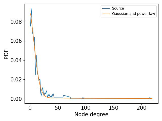
(3) Contact-tracing networks. We received anonymized high-level statistical information about real contact tracing networks that included the distribution of node degree, transmission probability and mean number of interactions per day, collected during April 2020.
 |
 |
| (a) | (b) |
Fig. S2(b) presents the degree distribution in this data, and the transmission probability is presented in Fig. S2(a). The latter was derived based on the contact properties, such as the length and the proximity of the interaction. On average, interactions with a significant transmission probability were recorded per-person per-day. We generated random networks based on these distributions using a configuration model framework (Newman, 2010). The fitted model for the degree distribution is a mixture of a Gaussian and a power-law distribution
| (4) |
The fitted model for the transmission probability is a mixture of a Gaussian and a Beta distribution
| (5) |
Evaluation on CT data. Due to privacy constraints, we did not have access to “live” CT graphs. We used these statistics to generate topologically similar synthetic graphs. Likewise, we simulated activity patterns based on activity statistics of the real CT network.
D.2 Epidemic test prioritization baselines
A. Preprogrammed Heuristics. The most prevalent baseline, used in practice nowadays in a few countries and circumstances, is based on the proximity of a node to infectious node. We compare with two such methods to ran k nodes. (1) Infected neighbors. Rank nodes based on the number of known infected nodes in their 2-hop neighborhood (neighbors and their neighbors). Each node is assigned a tuple , and tuples are sorted in a decreasing lexicographical order. A similar algorithm was used in (Meirom et al., 2015, 2018) to detect infected nodes in a noisy environment, and its error was shown to vanish asymptotically in the network size. (2) Probabilistic risk. Each node keeps an estimate of the probability it is infected at time . To estimate infection probability at time , beliefs are propagated from neighbors, and dynamic programming is used to analytically solve the probability update. See Appendix E for details. (3) Degree centrality. In this baseline high degree nodes are prioritized. This is an intuitive heuristic and it is used frequently (Salathé & Jones, 2010). It was found empirically to provide good results (Sambaturu et al., 2020). (4) Eigenvalue centrality. Another common approach it to select nodes using spectral graph properties, such as the eigenvalue centrality (e.g., (Preciado et al., 2014; Yang et al., 2020)).
The main drawback of these heuristic algorithms is that they do not exploit all available information about dynamics. Specifically, they do not use negative test results, which contain information about the true distribution of the epidemic over network nodes.
B. Supervised learning. Algorithms that learn the risk per node using features of the temporal graph, its connectivity and infection state. Then, nodes with the highest risk are selected. (5) Supervised (vanilla). We treat each time step and each node as a sample, and train a 3-layer deep network using a cross entropy loss against the ground truth state of that node at time . The input of the DNN has two components: A static component described in Section 4.1, and a dynamic part that contains the number of infected neighbors and their neighbors (like #1 above). Note that the static features include the, amongst other features, the degree and eigenvector centralities. Therefore, if learning is successful, this baseline may derive an improved use of centralities based on local epidemic information. (6) Supervised (+GNN). Like #5, but the input to the model is the set of all historic interactions of ’s and its -order neighbours and their time stamps as an edge feature. The architecture is a GNN that operates on node and edge features. We used the same ranking module as our GNN framework, but the output probability is regarded as the probability that a node is infected. (7) Supervised (+weighted degree). Same as #6, but the loss is modified and nodes are weighted by their degree. Indeed, we wish to favour models that are more accurate on high-degree nodes, because they may infect a greater number of nodes. (8) Supervised (+weighted degree +GNN). Like #6 above, using degree-weighted loss like #7.
The supervised algorithm is trained to optimize the model by minimizing the cross entropy loss function at every time step between the predicted probability that node will be infected to its groundtruth state :
| (6) |
In the unweighted cross entropy loss, all nodes are weighted equally, . We can strengthen this baseline by noting that we would like the model to be more accurate on high degree nodes, as they may infect a greater number of nodes. Hence, we weigh the contribution of a node to the loss term by its degree, . We refer to the latter algorithm as a degree weighted SL.
The main drawback of the supervised algorithms is that they optimize a myopic loss function. Therefore, they are unable to optimize the long term objective and consider the strategic importance of nodes.
Metrics. The end goal of quarantining and epidemiological testing is to minimize the spread of the epidemic. As it is unreasonable to eradicate the epidemic using social distancing alone, the hope is to “flatten the curve”, namely, to slow down the epidemic progress. Equivalently, for a simulation with fixed length, the goal is to reduce the number of infected nodes. In addition to the %healthy metric, defined in Sec. 5, we consider an additional metric, %contained: The probability of containing the epidemic. This was computed as the fraction of simulations having cumulative infected nodes smaller than a fraction . We focus on this metric because it captures the important notion of the capacity of a health system. In the 2-community setup, where each community has half of the nodes, a natural choice of is slightly greater than , capturing those cases where the algorithm contains the epidemic within the infected community. In all the experiments we set . The only exception is the three-communities experiments, in which we set the bar slightly higher than , and fixed .
D.3 Epidemic Test Prioriritzation - Additional Experiments
Epidemic slowdown. We investigated the progression of the epidemic under either RLGN or supervised+GNN algorithms. Figure S4 shows that the epidemic spread speed is slower under the RLGN policy in all graphs. In general, there are two extreme configuration regimes. First, the “too-hard” case, when the number of tests is insufficient to block the epidemic, and second, the “too-easy” case when there is a surplus of tests such that every reasonable algorithm can contain it. The more interesting case is the intermediate regime, where some algorithms succeed to delay the epidemic progression, or block it completely, better than other algorithms. Fig. S4(a) illustrates the case where the number of tests is insufficient for containing the epidemic, for all algorithms we tested. In Fig. S4(b), the number of tests is insufficient for SL to block the epidemic. However, with same number of tests, RLGN algorithm successfully contains the epidemic. Fig. S4(c) presents an interesting case where RLGN slows down the epidemic progression and reduces the number of total number of infected node, compared with SL, but RL does not contain it completely.
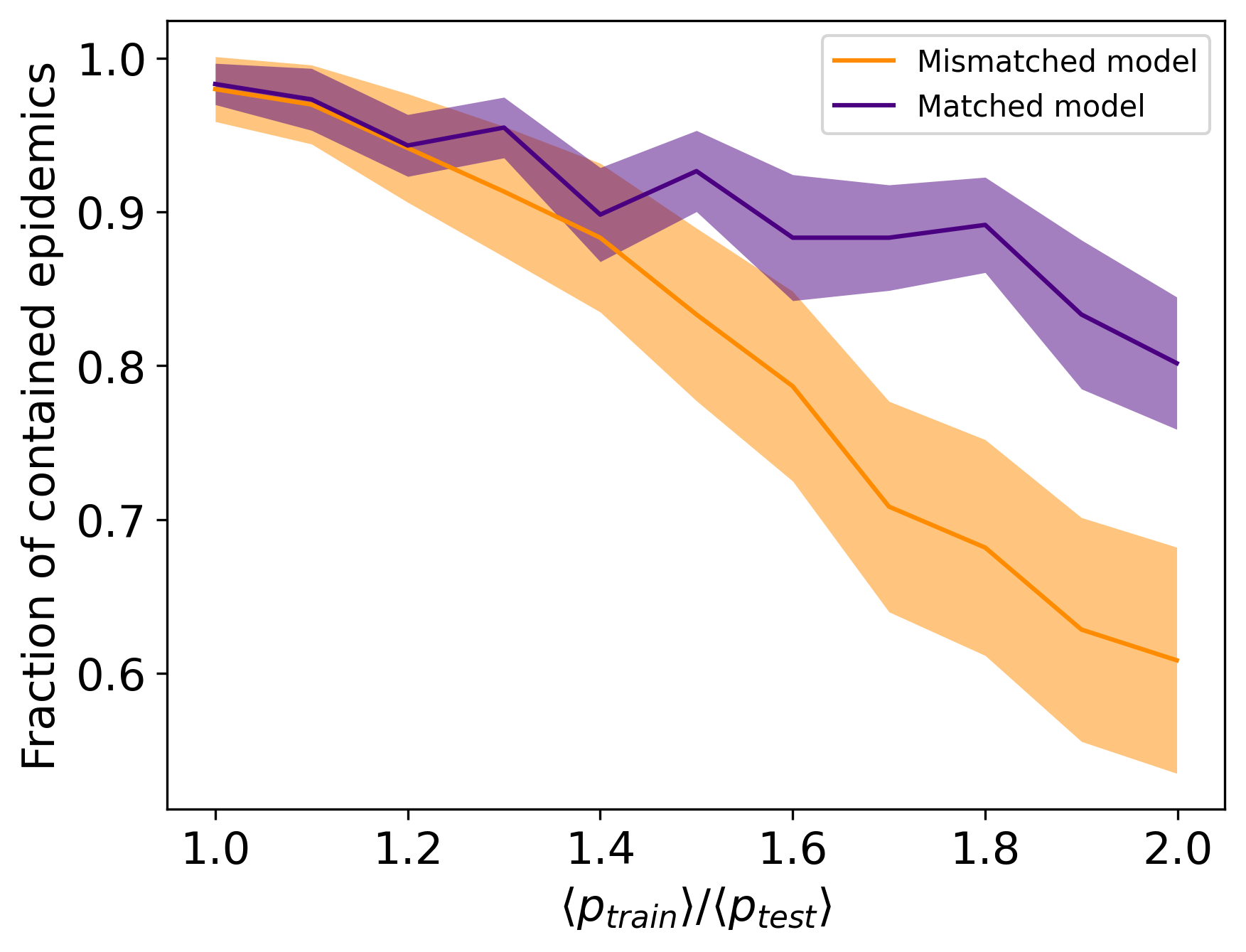
Epidemiological model variations. Figure S1(b) depicts a robustness analysis of RLGN for variations in the epidemiological model. One of the most difficult quantities to assess is the probability for infection per social interaction. Figure S1(b) shows that the trained model can sustain up to deviation at test time in this key parameter.
Graph size variations. We have tested the robustness of our results to the underlying graph size. Specifically, we compare the two best algorithms RLGN (#8) and SL+GNN (#4), using graphs with various sizes, from 300 nodes to 1000 nodes. Table S6 compares RLGN with the SL+GNN algorithm on preferential attachment (PA) networks (mean degree ). We provide results for various sizes of initial infection and number of available tests at each step. The experiments show that there is a considerable gap between the performance of the RL and the second-best baseline. Furthermore, RLGN achieves better performance than the SL+GNN algorithm with 40%-100% more tests. Namely, it increases the effective number of tests by a factor of .
Initial infection size. We also tested the sensitivity of the results to the relative size of the initial infection. Table S6 shows results when 4% of the the network was initially infected, as well as for 7.5% and 10%. The results show that RLGN outperforms the baselines in this wide range of infection sizes.
D.4 Influence Maximization - Additional Experiments
We presented two natural extensions to the Independent Cascades model. In Table 3 in the main paper we presented the results of the IC(geometric) model. Table S1 presents the results of the IC(constant) model. In both cases, RLGN often outperform the state-of-the-art algorithms. In both simulations, the neighbor influence probability was , the agent’s success probability for setting a node to Influenced state was , and the probability that an influenced node will reveal its state was .
We follow with a comparison of the performance of the various algorithms on the Linear Threshold model (Table S2). Here, RLGN clearly outperformed the other baselines. The main reason to the increased gap is that a Linear Threshold model contains more parameters, as each edge and is associated with a random weight and each node is assigned a peer resistance value. RLGN, as a trainable model, is able to uncover relevant patterns, while the other algorithms fail to do so. Table S2 also shows that the RLGN performs better thatn the baselines over a variety of the dynamic model parameters.
| gemsec-RO | ca-HepTh | ca-GrQc | ||
|---|---|---|---|---|
| LIR | ||||
| LIR (filtered) | ||||
| Degree | ||||
| Degree Discounted | ||||
| Eigenvector | ||||
| RLGN |
| ca-GrQc | gemsec-RO | ca-HepTh | ||
|---|---|---|---|---|
| LIR | ||||
| LIR(filtered) | ||||
| Degree | ||||
| Degree Discounted | ||||
| Eigenvector | ||||
| RLGN |
| ca-GrQc | gemsec-RO | ca-HepTh | ||
|---|---|---|---|---|
| LIR | ||||
| LIR(filtered) | ||||
| Degree | ||||
| Degree Discounted | ||||
| Eigenvector | ||||
| RL+GNN |
D.5 Ablation Studies
Mapping scores to action distribution.
We compare the performance of our score-to-probability function (calibrated-scores) to the popular softmax (Boltzmann) distribution. In practice, in most instances, we were unable to train a model using the softmax distribution as the neural network weights diverge. Fig. S5 presents the training curve in one of the few instances that did converge. It is clear that the model was not able to learn a useful policy while using the calibrated-scores probability function resulted in a corresponding value of more than . We also compare our approach with the recent escort transform (Mei et al., 2020), a state-of-the-art score-to-probability method. As shown in Fig. S5, our method outperforms the escort transform in this problem.
| # training epochs | ||
|---|---|---|
| Sigmoid | 1210 | |
| GRU | 810 | |
| norm. | 500 |
Normalization in scale-free networks.
We compared the suggested normalization to a number of other alternative normalization methods. (1) Applying a sigmoid layer after the hidden state update module . (2) Replace the hidden state update module with a GRU layer. (3) Apply normalization to each feature vector (similarly to (Hamilton et al., 2017)) (4) Normalize the feature vector matrix by its norm. These four normalization schemes span three different types of normalization: single-feature normalization (1+2), vector normalization (3), and matrix normalization (4).
Table S3 presents the score after training and the number of training steps required to complete training. Method (4) was unstable and training did not converge, therefore it was omitted from the table. The main reason for the training time difference is that without normalization, the DNN weights’ magnitude increases. In a GRU module, or with a direct application of a sigmoid layer, the features pass through a sigmoid activation function. When the magnitude of the input to this layer is large, the gradient is very small due to the sigmoid plateau. This substantially slows down the learning process.
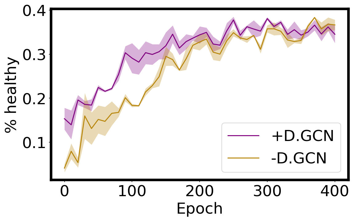
| #Nodes | #Edges | |
|---|---|---|
| CA-GrQc | 5242 | 14496 |
| Montreal | 103425 | 630893 |
| Portland | 10000 | 199167 |
| 32430 | 54397 | |
| GEMSEC-RO | 41773 | 222887 |
| %contained | 2 communities | 3 communities |
|---|---|---|
| Tree-based model | ||
| Counter model | ||
| Degree centrality | ||
| Eigenvector centrality | ||
| Supervised (vanilla) | ||
| Supervised +GNN | ||
| Supervised +degree | ||
| Supervised +GNN+deg | ||
| RLGN (Vanilla) | ||
| RLGN full (ours) | 881 | 5313 |
| Init. infection size 5% | Init. infection size 7.5% | Init. infection size 10% | ||||
|---|---|---|---|---|---|---|
| %healthy | %contained | %healthy | %contained | %healthy | %contained | |
| SL, | ||||||
| SL, | ||||||
| SL, | ||||||
| RLGN, | ||||||
| Init. infection size 5% | Init. infection size 7.5% | Init. infection size 10% | ||||
|---|---|---|---|---|---|---|
| %healthy | %contained | %healthy | %contained | %healthy | %contained | |
| SL, | ||||||
| SL, | ||||||
| SL, | ||||||
| RLGN, | ||||||
| Init. infection size 5% | Init. Infection size 7.5% | Init. infection size 10% | ||||
|---|---|---|---|---|---|---|
| %healthy | %contained | %healthy | %contained | %healthy | %contained | |
| SL, | ||||||
| SL, | ||||||
| SL, | ||||||
| RLGN, | ||||||
| (a) GamesecRO | (b) Email | (c) ca-GrQc |
|---|---|---|
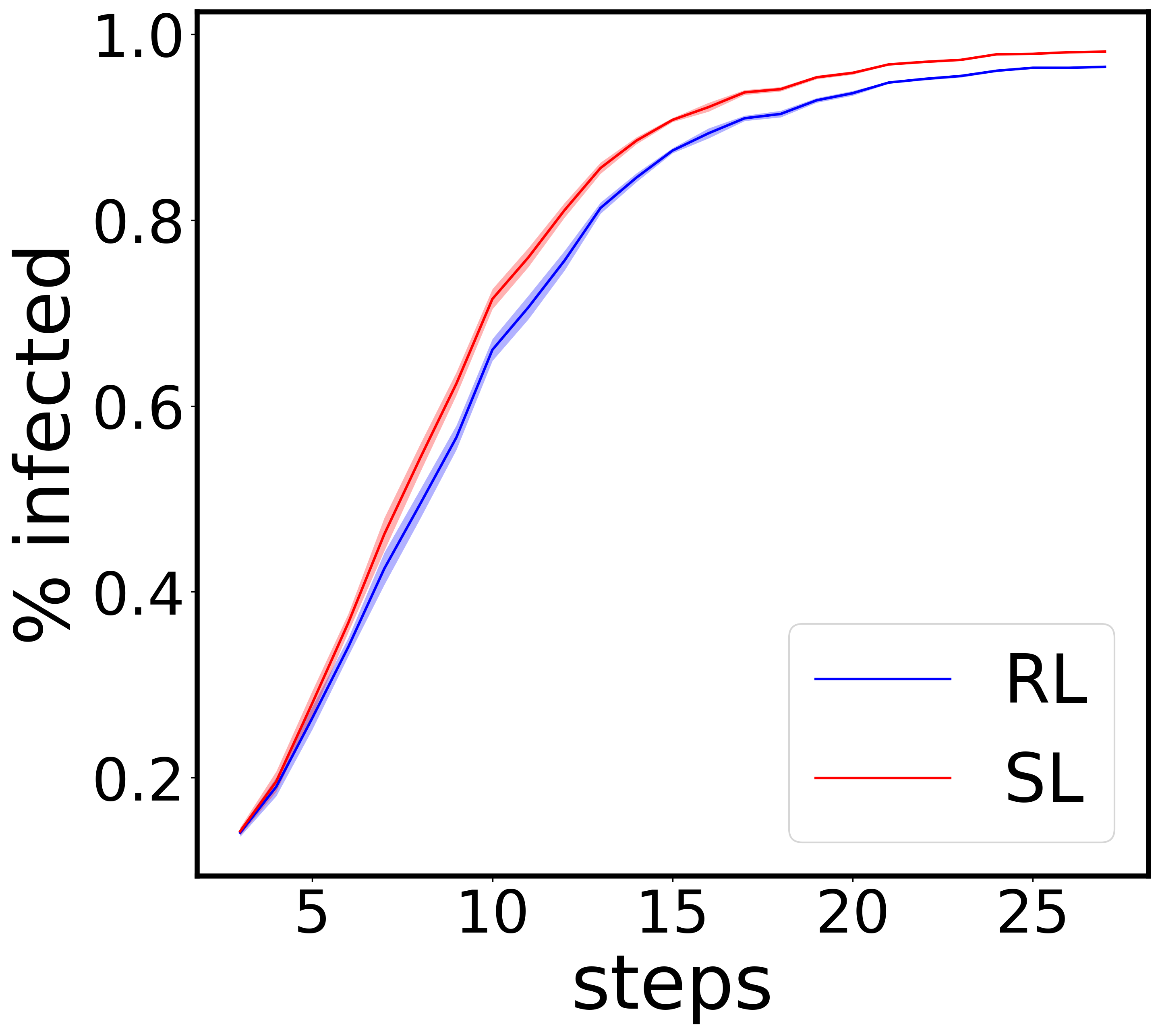 |
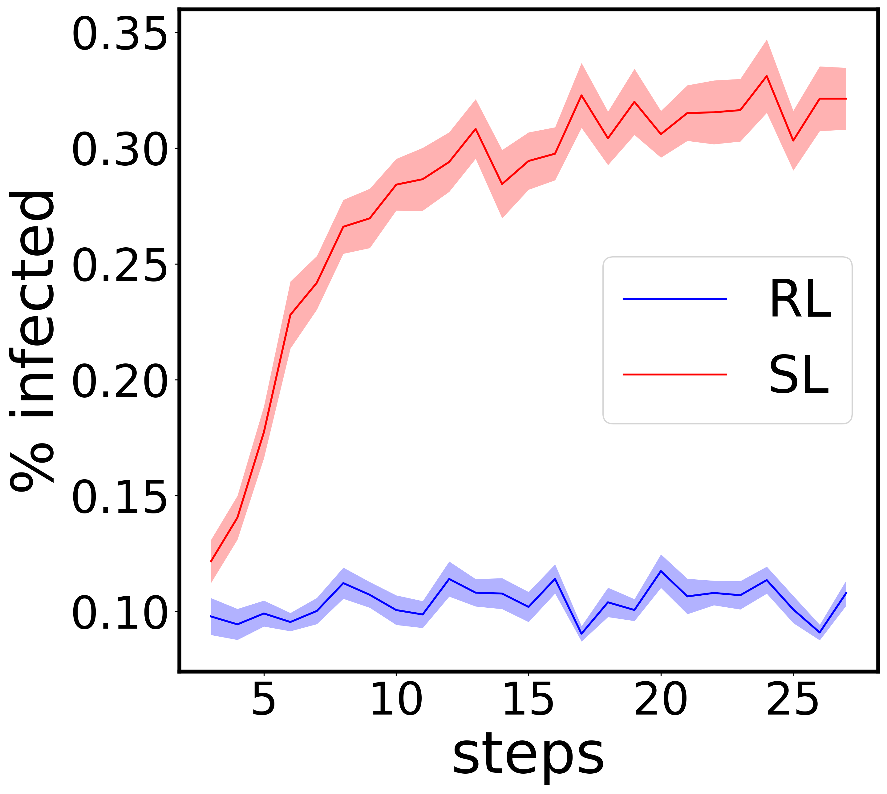 |
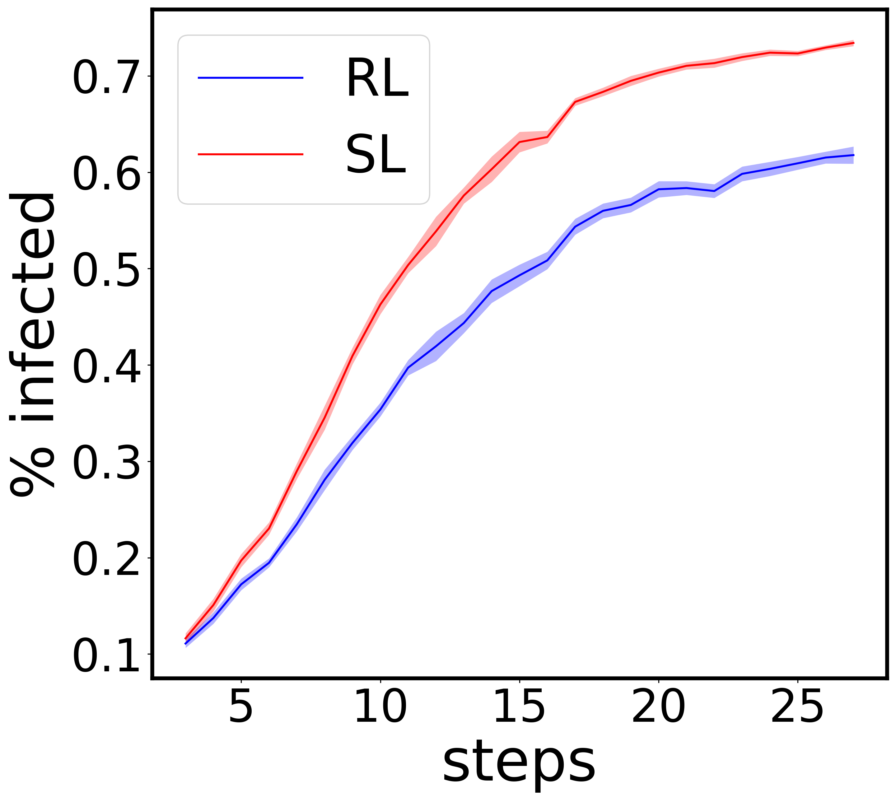 |
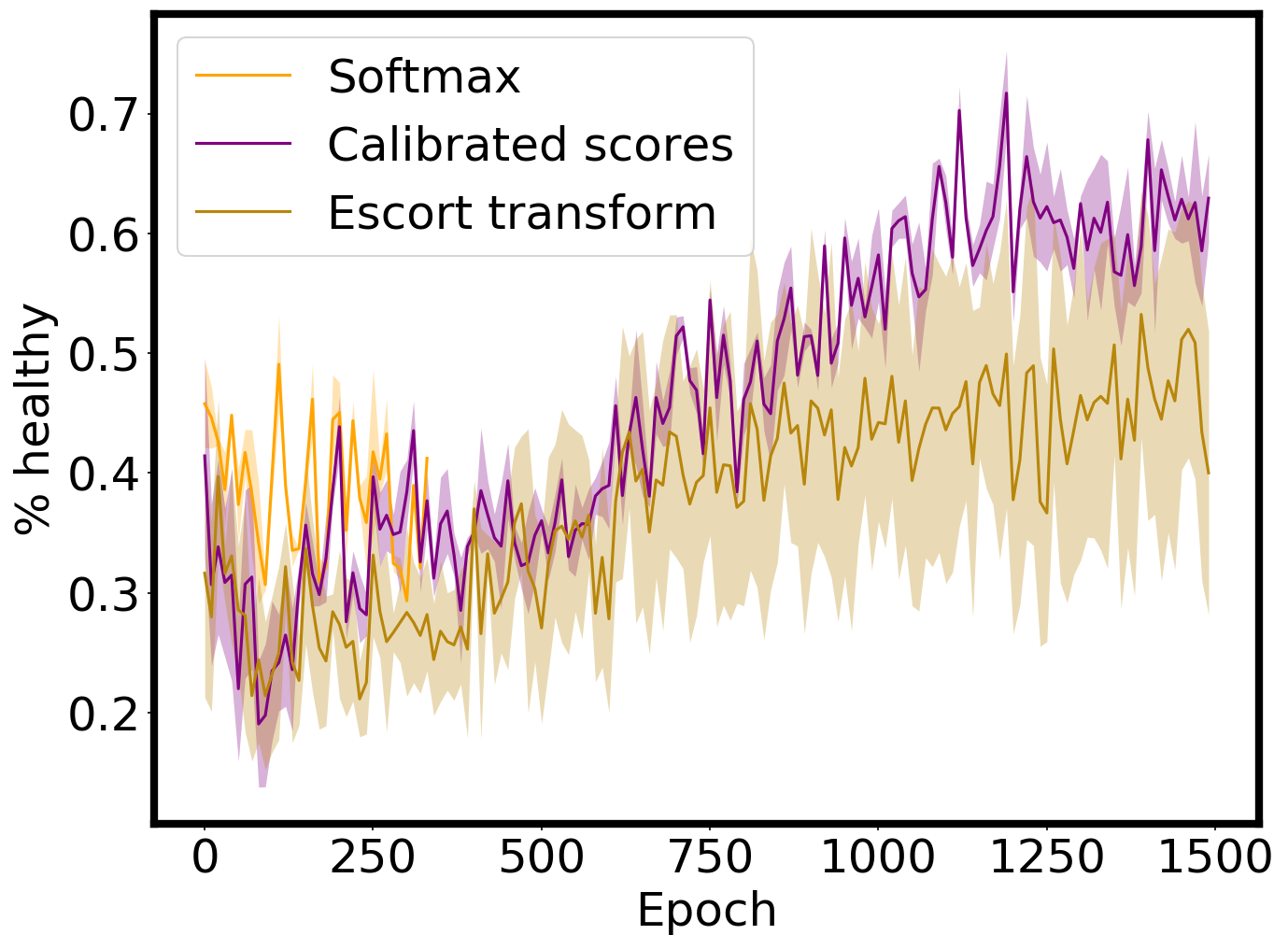
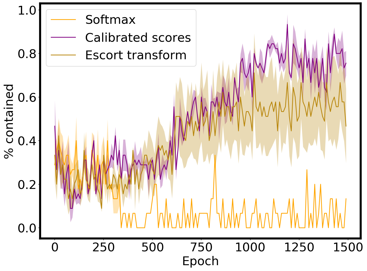
D.6 Network architecture
The architecture of the ranking module is shared by algorithms #4, #6 and #8 with slight variations indicated below.
Input.
We encode the dynamic node features as follows. Epidemic test priorization: A one hot hot vector of dimension . Each of the first three elements corresponds to one of the three mutually exclusive options, which depends on the previous step: untested, tested positive, tested negative. The last entry indicates whether a node was found positive in the past. Influence maximization: A one hot hot vector of dimension . Similarly, the first two elements indicate whether a node has indicates it is influenced in the previous step or not, and the last element whether it indicated so in the past. The static node features, , are common to both problems. As described in the main paper, topological graph centralities (betweenness, closeness, eigenvector, and degree centralities) and random node features. The graph centralities are standard metrics, and were calculated using NetworKit. An ablation study showed a maximal performance difference of 2% between different centralities subsets and was statistically insignificant.
Local Diffusion GNN.
This module is composed of a single graph convolutional layer. The input features are the last time step node features. The number of output features is 64.
Long Range Information GNN.
Each message passing module contains one hidden layer, where the number of hidden features is 64. After both the hidden and the last layer we apply a leaky ReLu layer with leakage constant . After aggregating the result using the addition aggregation function, we apply an additional MLP with one layer (linear+ReLu) on the resulting feature vector. The number of output features is 64. The value of , the information window size, was 7 in all our experiments.
We experimented with the numbers of stacked modules (layers). We found that performed slightly better than but training was considerably slower because the batch size had to be reduced. We therefore used in all experiments reported.
Hidden state update.
The hidden state MLP is composed of a single linear layer follows by a ReLu activation layer. To keep the resulting hidden feature vector (of dimension 64) norm under check, an additional normalization scheme is then applied. This module was replaced by a GRU layer in the ablation studies.
Output layer.
The last module is a single linear layer, with an output dimension as the number of the nodes in the graph.
Learning framework.
D.7 Training protocol
Initializaition. The initialization depends on the problem setup. Each influenced node signal with probability at each turn. In the epidemic tests prioritization setup we trained the RL and SL algorithms by generating random networks and initializing each network by selecting for each instance a random subset of infected nodes. We propagate the epidemic until it spans at least infected nodes (for at least steps), and randomly detect a subset of the infected nodes of size . The initialization for the Influence Maximization setup is simpler, and conclude in generating a random network.
At each step, in all algorithms but RL, we pick the top rated nodes. In RL, we perform the same procedure during the evaluation phase, while during training we sample nodes using the score-to-probability distribution.
Each model was trained for at most 1500 episodes, but usually, training was completed after 1000 episodes. Each episode contained 1024 steps, collected by 4 different workers. As our network contains a recurrent module, we propagate each sample in the buffer for three steps, in a similar fashion to R2D2.
For each setup we described, at least three models were trained using different seeds, and the results are the average over the performance of all models. The errors are the standard deviation of the mean. over at least 100 evaluation episodes for each model.
Each episode lasted for 25 steps, each corresponds conceptually to a day. The transition time from the latent to the infectious state was normally distributed with a mean of two steps and a standard deviation of 1 step, corresponding to real-world values. The advantage was calculated using the Generalized Advantage framework with parameters
Table S7 presents the simulation parameters used in the main paper. We shall make the repository and code available online.
| minimal #propagation steps () | 4 |
|---|---|
| minimal #infected component size () | communities: 4 (same community) |
| preferential attachment: 5% | |
| contact tracing: 7% | |
| Learning rate | |
| 0.97 | |
| 0.99 | |
| Entropy loss weight | 0.01 |
| Value loss weight | 0.5 |
| Probability distribution of | |
| Batch size | 256 (128 if #nodes) |
| 3-communites SBM matrix | |
| 2-communites SBM matrix |
Appendix E The tree model baseline
In this appendix We describe our tree model baseline (algorithm #1). Consider an epidemic propagating on a tree, and assume there is a single initially infected node (”patient zero”). In this case, there is a single path from the infection source to every node in the graph and we can we can analytically solve for the probability a node is infected, given that the root of the tree was infected at time . This model is useful when the underlying network is locally a tree, i.e, that for every new infected node there is w.h.p just one node which may have infected it.
We start with a simple case.
E.1 Simple case: No latent state
Let us first consider a simple model in which the epidemic spreads on a tree like structure with a single epidemic source, a.k.a. patient-zero, as the root. For now, let us assume there is no latent state.
Our goal is to calculate the probability that a node will be infected at time
For every node there is a single path from the node to the root, denoted by . Let us assume the path is . Assume that in a sequence of interactions between node and occurred at discrete times , and that each interaction is characterized by an infection probability . We evaluate by induction. For abbreviation, we write and denote the event as .
Our key result is that The state of node at the time of interaction is a function of its state at penultimate interaction time , the interaction transmission probability , and the predecessor node state at time , .
The first term is the probability to get infected at the interaction, and the second term is the probability to get infected before hand. We shall now prove this result.
Proof.
We can write the conditional probability using a graphical model decomposition and obtain
| (7) | ||||
since if the ancestor node is not in an infectious state, the decedent can not be infected. Denote the indicator that interaction was able to transmit the epidemic as . We have,
As, for an infection event to take place at it must be that node was infected at , node was healthy beforehand, and that the interaction resulted in an infection. We can now write this as
| (8) | ||||
The transition from the first line to the second is due to the independence of the interaction infection probability with the history of the participating parties. The third line is Bayes’ theorem. If a node is infected at time , it will be infected later on at , as expressed in line 4. The last line is the complete probability formula.
We rewrite as
The transition from the first line to the second line is a complete probability transition. The third line is due to the fact that if was not infected at time , clearly could not be infected before . We have
Therefore, given for all and for all , we can directly calculate the infection probabilities, given the initial condition: .
We can write the partial density function of as , and obtain: . This allows us to write this with an intuitive formulation
The first term is the probability to get infected at the interaction, and the second term is the probability to get infected before hand.
∎
E.2 Full analysis with latent states
We now discuss the case where a node can be in a latent state. The main difference is that the complement of the infectious state is composed of two states, healthy , and latent . We shall denote all the non-infecting states as and all the infected states as , and sometime abuse the notation by writing . We denote the transmission delay from the latent to infectious state as .
As before, we are interested in the probability that
The derivation below shows that, similar to the previous case, we can solve for this probability using dynamic programming. The end result is that
with
and
Therefore, as before, given and for all , we can propagate and calculate and .
Proof.
We start with an equation equivalent to Eq. 7,
where we kept the definition of . Therefore, almost identically,
Eq. 8 follows up to the last line, where:
and,
To summarize, we obtain:
Let us denote the probability density function that an infection occurred during interaction as
| (9) |
We have,
The transition from the latent state to the infected state follows:
| (10) |
while
| (11) |
Therefore, given and for all , we can propagate and calculate and . ∎