Interpretable Neural Networks for Panel Data Analysis in Economics

Abstract

The lack of interpretability and transparency are preventing economists from using advanced tools like neural networks in their empirical research. In this paper, we propose a class of interpretable neural network models that can achieve both high prediction accuracy and interpretability. The model can be written as a simple function of a regularized number of interpretable features, which are outcomes of interpretable functions encoded in the neural network. Researchers can design different forms of interpretable functions based on the nature of their tasks. In particular, we encode a class of interpretable functions named persistent change filters in the neural network to study time series cross-sectional data. We apply the model to predicting individual’s monthly employment status using high-dimensional administrative data. We achieve an accuracy of 94.5% in the test set, which is comparable to the best performed conventional machine learning methods. Furthermore, the interpretability of the model allows us to understand the mechanism that underlies the prediction: an individual’s employment status is closely related to whether she pays different types of insurances. Our work is a useful step towards overcoming the “black box” problem of neural networks, and provide a new tool for economists to study administrative and proprietary big data.

November 2020

1 Introduction

Traditionally, economists have relied on interpretable models like linear or logistic regressions, which provide clear insights on the causal or statistical relationships in small datasets [2, 22]. Recently, the use of administrative and proprietary big data has led to lots of exciting work in empirical economics [9, 7, 15, 19]. Though such datasets enjoy the richness of variables and large sample size, advanced tools like neural networks have not been adopted widely in their analysis as expected. Methodologically, there have been some attempts to bring machine learning tools to economic analysis. However, most of those successful applications are limited to relatively simple models like Lasso, ridge regressions or decision trees [16, 6, 13]. Economists are still nervous about using more advanced tools like neural networks, since they mostly deliver outcomes from a complicated black box without transparency or interpretability [3], even though they enjoy better capability to fit data well than traditional econometric models.

To address this dilemma, we propose a new class of interpretable neural network models. Our model allows us to take advantage of the high accuracy of neural networks, while remaining interpretable like linear or logistic regressions. To this end, we design a modified version of neural networks: all layers except the last one encode various interpretable functional forms with unknown parameters, while the final layer is a logistic function that only takes a regularized number of neurons as inputs. As is shown in Figure 1, our model can essentially be written as a simple logistic function of a limited number of interpretable features (red circles), which makes it more interpretable than conventional neural networks. Under this general formulation, researchers can design different interpretable functional forms based on their own tasks. In this paper, we design a class of persistent change filters as part of the network, which turns out particularly helpful in time series cross-sectional data analysis.

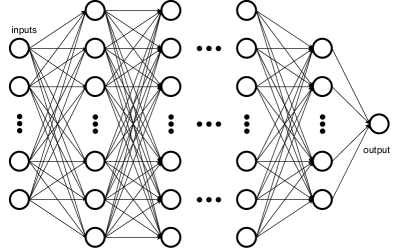
(a) Conventional Neural Networks

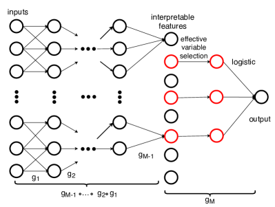
(b) Interpretable Neural Networks

Figure 1: Comparison of Conventional Neural Networks (left) and Interpretable Neural Networks (right).

The interpretable neural network model we propose satisfies all the three desiderata for interpretable machine learning models [17]. First, it has high “predictive accuracy” due to the capability of its multi-layer architecture to fit data well. Second, it has high “descriptive accuracy” since the model structure is designed to be interpretable. Third, it meets the “relevancy” requirement. Reseachers can design different interpretable functional forms in different tasks, so that the model estimates can deliver relevant knowledge. Beyond these three desiderata, our model estimates are robust to data missing problems, which is crucial if we expect to get reliable interpretations of the model.

As an application, we use the interpretable neural network models with persistent change filters to predict individual’s monthly employment status using high-dimensional administrative data in China. We achieve an accuracy of 94.5% on the test set, which is comparable to the best-performing conventional machine learning methods. In addition, we clearly understand how the model predicts an individual’s employment status with her payment records of different types of insurances. Both the accuracy and the interpretability are robust subject to data missing problems.

This paper contributes to the literature with the following distinct features. First, we expand the machine learning toolbox for economists [16, 6, 13, 21] by introducing a modified neural network model that achieves high accuracy without sacrificing interpretability and transparency. Second, we contribute to the large literature on interpretable machine learning. Previous work in computer vision and natural language processing [8, 25, 14] mostly focus on interpreting how hidden units of neural networks represent local features of images and texts. In this paper, we propose an interpretable model to study panel data, to help people understand the mechanisms behind the collective human behavior. In the terminology of the overview paper on interpretable machine learning [17], our model delivers “model-based interpretability”, which is different from work that delivers “post hoc interpretability” by approximating outcomes from complicated models with simple functions. Last but not least, the application of our model to predicting individual employment status with China’s administrative data also contributes to the large literature on China’s unemployment study in the absence of reliable official statistics [11, 10]. Our work stands out in this literature as a novel application of machine learning methods on administrative big data, rather than traditional national account approach on household survey data.

The remaining of the paper is organized as follows. In Section 2, we present the architecture of the interpretable neural network model. In particular, we encode a class of interpretable functions named persistent change filters in the model to study panel data. In Section 3 we exhibit the virtues of the model by applying it to predict individual’s employment status in a large administrative dataset. Finally we conclude with discussions on the future work.

2 Interpretable Neural Networks for Panel Data

2.1 Interpretable Neural Networks: General Formulation

We first lay down the general formulation for the interpretable neural network model. For observation $i$, we write the model as $y_{i}=g(\bm{x}_{i},\theta)$, where $g$ shares the multi-layer structure as conventional neural networks $g=g^{(M)}\circ g^{(M-1)}\circ\dots\circ g^{(1)}$.

For the first $M-1$ layers, $g^{(M-1)}\circ\dots\circ g^{(1)}$ are multi-dimensional differentiable interpretable functions with unknown parameters. Here the functional forms should be designed based on the nature of tasks, since interpretable functions in computer vision may look very different from those in economics. These functions map the original variables into high-dimensional interpretable features. The last layer $g^{(M)}$ is a logistic function with these interpretable features as inputs. To make the final model more interpretable, we require the final layer to only take a small number of interpretable features as inputs. This is achieved by adding a Lasso [20] or group Lasso [24] type of penalty on the parameters of the final layer to the loss function:

$$L(\theta,\phi)=\operatorname{\mathbb{E}}_{X,Y}\text{Loss}(g(x,\theta),y)+\lambda\mbox{penalty}(g^{(M)})$$ (1)

Here $\lambda$ is a hyperparameter. The full architecture of interpretable neural network $g$ is in the right panel of Figure 1. Since all components are differentiable in loss function (1), the model can be trained like a conventional neural network with gradient descent algorithms like Adam [12].

2.2 Interpretable Neural Networks for Panel Data

Now we design an interpretable functional form for panel data analysis. Consider a model $y_{it}=g(\mathbf{x}_{it},\theta)=g^{(M)}\circ g^{(M-1)}\dots\circ g^{(1)}$, where $y_{it}$ is the outcome for unit $i$ at time $t$ and $\mathbf{x}_{it}$ are high dimensional inputs. We choose $M=4$ and design functional forms for $\{g^{(m)}\},m=1,2,3$ as below.

1. $g^{(1)}$: Decision-tree-like splitting $\text{Sp}(x)=\mbox{Sigmoid}(cx+d)$. For $x\in\mathbb{R}^{1}$, a sigmoid function can function as a decision-tree-like splitting operator like a differentiable indicator function [23]. For example, if $c$ is close to 1 and $d$ is a large negative number, the output can be close to 0 and 1 to discriminate whether $x$ is smaller or larger than a threshold. Here $c$ and $d$ are unknown parameters.

2. $g^{(2)}$: Dimension reduction $\text{Re}(\mathbf{x})$. For $\mathbf{x}\in\mathbb{R}^{m}$, define $\text{Re}(\mathbf{x}):\mathbb{R}^{m}\rightarrow\mathbb{R}^{n}(n\ll m)$ as a certain dimension reduction function with unknown parameters. For example, $\text{Re}(\mathbf{x})$ could be linear combination with sparse inputs, and the linear coefficients are unknown parameters.

3. $g^{(3)}$: persistent change filter $\mathcal{D}(\mathbf{x})$. Now we introduce a class of interpretable functions named persistent change filter, which turns out helpful in panel data analysis. $\mathcal{D}(\mathbf{x})$ also include unknown parameters.

2.3 A Class of Interpretable Functions for Time Series Data: Persistent Change Filter

For a particular time series for some individual unit $i$ (the $i$ subscript is omitted here for simplicity), $x_{\tau}\in[0,1],\tau=1,2...t$, we define the persistent change filter $z_{t}=\mathcal{D}(\{x_{\tau}\}_{\tau=1}^{t})=p_{t}-q_{t}$, where:

$$p_{1}=x_{1},p_{\tau+1}=[1+k(x_{\tau+1}-1)]p_{\tau}+x_{\tau+1}$$

$$q_{1}=1-x_{1},q_{\tau+1}=[1+k(-x_{\tau+1})]q_{\tau}+(1-x_{\tau+1})$$

Here $k\in[0,1]$ is an unknown parameter. Then we can map the original time series $\{x_{t}\},t=1,2,...,T$ to a persistent change filter time series $\mathcal{D}(\{x_{\tau}\}_{\tau=1}^{t}),t=1,2,...,T$. The definition of the persistent change filter $\mathcal{D}$ is motivated by identifying a persistent change in time series data. We illustrate this idea first with two examples and formalize with a proposition.

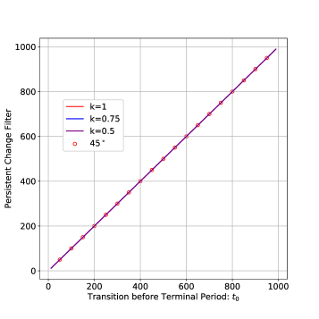
(a) Persistent Change Filter on Data without Missing Problem

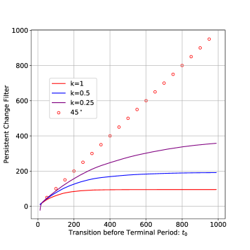
(b) Persistent Change Filter on Data with Missing Problems

Figure 2: Persistent Change Filter Captures the Duration of a Persistent Change

Example I For a binary time series $x_{t}\in\{0,1\},t=1,2...T=1000$. $x_{t}$ begins with 0 for some periods, and persistently switch to 1 for the last $t_{0}$ periods: $x_{t}=\mathbbm{1}[t>T-t_{0}]$. We plot the persistent change filter on the entire time series $\mathcal{D}(\{x_{\tau}\}_{\tau=1}^{T})$ against the number of periods $t_{0}$ between the transition and the terminal period in the left panel of Figure 2. We find that no matter what smoothing variable $k$ we choose, the persistent change filter fits perfectly with $t_{0}$ on the 45^∘ line. This implies that the persistent change filter captures the duration of a persistent change in such a binary time series $0,...,0,1,1,...,1$.

Example II In real world, such perfect binary data may not exist. Consider time series $x_{t}$, where everything is the same as Example I, except that a random 5% of $x_{t}$ are replaced with $x_{t}=0.9$ when $t>T-t_{0}$ to mimic an abnormal data or data missing problem. Then we plot the persistent change filter $\mathcal{D}(\{x_{\tau}\}_{\tau=1}^{T})$ against $t_{0}$ for different choices of $k$ in the right panel of Figure 2. For the the persistent change filter without any smoothing (i.e. $k=1$), the plot deviates from the 45^∘ line significantly. When $k$ decreases, the plot gets closer to the 45^∘ line. So an optimal choice of $k$ would help capture the duration of a persistent change in such a time series with potential data issues. To note, $k$ would be left as an unknown parameter that our model would learn from the data.

We formalize the examples above with the following proposition:

Proposition 2.1.

When $k\rightarrow 1$, $p_{T}$ uniformly converges to $\mathcal{D}^{(0)}$ defined as below:

$$\mathcal{D}^{(0)}(x_{T},x_{T-1}...x_{1})=\sum_{i=1}^{T}\prod_{j=1}^{i}x_{T-j+1}.$$

What does $\mathcal{D}^{(0)}$ means for the time series? Consider the binary time series $x_{t}\in\{0,1\},t=1,2...T$, $\mathcal{D}^{(0)}$ is the lasting time periods for recent $x_{i}$’s to be 1. In other words,

$$\mathcal{D}^{(0)}(x)=m\ \Longleftrightarrow\ x_{T}=x_{T-1}...=x_{T-m+1}=1,x_{T-m}=0$$

Thus $\mathcal{D}^{(0)}$ gives information on the lasting time since the most recent period when the binary time series persistently switch to 1. For continuous $x_{t}$ in $[0,1]$, $\mathcal{D}^{(0)}$ is differentiable at any point, which means it could be part of a trainable model. However, $\mathcal{D}^{(0)}$ only captures the jumps from low values to high values, so we extend $\mathcal{D}^{(0)}$ to $\mathcal{D}$ so that it can capture both persistent jumps and drops in the time series. This is the $q_{t}$ term in the formulation. As is discussed above, we also add the trainable smoothing parameter $k$ to adjust for data missing or abnormal data problems. For a more elaborate discussion and the origins of the persistent change filter, please refer to Supplement D.

3 Application

3.1 Employment Status Prediction with Interpretable Neural Networks

In this section, we apply the interpretable neural network model for panel data to predict individual’s monthly employment status with administrative data. The data come from a four-million population city in China, and includes basic demographic information (age, family relations, gender, education, etc.), as well as individual level monthly payments to six different kinds of social insurances and the Housing Provident Fund (HPF). With all these features, together with employment/unemployment labels on part of the sample (about 400,000 individuals are labelled every month), we construct an interpretable neural network model to predict employment status of all the individuals in the population each month. With the prediction results, we can calculate unemployment rate on the whole population as an important economic indicator for policy makers. This application is novel and important given the unreliability of China’s official unemployment statistics [10].

For individual $i$ in calendar month $t$, her employment status is denoted as $y_{it}\in\{0,1\}$, where 1 and 0 correspond to being employed and unemployed respectively. Her payment amounts for different insurances, among other individual features are denoted as $x_{ijt}$ where $j=1,2...m$ correspond to different features. To predict $y_{it}$, we stack features of the individual in the past $s$ period as model inputs, denote as $\tilde{\mathbf{x}}_{it}=(x_{ij\tau})$ where $j=1,2...m,\tau=t,t-1,...,t-s+1$.

Following Section 2.2, we write the model as $P(y_{it}=1|\tilde{\mathbf{x}}_{it})=g(\tilde{\mathbf{x}}_{it},\theta)$ where $g=g^{(4)}\circ g^{(3)}\circ g^{(2)}\circ g^{(1)}$. The original input variables of $g$ is a $ms\times 1$ vector:

$$\tilde{\mathbf{x}}_{it}=\left(x_{ij\tau}\right)\text{ where }j=1,2\ldots m,\tau=t,t-1,\ldots,t-s+1.$$

Here we use monthly payment data of various social insurances and the HPF from July 2016 to December 2017 to construct $\tilde{\mathbf{x}}_{it}$, so $m=7$ is the number of insurances to pay and $s=6$ denotes the lagged periods we consider in model inputs. With the administrative data in Section 3.1, . To construct a balanced data sample, we randomly select 20,000 employed observations and 20,000 unemployed observations. Both positive and negative samples are evenly divided into two parts to get the training set and the test set.

3.2 Model Results

To evaluate our model, we will compare it with other interpretable models (logistic regressions) as well as more complicated models (random forests or neural networks). These models require handcrafted features as model inputs. Based on the descriptive statistics and domain knowledge (see the details in Supplement A) on this problem, we construct the following features:

1. “Insurance count” (IC). The number of types of insurances the individual pays in period $t$.

2. “Naive persistent change” (NPC). For each kind of insurance, we construct the “naive persistent change” $\mathcal{D}^{(0)}(x_{t},x_{t-1},...,x_{t-s+1})$ following the definition in Proposition 2.1, where $x_{\tau}$ is a binary variable on whether the individual does not pay for a specific insurance in period $\tau$. Different from the persistent change filter, these “naive” measures do not incorporate any trainable parameters, and come directly from feature engineering.

3. “Payment change” (PC). We construct another “naive persistent change” variable taking the same expression based on the following binary time series $x_{\tau}$: whether the number of types of insurances the individual has paid is larger than 2. The feature with threshold 2 is constructed with insights from the descriptive statistics (see Supplement A).

With these features in hand, we compare the performance of the following 11 models:

1. The interpretable neural network (IntNN) model (1) we propose in this paper. No handcrafted feature is needed in this model.

2. Conventional interpretable model: logistic regression (Logistic) with (2) 7 “naive persistent changes”, “payment change” and insurance count; (3) 7 “naive persistent changes”; (4) “payment change” and insurance count; (5) “payment change”; (6) insurance count.

3. Conventional uninterpretable model: random forests (RF) and neural networks (NN) with (7) 7 “naive persistent changes”, “payment change” and insurance count; (8) 7 “naive persistent changes”; (9) “payment change” and insurance count; (10) “payment change”; (11) insurance count.

The predictive accuracy of the best-performing models under each category is reported in Table 1.

Table 1: Model Comparisons

Index	Model	Inputs	Test Accuracy
1	IntNN	-	0.94525
2	Logistic	NPC, IC, PC	0.9284
3		NPC	0.87035
4		PC, IC	0.81905
5		PC	0.81205
6		IC	0.84435
7	RF & NN	NPC, IC, PC	0.929
8		NPC	0.929
9		PC, IC	0.90605
10		PC	0.84435
11		IC	0.86395

Comparing the interpretable neural network model with logistic regression models, we find our model enjoys higher accuracy no matter how we feature engineer the logistic inputs. After hyperparameter tuning, random forest or conventional neural network models are more accurate than logistic regressions, but are still less accurate than our model, which might be a bit surprising to some readers. This comparison is actually in line with the finding of [18] which argues that the increase in interpretability may allow models to achieve higher accuracy in the test set than unrestricted models.

3.3 Model Interpretation

The interpretable neural network models deliver a clear mechanism behind the model outcome. Now we look into the model estimation results for each component of $g=g^{(4)}\circ g^{(3)}\circ g^{(2)}\circ g^{(1)}$, and interpret the model we obtain.

1. Decision-tree-like splitting $g^{(1)}$: For $\forall j,\tau$, ${x}_{ij\tau}^{(1)}=\mbox{Sigmoid}(c{x}_{ij\tau}+d)$.
   The estimates are $c=2.60,d=-41.46$. As is discussed in Section 2.2, with such $c$ and $d$, $g^{(1)}$ would transform small payment values to $0$, while keep large payment values close to 1. So, it approximates an indicator function of whether the individual pays each type of insurances.

2. Dimension reduction $g^{(2)}$: For $\forall\tau$, ${x}_{i\tau}^{(2)}=\mbox{Sigmoid}(w^{T}({x}_{ij\tau}^{(1)})_{j=1}^{m}+b)$.
   The estimates of the m-dimensional vectors $w=(-1.73,1.84,-4,0.64,0.62,-0.66,4.19)^{T}$, and each element corresponds to endowment insurance, urban working medical insurance, unemployment insurance, employment injury insurance, maternity insurance, urban non-working medical insurance, and the Housing Provident Fund (HPF) respectively. The intercept $b=3.67$.

   In this layer, we obtain a 1-dimension variable ${x}_{i\tau}^{(2)}$ from the linear combination of the 7-dimensional payment records after the decision-tree-like splitting. The output is positively correlated with payments of urban working medical insurance, employment injury insurance, maternity insurance, and the Housing Provident Fund (HPF), while negatively correlated with payments of endowment insurance, unemployment insurance, urban non-working medical insurance.

3. Persistent Change Filter $g^{(3)}$: $\tilde{{x}}_{it}^{(3)}=\mathcal{D}(({x}_{i\tau}^{(2)})_{\tau=t}^{t-s+1},k)$.
   The optimal smoothing parameter learnt from the original data is $k=0.999999$. As a persistent change filter on ${x}_{i\tau}^{(2)}$, a large positive $\tilde{{x}}_{it}^{(3)}$ corresponds to a persistent jump of ${x}_{i\tau}^{(2)}$, while a a large negative value corresponds to a persistent drop of ${x}_{i\tau}^{(2)}$.

4. Logistic regression $g^{(4)}$: $P(y_{it}=1)=\mbox{Sigmoid}(u\tilde{{x}}_{it}^{(3)}+v)$
   The estimates are $u=1.06,v=-2.18$. This is a differentiable version of linear transform with coefficient close to 1, which is similar to identity.

To summarize, our interpretable neural network model predicts individual’s employment status simply with the persistent change filter of a composite variable from a linear combination of whether an individual pay each type of insurance. The weights of the linear combination imply the relative importance of each insurance when predicting the employment status. From the model, we learn that when an individual that used to consistently pay urban working medical insurance, employment injury insurance, maternity insurance, or the Housing Provident Fund (HPF), but suddenly drop out from those insurance programs, there is a higher probability for her to become unemployed. Similarly, for individuals that are beginning to get enrolled in endowment insurance, unemployment insurance, urban non-working medical insurance, there is a higher probability for her to get unemployed. These model interpretations would be helpful for policymakers who hope to understand the accurate model predictions and design policies based on machine learning models.

3.4 Robustness of the Model

As is discussed in [17], an interpretable model should be robust to data missing or abnormal data problem. To mimic such scenarios, we randomly set 10% of all the payment records to 0, and train the same 11 models as in Section 3.2. The accuracy comparison results still hold. Also, the parameter estimates deliver qualitatively equivalent interpretations. The value of parameter $k$ in the persistent change filter becomes smaller to offset data missing. Please refer to Supplement C for more details.

4 Conclusion

In this paper, we propose a class of interpretable neural network models that can achieve both high prediction accuracy and interpretability. We first propose a general formulation of such neural networks, which begins with interpretable functional forms encoded in the first several layers, followed by the final layer with a regularized number of interpretable features as input. The model satisfies all the three desiderata for interpretable machine learning models [17]. Researchers can design different forms of interpretable functions based on the nature of their tasks. In this paper, we incorporate a class of interpretable functions named persistent change filters as part of the neural network to study panel data in economics.

As an application, we use the model to predict individual’s monthly employment status using high-dimensional administrative data in China. We achieve a high accuracy as 94.5% on the test set, which is comparable to the best-performing conventional machine learning methods. Furthermore, we interpret the model to understand the mechanisms behind. We find it accurately predicts individual’s employment status simply with the persistent change filter of a composite variable from a linear combination of whether an individual pay each type of insurance. The model deliver robust interpretations subject to potential data issues, and would be helpful for researchers and policymakers to understand useful information contained in the big administrative data.

This paper contributes to the machine learning toolbox of economists by introducing a modified version of neural networks that is both accurate and easy to interpret. The model can encode different interpretable functional forms that researchers may propose based on the nature of their own research tasks. For example, researchers who study default risks may propose specific functional forms that are interpretable on the loan data. With the massive use of administrative and proprietary big data in economics and policy research, lots of research could be done with this new tool.

Supplementary Materials

Appendix A Descriptive Statistics

Table 2 presents some descriptive statistics on insurance payment behaviors of both the employed and the unemployed sample.

Table 2: Descriptive Statistics

# of people that pay each insurance or HPF in the most recent period
	endowment	urban working medical	unemployment	injury
employed	10938	13737	19750	13503
unemployed	15026	0	19510	0
	maternity	non-working medical	HPF
employed	14167	0	9356
unemployed	0	42	443
# of types of insurances and HPF paid in the most recent period
	0	1	2	3
employed	0	5523	347	632
unemployed	369	4582	14708	341
	4	5	6	7
employed	140	7370	5988	0
unemployed	0	0	0	0

The upper panel is the number of employed and unemployed individuals that pay each type of the insurances in the most recent month in the sample. From this panel we can see that the unemployed individuals tend to pay endowment insurance, unemployment insurance and urban working medical insurance, while the employed individuals pay all the insurances except for urban non-working medical insurance, since they mostly prefer urban working medical insurance. The lower panel reports the number of types of insurances that paid by each employed and unemployed individual in the most recent month, we find that the employed individuals tend to pay more kinds of insurances. With the elbow method, we find 2 is a good threshold to discriminate the employed and the unemployed if we hope to do some traditional feature engineering, since most of the unemployed sample pay less or equal to 2 types of insurances.

Appendix B Interpretation Comparison: Our Model vs Logistic Regression

We compare our model with the logistic regression model with the “naive persistent changes” of seven kinds of insurances as model inputs. The definition of “naive persistent change” is in Section 3.2. The linear combination weights in $g^{(2)}$ of our interpretable neural network model and the logistic coefficients of each variable are in Table 3.

Table 3: Comparison: Interpretable Neural Networks vs. Conventional Interpretable Models

	Endowment	Working medical	Unemploy	Injury	Maternity	Non-work medical	HPF
IntNN	-1.73	1.84	-4	0.64	0.62	-0.66	4.19
Logistic	2.02	-0.61	0.32	-0.52	-1.16	1.53	-0.12

From Table 3, we find the interpretations of our model and the logistic regression model are qualitatively the same. As is discussed in the definition of “naive persistent change” in Section 3.2, larger naive persistent change means the individual switch from paying to not paying a specific type of insurance. Thus negative coefficients in the logistic regression imply a positive relationship between jumps in payments and the probability getting employed, which share the same interpretation as positive coefficients in our model. Here we find the signs of all the coefficients in the interpretable neural networks are exactly opposite to each other, which means they share exactly the same interpretation qualitatively.

Appendix C Robustness of the Model

C.1 Model Accuracy with Data Missing

The model we propose is robust to data missing or abnormal data problems. To check the robustness, we randomly set 10% of all the payment records to 0 as data missing. Then we rerun the same 11 models as in Section 3.2. The model accuracy results are in Table 4.

Table 4: Robust Model Comparisons: Our Model vs. Logistic Regression vs. Random Forest

Index	Model	Inputs	Test Accuracy
1	IntNN	-	0.92855
2	Logistic	NPC, IC, PC	0.91735
3		NPC	0.85805
4		PC, IC	0.79235
5		PC	0.7781
6		IC	0.84025
7	RF & NN	NPC, IC, PC	0.92715
8		NPC	0.917
9		PC, IC	0.85645
10		PC	0.84025
11		IC	0.84025

From Table 4, we can see that all the results are similar subject to the 10% data missing. Though data missing makes all the models worse off, our interpretable model remain the best performance among all the competitors. In the next section, we will see the model parameters are also robust, which delivers robust model interpretation for the problem.

C.2 Model Interpretation with Data Missing

In Section 3.3, we interpret our model clearly through the model structure. Besides transparency of the model structure, robustness is another important feature of model interpretability. In this section, we illustrate the robustness of our model with model parameters we estimate with 10% missing data in Section C.

1. Decision-tree-type splitting $g^{(1)}$: For $\forall j,\tau$, ${x}_{ij\tau}^{(1)}=\mbox{Sigmoid}(c{x}_{ij\tau}+d)$. The estimates are $c=2.76,d=-43.96$, which are both close to those in the baseline model.

2. Dimension reduction $g^{(2)}$: For $\forall\tau$, ${x}_{i\tau}^{(2)}=\mbox{Sigmoid}(w^{T}({x}_{ij\tau}^{(1)})_{j=1}^{m}+b)$. The estimates of the m-dimensional vectors $w=(-0.76,1.57,-2.12,0.55,0.5,-0.8,3.39)^{T}$. The intercept $b=2.87$. All the estimates are close to those in the baseline model.

3. Persistent Change Filter $g^{(3)}$: $\tilde{{x}}_{it}^{(3)}=\mathcal{D}(({x}_{i\tau}^{(2)})_{\tau=t}^{t-s+1},k)$. The estimated smoothing parameter is $k=0.89$, different from the baseline estimates 0.999999. This is totally sensible: due to data missing, we need to impose some smoothing to get a reasonable persistent change filter time series that predict the outcomes well. This also confirms the rationale of the persistent change filter definition, as is detailed discussed in Supplement D.

4. Logistic regression $g^{(4)}$: $P(y_{it})=\mbox{Sigmoid}(u\tilde{{x}}_{it}^{(3)}+v)$. The estimates are $u=1.82,v=-5.96$, which are both close to those in the baseline model.

To summarize, our model is quite robust subject to data missing problems, and deliver essentially the same interpretations of the model outcomes.

Appendix D Motivation and Variants of Persistent Change Filter

The persistent change filter is a monotone reduction designed for univariate time-series input $x=(x_{1},x_{2}...x_{T}),\ x_{t}\in[0,1]$ and mainly captures the persistent jumps or drops in it.

D.1 Persistent change $\mathcal{D}^{(0)}$ for Binary Inputs

Consider the binary time series $x_{t}\in\{0,1\},t=1,2...T$, persistent change is defined as the lasting time periods for recent $x_{i}$’s to be 1. In other words, $\mathcal{D}^{(0)}(x)=m\ \Longleftrightarrow\ x_{T}=x_{T-1}...=x_{T-m+1}=1,x_{T-m}=0$. This variable gives information on the moment the input turns into 1 and the lasting time.

D.2 Continuous Persistent change $\mathcal{D}^{(1)}$ for Continuous Inputs

When we have a continuous input $x_{t}\in[0,1],t=1,2...,T$, we find a compatible expression for persistent change which reduces to the original version if we restrict the input to be binary.

$$\mathcal{D}^{(1)}=\sum_{t=1}^{T}\prod_{j=1}^{t}x_{T-j+1}$$

In an iterative way, we can define a series ${p_{t}},t=1,2...,T$ and $p_{1}=x_{1},p_{t+1}=x_{t+1}+x_{t+1}p_{t}$, then we have the continuous persistent change measure $\mathcal{D}^{(1)}=p_{T}$. To understand the iterative definition, we see when $x_{t+1}$ gets to 0, it will almost clean up the historical accumulation $p_{t}$. When $x_{t+1}$ remains to be 1, it will keep the historical accumulation $p_{t}$ and $p_{t+1}$ accumulates by adding $x_{t+1}$.

D.3 Persistent change $\mathcal{D}^{(2)}$: Symmetrical to Jumps and Drops

The measures $\mathcal{D}^{(0)}$ and $\mathcal{D}^{(1)}$ can only capture time series change from small values (like 0) to big values (like 1). To treat small and large values equally, we define a new measure $\mathcal{D}^{(2)}$ on continuous value time series $x_{t}\in[0,1],t=1,2...,T$:

$$p_{1}=x_{1},p_{t+1}=x_{t+1}+x_{t+1}p_{t};q_{1}=1-x_{1},q_{t+1}=(1-x_{t+1})+(1-x_{t+1})q_{t}$$

$$\mathcal{D}^{(2)}=p_{T}-q_{T}$$

In this definition, both jumps and drops in $x_{t}$ are addressed.

D.4 Smooth Persistent change $\mathcal{D}^{(3)}$: Adding a trainable smooth variable $k$

To weaken the cleaning-up effect against abnormal time series change due to data missing or data error problems, we define a smoothing variable $k\in[0,1]$, and define a new measure $\mathcal{D}^{(3)}$ on continuous value time series $x_{t}\in[0,1],t=1,2...,T$:

$$p^{s}_{1}=x_{1},p^{s}_{t+1}=x_{t+1}+kx_{t+1}p_{t}+(1-k)p_{t}$$

$$q^{s}_{1}=1-x_{1},q^{s}_{t+1}=(1-x_{t+1})+k(1-x_{t+1})q^{s}_{t}+(1-k)q^{s}_{t}$$

$$\mathcal{D}^{(3)}=p^{s}_{T}-q^{s}_{T}$$

Compared to $\mathcal{D}^{(2)}$, the multiplication term $x_{t+1}p_{t}$ is replaced by $kx_{t+1}p_{t}+(1-k)p_{t}$. In other words, larger $k$ means larger cleaning-up effect, while the accumulation effect is unaffected. When $k=1$ we have $\mathcal{D}^{(3)}=\mathcal{D}^{(2)}$. We leave $k$ trainable to let the data finds the best value. Finally, we have the notion of persistent change filter $\mathcal{D}=\mathcal{D}^{(3)}$.

D.5 Why Do We Call It Persistent Change Filter?

Consider four pairs of inputs:

$$x_{1}^{(1)}=(0,0,0,1,1,1,1,1,1,1,1,1,1,1,1),x_{1}^{(2)}=(1,1,1,0,0,0,0,0,0,0,0,0,0,0,0);$$

$$x_{2}^{(1)}=(0,0,0,1,1,1,1,1,1,1,\mathbf{0},1,1,1,1),x_{2}^{(2)}=(1,1,1,0,0,0,0,0,0,0,\mathbf{1},0,0,0,0);$$

$$x_{3}^{(1)}=(0.1,0.1,0.1,0.9,0.9,0.9,...,0.9,0.9),x_{3}^{(2)}=(0.9,0.9,0.9,0.1,0.1,0.1,...,0.1,0.1);$$

$$x_{4}^{(1)}=(0.1,0.1,0.1,0.9,0.9,0.9,0.9,0.9,0.9,0.9,\mathbf{0.1},0.9,0.9,0.9,0.9),$$

$$x_{4}^{(2)}=(0.9,0.9,0.9,0.1,0.1,0.1,0.1,0.1,0.1,0.1,\mathbf{0.9},0.1,0.1,0.1,0.1);$$

and the persistent change measures we defined above are in Table 5.

Table 5: Persistent Change Measures of Example Time Series

	$\mathcal{D}^{(0)}$	$\mathcal{D}^{(1)}$	$\mathcal{D}^{(2)}$	$\mathcal{D}^{(3)},k=0.25$		$\mathcal{D}^{(0)}$	$\mathcal{D}^{(1)}$	$\mathcal{D}^{(2)}$	$\mathcal{D}^{(3)},k=0.25$
$x_{1}^{(1)}$	12	12	12	11.90	$x_{1}^{(2)}$	0	0	-12	-11.90
$x_{2}^{(1)}$	4	4	4	8.81	$x_{2}^{(2)}$	0	0	-4	-8.81
$x_{3}^{(1)}$	–	6.49	6.37	9.06	$x_{3}^{(2)}$	–	0.11	-6.37	-9.06
$x_{4}^{(1)}$	–	3.47	3.36	6.90	$x_{4}^{(2)}$	–	0.111	-3.36	-6.90

From Table 5, we have the following intuitive findings as below:

1. As is shown in the first two rows, $\mathcal{D}^{(1)}$ is equivalent to $\mathcal{D}^{(0)}$ for binary inputs, while it can also handle continuous inputs as the last two rows.

2. $\mathcal{D}^{(2)}$ captures the persistent change idea, but is vulnerable to abnormal data points, as is in the second and forth rows.

3. $\mathcal{D}^{(3)}$ can still capture the persistent change idea even upon abnormal data points. Here the smoothing parameter $k$ is selected arbitrarily, while it could be trained to an optimal value when we hope to use $\mathcal{D}^{(3)}$ as input features in regression models.

References

- [1] Alberto Abadie. Using synthetic controls: Feasibility, data requirements, and methodological aspects. Journal of Economic Literature, 2019.
- [2] Joshua D Angrist and Jörn-Steffen Pischke. Mostly harmless econometrics: An empiricist’s companion. Princeton university press, 2008.
- [3] Susan Athey. The impact of machine learning on economics. In The economics of artificial intelligence: An agenda, pages 507–547. University of Chicago Press, 2018.
- [4] Susan Athey, Mohsen Bayati, Nikolay Doudchenko, Guido Imbens, and Khashayar Khosravi. Matrix completion methods for causal panel data models. Technical report, National Bureau of Economic Research, 2018.
- [5] Alessandro Casini and Pierre Perron. Structural breaks in time series. arXiv preprint arXiv:1805.03807, 2018.
- [6] Victor Chernozhukov, Denis Chetverikov, Mert Demirer, Esther Duflo, Christian Hansen, Whitney Newey, and James Robins. Double/debiased machine learning for treatment and structural parameters, 2018.
- [7] Raj Chetty, Nathaniel Hendren, Patrick Kline, and Emmanuel Saez. Where is the land of opportunity? the geography of intergenerational mobility in the united states. The Quarterly Journal of Economics, 129(4):1553–1623, 2014.
- [8] Finale Doshi-Velez and Been Kim. Towards a rigorous science of interpretable machine learning. arXiv preprint arXiv:1702.08608, 2017.
- [9] Liran Einav and Jonathan Levin. Economics in the age of big data. Science, 346(6210), 2014.
- [10] Shuaizhang Feng, Yingyao Hu, and Robert Moffitt. Long run trends in unemployment and labor force participation in urban China. Journal of Comparative Economics, 45(2):304–324, 2017.
- [11] John Giles, Park Albert, and Juwei Zhang. What is China’s true unemployment rate? China Economic Review, 16(2):149–170, 2005.
- [12] Diederik P Kingma and Jimmy Ba. Adam: A method for stochastic optimization. arXiv preprint arXiv:1412.6980, 2014.
- [13] Jon Kleinberg, Himabindu Lakkaraju, Jure Leskovec, Jens Ludwig, and Sendhil Mullainathan. Human decisions and machine predictions. The Quarterly Journal of Economics, 133(1):237–293, 2018.
- [14] Tao Lei. Interpretable neural models for natural language processing. PhD thesis, Massachusetts Institute of Technology, 2017.
- [15] Atif Mian and Amir Sufi. House of debt: How they (and you) caused the Great Recession, and how we can prevent it from happening again. University of Chicago Press, 2015.
- [16] Sendhil Mullainathan and Jann Spiess. Machine learning: an applied econometric approach. Journal of Economic Perspectives, 31(2):87–106, 2017.
- [17] W James Murdoch, Chandan Singh, Karl Kumbier, Reza Abbasi-Asl, and Bin Yu. Definitions, methods, and applications in interpretable machine learning. Proceedings of the National Academy of Sciences, 116(44):22071–22080, 2019.
- [18] Laura Rieger, Chandan Singh, W James Murdoch, and Bin Yu. Interpretations are useful: penalizing explanations to align neural networks with prior knowledge. arXiv preprint arXiv:1909.13584, 2019.
- [19] Emmanuel Saez and Gabriel Zucman. Wealth inequality in the united states since 1913: Evidence from capitalized income tax data. The Quarterly Journal of Economics, 131(2):519–578, 2016.
- [20] Robert Tibshirani. Regression shrinkage and selection via the lasso. Journal of the Royal Statistical Society: Series B (Methodological), 58(1):267–288, 1996.
- [21] Stefan Wager and Susan Athey. Estimation and inference of heterogeneous treatment effects using random forests. Journal of the American Statistical Association, 113(523):1228–1242, 2018.
- [22] Jeffrey M Wooldridge. Introductory econometrics: A modern approach. Nelson Education, 2016.
- [23] Yongxin Yang, Irene Garcia Morillo, and Timothy M Hospedales. Deep neural decision trees. arXiv preprint arXiv:1806.06988, 2018.
- [24] Ming Yuan and Yi Lin. Model selection and estimation in regression with grouped variables. Journal of the Royal Statistical Society: Series B (Statistical Methodology), 68(1):49–67, 2006.
- [25] Quanshi Zhang, Ying Nian Wu, and Song-Chun Zhu. Interpretable convolutional neural networks. In Proceedings of the IEEE Conference on Computer Vision and Pattern Recognition, pages 8827–8836, 2018.