A Feedback Scheme to Reorder a Multi-Agent Execution Schedule by Persistently Optimizing a Switchable Action Dependency Graph

Abstract

In this paper we consider multiple Automated Guided Vehicles (AGVs) navigating a common workspace to fulfill various intralogistics tasks, typically formulated as the Multi-Agent Path Finding (MAPF) problem. To keep plan execution deadlock-free, one approach is to construct an Action Dependency Graph (ADG) which encodes the ordering of AGVs as they proceed along their routes. Using this method, delayed AGVs occasionally require others to wait for them at intersections, thereby affecting the plan execution efficiency. If the workspace is shared by dynamic obstacles such as humans or third party robots, AGVs can experience large delays. A common mitigation approach is to re-solve the MAPF using the current, delayed AGV positions. However, solving the MAPF is time-consuming, making this approach inefficient, especially for large AGV teams. In this work, we present an online method to repeatedly modify a given acyclic ADG to minimize the cumulative AGV route completion times. Our approach persistently maintains an acyclic ADG, necessary for deadlock-free plan execution. We evaluate the approach by considering simulations with random disturbances on the execution and show faster route completion times compared to the baseline ADG-based execution management approach.

Index terms— Robust Plan Execution, Scheduling and Coordination, Mixed Integer Programming, Multi-Agent Path Finding, Factory Automation

1 Introduction

Multiple Automated Guided Vehicles (AGVs)have shown to be capable of efficiently performing intra-logistics tasks such as moving inventory in distribution centers (?). The coordination of AGVs in shared environments is typically formulated as the Multi-Agent Path Finding (MAPF)problem, which has been shown to be NP-Hard (?). The problem is to find trajectories for each AGV along a roadmap such that each AGV reaches its goal without colliding with the other AGVs, while minimizing the makespan. The MAPF problem typically considers an abstraction of the workspace to a graph where vertices represent spatial locations and edges pathways connecting two locations.

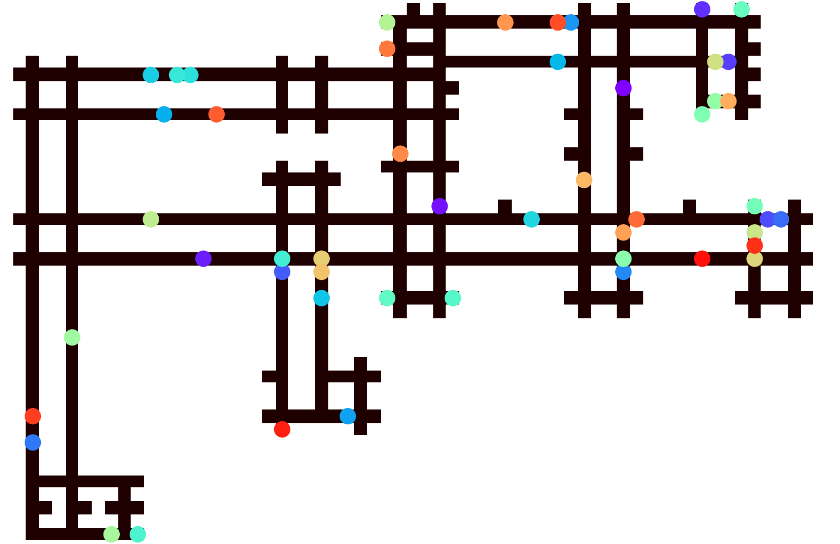
Figure 1: A roadmap occupied by 50 AGVs (represented by colored dots). AGVs must efficiently navigate from a start to a goal position while avoiding collisions with one another, despite being subjected to delays.

Recently, solving the MAPF problem has garnered widespread attention (?; ?). This is mostly due to the abundance of application domains, such as intralogistics, airport taxi scheduling (?) and computer games (?). Solutions to the MAPF problem include Conflict-Based Search (CBS) (?), Prioritized Planning using Safe Interval Path Planning (SIPP) (?), declarative optimization approaches using answer set programming (?), heuristic-guided coordination (?) and graph-flow optimization approaches (?).

Algorithms such as CBS have been improved by exploiting properties such as geometric symmetry (?), using purpose-built heuristics (?), or adopting a Mixed-Integer Linear Program (MILP) formulation where a branch-cut-and-price solver is used to yield significantly faster solution times (?).

Similarly, the development of bounded sub-optimal solvers such as Enhanced Conflict-Based Search (ECBS) (?) have further improved planning performance for higher dimensional state spaces. Continuous Conflict-Based Search (CCBS) can be used to determine MAPF plans for more realistic roadmap layouts (?). As opposed to CBS, CCBS considers a weighted graph and continuous time intervals to describe collision avoidance constraints, albeit with increased solution times.

The abstraction of the MAPF to a graph search problem means that executing the MAPF plans requires monitoring of the assumptions made during the planning stage to ensure and maintain their validity. This is because irregularities such as vehicle dynamics and unpredictable delays influence plan execution. $k$R-MAPF addresses this by permitting delays up to a duration of $k$ time-steps (?). Stochastic AGV delay distributions are considered in (?), where the MAPF is solved by minimizing the expected overall delay. These robust MAPF formulations and solutions inevitably result in more conservative plans compared to their nominal counterparts.

An Action Dependency Graph (ADG)encodes the ordering between AGVs as well as their kinematic constraints in a post-processing step after solving the MAPF (?). Combined with an execution management approach, this allows AGVs to execute MAPF plans successfully despite kinematic constraints and unforeseen delays. This work was extended to allow for persistent re-planning (?).

The aforementioned plan execution solutions in (?; ?; ?) address the effects of delays by ensuring synchronous behavior among AGVs while maintaining the originally planned schedule’s ordering. The result is that plan execution is unnecessarily inefficient when a single AGV is largely delayed and others are on schedule, since AGVs need to wait for the delayed AGV before continuing their plans. We observe that to efficiently mitigate the effects of large delays the plans should be adjusted continuously in an online fashion, where the main challenges are to maintain the original plan’s deadlock- and collision-free guarantees.

In this paper, we present such an online approach capable of reordering AGVs based on a MAPF solution, allowing for efficient MAPF plan execution despite AGVs being subjected to large delays. This approach is fundamentally different from the aforementioned approaches (?; ?; ?; ?) in that delays can be accounted for as they occur, instead of anticipating them a priori. The feedback nature of our approach additionally means solving the initial MAPF can be done assuming nominal plan execution, as opposed to solving a robust formulation which necessarily results in plans of longer length due to the increased conservativeness.

Our contributions include an optimization formulation based on a novel Switchable Action Dependency Graph (SADG)to re-order AGV dependencies. Monte-Carlo simulation results show lower cumulative route completion times with real-time applicable optimization times while guaranteeing collision- and deadlock-free plan execution.

Working towards our proposed solution, we formally define the MAPF problem and the concept of an ADG in Section 2. Based on a modified version of this ADG, we introduce the concept of a reverse agent dependency in Section 3. This will allow an alternative ordering of Automated Guided Vehicles, while maintaining a collision-free schedule. In Section 4, we formulate the choice of selecting between forward or reverse ADG dependencies as a mixed-integer linear programming problem. The optimization problem formulation guarantees that the resulting ADG allows plan execution to be both collision- and deadlock-free, while minimizing the predicted plan completion time. Finally, we compare this approach to the baseline ADG method in Section 5.

2 Preliminaries

Let us now introduce the fundamental concepts on which our approach is based, facilitated by the example shown in Fig. 2. Consider the representation of a workspace by a roadmap $\mathcal{G}=(\mathcal{V},\mathcal{E})$, where $\mathcal{V}$ is a set of vertices and $\mathcal{E}$ a set of edges, e.g., as in Fig. 2(a).

Definition 1 (MAPF Solution).

The roadmap $\mathcal{G}=(\mathcal{V},\mathcal{E})$ is occupied by a set of $N$ AGVs where the $i^{\text{th}}$ AGV has start $s_{i}\in\mathcal{V}$ and goal $g_{i}\in\mathcal{V}$, such that $s_{i}\neq s_{j}$ and $g_{i}\neq g_{j}\;\forall\;i,j\in\{1,\ldots,N\},\;i\neq j$. A MAPF solution $\mathcal{P}=\{\mathcal{P}_{1},\dots,\mathcal{P}_{N}\}$ is a set of $N$ plans, each defined by a sequence $\mathcal{P}=\{p^{1},\dots,p^{N_{i}}\}$ of tuples $p=(l,t)$, with a location $l\in\mathcal{V}$ and a time $t\in[0,\infty)$. The MAPF solution is such that, if every AGV perfectly follows its plan, then all AGVs will reach their respective goals in finite time without collision.

For a plan tuple $p=(l,t)$, let us define the operators $l=loc(p)$ and $t=\hat{t}(p)$ which return the location $l\in\mathcal{V}$ and planned time of plan tuple $p$ respectively. Let $S(l)\mapsto S\subset\mathbb{R}^{2}$ be an operator which maps a location $l$ (obtained from $l=loc(p)$) to a spatial region in the physical workspace in $\mathbb{R}^{2}$. Let $S_{\text{AGV}}\subset\mathbb{R}^{2}$ refer to the physical area occupied by an AGV.

In Fig. 2(a), $AGV_{1}$ and $AGV_{2}$ have start and goal $s_{1}=A$, $g_{1}=H$ and $s_{2}=E$, $g_{2}=D$, respectively. For this example, using CCBS (?) yields $\mathcal{P}=\{\mathcal{P}_{1},\mathcal{P}_{2}\}$ as

• $\mathcal{P}_{1}=\{(A,0),(B,1.0),(C,2.2),(G,3.1),(H,3.9)\}$,

• $\mathcal{P}_{2}=\{(E,0),(F,1.1),(G,3.9),(C,4.8),(D,5.9)\}$.

Note the implicit ordering in $\mathcal{P}$, stating $AGV_{1}$ traverses $C-G$ before $AGV_{2}$.

2.1 Modified Action Dependency Graph

Based on a MAPF solution $\mathcal{P}$, we can construct a modified version of the original Action Dependency Graph (ADG), formally defined in Definition 2. This modified ADG encodes the sequencing of AGV movements to ensure the plans are executed as originally planned despite delays.

Definition 2 (Action Dependency Graph).

An ADG is a directed graph $\mathcal{G}_{\text{ADG}}=(\mathcal{V}_{\text{ADG}},\mathcal{E}_{\text{ADG}})$ where the vertices represent events of an AGV traversing a roadmap $\mathcal{G}$. A vertex $v_{i}^{k}=(\{p_{1},\dots,p_{q}\},\emph{{status}})\in\mathcal{V}_{\text{ADG}}$ denotes the $k^{\text{th}}$ event of the $i^{\text{th}}$ AGV moving from $loc(p_{1})$, via intermediate locations, to $loc(p_{q})$, where $q\geq 2$ denotes the number of consecutive plan tuples encoded within $v_{i}^{k}$. $\emph{{status}}\in\{\emph{{staged}},\emph{{in-progress}},\emph{{completed}}\}$. The edge $(v_{i}^{k},v_{j}^{l})\in\mathcal{E}_{\text{ADG}}$, from here on referred to as a dependency, states that $v_{j}^{l}$ cannot be in-progress or completed until $v_{i}^{k}=\emph{{completed}}$. An edge $(v_{i}^{k},v_{j}^{l})\in\mathcal{E}_{\text{ADG}}$ is classified as Type 1 if $i=j$ and Type 2 if $i\neq j$.

Initially, the status of $v_{i}^{k}$ are $\textit{staged}\;\forall\;i,k$. Let us introduce $plan(v_{i}^{k})$ which returns the sequence of plan tuples $\{p_{1},\dots,p_{q}\}$ for $v_{i}^{k}\in\mathcal{V}_{\text{ADG}}$. Let the operators $s(v_{i}^{k})$ and $g(v_{i}^{k})$ return the start and goal vertices $loc(p_{1})$ and $loc(p_{q})$ of vertex $v_{i}^{k}$ respectively and $\oplus$ denote the Minkowski sum. We also differentiate between planned and actual ADG vertex completion times. Let $\hat{t}_{s}(v_{i}^{k})$ and $\hat{t}_{g}(v_{i}^{k})$ denote the planned time that event $v_{i}^{k}\in\mathcal{V}_{\text{ADG}}$ starts (status changes from staged to in-progress) and is completed (status changes from in-progress to completed), respectively. An ADG can be constructed from a plan $\mathcal{P}$ using Algorithm 1. AGVs can execute their plans as originally described by the MAPF solution $\mathcal{P}$ by adhering to the ADG, defined next in Definition 3.

Definition 3 (Executing ADG based plans).

AGVs adhere to the ADG if each AGV only starts executing an ADG event $v_{i}^{k}$ (status of $v_{i}^{k}$ changes from staged to in-progress) if all dependencies pointing to $v_{i}^{k}$ have status = completed for all $v_{i}^{k}\in\mathcal{V}_{\text{ADG}}$.

Fig. 2(b) shows an example of AGVs adhering to the ADG. Observe how $\lx@glossaries@gls@link{acronym}{AGV}{\leavevmode AGV}_{2}$ cannot start $v_{2}^{2}$ before $v_{1}^{4}$ has been completed by $\lx@glossaries@gls@link{acronym}{AGV}{\leavevmode AGV}_{1}$, as dictated by Definition 3.

Next, we introduce Assumption 1 which we require to maintain deadlock-free behavior between AGVs when executing an ADG based plan as described in Definition 3.

Assumption 1 (Acyclic ADG).

The ADG constructed by Algorithm 1 using $\mathcal{P}$ as defined in Definition 1 is acyclic.

Remark 1.

Assumption 1 can in practice always be satisfied in case the roadmap vertices outnumber the AGV fleet size, i.e. $|\mathcal{V}|>N$ (as is typically the case in warehouse robotics). Simple modificationa to existing MAPF solvers (e.g. an extra edge constraint in CBS) is sufficient to obtain ADG s that satisfy Assumption 1 (?).

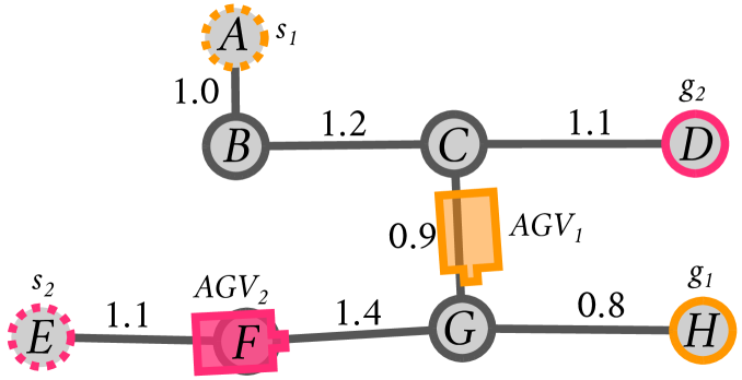
(a) A roadmap graph occupied by two AGVs with start $s_{i}$ and goal $g_{i}$ for $i=\{1,2\}$. The start and goal vertices are highlighted with dotted and solid colored circle outlines respectively. The edge weights indicate the expected traversal times.

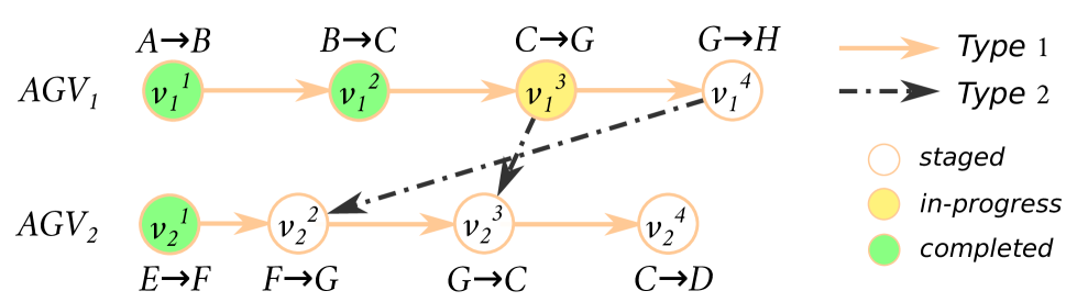
(b) Illustration of the ADG where each vertex status is color coded. It reflects the momentary progress of the AGVs in Fig. 2(a).

Figure 2: Illustrative MAPF problem example alongside the constructed Action Dependency Graph

Algorithm 1 Modified ADG construction based on (?)

0:  MAPF solution $\mathcal{P}=\{\mathcal{P}_{1},\dots,\mathcal{P}_{N}\}$

0:  $\mathcal{G}_{\text{ADG}}$ // Add ADG vertices and Type 1 dependencies

1:  for $i=1$ to $N$ do

2:     $p\leftarrow p_{i}^{1}$

3:     $v\leftarrow(\{p\},staged)$

4:     $v_{\text{prev}}\leftarrow None$

5:     for $k=2$ to $N_{i}$ do

6:        Append $p_{i}^{k}$ to $plan(v)$

7:        if $S(loc(p))\oplus S_{\text{AGV}}\cap S(loc(p_{i}^{k}))\oplus S_{\text{AGV}}=\emptyset$ then

8:           Add $v$ to $\mathcal{V}_{\text{ADG}}$

9:           if $v_{\text{prev}}$ not None then

10:              Add edge $(v_{\text{prev}},v)$ to $\mathcal{E}_{\text{ADG}}$

11:           $v_{\text{prev}}\leftarrow v$

12:           $p\leftarrow p_{i}^{k}$

13:           $v\leftarrow(\{p\},staged)$ // Add Type 2 dependencies

14:  for $i=1$ to $N$ do

15:     for $k=1$ to $N_{i}$ do

16:        for $j=1$ to $N$ do

17:           if $i\neq j$ then

18:              for $l=1$ to $N_{j}$ do

19:                 if $s(v_{i}^{k})=g(v_{j}^{l})$ and $\hat{t}_{g}(v_{i}^{k})\leq\hat{t}_{g}(v_{j}^{l})$ then

20:                    Add edge $(v_{i}^{k},v_{j}^{l})$ to $\mathcal{E}_{\text{ADG}}$

21:  return  $\mathcal{G}_{\text{ADG}}$

Unlike the originally proposed ADG algorithm, Algorithm 1 ensures that non-spatially-exlusive subsequent plan tuples are contained within a single ADG vertex, cf. line 7 of the algorithm. This property will prove to be useful with the introduction of reverse dependencies in Section 3.1. Despite these modifications, Algorithm 1 maintains the original algorithm’s time complexity of $\mathcal{O}(N^{2}\bar{n}^{2})$ where $\bar{n}=\max_{i}N_{i}$.

Due to delays, the planned and actual ADG vertex times may differ. Much like the previously introduced planned event start and completion times $\hat{t}_{s}(v_{i}^{k})$ and $\hat{t}_{g}(v_{i}^{k})$, we also introduce $t_{s}(v_{i}^{k})$ and $t_{g}(v_{i}^{k})$ which denote the actual start and completion times of event $v_{i}^{k}\in\mathcal{V}_{\text{ADG}}$ respectively. Note that if the MAPF solution is executed nominally, i.e. AGVs experience no delays, then $t_{s}(v_{i}^{k})=\hat{t}_{s}(v_{i}^{k})$ and $t_{g}(v_{i}^{k})=\hat{t}_{g}(v_{i}^{k})$ for all $v_{i}^{k}\in\mathcal{V}_{\text{ADG}}$. Let us introduce an important property of an ADG-managed plan-execution scheme, Proposition 1, concerning guarantees of successful plan execution.

Proposition 1 (Collision- and deadlock-free ADG plan execution).

Consider an ADG, $\mathcal{G}_{\text{ADG}}$, constructed from a MAPF solution as defined in Definition 1 using Algorithm 1, satisfying Assumption 1. If the AGV plan execution adheres to the dependencies in $\mathcal{G}_{\text{ADG}}$, then, assuming the AGVs are subjected to a finite number of delays of finite duration, the plan execution will be collision-free and completed in finite time.

Proof 1:

Proof by induction. Consider that $AGV_{i}$ and $AGV_{j}$ traverse a common vertex $\bar{p}\in\mathcal{G}$ along their plans $\mathcal{P}_{i}$ and $\mathcal{P}_{j}$, for any $i,j\in\{1,\dots,N\},i\neq j$. By lines 1-13 of Algorithm 1, this implies $g(v_{i}^{k})=s(v_{j}^{l})=\bar{p}$ for some $v_{i}^{k},v_{j}^{l}\in\mathcal{V}_{\text{ADG}}$. By lines 14-20 of Algorithm 1, common vertices of $\mathcal{P}_{i}$ and $\mathcal{P}_{j}$ in $\mathcal{G}$ will result in a Type 2 dependency $(v_{j}^{l},v_{i}^{k})$ if $p=s(v_{j}^{l})=g(v_{i}^{k})$ and $\hat{t}_{g}(v_{i}^{k})\leq\hat{t}_{g}(v_{j}^{l})$. For the base step: initially, all ADG dependencies have been adhered to since $v_{i}^{1}$ is staged $\forall\;i\in\{1,\dots,N\}$. For the inductive step: assuming vertices up until $v_{i}^{k-1}$ and $v_{j}^{l-1}$ have been completed in accordance with all ADG dependencies, it is sufficient to ensure $AGV_{i}$ and $AGV_{j}$ will not collide at $\bar{p}$ while completing $v_{i}^{k}$ and $v_{j}^{l}$ respectively, by ensuring $t_{s}(v_{i}^{k})>t_{g}(v_{j}^{l})$. By line 19 of Algorithm 1 the Type 2 dependency $(v_{i}^{k},v_{j}^{l})$ guarantees $t_{s}(v_{i}^{k})>t_{g}(v_{j}^{l})$. Since, by Assumption 1, the ADG is acyclic, at least one vertex of the ADG can be in-progress at all times. By the finite nominal execution time of the MAPF solution in Definition 1, despite a finite number of delays of finite duration, finite-time plan completion is established. This completes the proof. $\square$

3 Switching Dependencies in the Action Dependency Graph

We now introduce the concept of a reversed ADG dependency. In the ADG, Type 2 dependencies essentially encode an ordering constraint for AGVs visiting a vertex in $\mathcal{G}$. The idea is to switch this ordering to minimize the effect an unforeseen delay has on the task completion time of each AGV.

3.1 Reverse Type 2 Dependencies

We introduce the notion of a reverse Type 2 dependency in Definition 4. It states that a dependency and its reverse encode the same collision avoidance constraints, but with a reversed AGV ordering. Lemma 1 can be used to obtain a dependency which conforms to Definition 4. Lemma 1 is illustrated graphically in Fig. 3.

Figure 3: A subset of an ADG with a dependency (black) and its reverse (red)

Definition 4 (Reverse Type 2 dependency).

Consider a Type 2 dependency $d=(v_{i}^{k},v_{j}^{l})$. $d$ requires $t_{\text{s}}(v_{j}^{l})\geq t_{g}(v_{i}^{k})$. A reverse dependency of $d$ is a dependency $d^{\prime}$ that ensures $t_{\text{s}}(v_{i}^{k})\geq t_{g}(v_{j}^{l})$.

Lemma 1 (Reversed Type 2 dependency).

Let $v^{k}_{i},v^{l}_{j},v^{l+1}_{j},v^{k-1}_{i}\;\in\mathcal{V}_{\text{ADG}}$. Then $d^{\prime}=(v^{l+1}_{j},v^{k-1}_{i})$ is the reverse dependency of $d=(v^{k}_{i},v^{l}_{j})$.

Proof 2:

The dependency $d=(v^{k}_{i},v^{l}_{j})$ encodes the constraint $t_{s}(v_{j}^{l})\geq t_{g}(v_{i}^{k})$. The reverse of $d$ is denoted as $d^{\prime}=(v^{l+1}_{j},v^{k-1}_{i})$. $d^{\prime}$ encodes the constraint $t_{s}(v_{i}^{k-1})\geq t_{g}(v_{j}^{l+1})$. By definition, $t_{s}(v_{i}^{k})\geq t_{g}(v_{i}^{k-1})$ and $t_{s}(v_{j}^{l+1})\geq t_{g}(v_{j}^{l})$. Since $t_{g}(v)\geq t_{s}(v)$, this implies that $d^{\prime}$ encodes the constraint $t_{s}(v_{i}^{k})\geq t_{g}(v_{j}^{l})$, satisfying Definition 4. $\square$

The modified ADG ensures that reverse dependencies maintain collision avoidance since adjacent vertices in $\mathcal{V}_{\text{ADG}}$ refer to spatially different locations, cf. line 7 in Algorithm 1.

3.2 Switchable Action Dependency Graph

Having introduced reverse Type 2 dependencies, it is necessary to formalize the manner in which we can select dependencies to obtain a resultant ADG. A cyclic ADG implies that two events are mutually dependent, in turn implying a deadlock. To ensure deadlock-free plan execution, it is sufficient to ensure that the selected dependencies result in an acyclic ADG. Additionally, to maintain the collision-avoidance guarantees implied by the original ADG, it is sufficient to select at least one of the forward or reverse dependencies of each forward-reverse dependency pair in the resultant ADG. Since selecting both a forward and reverse dependency always results in a cycle within the ADG, we therefore must either select between the forward or the reverse dependency. To this end, we formally define a Switchable Action Dependency Graph (SADG)in Definition 5 which can be used to obtain the resultant ADG given a selection of forward or reverse dependencies.

Definition 5 (Switchable Action Dependency Graph).

Let an ADG as in Definition 2 contain $m_{T}$ forward-reverse dependency pairs determined using Definition 4. From this ADG we can construct a Switchable Action Dependency Graph $\textit{SADG}(\textbf{{b}}):\{0,1\}^{m_{T}}\to\mathbb{G}$ where $\mathbb{G}$ is the set of all possible ADG graphs obtained by the boolean vector $\textbf{{b}}=\{b_{1},\dots,b_{m_{T}}\}$, where $b_{m}=0$ and $b_{m}=1$ imply selecting the forward and reverse dependency of pair $m$ respectively, for $m\in\{1,\dots,m_{T}\}$.

Corollary 1 (SADG plan execution).

Consider an SADG, $SADG(\textbf{{b}})$, as in Definition 5. If b is chosen such that $\mathcal{G}_{\text{ADG}}$ $=SADG(\textbf{{b}})$ is acyclic, and no dependencies in $\mathcal{G}_{\text{ADG}}$ point from vertices that are staged or in-progress to vertices that are completed, $\mathcal{G}_{\text{ADG}}$ will guarantee collision- and deadlock-free plan execution.

Proof 3:

By definition, any b will guarantee collision-free plans, since at least one dependency of each forward-reverse dependency pair is selected, by Proposition 1. If b ensures $\lx@glossaries@gls@link{acronym}{ADG}{\leavevmode ADG}=\lx@glossaries@gls@link{acronym}{SADG}{\leavevmode SADG}(\textbf{{b}})$ is acyclic, and the resultant ADG has no dependencies pointing from vertices that are staged or in-progress to vertices that are completed, the dependencies within the ADG are not mutually constraining, guaranteeing deadlock-free plan execution.

The challenge is finding b which ensures $\lx@glossaries@gls@link{acronym}{SADG}{\leavevmode SADG}(\textbf{{b}})$ is acyclic, while simultaneously minimizing the cumulative route completion times of the AGV fleet. This is formulated as an optimization problem in Section 4.

4 Optimization-Based Approach

Having introduced the SADG, we now formulate an optimization problem which can be used to determine b such that the resultant ADG is acyclic, while minimizing cumulative AGV route completion times. The result is a Mixed-Integer Linear Program (MILP)which we solve in a closed-loop feedback scheme, since the optimization problem updates the AGV ordering at each iteration based on the delays measured at that time-step.

4.1 Translating a Switchable Action Dependency Graph to Temporal Constraints

Regular ADG Constraints

Let us introduce the optimization variable $t_{i,s}^{k}$ which, once a solution to the optimization problem is determined, will be equal to $t_{s}(v_{i}^{k})$. The same relation applies to the optimization variable $t_{i,g}^{k}$ and $t_{g}(v_{i}^{k})$. The event-based constraints within the SADG can be used in conjunction with a predicted duration of each event to determine when each AGV is expected to complete its plan. Let $\tau(v_{i}^{k})$ be the modeled time it will take $AGV_{i}$ to complete event $v_{i}^{k}\in\mathcal{V}_{\text{ADG}}$ based solely on dynamical constraints, route distance and assuming the AGV is not blocked. For example, we could let $\tau$ equal the roadmap edge length divided by the expected nominal AGV velocity. We can now specify the temporal constraints corresponding to the Type 1 dependencies of the plan of $AGV_{i}$ as

$$\begin{split}t_{i,g}^{1}&\geq t_{i,s}^{1}+\tau(v_{i}^{1}),\\ t_{i,s}^{2}&\geq t_{i,g}^{1},\\ t_{i,g}^{2}&\geq t_{i,s}^{2}+\tau(v_{i}^{2}),\\ t_{i,s}^{3}&\geq t_{i,g}^{2},\\ \vdots\hskip 14.22636pt&\hskip 28.45274pt\vdots\\ t_{i,s}^{N_{i}}&\geq t_{i,g}^{N_{i}-1},\\ t_{i,g}^{N_{i}}&\geq t_{i,s}^{N_{i}}+\tau(v_{i}^{N_{i}}).\end{split}$$ (1)

Consider a Type 2 dependency $(v_{i}^{k},v_{j}^{l})$ within the ADG. This can be represented by the temporal constraint

$$t_{j,s}^{l}>t_{i,g}^{k},$$ (2)

where the strict inequality is required to guarantee that $\lx@glossaries@gls@link{acronym}{AGV}{\leavevmode AGV}_{i}$ and $\lx@glossaries@gls@link{acronym}{AGV}{\leavevmode AGV}_{j}$ never occupy the same spatial region.

Adding Switchable Dependency Constraints

We now introduce the temporal constraints which represent the selection of forward or reverse dependencies in the SADG. Initially, consider the set $\mathcal{E}_{\text{ADG}}^{\text{{Type 2}}}=\{e\in\mathcal{E}_{\text{ADG}}|e\text{ is Type 2}\}$ which represents the sets of all Type 2 dependencies. The aim here is to determine a set $\mathcal{E}_{\text{ADG}}^{\text{switchable}}\subset\mathcal{E}_{\text{ADG}}^{\text{{Type 2}}}$ containing the dependencies which could potentially be switched and form part of the MILP decision space.

Consider $e_{\text{fwd}}=(v_{f},v_{f}^{\prime})\in\mathcal{E}_{\text{ADG}}^{\text{{Type 2}}}$ and its reverse dependency $e_{\text{rev}}=(v_{r},v_{r}^{\prime})$. $e_{\text{fwd}}$ and $e_{\text{rev}}$ are contained within $\mathcal{E}_{\text{ADG}}^{\text{switchable}}$ if the status of $v_{f},v_{f}^{\prime},v_{r},v_{r}^{\prime}$ is staged. An illustrative example of the dependencies contained within $\mathcal{E}_{\text{ADG}}^{\text{switchable}}$ is shown in Fig. 4. Having determined $\mathcal{E}_{\text{ADG}}^{\text{switchable}}$, the next step is to include the switched dependencies as temporal constraints. Directly referring to Section 3.2, we assume $m_{T}$ forward-reverse dependency pairs in $\mathcal{E}_{\text{ADG}}^{\text{switchable}}$, where the Boolean $b_{m}$ is used to select the forward or reverse dependency of the $m$th forward-reverse dependency pair, $m\in\{1,\dots,m_{T}\}$. These temporal constraints can be written as

$$t_{j,s}^{l} >t_{i,g}^{k}-b_{m}M,\;$$ (3)

$$t_{i,s}^{k-1} >t_{j,g}^{l+1}-\big{(}1-b_{m}\big{)}M,\;$$

where $M$ is a large, positive constant such that $M>\max_{i}t_{i}^{N_{i}}$. Note that $\max_{i}t_{i}^{N_{i}}$ can be approximated by estimating the maximum anticipated delays experienced by the AGVs. In practice, however, finding such an upper bound on delays is not evident, meaning we choose $M$ to be a conservatively high value.

4.2 Optimization Problem Formulation

We have shown that an SADG is represented by the temporal constraints in Eq. (1) through Eq. (3) for $i\in\{1,\dots,N\}$, $m\in\{1,\dots,m_{T}\}$. Minimizing the cumulative route completion time of all AGVs is formulated as the following optimization problem

$$\begin{split}\min_{\textbf{{b}},\;\textbf{{t}}_{s},\;\textbf{{t}}_{g}}\hskip 5.69054pt&\sum_{i=1}^{N}t_{i,g}^{N_{i}}\\ \text{s.t. }&Eq.~{}(\ref{eq:type_1_temporal_constraints})\;\forall\;i=\{1,\dots,N\},\\ &Eq.~{}(\ref{eq:type_2_temporal_constraints})\;\forall\;e\in\mathcal{E}_{\text{ADG}}^{\text{{Type 2}}}\setminus\mathcal{E}_{\text{ADG}}^{\text{switchable}},\\ &Eq.~{}(\ref{eq:type_2_switchable_constraints})\;\forall\;e\in\mathcal{E}_{\text{ADG}}^{\text{switchable}},\\ \end{split}$$ (4)

where $\textbf{{b}}:\{0,1\}^{m_{T}}$ is a vector containing all the binary variables $b_{m}$ and the vectors $\textbf{{t}}_{s}$ and $\textbf{{t}}_{g}$ contain all the variables $t_{i,s}^{k}$ and $t_{i,g}^{k}$ respectively $\forall\;k\in\{1,\dots,N_{i}\},i\in\{1,\dots,N\}$.

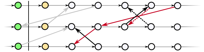
Figure 4: Dependencies contained in $\mathcal{E}_{\text{ADG}}^{\text{switchable}}$, shown in black (forward) and red (reverse). Gray dependencies are in $\mathcal{E}_{\text{ADG}}^{\text{{Type 2}}}\setminus\mathcal{E}_{\text{ADG}}^{\text{switchable}}$.

4.3 Solving the MILP in a Feedback Loop

The aforementioned optimization formulation can be solved based on the current AGV positions in a feedback loop. The result is a continuously updated $\mathcal{G}_{\text{ADG}}$ which guarantees minimal cumulative route completion times based on current AGV delays. This feedback strategy is defined in Algorithm 2.

An important aspect to optimal feedback control strategies is that of recursive feasibility, which means that the optimization problem will remain feasible as long as the control law is applied. The control strategy outlined in Algorithm 2 is guaranteed to remain recursively feasible, as formally shown in Proposition 2.

Algorithm 2 Switching ADG Feedback Scheme

1:  Get goals and locations

2:  Solve MAPF to obtain $\mathcal{P}$

3:  Construct ADG using Algorithm 1

4:  Determine $\text{\lx@glossaries@gls@link{acronym}{SADG}{\leavevmode SADG}}(\textbf{{b}})$ and set $\textbf{{b}}=\textit{{0}}$ (see Section 4.1)

5:  while Plans not done do

6:     get current position along plans for each robot

7:     $\textbf{{b}}\leftarrow$ MILP in Eq. (4)

8:     $\text{\lx@glossaries@gls@link{acronym}{ADG}{\leavevmode ADG}}\leftarrow\text{\lx@glossaries@gls@link{acronym}{SADG}{\leavevmode SADG}}(\textbf{{b}})$

Proposition 2 (Recursive Feasibility).

Consider an ADG, as defined in Definition 2, which is acyclic at time $t=0$. Consecutively applying the MILP solution from Eq. (4) is guaranteed to ensure the resultant ADG remains acyclic for all $t>0$.

Proof 4:

Proof by induction. Consider an acyclic ADG as defined in Definition 2, at a time $t$. The MILP in Eq. (4) always has the feasible solution $\textbf{{b}}=0$ if the initial ADG (from which the MILP’s constraints in Eq. (1) through Eq. (3) are defined) is acyclic. Any improved solution of the MILP with $\textbf{{b}}\neq 0$ is necessarily feasible, implying a resultant acyclic ADG. This implies that the MILP is guaranteed to return a feasible solution, the resultant ADG will always be acyclic if the ADG before the MILP was solved, was acyclic. Since the ADG at $t=0$ is acyclic (a direct result of a MAPF solution), it will remain acyclic for $t>0$. $\square$

4.4 Decreasing Computational Effort

The time required to solve the MILP will directly affect the real-time applicability of this approach. In general, the complexity of the MILP increases exponentially in the number of binary variables. To render the MILP less computationally demanding, it is therefore most effective to decrease the number of binary variables. We present two complementary methods to achieve this goal.

Switching Dependencies in a Receding Horizon

Instead of including all switchable dependency pairs in the set $\mathcal{E}_{\text{ADG}}^{\text{switchable}}$, we can only include the switchable dependencies associated with vertices within a horizon $H$ from the last completed vertex. An illustration of such selection for $H=4$ is shown in Fig. 5. Note that dependency selection using this approach maintains ADG acyclicity as in the infinite horizon case, because the set $\mathcal{E}_{\text{ADG}}^{\text{switchable}}$ is smaller, but Eq. (4) remains recursively feasible since the trivial solution guarantees a acyclic ADG at every time-step. Proposition 2 is equally valid when only considering switchable dependencies in a receding horizon. The horizon length $H$ can be seen as a tuning parameter which can offer a trade-off between computational complexity and solution optimality.

Note that, to guarantee recursive feasibility, any switchable dependencies which are not within the horizon $H$ (e.g. the green dependencies in Fig. 5) still need to be considered within the MILP by applying the constraint in Eq. (2). Future work will look into a receding horizon approach that does not necessarily require the consideration of all these constraints while guaranteeing recursive feasibility.

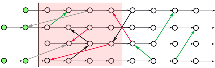
Figure 5: Dependency selection for a horizon of $4$ vertices. Switchable dependency pairs are shown in black (forward) and red (reverse). Regular dependencies considered in the MILP are green. Dependencies not considered are gray.

Dependency Grouping

We observed that multiple dependencies would often form patterns, two of which are shown in Fig. 6. These patterns are referred to as same-direction and opposite-direction dependency groups, shown in Fig. 6(a) and Fig. 6(b) respectively. These groups share the same property that the resultant ADG is acyclic if and only if either all the forward or all the reverse dependencies are active. This means that a single binary variable is sufficient to describe the switching of all the dependencies within the group, decreasing the variable space of the MILP in Eq. (4). Once such a dependency group has been identified, the temporal constraints can then be defined as

$$t_{j,s}^{l} >t_{i,g}^{k}-b_{DG}M\; \forall\;(v_{i}^{k},v_{j}^{l})\in\mathcal{DG}_{\text{fwd}},$$ (5)

$$t_{j,s}^{l} >t_{i,g}^{k}-(1-b_{DG})M\;\; \forall\;(v_{i}^{k},v_{j}^{l})\in\mathcal{DG}_{\text{rev}},$$

where $\mathcal{DG}_{\text{fwd}}$ and $\mathcal{DG}_{\text{rev}}$ refer to the forward and reverse dependencies of a particular grouping respectively, and $b_{DG}$ is a binary variable which switches all the forward or reverse dependencies in the entire group simultaneously.

(a) same

(b) opposite

Figure 6: Dependency groups. Each dependency is either original (black) or reversed (red). Reverse and forward dependency pairings are differentiated by line styles.

5 Evaluation

We design a set of simulations to evaluate the approach in terms of re-ordering efficiency when AGVs are subjected to delays while following their initially planned paths. We use the method presented by Hönig et al. (?) as a comparison baseline. All simulations were conducted on a Lenovo Thinkstation with an Intel® Xeon E5-1620 3.5GHz processor and 64 GB of RAM.

5.1 Simulation Setup

The simulations consider a roadmap as shown in Fig. 1. A team of AGVs of size $\{30,40,50,60,70\}$ are each initialized with a random start and goal position. ECBS (?) is used to solve the MAPF with sub-optimality factor $w=1.6$. We consider delays of duration $k=\{1,3,5,10,15,20,25\}$ time-steps. At the $k^{th}$ time-step, a random subset (20%) of the AGVs are stopped for a length of $k$. Eq. (4) is solved at each time-step with $M=10^{4}$. We evaluate our approach using a Monte Carlo method: for each AGV team size and delay duration configuration, we consider $100$ different randomly selected goal/start positions. The receding horizon dependency selection and dependency groups are used as described in Section 4.4.

5.2 Performance Metric and Comparison

Performance is measured by considering the cumulative plan completion time of all the AGVs. This is compared to the same metric using the original ADG approach with no switching as in (?), which is equivalent to forcing the solution of Eq. (4) to $\textbf{{b}}=\textbf{0}$ at every time-step. The improvement is defined as

$$\text{improvement}=\frac{\sum t_{\text{baseline}}-\sum t_{\text{switching}}}{\sum t_{\text{baseline}}}\cdot 100\%,$$

where $\sum t_{\ast}$ refers to the cumulative plan completion time for all AGVs. Note that we consider cumulative plan completion time instead of the make-span because we want to ensure each AGV completes its plans as soon as possible, such that it can be assigned a new task.

Another important consideration is the time it takes to solve the MILP in Eq. (4) at each time-step. For our simulations, the MILP was solved using the academically orientated Coin-Or Branch-and-Cut (CBC) solver (?). However, based on preliminary tests, we did note better performance using the commercial solver Gurobi (?). This yielded computational time improvements by a factor 1.1 up to 20.

5.3 Results and Discussion

To showcase the efficacy of our approach, we first determine the average improvement of $100$ random scenarios using the minimum switching horizon length of $1$ for different AGV team sizes and delay lengths, shown in Fig. 7. The average improvement is highly correlated to the delay duration experienced by the AGVs.

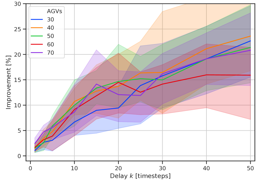
Figure 7: Average improvement of $100$ scenarios for various delay lengths and AGV group sizes. Each scenario refers to different randomly generated starts/goals and a randomly selected subset of delayed AGVs. Solid lines depict the average, lighter regions encapsulate the min-max values.

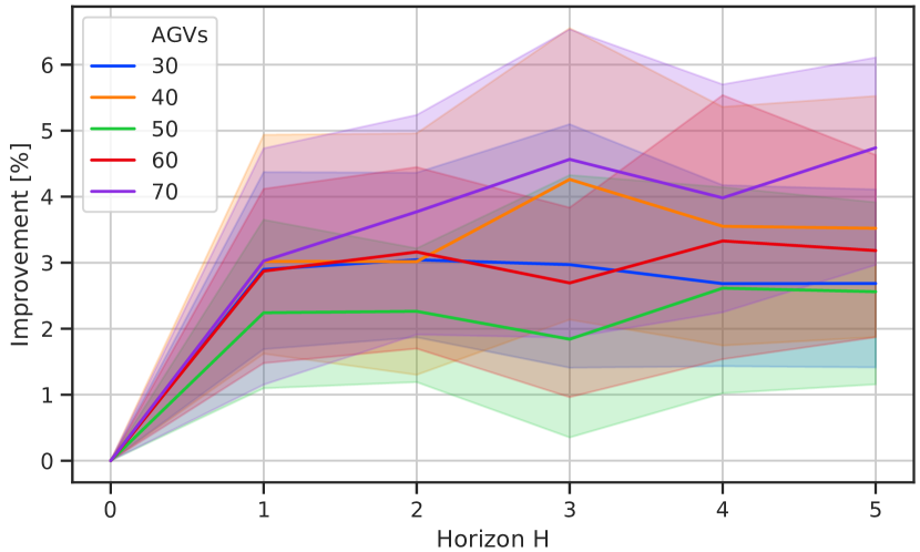
(a) Delay $k=3$.

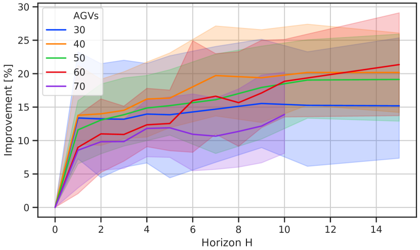
(b) Delay $k=25$.

Figure 8: Average improvement of $100$ random start/goal positions and delayed AGV subset, for different switching horizon lengths, for different AGV group sizes. Solid lines depict the average, lighter regions encapsulate the min-max values.

Considering Fig. 7, it is worth noting how the graph layout and AGV-to-roadmap density affects the results: the AGV group size of $40$ shows the best average improvement for a given delay duration. This leads the authors to believe there is an optimal AGV group size for a given roadmap, which ensures the workspace is both:

1. Not too congested to make switching of dependencies impossible due to the high density of AGVs occupying the map.

2. Not too sparse such that switching is never needed since AGVs are distant from each other, meaning that switching rarely improves task completion time.

Considering the switching dependency horizon, Fig. 8 shows the average improvement for $100$ random start/goal positions and delayed AGV subset selection. We observe that a horizon length of $1$ already significantly improves performance, and larger horizons seem to gradually increase performance for larger AGV teams.

Fig. 9 shows the peak computation time for various horizon lengths and AGV team sizes. As expected, the computation time is exponential with horizon size and AGV team size.

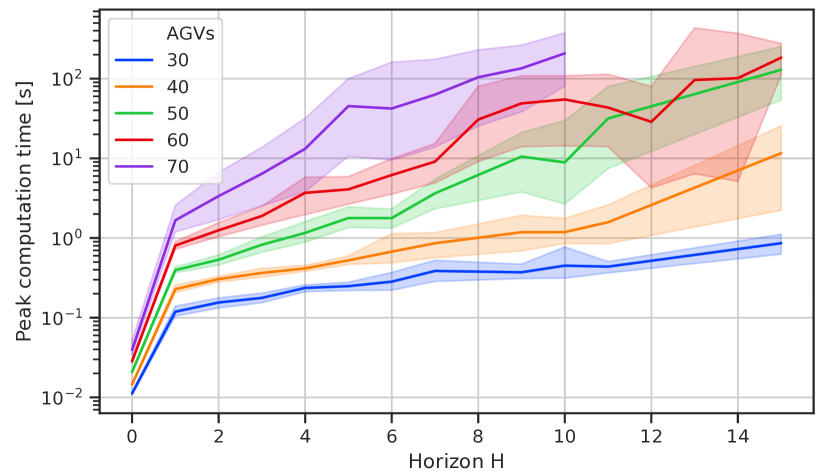
Figure 9: The peak computation to solve the optimization problem for different AGV team sizes and considered dependency horizon lengths. This plot considers the average improvement for delays $k=\{1,3,5,10,15,20,25\}$. Solid lines depict the average, lighter regions encapsulate the min-max values.

Two additional observations that were made:

1. High variability in results. Note the high variability in improvement indicated by the large lighter regions in Fig. 7. This means that for different random start/goal and delay configurations, the improvement varied significantly. This is due to the fact that each start/goal combination provides differing degrees-of-freedom from an ADG switching perspective.

2. Occasional worse performance. Occasionally, albeit rarely, our approach would yield a negative improvement for a particular random start/goal configuration. This was typically observed for small delay durations. The reason is that the optimization problem solves the switching assuming no future delays. However, it may so happen that the AGV which was allowed ahead of another, is delayed in the near future, additionally delaying the AGV it surpassed. We believe a robust optimization approach could potentially resolve this.

Finally, we emphasize that our proposed approach:

1. Is a complementary approach which could be used together with the methods presented in (?; ?) and other works.

2. Applies to directional and weighted roadmaps (since ADG switching retains the direction of the original MAPF plan);

3. Persistent planning schemes as in (?), as long as all AGV plans $\mathcal{P}$ are known when the ADG is constructed.

6 Conclusions and Future Work

In this paper, we introduced a novel method which, given a MAPF solution, can be used to switch the ordering of AGVs in an online fashion based on currently measured AGV delays. This switching was formulated as an optimization problem as part of a feedback control scheme, while maintaining the deadlock- and collision-free guarantees of the original MAPF plan. Results show that our approach clearly improves the cumulative task completion time of the AGVs when a subset of AGVs are subjected to delays.

In future work, we plan to consider a receding horizon optimization approach. In this work, ADG dependencies can be switched in a receding horizon fashion, but the plans still need to be of finite length for the optimization problem to be formulated. For truly persistent plans (theoretically infinite length plans), it is necessary to come up with a receding horizon optimization formulation to apply the method proposed in this paper.

Another possible extension is complementing our approach with a local re-planning method. This is because our approach maintains the originally planned trajectories of the AGVs. However, we observed that under large delays, the originally planned routes can become largely inefficient due to the fact the AGVs are in entirely different locations along their planned path. This could potentially be addressed by introducing local re-planning of trajectories.

To avoid the occasional worse performance, we suggest a robust optimization approach to avoid switching dependencies which could have a negative impact on the plan execution given expected future delays.

Finally, to further validate this approach, it is desirable to move towards system-level tests on a real-world intralogistics setup.

References

- [Andreychuk et al. 2019] Andreychuk, A.; Yakovlev, K.; Atzmon, D.; and Stern, R. 2019. Multi-agent pathfinding with continuous time. In Proceedings of the Twenty-Eighth International Joint Conference on Artificial Intelligence, IJCAI-19, 39–45. International Joint Conferences on Artificial Intelligence Organization.
- [Atzmon et al. 2020] Atzmon, D.; Stern, R.; Felner, A.; Wagner, G.; Barták, R.; and Zhou, N.-F. 2020. Robust Multi-Agent Path Finding and Executing. Journal of Artificial Intelligence Research 67:549–579.
- [Barer et al. 2014] Barer, M.; Sharon, G.; Stern, R.; and Felner, A. 2014. Suboptimal variants of the conflict-based search algorithm for the multi-agent pathfinding problem. In Proceedings of the European Conference on Artificial Intelligence (ECAI), 961–962.
- [Bogatarkan, Patoglu, and Erdem 2019] Bogatarkan, A.; Patoglu, V.; and Erdem, E. 2019. A declarative method for dynamic multi-agent path finding. In Calvanese, D., and Iocchi, L., eds., GCAI 2019. Proceedings of the 5th Global Conference on Artificial Intelligence, volume 65 of EPiC Series in Computing, 54–67. EasyChair.
- [Felner et al. 2017] Felner, A.; Stern, R.; Shimony, S. E.; Boyarski, E.; Goldenberg, M.; Sharon, G.; Sturtevant, N. R.; Wagner, G.; and Surynek, P. 2017. Search-based optimal solvers for the multi-agent pathfinding problem: Summary and challenges. In Fukunaga, A., and Kishimoto, A., eds., Proceedings of the Tenth International Symposium on Combinatorial Search, SOCS 2017, 16-17 June 2017, Pittsburgh, Pennsylvania, USA, 29–37. AAAI Press.
- [Felner et al. 2018] Felner, A.; Li, J.; Boyarski, E.; Ma, H.; Cohen, L.; Kumar, S.; and Koenig, S. 2018. Adding heuristics to conflict-based search for multi-agent path finding. In Proceedings of the International Conference on Automated Planning and Scheduling (ICAPS), 83–87.
- [Forrest et al. 2018] Forrest, J.; Ralphs, T.; Vigerske, S.; LouHafer; Kristjansson, B.; jpfasano; EdwinStraver; Lubin, M.; Santos, H. G.; rlougee; and Saltzman, M. 2018. coin-or/cbc: Version 2.9.9.
- [Gurobi Optimization, LLC 2020] Gurobi Optimization, LLC. 2020. Gurobi optimizer reference manual.
- [Hönig et al. 2017] Hönig, W.; Kumar, S.; Cohen, L.; Ma, H.; Xu, H.; Ayanian, N.; and Koenig, S. 2017. Summary: Multi-agent path finding with kinematic constraints. In Proceedings of the International Joint Conference on Artificial Intelligence (IJCAI), 4869–4873.
- [Hönig et al. 2019] Hönig, W.; Kiesel, S.; Tinka, A.; Durham, J.; and Ayanian, N. 2019. Persistent and robust execution of MAPF schedules in warehouses. IEEE Robotics and Automation Letters 4(2):1125–1131.
- [Lam et al. 2019] Lam, E.; Bodic, P. L.; Harabor, D.; and Stuckey, P. 2019. Branch-and-cut-and-price for multi-agent pathfinding. In Proceedings of the International Joint Conference on Artificial Intelligence (IJCAI), (in print).
- [Li et al. 2019] Li, J.; Harabor, D.; Stuckey, P.; Ma, H.; and Koenig, S. 2019. Symmetry-breaking constraints for grid-based multi-agent path finding. In Proceedings of the AAAI Conference on Artificial Intelligence (AAAI), (in print).
- [Ma, Kumar, and Koenig 2017] Ma, H.; Kumar, S.; and Koenig, S. 2017. Multi-agent path finding with delay probabilities. In Proceedings of the AAAI Conference on Artificial Intelligence (AAAI), 3605–3612.
- [Morris et al. 2016] Morris, R.; Pasareanu, C. S.; Luckow, K. S.; Malik, W.; Ma, H.; Kumar, T. K. S.; and Koenig, S. 2016. Planning, scheduling and monitoring for airport surface operations. In AAAI Workshop: Planning for Hybrid Systems.
- [Ontanón et al. 2013] Ontanón, S.; Synnaeve, G.; Uriarte, A.; Richoux, F.; Churchill, D.; and Preuss, M. 2013. A survey of real-time strategy game ai research and competition in starcraft. IEEE Transactions on Computational Intelligence and AI in games 5(4):293–311.
- [Pecora et al. 2018] Pecora, F.; Andreasson, H.; Mansouri, M.; and Petkov, V. 2018. A loosely-coupled approach for multi-robot coordination, motion planning and control. In Twenty-eighth international conference on automated planning and scheduling.
- [Sharon et al. 2015] Sharon, G.; Stern, R.; Felner, A.; and Sturtevant, N. R. 2015. Conflict-based search for optimal multi-agent pathfinding. Artificial Intelligence 219:40 – 66.
- [Stern et al. 2019] Stern, R.; Sturtevant, N.; Felner, A.; Koenig, S.; Ma, H.; Walker, T. T.; Li, J.; Atzmon, D.; Cohen, L.; Kumar, T. K. S.; Boyarski, E.; and Barták, R. 2019. Multi-agent pathfinding: Definitions, variants, and benchmarks. CoRR abs/1906.08291.
- [Wurman, D’Andrea, and Mountz 2008] Wurman, P. R.; D’Andrea, R.; and Mountz, M. 2008. Coordinating hundreds of cooperative, autonomous vehicles in warehouses. volume 29 of AI Magazine, 9 – 19. Menlo Park, CA: AAAI.
- [Yakovlev and Andreychuk 2017] Yakovlev, K. S., and Andreychuk, A. 2017. Any-angle pathfinding for multiple agents based on SIPP algorithm. CoRR abs/1703.04159.
- [Yu and LaValle 2012] Yu, J., and LaValle, S. M. 2012. Multi-agent Path Planning and Network Flow. CoRR abs/1204.5717.
- [Yu and LaValle 2013] Yu, J., and LaValle, S. M. 2013. Planning optimal paths for multiple robots on graphs. In 2013 IEEE International Conference on Robotics and Automation, 3612–3617.