Model Identification and Adaptive State Observation for a Class of Nonlinear Systems

Abstract

In this paper we consider the joint problems of state estimation and model identification for a class of continuous-time nonlinear systems in output-feedback canonical form. An adaptive observer is proposed that combines an extended high-gain observer and a discrete-time identifier. The extended observer provides the identifier with a data set permitting the identification of the system model and the identifier adapts the extended observer according to the new estimated model. The design of the identifier is approached as a system identification problem and sufficient conditions are presented that, if satisfied, allow different identification algorithms to be used for the adaptation phase. The cases of recursive least-squares and multiresolution black-box identification via wavelet-based identifiers are specifically addressed. Stability results are provided relating the asymptotic estimation error to the prediction capabilities of the identifier. Robustness with respect to additive disturbances affecting the system equations and measurements is also established in terms of an input-to-state stability property relative to the noiseless estimates.

I Introduction

I-A Problem Description and Literature Overview

We consider nonlinear systems of the form

$$\begin{array}[]{lclr}\dot{x}_{i}&=&x_{i+1}+d_{i}&\quad i=1,\dots,n-1\\ \dot{x}_{n}&=&\phi(x)+d_{n}\\ y&=&x_{1}+\nu\end{array}$$ (1)

where $x=(x_{1},\dots,x_{n})\in\mathbb{R}^{{n{p}}}$, $x_{i}\in\mathbb{R}^{p}$, is the state, $y\in\mathbb{R}^{p}$ is the measured output, $d:=\operatorname{col}(d_{1},\dots,d_{n})\in\mathbb{R}^{{n{p}}}$ and $\nu\in\mathbb{R}^{p}$ are unknown disturbances, and $\phi:\mathbb{R}^{{n{p}}}\to\mathbb{R}^{p}$ is a function unknown to the designer and fulfilling technical assumptions specified later. For the class of systems (1), in this paper we consider the problem of designing an adaptive observer that, when the disturbances $d$ and $\nu$ are not present, produces asymptotically “good” estimates of both the system state $x$ and the system model $\phi$, and that, when instead $d$ and $\nu$ are present, guarantees a corresponding “input-to-state stability” property relative to such asymptotic estimates. An adaptive observer with those properties is called in [1] a robust adaptive observer.

State estimation is a problem of primary interest in control, and its applications are ubiquitous in all the related engineering areas. Having available good models, on the other hand, is of crucial importance in many contexts, as for instance in model predictive control [2] and control in presence of delays [3], where models are used to cast predictions, in tracking and output regulation [4], in which they are used to model the exogenous references or disturbances acting on the system, and in signal processing and the related applications [5, 6], in which models are used to extract information about the surrounding environment and to detect events. In this paper we jointly consider both the problems of estimating the system state $x$ and its model $\phi$.

The problem of designing adaptive observers for uncertain nonlinear systems boasts decades of active research, and it constitutes nowadays an important branch of adaptive control. The class of systems (1), in turn, is among the most studied, and the many contributions developed in the years mainly differ in terms of the hypotheses on the structure of the uncertain model here represented by $\phi$. Systems in which the uncertainty is concentrated in a set of parameters entering linearly in the model have been considered for instance in [7, 8, 9] and [1], where in the latter work also robustness with respect to additive disturbances (modeled by $d$ in (1)) is proved. Related extensions to multivariable systems and more general forms appeared in [10, 11] in a disturbance-free setting. Adaptive observers for models admitting nonlinear parametrizations in the uncertain parameters started to appear in more recent times (see [12, 13, 14, 15] and the references therein). In particular, in [12] a general class of high-gain observers is endowed with an adaptation mechanism of the kind of that proposed in [11]. In [13], a fairly more general class of nonlinear parametrizations is considered for uniformly observable systems, where also robustness with respect to disturbances $d$ affecting the system dynamics is shown to hold. In [14], the theory of nonlinear Luenberger observers [16] is applied to estimate the state and parameters of uncertain linear systems and, in [15], more general systems exhibiting nonlinearities in both the states and the parameters are dealt with by using the same arguments of [17] in dealing with non-uniformly observable systems.

Most of the existing approaches are strongly based on a canonical “adaptive control” perspective, in which all the uncertainty is concentrated in a set of parameters with known dimension, whose knowledge would result in the knowledge of the true system to be observed. In line with the certainty equivalence principle, uncertainty is usually dealt with by using an estimate of the true uncertain parameter, whose adaptation is carried out by ad hoc adaptation laws induced by Lyapunov analysis or immersion arguments. While for linear systems parametric perturbations do actually exhaust the kind of model uncertainties we may care about, this is definitely not the case for nonlinear systems, where limiting to parametric perturbations means considering variations of functions in quite “restricting” topologies [18]. Furthermore, the assumption of a known parametrization is also not robust relative to quite standard topologies, in the sense that even if a nominal model admits the supposed parametrization, any arbitrarily “small” neighborhood of the nominal model will contain functions not having such a structure. This, indeed, makes the approaches constructed around the notion of a “true model” conceptually fragile, especially in view of the fact that robustness to disturbances is usually not shown. In particular, among the aforementioned approaches, only [1], [13] and [14] consider robustness to disturbances affecting the system dynamics ($d$ in (1)), and only [14] considers also measurement noise ($\nu$ in (1)). The result of [14], however, limits to linear systems, and the robustness property is in general only local in both $d$ and $\nu$, and can be made global only under some additional boundedness conditions on the parametrization.

I-B Objectives, Results and Organization of the Paper

The main goal of this paper is to propose a class of robust adaptive observers estimating both the state and the model of system (1), and whose construction is not tailored around the assumption of a known structure of the system’s model $\phi$ and does not necessarily rely on the existence of a “true model” and of a corresponding “true parameter” to estimate. Instead, we aim to approach model estimation as a system identification problem [19], with the goal of connecting the quality of the state and model estimation to the prediction performance of the employed identification scheme. The quest of estimating the true parameter is thus substituted with that of finding the best model possible and, accordingly, the objective of asymptotic state estimation is substituted by a weaker optimality property of the identified model, more likely achievable robustly. In this way, we aim at opening the doors to nonlinear black-box techniques and universal approximators [20, 21], by adopting, however, standard analysis tools typical of systems and control theory.

System identification is a very rich and developed research area, and an enormous variety of techniques and algorithms exist whose applicability strongly depends on the kind of signals under concern. Consistently with the aforementioned objective, we do not intend here to focus on a single identification algorithm, that would inexorably make sense only for a restricted class of models of $\phi$. Rather we aim to extract and provide generic sufficient conditions that an arbitrary identification algorithm must satisfy to be used in the framework, while leaving to the user the choice of the particular strategy to employ depending on the a priori qualitative information available on the system. In these terms, we seek a solution which is modular in the choice of the adaptation strategy and, thus, which can be adapted to the particular application context and to the amount and quality of the a priori information that the designer has on the system.

To this end, we endow an extended high-gain observer with a generic discrete-time identifier satisfying some steady-state optimality and strong stability assumptions detailed later. The extended observer provides the identifier with a “dirty” data set that the identifier can use to extract information about the system model $\phi$. The identifier adapts the extended observer according to its best guess of $\phi$, thus increasing the observer performance. The main result of the paper is an approximate estimation result stating that the adaptive observer produces an estimate of the system state and model that is asymptotically bounded by the “size” of the disturbances $d$ and $\nu$, and by the prediction capabilities of the chosen identifier.

The paper is organized as follows. In Section II we present the adaptive observer; in Section III we give the main result; in Section IV, we show how an identifier implementing the well-known recursive least-squares scheme can be constructed, and based on that, we propose a recursive identifier performing a black-box identification procedure based on wavelet and multiresolution analysis. Finally in Section V we present some examples.

I-C Contribution of the Paper

State estimation for systems of the form (1) in presence of uncertain $\phi$, alone, is a problem that does not actually need adaptation to give acceptable results when single experiments are concerned. As a matter of fact, in a noise-free context, standard high-gain observers can be used to obtain a practical state estimate without knowing $\phi$ exactly [22], or sliding-mode and homogeneous observers can be used to get a theoretically asymptotic estimate by just knowing a bound on $\phi(x)$ [23, 24]. The use of adaptation, in turn, is typically motivated when also the model of the observed system is needed other than its state, or when one is interested to obtain an observer that is actually able to generate the trajectories of the observed system. The main contribution of this paper concerns this latter cases, where it intersects the already vast literature on adaptive observation. Compared to the existing approaches, in this paper adaptation is treated in more general terms as a system identification problem, and the proposed solution is modular in the choice of the adaptation strategy, thus allowing the user to employ different techniques depending on the actual needs. This, in turn, requires a different approach to the analysis and synthesis that is based on a logical separation of the roles of the observer and the identifier. Furthermore, the proposed design is intrinsically robust to measurement noise and additive disturbances, without the need of introducing tedious modifications of the adaptive strategy or the observer.

Regarding the actual design of identifiers, as a particular case we show that the well-known least-squares schemes fit into the framework, and we propose a novel black-box identifier performing a wavelet multiresolution approximation of arbitrary $L^{2}$ functions.

The observer is specifically designed to support discrete-time identifiers. This is motivated by the fact that system identification approaches are usually discrete-time. Their use, however, comes with the price of a considerable technical overhead, requiring to study the overall interconnection in the formal context of hybrid dynamical systems [25].

I-D Notation

We denote by $\mathbb{R}$, $\mathbb{N}$ and $\mathbb{Z}$ the set of real, natural and integer numbers, and we let $\mathbb{R}_{+}:=[0,\infty)$. If $S$ is a set, $\operatorname{card}{S}$ denotes its cardinality. We denote by $|\cdot|$ any norm whenever the underlying normed space is clear. If $S$ a subset of a normed vector space $\mathcal{X}$ and $x\in\mathcal{X}$, we let $|x|_{S}:=\inf_{s\in S}|x-s|$. With $A_{1},\dots,A_{n}$ matrices, we denote by $\operatorname{col}(A_{1},\dots,A_{n})$ and $\operatorname{diag}(A_{1},\dots,A_{n})$ their column and diagonal concatenations. For an indexed family of matrices $\{A_{b}\}_{b\in\mathcal{B}}$, we also use the notation $\operatorname{col}(A_{b}\,\mid\,b\in\mathcal{B})$. We denote by $\operatorname{msv}(A)$ the minimum non-zero singular value of the matrix $A$. A function $\gamma:\mathbb{R}_{+}\to\mathbb{R}_{+}$ belongs to class-$\mathcal{K}$ ($\gamma\in\mathcal{K}$) if it is continuous, strictly increasing and $\gamma(0)=0$. If moreover $\gamma(s)\to_{s\to\infty}\infty$, $\gamma$ is said to belong to class-$\mathcal{K}_{\infty}$ ($\gamma\in\mathcal{K}_{\infty}$). A continuous function $\beta:\mathbb{R}_{+}\times\mathbb{R}_{+}\to\mathbb{R}_{+}$ belongs to class-$\mathcal{K}\mathcal{L}$ ($\beta\in\mathcal{K}\mathcal{L}$) if for each $t\in\mathbb{R}_{+}$, $\beta(\cdot,t)\in\mathcal{K}$ and for each $s\in\mathbb{R}_{+}$, $\beta(s,\cdot)$ is decreasing and $\beta(s,t)\to_{t\to\infty}0$. For $k\in\mathbb{N}$, $\mathcal{C}^{k}$ denotes the set of $k$-times continuously differentiable functions. If $\phi$ is a function, $\operatorname{supp}\phi$ denotes its support. $L^{2}(\mathcal{X})$ denotes the Lebesgue space of square integrable functions $\mathcal{X}\to\mathbb{R}$. We denote by $\langle\cdot,\cdot\rangle$ the usual scalar product on $L^{2}(\mathcal{X})$ and we equip $L^{2}(\mathcal{X})$ with the norm $|\cdot|:=\sqrt{\langle\cdot,\cdot\rangle}$.

In this paper we deal with hybrid systems, which are dynamical systems whose state may exhibit both a continuous-time evolution and impulsive changes. Hybrid systems are formally described by equations of the form [25]

$$\Sigma:\left\{\begin{array}[]{lclrl}\dot{x}&=&F(x,u)&&(x,u)\in C\\ x^{+}&=&G(x,u)&&(x,u)\in D\end{array}\right.$$ (2)

where $x$ denotes the state, $u$ an exogenous input, and $C$ and $D$ denote the sets in which continuous and discrete-time dynamics are allowed. In particular, the first equation of (2) means that the state can evolve according to $\dot{x}=F(x,u)$ whenever $(x,u)\in C$. The second equation means that the state can exhibit an impulsive change, from $x$ to $G(x,u)$, whenever $(x,u)\in D$. The solutions of (2) are defined over hybrid time domains, which generalize the usual time domains $\mathbb{R}_{+}$ and $\mathbb{N}$ of continuous and discrete time systems. In particular, a compact hybrid time domain is a subset of $\mathbb{R}_{+}\times\mathbb{N}$ of the form $\mathcal{T}=\cup_{j=0}^{J-1}[t_{j},t_{j+1}]\times\{j\}$ for some $J\in\mathbb{N}$ and $0=t_{0}\leq t_{1}\leq\dots\leq t_{J}$. A set $\mathcal{T}\subset\mathbb{R}_{+}\times\mathbb{N}$ is called a hybrid time domain if for each $(T,J)\in\mathbb{R}_{+}\times\mathbb{N}$, $\mathcal{T}\cap[0,T]\times\{1,\dots,J\}$ is a compact hybrid time domain. For $(t,j),(s,i)\in\mathcal{T}$, we write $(t,j)\preceq(s,i)$ if $t+j\leq s+i$, we let $t^{j}=\sup_{t\in\mathbb{R}}(t,j)\in\mathcal{T}$, $t_{j}:=\inf_{t\in\mathbb{R}}(t,j)\in\mathcal{T}$ and we define $j_{t}$ and $j^{t}$ similarly.

A function $x:\mathcal{T}\to\mathcal{X}$ defined on a hybrid time domain $\mathcal{T}$ is called a hybrid arc if $x(\cdot,j)$ is locally absolutely continuous for each $j$. Hybrid arcs define the space in which the solutions of (2) live, and they play the same role of absolutely continuous signals in a standard continuous-time setting. Further restrictions are needed for a hybrid arc to be used as input in (2). In particular, a hybrid input $u$ is a hybrid arc such that $u(\cdot,j)$ is locally essentially bounded and Lebesgue measurable for each $j$. A pair $(x,u)$ is called a solution pair to (2) if $x$ is a hybrid arc, $u$ is a hybrid input, and $(x,u)$ satisfy (2). We call a solution pair complete if its time domain is unbounded. We let $\operatorname{dom}x$ denote the domain of $x$, $\operatorname{Flw}x\subset\mathbb{R}_{+}$ the set of $t$ such that $(t,j)\in\operatorname{dom}x$ for some $j\in\mathbb{N}$, and $\operatorname{Jmp}x\subset\mathbb{N}$ the set of $j$ such that $(t,j)\in\operatorname{dom}x$ for some $t\in\mathbb{R}$. In order to simplify the notation, we omit the jump (resp. flow) equation when the considered system has only continuous-time (resp. discrete-time) dynamics. If $x$ is constant during flows (resp. jumps), we neglect the “$t$” (resp “$j$”) argument and we write $x(j)$ (resp $x(t)$), which we identify with the map $\operatorname{Jmp}x\ni j\mapsto x(t_{j},j)$ (resp $\operatorname{Flw}x\ni t\mapsto x(t,j_{t})$). We say that a hybrid arc $x$ is eventually in a set $X$ if for some $s\in\operatorname{dom}x$, $x(t,j)\in X$ for all $(t,j)\succeq s$. With $u:\operatorname{dom}u\to\mathcal{U}$ a hybrid input, and $\Gamma(u):=\{(t,j)\in\operatorname{dom}u\,\mid\,(t,j+1)\in\operatorname{dom}u\}$, for $(t,j)\in\operatorname{dom}u$ we let $|u|_{(t,j)}:=\max\{\sup_{(t,j)\in\Gamma(u),\,(0,0)\preceq(s,i)\preceq(t,j)}|u(s,i)|,\allowbreak\mskip 0.0mu plus 0.5mu\operatorname{ess.sup}_{(s,i)\in\operatorname{dom}u/\Gamma(u),(0,0)\preceq(s,i)\preceq(t,j)}|u(s,i)|\}$. If $u$ is constant during jumps (resp. flows), we write $|u|_{t}$ (resp $|u|_{j}$) as short for $|u|_{(t,j)}$. We also let $|u|_{A,(t,j)}:=\big{|}|u|_{A}\big{|}_{(t,j)}$ and $|u|_{\infty}:=\limsup_{t+j\to\infty,(t,j)\in\operatorname{dom}u}|u|_{(t,j)}$. Given a hybrid arc $x$ we will abbreviate $\limsup_{t+j\to\infty,(t,j)\in\operatorname{dom}x}x(t,j)$ with $\limsup_{t+j\to\infty}x$. A collection of hybrid arcs $\mathcal{H}$ is “eventually equibounded” if there exist $\tau,m>0$ such that $|x(t,j)|\leq m$ for each $x\in\mathcal{H}$ and $(t,j)\in\operatorname{dom}x$ satisfying $t+j\geq\tau$. The abbreviation “ISS” stands for “input-to-state stability”.

II The Adaptive Observer

System (1) can be written in compact form as

$$\begin{array}[]{lcl}\dot{x}&=&Ax+B\phi(x)+d\\ y&=&Cx+\nu\end{array}$$ (3)

with

$$A :=\begin{pmatrix}0_{({n{p}}-{p})\times{p}}&I_{{n{p}}-{p}}\\ 0_{p}&0_{{p}\times({n{p}}-{p})}\end{pmatrix}, B :=\begin{pmatrix}0_{({n{p}}-{p})\times{p}}\\ I_{p}\end{pmatrix}$$

$$C :=\begin{pmatrix}I_{p}&0_{{p}\times({n{p}}-{p})}\end{pmatrix}.$$

On system (3) we make the following assumption.

Assumption 1.

The function $\phi$ is locally Lipschitz. Moreover, $d$ and $\nu$ are hybrid inputs and there exist (known) compact sets $\mathcal{X}_{0}\subset\mathcal{X}\subset\mathbb{R}^{n{p}}$ and, for each $x_{0}\in\mathcal{X}_{0}$, a set $\mathbb{D}(x_{0})$ of hybrid inputs with values in $\mathbb{R}^{n{p}}$, such that each solution pair $(x,d)$ to (3) with $x(0)\in\mathcal{X}_{0}$ and $d\in\mathbb{D}(x(0))$ satisfies $x(t)\in\mathcal{X}$ for all $t\in\operatorname{dom}x$.

Remark 1.

Assumption 1 is a boundedness condition requiring the solutions to (3) originating inside a known, arbitrary compact set $\mathcal{X}_{0}$ to be uniformly bounded. Since the effect of $d$ on the time evolution of $x$ depends on the value of $\phi$, then Assumption 1 imposes a joint restriction on $\phi$ and the class of admissible disturbances $d$.

Remark 2.

We underline that the exogenous signals $d$ and $\nu$ are required to be hybrid inputs and, as such, they must be locally essentially bounded and Lebesgue measurable (see the notation section). Therefore, the results presented in this paper do not completely cover the case in which $d$ and $\nu$ are realizations of common stochastic processes such as Gaussian processes, as they may not be locally essentially bounded, thus failing to be hybrid inputs. In turn, the results presented in this paper only apply to those realizations that fit into the definition of hybrid input and for which Assumption 1 above holds.

The proposed adaptive observer is a system whose dynamics is described by the following hybrid equations

$$\left\{\begin{array}[]{lcl}\dot{\tau}&=&1\\ \dot{\hat{x}}&=&A\hat{x}+B\xi+\Lambda_{1}(g)(y-C\hat{x})\\ \dot{\xi}&=&\psi(\theta,\hat{x},\xi)+\Lambda_{2}(g)(y-C\hat{x})\\ \dot{z}&=&0\end{array}\right.$$ (4a)

$$\qquad(\tau,\hat{x},\xi,z,y)\in\mathrm{C}_{\tau}\times\mathbb{R}^{{n{p}}}\times\mathbb{R}^{{p}}\times\mathcal{Z}\times\mathbb{R}^{p}$$

$$\left\{\begin{array}[]{lcl}\tau^{+}&=&0\\ \hat{x}^{+}&=&\hat{x}\\ \xi^{+}&=&\xi\\ z^{+}&=&\varphi(z,\hat{x},\xi)\end{array}\right.$$

$$\qquad(\tau,\hat{x},\xi,z,y)\in\mathrm{D}_{\tau}\times\mathbb{R}^{{n{p}}}\times\mathbb{R}^{{p}}\times\mathcal{Z}\times\mathbb{R}^{p}$$

with

$$\theta=\gamma(z)\ \in\mathbb{R}^{{n_{\theta}}},$$ (4b)

and in which $\Lambda_{1}(g)\in\mathbb{R}^{{n{p}}\times{p}}$, $\Lambda_{2}(g)\in\mathbb{R}^{{p}\times{p}}$, $\psi:\mathbb{R}^{n_{\theta}}\times\mathbb{R}^{n{p}}\times\mathbb{R}^{p}\to\mathbb{R}^{p}$, $\varphi:\mathcal{Z}\times\mathbb{R}^{n{p}}\times\mathbb{R}^{p}\to\mathcal{Z}$, $\gamma:\mathcal{Z}\to\mathbb{R}^{n_{\theta}}$, and

$$\mathrm{C}_{\tau} :=[0,\overline{\rm T}], \mathrm{D}_{\tau} :=[\underline{\rm T},\overline{\rm T}],$$ (5)

where $g>0$ is a control parameter, ${n_{\theta}}\in\mathbb{N}$, $\mathcal{Z}$ is a finite-dimensional normed vector space, and $\underline{\rm T},\overline{\rm T}\in\mathbb{R}_{+}$ satisfy $0<\underline{\rm T}\leq\overline{\rm T}<\infty$. The observer (4) is composed of different subsystems. The subsystem $\tau$ is a clock, whose tick determines the next jump time. As clear from the definition of the sets $\mathrm{C}_{\tau}$ and $\mathrm{D}_{\tau}$, the jumps of (4) need not be periodic, and any clock strategy is possible provided that the time between two successive jumps is lower-bounded by $\underline{\rm T}$ and upper-bounded by $\overline{\rm T}$. The subsystem formed by $\hat{x}:=\operatorname{col}(\hat{x}_{1},\dots,\hat{x}_{n})\in\mathbb{R}^{{n{p}}}$ and $\xi\in\mathbb{R}^{{p}}$ is an extended observer, while the subsystem $z$, called the identifier, is a dynamical system implementing the chosen identification scheme. The identifier is a discrete-time system processing the state $(\hat{x},\xi)$ of the extended observer and giving as output the variable $\theta\in\mathbb{R}^{{n_{\theta}}}$, through which it affects the observer’s dynamics by adapting the “consistency term” $\psi(\theta,\hat{x},\xi)$. The construction of the identifier and the extended observer subsystem is detailed in the next sections.

II-A The Identifier

The identifier is a discrete-time system constructed to solve an identification problem cast on the samples of the following system, referred to as the core process.

$$\begin{array}[]{lcl}\begin{aligned} &\left\{\begin{array}[]{lcl}\dot{\tau}&=&1\\ \dot{x}&=&Ax+B\phi(x)+d\end{array}\right.&(\tau,x,d)&\in\mathrm{C}_{\tau}\times\mathcal{X}\times\mathbb{R}^{n{p}}\\ &\left\{\begin{array}[]{lcl}\tau^{+}&=&0\\ x^{+}&=&x\end{array}\right.&(\tau,x,d)&\in\mathrm{D}_{\tau}\times\mathcal{X}\times\mathbb{R}^{n{p}}\end{aligned}\end{array}$$ (6)

with outputs $\alpha_{\rm in}^{\star}\in\mathbb{R}^{n{p}}$ and $\alpha_{\rm out}^{\star}\in\mathbb{R}^{p}$ defined as

$$\alpha_{\rm in}^{\star} :=x, \alpha_{\rm out}^{\star} :=\phi(x),$$

and with initial conditions $(\tau(0),x(0))$ belonging to $(\mathrm{C}_{\tau}\cup\mathrm{D}_{\tau})\times\mathcal{X}_{0}$ and disturbances $d$ restricted to $\mathbb{D}(x(0))$. At each jump time $j$, the inputs $\alpha_{\rm in}^{\star}$ and $\alpha_{\rm out}^{\star}$ provide a data set $\{(\alpha_{\rm in}^{\star}(t^{i}),\alpha_{\rm out}^{\star}(t^{i}))\}_{i=0}^{j-1}\allowbreak\mskip 0.0mu plus 0.5mu=\{(x(t^{i}),\phi(x(t^{i}))\}_{i=0}^{j-1}$ from which the identifier can infer a guess of $\phi$. The input $\alpha_{\rm in}^{\star}=x$, indeed, plays the role of a regressor (or independent variable), while $\alpha_{\rm out}^{\star}=\phi(x)=\phi(\alpha_{\rm in}^{\star})$ that of the dependent variable. The role of the identifier is then to find the model relating $\alpha_{\rm in}^{\star}$ and $\alpha_{\rm out}^{\star}$ which fits at best the samples contained in the data set.

The core process plays a fundamental “qualitative” role in the definition of identification problem, as the a priori information that the designer has on its solutions determines the choice of a set $\mathcal{M}$ (here called the model set [19]) of possible models $\hat{\phi}$ where to search for the best one and, consequently, the choice of the identification algorithm. As customary in system identification and for clear implementation constraints, we limit here to finite-dimensional model sets that, for some ${n_{\theta}}\in\mathbb{N}$, can be expressed as

$$\mathcal{M}:=\big{\{}\hat{\phi}(\theta,\cdot):\mathbb{R}^{n{p}}\to\mathbb{R}^{p}\,\mid\,\theta\in\mathbb{R}^{n_{\theta}}\big{\}}.$$

The problem of selecting the model set is a rich area of system identification (see e.g. [19, 20, 21]) and, depending on the quantity and quality of information the designer has on the core process, it may range from a family of functions $\hat{\phi}(\theta,\cdot)$ with a very specific form, such as linear regressions, to “non-parametric” models represented by universal approximators such as wavelets or neural networks [21]. In this phase we do not deal with the selection of the model set, which we assume to be fixed by the user, and we instead focus on the design of the identification algorithm. In particular, once $\mathcal{M}$ is fixed, the problem of finding the “best” element $\hat{\phi}(\theta,\cdot)\in\mathcal{M}$ can be formally cast by defining an optimization problem on the data set generated by the core process as follows. For each model $\hat{\phi}(\theta,\cdot)\in\mathcal{M}$ and each solution pair $((\tau,x),d)$ to (6), we define the prediction error

$$\varepsilon(\theta,x):=\phi(x)-\hat{\phi}(\theta,x)=\alpha_{\rm out}^{\star}-\hat{\phi}(\theta,\alpha_{\rm in}^{\star}).$$ (7)

Then, with each $j\in\operatorname{Jmp}(\tau,x)$ we associate a cost functional $\mathcal{J}_{(\tau,x)}(j,\cdot):\mathbb{R}^{n_{\theta}}\to\mathbb{R}_{+}$ having the generic expression

$$\mathcal{J}_{(\tau,x)}(j,\theta):=\sum_{i=0}^{j-1}{\rm k}\big{(}i,j,\varepsilon(\theta,x(t^{i}))\big{)}+{\varrho}(\theta),$$ (8)

where ${\rm k}:\mathbb{N}\times\mathbb{N}\times\mathbb{R}^{p}\to\mathbb{R}_{+}$ and ${\varrho}:\mathbb{R}^{n_{\theta}}\to\mathbb{R}_{+}$ are user-decided continuous functions called respectively the integral cost and regularization term. The integral cost weights how a given $\theta$ fits previous samples of the data set, and its dependency on the current time $j$ and the past ones $i$ can be exploited to weight more and less recent errors differently in the sum. Regularization is an important and widely spread practice in identification (see e.g. [26]), and the regularization term in (8) can be used to constraint the “size” of the parameter and to make ill-conditioned problems numerically treatable. For further details the reader is referred to [19, 26].

For each solution pair $((\tau,x),d)$ to (6) and each $j\in\operatorname{Jmp}(\tau,x)$, with (8) we associate the set-valued map

$$\operatorname{Opt}_{(\tau,x)}(j):=\underset{\theta\in\mathbb{R}^{n_{\theta}}}{\arg\min}\,\mathcal{J}_{(\tau,x)}(j,\theta),$$

which collects, at each $j$, the set of minima of $\mathcal{J}_{(\tau,x)}(j,\cdot)$. The identifier subsystem of (4) is then a system designed to “track” the map of minima $\operatorname{Opt}_{(\tau,x)}$ when fed with the ideal input $(\alpha_{\rm in}^{\star},\alpha_{\rm out}^{\star})=(x,\phi(x))$.

Clearly, the variables $\alpha_{\rm in}^{\star}$ and $\alpha_{\rm out}^{\star}$ are not available for feedback, as the only measured quantity is the system’s output $y$. The identifier is thus fed in (4) with the input $(\alpha_{\rm in},\alpha_{\rm out}):=(\hat{x},\xi)$, which provides a proxy for the ideal input $(\alpha_{\rm in}^{\star},\alpha_{\rm out}^{\star})$. This motivates asking a stronger property than “just” asymptotic tracking of $\operatorname{Opt}_{(\tau,x)}$, expressed in terms of an ISS requirement relative to disturbances possibly summing to $(\alpha_{\rm in}^{\star},\alpha_{\rm out}^{\star})$. More precisely, the required properties are characterized in the forthcoming definition, by considering the cascade between the core process (6) and the discrete-time system

$$\begin{array}[]{lcl}z^{+}&=&\varphi(z,\alpha_{\rm in},\alpha_{\rm out})\\ \theta&=&\gamma(z)\end{array}$$ (9)

obtained by letting $(\alpha_{\rm in},\alpha_{\rm out}):=(\alpha_{\rm in}^{\star},\alpha_{\rm out}^{\star})+(\delta_{\rm in},\delta_{\rm out})$, where $\delta:=(\delta_{\rm in},\delta_{\rm out})$ is an exogenous disturbance, and reading as

$$\begin{array}[]{lcl}\begin{aligned} &\left\{\begin{array}[]{lcl}\dot{\tau}&=&1\\ \dot{x}&=&Ax+B\phi(x)+d\\ \dot{z}&=&0\end{array}\right.\\ &\qquad(\tau,x,z,d,\delta)\in\mathrm{C}_{\tau}\times\mathcal{X}\times\mathcal{Z}\times\mathbb{R}^{{n{p}}}\times\mathbb{R}^{{n{p}}+{p}}\\ &\left\{\begin{array}[]{lcl}\tau^{+}&=&0\\ x^{+}&=&x\\ z^{+}&=&\varphi(z,\alpha_{\rm in}^{\star}+\delta_{\rm in},\alpha_{\rm out}^{\star}+\delta_{\rm out})\end{array}\right.\\ &\qquad(\tau,x,z,d,\delta)\in\mathrm{D}_{\tau}\times\mathcal{X}\times\mathcal{Z}\times\mathbb{R}^{{n{p}}}\times\mathbb{R}^{{n{p}}+{p}}\end{aligned}\end{array}$$ (10)

with output $\theta=\gamma(z)$.

Definition 1 (Identifier Requirement).

The tuple $(\mathcal{M},\mathcal{Z},\varphi,\gamma)$ is said to satisfy the Identifier Requirement relative to $\mathcal{J}$ if there exist a compact set $\mathrm{Z}^{\star}\subset\mathcal{Z}$, $\beta_{z}\in\mathcal{K}\mathcal{L}$, two Lipschitz functions $\rho_{\theta},\,\rho_{z}\in\mathcal{K}$, and for each solution pair $((\tau,x),d)$ to (6) with $x(0)\in\mathcal{X}_{0}$ and $d\in\mathbb{D}(x(0))$, a hybrid arc $z^{\star}:\operatorname{dom}(\tau,x)\to\mathcal{Z}$ and a $j^{\star}\in\mathbb{N}$, such that $((\tau,x,z^{\star}),(d,\delta))$ with $\delta=0$ is a solution pair to (10) satisfying $z^{\star}(j)\in\mathrm{Z}^{\star}$ for all $j\geq j^{\star}$, and the following properties hold:

1. Optimality: For all $j\geq j^{\star}$, the signal $\theta^{\star}:=\gamma(z^{\star})$ satisfies

   $$\theta^{\star}(j)\in\operatorname{Opt}_{(\tau,x)}(j).$$

2. Stability: For every hybrid input $\delta$, every solution pair to (10) of the form $((\tau,x,z),(d,\delta))$, with $((\tau,x),d)$ the same as above, satisfies for all $j\in\operatorname{Jmp}(\tau,x,z)$

   $$|z(j)-z^{\star}(j)| \leq\max\big{\{}\beta_{z}(|z(0)-z^{\star}(0)|,j),\,\rho_{z}(|\delta|_{j})\big{\}}.$$

3. Regularity: The map $\gamma$ satisfies

   $$|\gamma(z)-\gamma(z^{\star})|\leq\rho_{\theta}(|z-z^{\star}|)$$ (11)

   for all $(z,z^{\star})\in\mathcal{Z}\times\mathrm{Z}^{\star}$ and, for each $\theta\in\mathbb{R}^{n_{\theta}}$, the map $\hat{\phi}(\theta,\cdot)$ is $\mathcal{C}^{1}$ with locally Lipschitz derivative.

The Identifier Requirement collects all the sufficient conditions that an identifier must satisfy to be embedded in the observer (4). In addition to regularity of the model $\hat{\phi}$ and the output map $\gamma$, it requires the existence of a steady-state $z^{\star}$ for the identifier associated with the ideal input $(\alpha_{\rm in}^{\star},\alpha_{\rm out}^{\star})$ whose output $\theta^{\star}$ is optimal relative to the cost functional (8), and that an ISS property holds relative to such optimal steady state and with respect to additive disturbances $\delta=(\delta_{\rm in},\delta_{\rm out})$ affecting $(\alpha_{\rm in}^{\star},\alpha_{\rm out}^{\star})$.

Constructive design techniques implementing the relevant case of least-squares schemes and a wavelet-based black-box identifiers are postponed to Section IV.

Remark 3.

Since the disturbance $\delta=(\delta_{\rm in},\delta_{\rm out})$ enters in both the variables $\alpha_{\rm in}$ and $\alpha_{\rm out}$, the identification problem underlying the Identifier Requirement fits into the context of Errors-In-Variables identification [27]. It is well-known (see e.g. [27, Section 10]) that the presence of the disturbances in all the variables may cause a bias in the parameter estimate even for “simple” least squares identifiers. Nevertheless, we remark that this is not in contrast with the Identifier Requirement as long as such bias vanishes continuously with the disturbances (see also Example 1 in Section IV-A for a more detailed discussion in the least squares case). In fact, when $z(0)=z^{\star}(0)$, the combination of the stability and regularity properties of the Identifier Requirement implies $\sup_{j\geq j^{\star}}|\theta(j)-\theta^{\star}(j)|\leq\rho_{\theta}(\rho_{z}(\sup_{j\geq j^{\star}}|\delta(j)|))$. Hence, the Identifier Requirement constraints the set of admissible identifiers to those guaranteeing that the uncertainty on the parameter estimate is bounded by a continuous image of the “size” of the disturbances affecting the variables, whether such uncertainty comes from a bias or not. We also remark that this is in line with typical results in the Set Membership identification literature, in which the feasible set containing the true model is directly related to the maximum bound on the disturbances (see e.g. [28]).

Finally, we remark that the regularity property of the Identifier Requirement also implies that $\gamma$ is continuous on $\mathrm{Z}^{\star}$. Hence, $\gamma(\mathrm{Z}^{\star})$ is compact. This, in turn, yields an implicit assumption on the parameter $\theta^{\star}(j)$ to be identified, which is thus required to lie, eventually, in a known compact set (see also Example 1 in Section IV-A).

II-B The Extended Observer

The extended observer subsystem $(\hat{x},\xi)$ of (4) follows a canonical high-gain construction [22]. In particular, we define the matrices $K_{1},\dots,K_{n+1}\in\mathbb{R}^{{p}\times{p}}$ so that, with $K:=\operatorname{col}(K_{1},\dots,K_{n+1})$, the matrix

$$M:=\begin{pmatrix}A&B\\ 0&0\end{pmatrix}-K\begin{pmatrix}C&0\end{pmatrix}$$ (12)

is Hurwitz. In this respect, we notice that a feasible choice is to take $K_{i}:=k_{i}I_{p}$ with $k_{i}\in\mathbb{R}$ such that the polynomial $\lambda^{n+1}+k_{1}\lambda^{n}+\dots+k_{n}\lambda+k_{n+1}$ has only roots with negative real part. With $g>0$ a control parameter to be fixed, we let

$$\Lambda_{1}(g) :=\operatorname{col}(gK_{1},g^{2}K_{2},\dots,g^{n}K_{n}),$$ (13)

$$\Lambda_{2}(g) :=g^{n+1}K_{n+1}.$$

We then define arbitrarily two compact sets $X^{\star}\subset\mathbb{R}^{n{p}}$ and $\Xi^{\star}\subset\mathbb{R}^{p}$ that are sets in which $x$ and $\phi(x)$ are supposed to lie eventually. Again, the choice of those sets is guided by the qualitative and quantitative a priori information that the designer has on the system (1) and, under Assumption 1, they are ideally taken so that $\mathcal{X}\subset X^{\star}$ and $\phi(\mathcal{X})\subset\Xi^{\star}$. Moreover, with $\mathrm{Z}^{\star}$ given by the Identifier Requirement, we let $\Theta^{\star}\subset\mathbb{R}^{n_{\theta}}$ be a compact set including $\gamma(\mathrm{Z}^{\star})$. We then choose $\psi$ as a bounded function obtained by “saturating” the function

$$(\theta,\hat{x},\xi)\mapsto\dfrac{\partial\hat{\phi}(\theta,\hat{x})}{\partial\hat{x}}\Big{(}A\hat{x}+B\xi\Big{)}$$

on the compact set $\Theta^{\star}\times X^{\star}\times\Xi^{\star}$ constructed above. More precisely, we let $\psi$ be a continuous function satisfying

$$\psi(\theta,\hat{x},\xi) =\dfrac{\partial\hat{\phi}(\theta,\hat{x})}{\partial\hat{x}}\Big{(}A\hat{x}+B\xi\Big{)}$$ (14)

for all $(\theta,\hat{x},\xi)\in\Theta^{\star}\times X^{\star}\times\Xi^{\star}$ and

$$|\psi(\theta,\hat{x},\xi)|\leq\bar{\psi}\quad\forall(\theta,\hat{x},\xi)\in\mathbb{R}^{n_{\theta}}\times\mathbb{R}^{n{p}}\times\mathbb{R}^{p},$$ (15)

for some $\bar{\psi}\in\mathbb{R}_{+}$ fulfilling

$$\bar{\psi}>\max_{(\theta,\hat{x},\xi)\in\Theta^{\star}\times X^{\star}\times\Xi^{\star}}\left|\dfrac{\partial\hat{\phi}(\theta,\hat{x})}{\partial\hat{x}}\Big{(}A\hat{x}+B\xi\Big{)}\right|,$$

which exists by continuity, in view of the regularity item of the Identifier Requirement.

III Main Result

The interconnection between the system (1) (restricted on $\mathcal{X}$) and the observer (4) reads as follows

$$\left\{\begin{array}[]{lcl}\dot{\tau}&=&1\\ \dot{x}&=&Ax+B\phi(x)+d\\ \dot{\hat{x}}&=&A\hat{x}+B\xi+\Lambda_{1}(g)(C(x-\hat{x})+\nu)\\ \dot{\xi}&=&\psi(\theta,\hat{x},\xi)+\Lambda_{2}(g)(C(x-\hat{x})+\nu)\\ \dot{z}&=&0\end{array}\right.$$ (16a)

$$\qquad(\tau,x,\hat{x},\xi,z,d,\nu)\in\mathrm{C}$$

$$\left\{\begin{array}[]{lcl}\tau^{+}&=&0\\ x^{+}&=&x,\quad\hat{x}^{+}=\hat{x},\quad\xi^{+}=\xi\\ z^{+}&=&\varphi(z,\hat{x},\xi)\end{array}\right.$$

$$\qquad(\tau,x,\hat{x},\xi,z,d,\nu)\in\mathrm{D}$$

with

$$\theta=\gamma(z),$$ (16b)

and in which $\mathrm{C}:=\mathrm{C}_{\tau}\times\mathcal{X}\times\mathbb{R}^{{n{p}}}\times\mathbb{R}^{{p}}\times\mathcal{Z}\times\mathbb{R}^{{n{p}}}\times\mathbb{R}^{p}$ and $\mathrm{D}:=\mathrm{D}_{\tau}\times\mathcal{X}\times\mathbb{R}^{{n{p}}}\times\mathbb{R}^{{p}}\times\mathcal{Z}\times\mathbb{R}^{{n{p}}}\times\mathbb{R}^{p}$. We remark that restricting the flow and jump sets of $x$ to $\mathcal{X}$ does not destroy completeness of maximal solutions originating in $\mathcal{X}_{0}$ and with $d\in\mathbb{D}(x(0))$ in view of Assumption 1.

In the following we will use the short notation $\mathbf{x}:=(\tau,x,\hat{x},\xi,z)$. For each solution pair $(\mathbf{x},(d,\nu))$ to (16) with $x(0)\in\mathcal{X}_{0}$ and $d\in\mathbb{D}(x(0))$, $((\tau,x),d)$ is a solution pair to the core process (6). We thus can associate with $(\mathbf{x},d)$ the hybrid arcs $z^{\star}$ and $\theta^{\star}$ produced by the Identifier Requirement for $((\tau,x),d)$. We then define the optimal prediction error as

$$\varepsilon^{\star}(t,j):=\varepsilon(\theta^{\star}(j),x(t)).$$

For the sake of compactness, we also let

$$\operatorname{oe}(\mathbf{x}) :=\max\{|\hat{x}-x|,\,|\xi-\phi(x)|\}$$ (17)

$$\operatorname{ee}(\mathbf{x},\theta^{\star}) :=\max\{|x-\hat{x}|,\,|\theta-\theta^{\star}|\}$$

$${\rm d}_{g} :=(g^{-1}d_{1},g^{-2}d_{2},\dots,g^{-n}d_{n}).$$

Then the following theorem states the main result of the paper.

Theorem 1.

Suppose that Assumption 1 holds, and consider the observer (4) constructed according to Section II. Then the following hold:

1. There exist $\rho_{0},\rho_{1},\rho_{2},\rho_{3}>0$ such that every solution pair $(\mathbf{x},(d,\nu))$ to (16) with $x(0)\in\mathcal{X}_{0}$ and $d\in\mathbb{D}(x(0))$ satisfies for all $t\in\operatorname{Flw}(\mathbf{x})$

   $$|x_{i}(t)-\hat{x}_{i}(t)|\leq\max\Big{\{}g^{i-1}\rho_{0}{\rm e}^{-\rho_{1}gt}\operatorname{oe}(\mathbf{x}(0)),$$

   $$\qquad\qquad\qquad\qquad\qquad\rho_{2}g^{i-n-1},\rho_{3}g^{i-1}|({\rm d}_{g},\nu)|_{t}\Big{\}}.$$

2. If in addition $(\mathcal{M},\mathcal{Z},\varphi,\gamma)$ satisfies the Identifier Requirement relative to some cost functional $\mathcal{J}$, then there exist a locally Lipschitz $\rho\in\mathcal{K}$ and $g^{\star}(\underline{\rm T}),\,r>0$ such that, if $g\geq g^{\star}(\underline{\rm T})$, then every complete solution pair $(\mathbf{x},(d,\nu))$ to (16) with $x(0)\in\mathcal{X}_{0}$ and $d\in\mathbb{D}(x(0))$ for which $(x,\phi(x))$ is eventually in $X^{\star}\times\Xi^{\star}$ satisfies

   $$\limsup_{t+j\to\infty}\operatorname{ee}(\mathbf{x},\theta^{\star})\leq\rho\Big{(}\max\Big{\{}\limsup_{t+j\to\infty}|\varepsilon^{\star}|,$$

   $$\qquad\qquad\qquad\qquad\qquad\qquad g^{n}\limsup_{t\to\infty}|({\rm d}_{g},\nu)|\Big{\}}\Big{)}$$

   $$\limsup_{t\to\infty}|\hat{x}_{i}-x_{i}|\leq\max\Big{\{}g^{i-n}\limsup_{t+j\to\infty}|\varepsilon^{\star}|,$$

   $$\qquad\qquad\qquad\qquad\qquad\qquad rg^{i-1}\limsup_{t\to\infty}|({\rm d}_{g},\nu)|\Big{\}}.$$

Theorem 1 is proved in Appendix -A. The first claim recovers some well-known properties of standard non-adaptive high-gain observers, showing that the introduction of adaptation preserves them. In particular, the claim establishes a practical ISS property of the estimate $\hat{x}-x$ relative to the disturbances $(d,\nu)$, which boils down to a practical state estimation result when $(d,\nu)=0$. It also underlines how the effect of $d$ and $\nu$ may be amplified by taking high values of $g$, thus leading to a necessary compromise in its choice.

The second claim states that, if the identifier satisfies the requirement, and $(x,\phi(x))$ is eventually in the set $\mathrm{X}^{\star}\times\Xi^{\star}$, then the state and parameter estimation errors are asymptotically bounded by the optimal prediction error attained by the identifier, other than the disturbances $d$ and $\nu$. We remark that the optimality item of the Identifier Requirement plays no role in the stability analysis yielding the claim of Theorem 1. It however guarantees that the target steady state $\theta^{\star}$ of $\theta$ is optimal in the desired sense. Moreover, it implies that, whenever a “true model” characterized by a null prediction error exists in the model set, then, in absence of regularization in (8), the claim of the theorem can be strengthen to an ISS-like condition for the estimation errors with respect to $(d,\nu)$, which becomes asymptotic stability in a disturbance-free setting.

IV On the Design of Identifiers

IV-A Least-Squares Identifiers

In this section we design an identifier satisfying the Identifier Requirement that implements a recursive least-squares identification scheme. For ease of notation we limit to the single-variable case (${p}=1$), and we remark that a multivariable identifier can be obtained by the composition of multiple single-variable identifiers.

We take as model set $\mathcal{M}$ the set of functions $\hat{\phi}$ of the form

$$\hat{\phi}(\theta,\cdot):=\theta^{\top}\sigma(\cdot),$$

in which $\sigma:\mathbb{R}^{n}\to\mathbb{R}^{n_{\theta}}$ is a $\mathcal{C}^{1}$ function with locally Lipschitz derivative. The selection criterion is then chosen as the weighted “least-squares” functional

$$\mathcal{J}_{(\tau,w)}(j,\theta):=\sum_{i=0}^{j-1}\mu^{j-i-1}|\varepsilon(\theta,x(t^{i}))|^{2}+\theta^{\top}R\theta,$$ (18)

obtained by letting in (8) ${\rm k}(i,j,s):=\mu^{j-i-1}|s|^{2}$ and ${\varrho}(\theta):=\theta^{\top}R\theta$, with $\mu\in[0,1)$ and $R\in\mathbb{SPD}_{n_{\theta}}$ design parameters called, respectively, the forgetting factor and the regularization matrix, where we denoted by $\mathbb{SPD}_{n_{\theta}}$ the set of positive semi-definite symmetric matrices of dimension ${n_{\theta}}\times{n_{\theta}}$. Further remarks on $\mu$ ad $R$ are postponed at the end of the section.

The state-space of the identifier is the set $\mathcal{Z}:=\mathbb{SPD}_{n_{\theta}}\times\mathbb{R}^{n_{\theta}}$. For a $z\in\mathcal{Z}$ we consider $z=(z_{1},z_{2})$, with $z_{1}\in\mathbb{SPD}_{n_{\theta}}$ and $z_{2}\in\mathbb{R}^{n_{\theta}}$, and equip $\mathcal{Z}$ with the norm $|z|:=|z_{1}|+|z_{2}|$. We construct the identifier by relying on the following assumption.

Assumption 2.

There exist $\epsilon>0$ and, for every solution pair $((\tau,x),d)$ to (6) with $x(0)\in\mathcal{X}_{0}$ and $d\in\mathbb{D}(x(0))$, a $j^{\star}\in\mathbb{N}$, such that for all $j\geq j^{\star}$

$$\operatorname{msv}\left(R+\sum_{i=0}^{j-1}\mu^{j-i-1}\sigma(x(t^{i}))\sigma(x(t^{i}))^{\top}\right)\geq\epsilon.$$

With $X^{\star}$ and $\Xi^{\star}$ the compact sets defined in Section II-B, we then assume the following.

Assumption 3.

Assumption 1 holds with $\mathcal{X}$ satisfying $\mathcal{X}\subset X^{\star}$ and $\phi(\mathcal{X})\subset\Xi^{\star}$.

Define

$$c_{1} :=(1-\mu)^{-1}\sup_{x\in X^{\star}}|\sigma(x)\sigma(x)^{\top}|$$ (19)

$$c_{2} :=(1-\mu)^{-1}\sup_{(x,y)\in X^{\star}\times\Xi^{\star}}|\sigma(x)y|,$$

and, with $\epsilon$ given by Assumption 2, define the compact set

$$\mathrm{Z}^{\star}:=\Big{\{}z\in\mathcal{Z}\,\mid\,\operatorname{msv}(z_{1}+R)\geq\epsilon,\,|z_{1}|\leq c_{1},\,|z_{2}|\leq c_{2}\Big{\}}.$$

Finally, with $\cdot^{\dagger}$ denoting the Moore-Penrose pseudoinverse, let $\Sigma:\mathbb{R}^{n}\to\mathbb{SPD}_{n_{\theta}}$, $\lambda:\mathbb{R}^{n}\times\mathbb{R}\to\mathbb{R}^{n_{\theta}}$ and $\gamma:\mathcal{Z}\to\mathbb{R}^{n_{\theta}}$ be continuous functions satisfying

$$\begin{array}[]{lcl}\Sigma(\alpha_{\rm in})&=&\sigma(\alpha_{\rm in})\sigma(\alpha_{\rm in})^{\top}\\ \lambda(\alpha_{\rm in},\alpha_{\rm out})&=&\sigma(\alpha_{\rm in})\alpha_{\rm out}\\ \gamma(z)&=&(z_{1}+R)^{\dagger}z_{2}\end{array}$$ (20)

respectively in the sets $X^{\star}$, $X^{\star}\times\Xi^{\star}$ and $\mathrm{Z}^{\star}$, and

$$|\Sigma(\alpha_{\rm in})| \leq c_{\Sigma}, |\lambda(\alpha_{\rm in},\alpha_{\rm out})| \leq c_{\lambda}, |\gamma(z)| \leq c_{\gamma}$$ (21)

everywhere else, for some $c_{\Sigma},c_{\lambda},c_{\gamma}>0$.

Then, the identifier is described by the equations

$$\begin{array}[]{lcl}z_{1}^{+}&=&\mu z_{1}+\Sigma(\alpha_{\rm in})\\ z_{2}^{+}&=&\mu z_{2}+\lambda(\alpha_{\rm in},\alpha_{\rm out})\\ \theta&=&\gamma(z),\end{array}$$ (22)

which correspond to take in (9), $\varphi(z,\alpha_{\rm in},\alpha_{\rm out}):=\big{(}\mu z_{1}+\Sigma(\alpha_{\rm in}),\,\mu z_{2}+\lambda(\alpha_{\rm in},\alpha_{\rm out})\big{)}$. Then, the following result (proved in Appendix -B) holds.

Proposition 1.

Suppose that Assumptions 2 and 3 hold. Then the identifier (22) satisfies the Identifier Requirement relative to (18).

Remark 4.

We remark that Assumption 2 is always guaranteed, with $\epsilon=\operatorname{msv}(R)$ and $j^{\star}=0$ for every solution, whenever the regularization matrix $R$ is positive definite. Nevertheless, the regularization term introduces a bias on the parameter estimate, in the sense that, in the case in which a true model exists in the model set $\mathcal{M}$, the “true parameter” $\theta_{\rm T}$ is guaranteed to be a minimum of (18) only if $\theta_{\rm T}\in\ker R$. This, in turn, implies that taking $R$ nonsingular makes the identifier (22) to converge only to a neighborhood of $\theta_{\rm T}$ whose size is related to the eigenvalues of $R$ (and thus can be made arbitrarily small). Thus, a compromise in the choice of $R$ is necessary, and we refer to the pertinent literature for further details [26, 20, 19]. Moreover, we observe that, when $R=0$, Assumption 2 boils down to a persistence of excitation condition on $x$.

Remark 5.

The role of the forgetting factor $\mu$ can be interpreted in two (strongly related) ways. First, in view of (18), taking $\mu$ small means giving less importance to older errors in the sum, thus favoring those values of $\theta$ that better fit newer samples. The more $\mu$ is close to $1$, instead, the more the importance of the past samples equalizes. Second, $\mu$ defines the learning dynamics of (22), i.e. how fast the state $z$ converges and forgets the initial conditions. It is interesting to notice that faster dynamics (smaller $\mu$) are thus associated with learning of more “volatile” information (the recent samples weight more), while slower dynamics (larger $\mu$) are associated with learning of “long term” information drawn by weighting more equally the whole history of samples.

We conclude this section with a simple academic example aimed at illustrating Remark 3 in the case of least squares.

Example 1.

In (3), let $n=1$ and $\phi(x)=\theta_{\rm T}x$, for some $\theta_{\rm T}\in\mathbb{R}$. Consider the least squares identifier (22) constructed with ${n_{\theta}}=1$, $\sigma$ the identity, $R=0$, $\mu=1/2$, $X^{\star}=[-10,\,10]$, $\Xi^{\star}=[-50,50]$, and $\epsilon=1/10$, and consider the interconnection (10) of the identifier with the core system, in which the identifier is provided with the inputs $\alpha_{\rm in}(j)=x(t^{j})+\delta_{\rm in}(j)$ and $\alpha_{\rm out}(j)=\phi(x(t^{j}))+\delta_{\rm out}(j)$.

First, notice that, in this setting, Assumption 2 reduces to ask that for each solution to (10) with $x(0)\in\mathcal{X}_{0}$ and $d\in\mathbb{D}(x(0))$ there exists $j^{\star}\in\mathbb{N}$ such that, for all $j\geq j^{\star}$,

$$\sum_{i=0}^{j-1}\mu^{j-i-1}x(t^{i})^{2}\geq\epsilon.$$ (23)

Moreover, as clear from the proof of Proposition 1, for every such solution the corresponding steady-state trajectory $z^{\star}$ satisfies $z_{1}^{\star}(j)=\sum_{i=0}^{j-1}\mu^{j-i-1}x(t^{i})^{2}$ and $z_{2}^{\star}(j)=\sum_{i=0}^{j-1}\mu^{j-i-1}x(t^{i})\phi(x(t^{i}))=\theta_{\rm T}z_{1}^{\star}(j)$. Thus, (23) is equivalent to

$$z_{1}^{\star}(j)\geq\epsilon$$ (24)

for all $j\geq j^{\star}$. Let $c_{2}>0$ be such that $|z_{2}^{\star}(j)|\leq c_{2}$ for all $j\in\mathbb{N}$. Then, in view of (20), the condition (24) implies

$$|\theta_{\rm T}|\leq c_{2}/\epsilon.$$ (25)

Therefore, Assumptions 2 and 3 impose an implicit boundedness constraint on the unknown parameter $\theta_{\rm T}$. It is worth noting, moreover, that Assumption 2 is used in the proof of Proposition 1 to prove the regularity property of the Identifier Requirement. In turn, the constraint (25) is the manifestation of Remark 3 into this specific context.

Assume now $\theta_{\rm T}=0$ and $x(j)=1$ for all $j\in\mathbb{N}$. Then, Assumption 2 holds. Furthermore, suppose that the disturbances $\delta_{\rm in}$ and $\delta_{\rm out}$ satisfy $\delta_{\rm in}(j)=av_{\rm in}(j)$ and $\delta_{\rm out}(j)=av_{\rm out}(j)$, with $v_{\rm in},\,v_{\rm out}:\mathbb{N}\to[-1/2,1/2]$ and with $a\in[0,1]$. Then, $x(j)+\delta_{\rm in}(j)\in X^{\star}$ and $\phi(x(j))+\delta_{\rm out}(j)\in\Xi^{\star}$ for all $j\in\mathbb{N}$. Thus, if $z(0)=0$, for $j\geq j^{\star}$ the parameter estimate satisfies

$$\theta(j;a)=\dfrac{\sum_{i=0}^{j-1}\mu^{j-i-1}\big{(}1+av_{\rm in}(i)\big{)}\big{(}\theta_{\rm T}+av_{\rm out}(i)\big{)}}{\sum_{i=0}^{j-1}\mu^{j-i-1}\big{(}1+av_{\rm in}(i)\big{)}^{2}},$$

and, hence, the presence of the disturbances $\delta_{\rm in}$ and $\delta_{\rm out}$ in the variables induces a bias in the parameter estimate. Nevertheless, we also notice that, for each fixed $j\geq j^{\star}$, $\lim_{a\to 0}\theta(j;a)=\theta_{\rm T}$. Namely, the bias vanishes continuously with the disturbances. Moreover, we can write

$$|\theta(j;a)-\theta_{\rm T}| =\Bigg{|}\dfrac{\sum_{i=0}^{j-1}\mu^{j-i-1}\big{(}-av_{\rm in}(i)\theta_{\rm T}+av_{\rm out}(i)\big{)}}{\sum_{i=0}^{j-1}\mu^{j-i-1}\big{(}1+av_{\rm in}(i)\big{)}^{2}}$$

$$\!+\dfrac{\sum_{i=0}^{j-1}\mu^{j-i-1}\big{(}a^{2}v_{\rm in}(i)(v_{\rm out}(i)-v_{\rm in}(i)\theta_{\rm T})\big{)}}{\sum_{i=0}^{j-1}\mu^{j-i-1}\big{(}1+av_{\rm in}(i)\big{)}^{2}}\Bigg{|}$$

$$\leq\kappa|a|\leq\kappa\sup_{j\in\mathbb{N}}|(\delta_{\rm in}(j),\delta_{\rm out}(j))|,$$

with $\kappa=3(c_{2}/\epsilon+1)/(1-\mu)$, in which we used (25), and the fact that $\sum_{i=0}^{j-1}\mu^{j-i-1}(1+av_{\rm in}(i))^{2}\geq 1/4$. Therefore, according to the latter inequality, the presence of the bias is not in contrast with the Identifier Requirement.

IV-B Universal Approximators via Multiresolution Wavelet Identifiers and Cascade Least Squares

In this section, we design an identifier approximating arbitrary continuous $L^{2}$ functions with compact support. The identifier implements a “chain” of least-squares identifiers of the kind proposed in Section IV-A performing a wavelet expansion of the inferred prediction model $\hat{\phi}$. The first least squares stage of the chain captures the best representation of the prediction model $\hat{\phi}$ at the coarsest scale; each successive least squares stage in the chain captures the information about the “detail” that is missing from the approximation attained by the previous stages to obtain an approximation of $\hat{\phi}$ at a finer scale. We suppose the reader to be familiar with the wavelet theory. An essential review of the main tools used in this section is reported in Appendix -C. For convenience, we consider again the single variable case (i.e. ${p}=1$), and we recall that a multivariable identifier can be obtained by the composition of multiple single variable identifiers. To support the forthcoming construction, we assume that the map $\phi$ of (3) belongs to the set $\mathbb{C}_{c}(\mathbb{R}^{n})\subset L^{2}(\mathbb{R}^{n})$ of compactly supported continuous functions in $L^{2}(\mathbb{R}^{n})$.

As a first step, fix a GMRA $(\mathbf{V}_{i})_{i}$ associated to compactly supported scaling function $\Phi$ and wavelet functions $\Psi^{h}$, $h=1,\dots,2^{n}-1$, that are $\mathcal{C}^{1}$ and with Lipschitz derivative. Fix a starting scale $i_{0}\in\mathbb{Z}$ and a target scale $i_{T}\leq i_{0}$ arbitrarily, and let $N:=1+|i_{0}-i_{T}|$. Let $\mathbf{H}_{i_{0}}\subset\mathbb{Z}^{n}$ and $\mathbf{K}_{i}\subset\mathbb{Z}^{n}$, $i=i_{T}+1,\dots,i_{0}$, be sets such that

$$\operatorname{supp}\phi \subset\bigcup_{\mathbf{h}\in\mathbf{H}_{i_{0}}}\operatorname{supp}\Phi_{i_{0},\mathbf{h}}, \operatorname{supp}\phi\subset \bigcup_{\mathbf{k}\in\mathbf{K}_{i}}\bigcup_{h=1}^{2^{n}-1}\operatorname{supp}\Psi_{i,\mathbf{k}}^{h}$$

and, for all $\mathbf{h}\notin\mathbf{H}_{i_{0}}$, $\mathbf{k}\notin\mathbf{K}_{i}$ and $h=1,\dots,2^{n}-1$

$$\operatorname{supp}\phi \cap\Phi_{i_{0},\mathbf{h}}=\emptyset, \operatorname{supp}\phi \cap\Psi_{i,\mathbf{k}}^{h}=\emptyset.$$

The sets $\mathbf{H}_{i_{0}}$ and $\mathbf{K}_{i}$, $i=i_{T}+1,\dots,i_{0}$ exist and are finite due to the fact that $\phi$, $\Phi$ and $\Psi^{h}$ are in $\mathbb{C}_{c}(\mathbb{R}^{n})$. Moreover, they individuate $N$ finite sets of functions, given by $\{\Phi_{i_{0},\mathbf{h}}\,\mid\,\mathbf{h}\in\mathbf{H}_{i_{0}}\}$ and $\{\Psi_{i,\mathbf{k}}^{h}\,\mid\,h=1,\dots,2^{n}-1,\,\mathbf{k}\in\mathbf{K}_{i}\}$ for $i=i_{T}+1,\dots,i_{0}$, that can be used as regressors to construct the best approximation of $\phi$ at scale $i_{T}$ as indicated in (42).

In particular, for $i=i_{0}$ let

$$\begin{array}[]{lcl}\sigma^{i_{0}}&:=&\operatorname{col}\big{(}\Phi_{i_{0},\mathbf{h}}\,\mid\,\mathbf{h}\in\mathbf{H}_{i_{0}}\big{)}\\ n_{\theta}^{i_{0}}&:=&\operatorname{card}{\mathbf{H}_{i_{0}}},\end{array}$$ (26)

and, for $i=i_{T},\dots,i_{0}-1$, define

$$\begin{array}[]{lcl}\sigma^{i}&:=&\operatorname{col}\big{(}\Psi_{i+1,\mathbf{k}}^{h}\,\mid\,h=1,\dots,2^{n}-1,\ \mathbf{k}\in\mathbf{K}_{i+1}\big{)}\\ n_{\theta}^{i}&:=&(2^{n}-1)\operatorname{card}{\mathbf{K}_{i+1}}.\end{array}$$ (27)

For each $i=i_{T},\dots,i_{0}$, pick $R^{i}\in\mathbb{SPD}_{n_{\theta}^{i}}$ and $\mu^{i}\in[0,1)$ and assume the following.

Assumption 4.

For each $i=i_{T},\dots,i_{0}$ there exist $\epsilon_{i}>0$ and, for every solution pair $((\tau,x),d)$ to (6) with $x(0)\in\mathcal{X}_{0}$ and $d\in\mathbb{D}(x(0))$, a $j^{\star}_{i}\in\mathbb{N}$, such that for all $j\geq j^{\star}_{i}$

$$\operatorname{msv}\left(R^{i}+\sum_{\ell=0}^{j-1}(\mu^{i})^{j-\ell-1}\sigma^{i}\big{(}x(t^{\ell})\big{)}\sigma^{i}\big{(}x(t^{\ell})\big{)}^{\top}\right)\geq\epsilon_{i}.$$

Then, with $\mathcal{Z}^{i}:=\mathbb{R}^{n_{\theta}^{i}\times n_{\theta}^{i}}\times\mathbb{R}^{n_{\theta}^{i}}$, define for each $i=i_{T},\dots,i_{0}$ a least square identifier $(z^{i},\theta^{i})\in\mathcal{Z}^{i}\times\mathbb{R}^{n_{\theta}^{i}}$ of the kind proposed in Section IV-A described by

$$\begin{array}[]{lcl}z_{1}^{i}{}^{+}&=&\mu^{i}z^{i}_{1}+\Sigma^{i}(\alpha_{\rm in})\\ z_{2}^{i}{}^{+}&=&\mu^{i}z^{i}_{2}+\lambda^{i}(\alpha_{\rm in},{e}_{\rm out}^{i})\\ \theta^{i}{}&=&\gamma^{i}(z^{i}),\end{array}$$ (28)

in which the quantities $\Sigma^{i},\ \lambda^{i}$ and $\gamma^{i}$ are constructed from (26)-(27) according to (20)-(21) by following, under Assumptions 3 and 4, the construction detailed in Section IV-A, and the signal ${e}_{\rm out}^{i}$ is defined as

$$\begin{array}[]{lcl}{e}_{\rm out}^{i_{0}}&:=&\alpha_{\rm out}\\ {e}_{\rm out}^{i}&:=&{e}_{\rm out}^{i+1}-(\theta^{i+1})^{\top}\sigma^{i+1}(\alpha_{\rm in})\quad i=i_{T},\dots,i_{0}-1.\end{array}$$ (29)

We then define the scale-$i_{T}$ wavelet identifier as a system with state $z:=(z^{i_{0}},\dots,z^{i_{T}})\in\mathcal{Z}:=\mathcal{Z}^{i_{0}}\times\cdots\times\mathcal{Z}^{i_{T}}$ and output $\theta:=\operatorname{col}(\theta^{i_{0}},\dots,\theta^{i_{T}})\in\mathbb{R}^{n_{\theta}}$, ${n_{\theta}}:=n_{\theta}^{i_{0}}+\dots+n_{\theta}^{i_{T}}$, given by the composition of (28)-(29) for $i=i_{T},\dots,i_{0}$. We compactly rewrite it as

$$\begin{array}[]{lcl}z^{+}&=&\varphi(z,\alpha_{\rm in},\alpha_{\rm out})\\ \theta&=&\gamma(z),\end{array}$$ (30)

with $\varphi$ and $\gamma$ opportunely defined. Figure 1 shows a block-diagram representation of the chain of least-squares identifiers composing (30).

Figure 1: Chain structure of the scale-$i_{T}$ wavelet identifier.

The construction above is motivated by the following interpretation. The first stage $z^{i_{0}}$ seeks the best (according to a criterion of the form (18)) solution to the inferred relation

$$\phi=P_{i_{0}}\phi=\sum_{\mathbf{h}\in\mathbf{H}_{i_{0}}}a_{i_{0},\mathbf{h}}\Phi_{i_{0},\mathbf{h}},$$

in the sense that its output $\theta^{i_{0}}$ will asymptotically give the optimal guess of the coefficients $a_{i_{0},\mathbf{h}}$, not known and ideally given by $\langle\phi,\widetilde{\Phi}_{i_{0},\mathbf{h}}\rangle$. Hence, the model $(\theta^{i_{0}})^{\top}\sigma^{i_{0}}$ represents the best approximation of $\phi$ at scale $i_{0}$, and the quantity

$${e}_{\rm out}^{i_{0}-1}:=\phi-(\theta^{i_{0}})^{\top}\sigma^{i_{0}}$$

represents the prediction error attained by the best scale-$i_{0}$ approximation of $\phi$. The second stage, $z^{i_{0}-1}$, takes as inputs $\alpha_{\rm in}$ and ${e}_{\rm out}^{i_{0}-1}$ and it seeks the best solution to

$${e}_{\rm out}^{i_{0}-1}=\sum_{\mathbf{k}\in\mathbf{K}_{i_{0}}}\sum_{h=1}^{2^{n}-1}b_{i_{0},\mathbf{k}}^{h}\Psi_{i_{0},\mathbf{k}}^{h},$$

which corresponds to finding the best expansion of the scale-$i_{0}$ error ${e}_{\rm out}^{i_{0}-1}$ in terms of the scale-$i_{0}$ wavelet functions $\Psi_{i_{0},\mathbf{k}}^{h}$. In particular, the output $\theta^{i_{0}-1}$ will asymptotically give the best guess of the coefficients $b_{i_{0},\mathbf{k}}^{h}$, not known and ideally given by $\langle\phi,\widetilde{\Psi}_{i_{0},\mathbf{k}}^{h}\rangle$. The resulting approximation of $\phi$, given by the function

$$(\theta^{i_{0}})^{\top}\sigma^{i_{0}}+(\theta^{i_{0}-1})^{\top}\sigma^{i_{0}-1}$$

is then an approximation of $\phi$ at the finer scale $i_{0}-1$, and the corresponding prediction error

$${e}_{\rm out}^{i_{0}-2}:=\phi-(\theta^{i_{0}})^{\top}\sigma^{i_{0}}-(\theta^{i_{0}-1})^{\top}\sigma^{i_{0}-1}$$

represents the error attained by such best approximation of $\phi$ at scale $i_{0}-1$, and provides the input to the next stage $z^{i_{0}-2}$.

The same reasoning applies to all the successive scales up to the target scale $i_{T}$, whose prediction error, expressed in the form (7), reads as

$$\varepsilon(\theta,x)=\phi(x)-(\theta^{i_{0}})^{\top}\sigma^{i_{0}}(x)-\ \ldots\ -(\theta^{i_{T}})\sigma^{i_{T}}(x)$$

and represents the prediction error attained by the best approximation of $\phi$ at scale $i_{T}$.

More formally, the identifier (30) is characterized by the following lemma and the forthcoming proposition, proving that it satisfies the Identifier Requirement.

Lemma 1.

Suppose that Assumptions 3 and 4 hold. Then there exist a compact set $\mathrm{Z}^{\star}\subset\mathcal{Z}$, $\beta_{z}\in\mathcal{K}\mathcal{L}$, $\rho_{\theta},\rho_{z}>0$ and, for each solution pair $((\tau,x),d)$ to the core process (6) with $x(0)\in\mathcal{X}_{0}$ and $d\in\mathbb{D}(x(0))$, a hybrid arc $z^{\star}:\operatorname{dom}(\tau,x)\to\mathcal{Z}$ and a $j^{\star}\in\mathbb{N}$, such that $((\tau,x,z^{\star}),(d,\delta))$ with $\delta=0$ is a solution pair to (10) satisfying $z^{\star}(j)\in\mathrm{Z}^{\star}$ for all $j\geq j^{\star}$, and the stability and regularity items of the Identifier Requirement hold.

The proof of Lemma 1 follows from Proposition 1 by quite standard inductive arguments used to study cascade interconnections of stable systems and, for reasons of space, it is thus omitted. For $i=i_{T},\dots,i_{0}$, let $z^{i}{}^{\star}$ and $\theta^{i}{}^{\star}$ be such that the hybrid arc $z^{\star}$ produced by Lemma 1 and $\theta^{\star}:=\gamma(z^{\star})$ satisfy $z^{\star}=(z^{i_{0}}{}^{\star},\dots,z^{i_{T}}{}^{\star})$ and $\theta^{\star}=(\theta^{i_{0}}{}^{\star},\dots,\theta^{i_{T}}{}^{\star})$. Proposition 1 then implies that the first stage $z^{i_{0}}$ also satisfies the optimality item of the Identifier Requirement relative to

$$\mathcal{J}_{(\tau,x)}^{i_{0}}(j,\theta^{i_{0}}):=\sum_{\ell=0}^{j-1}(\mu^{i_{0}})^{j-\ell-1}|\varepsilon^{i_{0}}(\theta^{i_{0}},x(t^{\ell}))|^{2}+(\theta^{i_{0}})^{\top}R^{i_{0}}\theta^{i_{0}}$$ (31)

where we let

$$\varepsilon^{i_{0}}(\theta^{i_{0}},x):=\phi(x)-(\theta^{i_{0}})^{\top}\sigma^{i_{0}}(x).$$

For convenience, let $\theta^{[i]}:=(\theta^{i_{0}},\dots,\theta^{i})$, and define

$$\varepsilon^{i}(\theta^{[i]},x):=\phi(x)-\sum_{k=i}^{i_{0}}(\theta^{k})^{\top}\sigma^{k}(x).$$

Then, define the following recursion

$$\mathcal{J}_{(\tau,x)}^{i}(j,\theta^{[i]}):=\mathcal{J}_{(\tau,x)}^{i+1}(j,\theta^{[i+1]})$$

$$+\sum_{\ell=0}^{j-1}(\mu^{i})^{j-\ell-1}\big{|}\varepsilon^{i}\big{(}(\theta^{i_{0}}{}^{\star}(t^{\ell}),\dots,\theta^{i+1}{}^{\star}(t^{\ell}),\theta^{i}),x(t^{\ell})\big{)}\big{|}^{2}$$

$$\qquad+(\theta^{i})^{\top}R^{i}\theta^{i}$$

starting with (31) for $i=i_{0}$. By inductive arguments, and in view of Lemma 1, it is thus possible to conclude the following.

Proposition 2.

Under the assumptions of Lemma 1, (30) satisfies also the optimality requirement relative to $\mathcal{J}^{i_{T}}_{(\tau,x)}$. Hence, it satisfies the Identifier Requirement relative to $\mathcal{J}^{i_{T}}_{(\tau,x)}$.

Remark 6.

It is worth noticing that the same approximation attainable by the identifier (30) at scale $i_{T}$ could be in principle obtained by a single least squares stage by simply letting $i_{0}=i_{T}$ (i.e. by directly starting from a finer scale). However, with a single least-squares stage, changing resolution would result in a completely new identification procedure, in which all the parameters have to be estimated again from scratch. The proposed cascade identifier (30), instead, permits to add or remove detail stages, thus increasing or decreasing resolution, without affecting the parameter estimates of the coarser stages. In addition it also allows to separate the “learning dynamics” of each stage, that are characterized by $\mu^{i}$.

Remark 7.

We also observe that there is a somewhat “natural” ordering in the choice of the forgetting factors $\mu^{i}$. In fact, coarser scales (i.e. higher $i$) are usually associated to rougher, yet fundamental, traits and finer scales correspond instead to more “volatile” details. In view of Remark 5, indeed, this intuition justifies choosing $\mu^{i_{0}}>\mu^{i_{0}-1}>\cdots>\mu^{i_{T}}$ as learning of fundamental rough traits, associated to long-term memory, is slower to acquire and forget than details, associated instead to a short-term memory and a faster learning dynamics.

V Examples

V-A Wavelet Identification

We present here an academic example in which the adaptive observer developed in the previous sections is used to estimate the state and model of the following nonlinear oscillator

$$\dot{x}_{1}=x_{2},\qquad\dot{x}_{2}=\phi(x_{1}),$$ (32)

by means of the wavelet identifier presented in Section IV-B.

We suppose that Assumption 1 holds with $\mathcal{X}_{0}:=[-3,3]\times[-4,4]$ and $\mathcal{X}:=\{x\in\mathbb{R}^{2}\,\mid\,|x|\leq 10\}$. This is the case, for instance, if $\phi$ is taken equal to one of the following two expressions

$$\phi_{1}(x_{1}):=4x_{1}-x_{1}^{3},\quad\ \phi_{2}(x_{1}):=3\arctan(x_{1})-x_{1}.$$ (33)

As a matter of fact, for each $k=1,2$, the quantity

$$H_{k}(x):=\dfrac{1}{2}x_{2}^{2}-\int_{0}^{x_{1}}\phi_{k}(s)ds$$

is constant along each solution of (32) obtained with $\phi=\phi_{k}$. As $H_{k}$ is continuous, $H_{k}(\mathcal{X}_{0})$ is compact, and since

$$\int_{0}^{x_{1}}\phi_{1}(s)ds =2x_{1}^{2}-\dfrac{1}{4}x_{1}^{4}$$

$$\int_{0}^{x_{1}}\phi_{2}(s)ds =-\left(x_{1}^{2}/2+\log(x_{1}^{2}+1)\right)+2x_{1}\arctan(x_{1}),$$

then in both cases every solution to (32) originating in $\mathcal{X}_{0}$ satisfies $H_{k}(x(t))\leq\max_{x\in\mathcal{X}_{0},k=1,2}H_{k}(\mathcal{X}_{0})<11$. Noticing that, by construction, $|x_{1}|\geq 10$ implies $|x|^{2}\leq 2H_{1}(x)$ and $|x|^{2}\leq 4H_{2}(x)$, then we can conclude that each solution to (32) originating in $\mathcal{X}_{0}$, and obtained with either $\phi=\phi_{1}$ or $\phi=\phi_{2}$, satisfies $|x(t)|\leq\sqrt{\max\{2\cdot 11,4\cdot 8\}}<6$, for all $t$, so that $x(t)\in\mathcal{X}$.

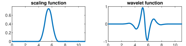
Figure 2: Scaling function and wavelet function.

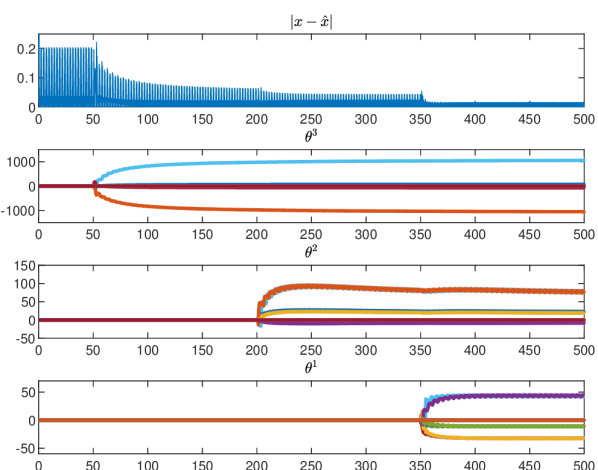
Figure 3: Time evolution of the state-estimation error $x-\hat{x}$ and of the identifier’s parameters $\theta^{i}$ in the first case in which $\phi=\phi_{1}$.

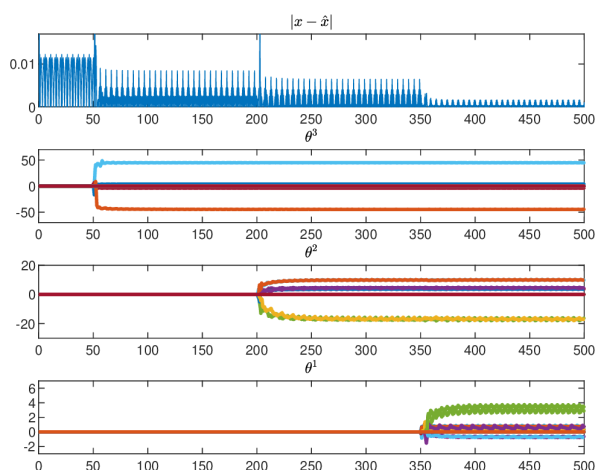
Figure 4: Time evolution of the state-estimation error $x-\hat{x}$ and of the identifier’s parameters $\theta^{i}$ in the second case in which $\phi=\phi_{2}$.

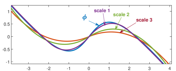
Figure 5: Approximation of $\phi=\phi_{2}$ at the different scales.

The knowledge of $\mathcal{X}$ and $\mathcal{X}_{0}$, defined above, allows us to construct an adaptive observer as specified in Section II and Theorem 1, by taking $X^{\star}$ so that $\mathcal{X}\subset\mathrm{X}^{\star}$ and $\Xi^{\star}$ large enough to handle all the functions $\phi$ of interest (for instance $\Xi^{\star}:=\{x\in\mathbb{R}^{2}\,\mid\,|x|\leq 10^{3}\}$ allows to handle both (33)). For the identification phase, we use the multiresolution identifier of Section IV-B to perform a wavelet expansion of $\phi$. Since $\phi$ depends only on $x_{1}$, for ease of exposition we limit to 1-dimensional wavelets, i.e. in Section IV-B we consider functions $\hat{\phi}(\theta,\cdot)$ inside $L^{2}(\mathbb{R})$ depending only on $x_{1}$. We choose a biorthogonal B-spline construction for the scaling and wavelet functions, both represented in Figure 2, and we fix $i_{0}:=3$ as the starting scale and $i_{T}:=1$ as the target one, requiring thus the use of $N=3$ least-squares stages.

In the presented simulations, the three stages are added progressively at successive instants of time. For the first $50$ seconds no identifier is present, and a canonical high-gain observer obtained with $\psi=0$ is thus used. At time $50s$, a first stage $z^{3}$ is added, working at the initial scale $i_{0}:=3$, and the function $\psi$ is modified accordingly. At time $200$s, a second stage $z^{2}$ is added to obtain a representation at scale $i_{0}-1=2$. Finally, at time $350$s, a third stage is added to reach a representation at scale $i_{T}=1$. The identifier samples and updates every $T=0.1$ seconds. To ensure that Assumption 4 holds, we set the regularization matrices of each stage to $R^{i}=10^{-3}I_{n_{\theta}^{i}}$. The forgetting factors are chosen as $\mu^{3}:=0.999$, $\mu^{2}:=0.995$, and $\mu^{1}:=0.99$. The design of the observer is then concluded by taking $g=25$.

Two simulations have been obtained by applying the same observer to (32) with $x(0)=(-2.5,3)$ and with $\phi$ taken equal to $\phi_{1}$ and $\phi_{2}$ of (33) respectively. Figures 3 and 4 show the time evolution, in both cases, of the norm of the estimation error $x(t)-\hat{x}(t)$ and of the output $\theta^{i}(j)$ of each least-squares stage. Figure 5 shows instead the corresponding approximation of the function $\phi_{2}$ given by the models at the different scales associated with the final value of the estimated parameters.

V-B Least-Squares Estimation With Measurement Noise

According to the second claim of Theorem 1, and as typical of high-gain designs, measurement noise is the disturbance having the worst effect on the estimates, as it gets amplified by a worst-case factor of $g^{n}$. Nevertheless, according to the claim of Theorem 1, the measurement noise acts “continuously” on the asymptotic bound on the state and parameter estimates. Therefore we may expect such estimates to behave still reasonably well for small enough noise, where “small enough” depends on the fixed control parameter $g$.

By this example we aim to show how the measurement noise affects the performance of parameter and state estimation when the proposed adaptive observer is used together with the least-squares identifier of Section IV-A.

We consider the following class of systems

$$\begin{array}[]{lcl}\dot{x}_{1}&=&x_{2}\\ \dot{x}_{2}&=&x_{3}\\ \dot{x}_{3}&=&\alpha x_{2}+3\beta x_{1}^{2}x_{2}+\ell((1-x_{1}^{2})x_{3}-2x_{1}x_{2}^{2})\\ y&=&x_{1}+\nu\end{array}$$ (34)

in which $\theta_{\rm T}:=(\alpha,\beta,\ell)\in\mathbb{R}^{3}$ is an unknown parameter, and $\nu$ is a disturbance acting on the measured output $y$. For different initial conditions and values of $\theta_{\rm T}$, System (34) models different linear and nonlinear oscillators, as for instance the (extended) Duffing and Van der Pol oscillators [29].

We suppose that $\theta_{\rm T}$ ranges in a compact set $\Theta^{\star}\subset[-5,\,5]\times[-5,0]\times[0,\,5]$ whose elements are such that Assumption 1 holds with $\mathcal{X}_{0}=[-2,\,2]^{3}$ and $\mathcal{X}:=[-10,\,10]\times[-10,\,10]\times[-100,\,100]$. Based on this, in the following simulations we have chosen the observer degrees of freedom as follows:

1. In (4)-(5), we let $\underline{\rm T}=\overline{\rm T}=1/2$, and we chose $\Lambda_{1}$ and $\Lambda_{2}$ according to (13), with $K=(4,\,6,\,4,\,1)$.

2. We defined the identifier’s data $(\mathcal{M},\mathcal{Z},\varphi,\gamma)$ as specified in the least squares section (Section IV-A) with ${n_{\theta}}=3$, $\mu=0.995$, $R=0$, $\sigma=\operatorname{col}(\sigma_{1},\,\sigma_{2},\,\sigma_{3})$, with $\sigma_{1}(x):=x_{2}$, $\sigma_{2}(x)=3x_{1}^{2}x_{2}$, $\sigma_{3}(x):=(1-x_{1}^{2})x_{3}-2x_{1}x_{2}^{2}$, and with $(\varphi,\gamma)$ chosen according to (22) with

   $$\Sigma(\alpha_{\rm in}) :=\operatorname{sat}_{c_{\Sigma}}\big{(}\sigma(\alpha_{\rm in})\sigma(\alpha_{\rm in})^{\top}\big{)}$$

   $$\lambda(\alpha_{\rm in},\alpha_{\rm out}) :=\operatorname{sat}_{c_{\lambda}}\big{(}\sigma(\alpha_{\rm in})\alpha_{\rm out}\big{)}$$

   $$\gamma(z) :=\operatorname{sat}_{c_{\gamma}}\big{(}z_{1}^{\dagger}z_{2}\big{)},$$

   in which $\operatorname{sat}$ denotes the component-wise saturation function, and $c_{\Sigma}=10^{7}$, $c_{\lambda}=10^{8}$ and $c_{\gamma}=10$.

3. According to Section II-B, and to the least-squares choice $\hat{\phi}(\theta,\cdot)=\theta^{\top}\sigma(\cdot)$, $\psi$ is chosen as

   $$\psi(\theta,\hat{x},\xi) =\operatorname{sat}_{M}\left(\theta^{\top}\dfrac{\partial\sigma(\hat{x})}{\partial\hat{x}}\operatorname{col}(\hat{x}_{2},\hat{x}_{3},\xi)\right)$$

   $$=\operatorname{sat}_{M}\Big{(}\theta_{1}\hat{x}_{3}+\theta_{2}\big{(}6\hat{x}_{1}\hat{x}_{2}^{2}+3\hat{x}_{1}^{2}\hat{x}_{3}\big{)}$$

   $$\qquad\quad+\ell\big{(}(1-\hat{x}_{1}^{2})\xi-6\hat{x}_{1}\hat{x}_{2}\hat{x}_{3}-2\hat{x}_{2}^{3}\big{)}\Big{)},$$

   with $M=10^{3}$.

4. The design is concluded by choosing $g=25$.

Taking $R=0$ permits to have an asymptotic state and parameter estimate when the noise is not present. However, as remarked in Section IV-A, it implies that Claim 2 of Theorem 1 applies only to the solutions of (34) carrying enough excitation. While $c_{\gamma}$ is chosen on the basis of the knowledge of $\Theta^{\star}$, the saturation constants $M$, $c_{\Sigma}$ and $c_{\lambda}$ are chosen large enough so that, with $\phi(x):=\theta_{\rm T}^{\top}\sigma(x)$, we have $\psi(\theta_{\rm T},x,\phi(x))=(\partial\phi(x)/\partial x)\operatorname{col}(x_{2},x_{3},\phi(x))$, $\Sigma(x)=\sigma(x)\sigma(x)^{\top}$, and $\lambda(x,\phi(x))=\sigma(x)\phi(x)$ along the solutions to (34) of interest.

The following simulations have been obtained with $x(0)=(1,-1,0)$, $\tau(0)=0$, $\hat{x}(0)=(0,0,0)$, $\xi(0)=0$, $z_{1}(0)=I$, and $z_{2}(0)=0$. The unknown parameter $\theta_{\rm T}$ is initially set to

$$\theta_{\rm T}=(\alpha_{1},\beta_{1},\ell_{1})=(-1,0,1/2),$$

and later, around time $t=1000$, changed to

$$\theta_{\rm T}=(\alpha_{2},\beta_{2},\ell_{2})=(1,-1/2,0).$$

In a first simulation, we compare, in a noise-free setting, the adaptive observer constructed above with a non-adaptive extended high-gain observer obtained with $\psi=0$. As shown in Figure 6, with the adaptive observer the norm of the state estimation error $\hat{x}-x$ decays exponentially to zero (with a time constant determined by the parameter convergence), and the parameter $\theta$ converges to $\theta_{\rm T}$. The non-adaptive observer instead shows a persistent estimation error.

In the next simulations we let $\nu$ be given by

$$\nu(t)=q\nu_{0}(t),$$

in which $q>0$, and $\nu_{0}$ is obtained as a linear interpolation (in time) of the samples of an uniformly distributed stochastic process sampled every $0.1$ seconds, and taking values in $[-1/2,1/2]$. Figure 7 shows the parameter estimates obtained with $q=10^{-3}$, $q=5\cdot 10^{-3}$ and $q=10^{-2}$ respectively. Clearly, as the noise amplitude increases, the parameter estimation performance decreases. Nevertheless, the continuity between noise amplitude and asymptotic estimation error claimed in Theorem 1 is evident from the plots.

Finally, Figure 8 shows the time evolution of the norm $|\hat{x}-x|$ of the state estimation error for the different noise levels. In presence of sufficiently small measurement noise, the proposed adaptive observer still performs considerably better than the non-adaptive one. However, as the noise amplitude increases, its effect on the state estimate becomes more important, dominating the effect of adaptation. Thus, as the noise amplitude increases, the performance of the adaptive observer gets close to the non-adaptive case, as evident in Figure 8.

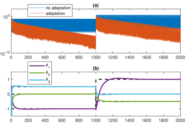
Figure 6: Comparison, in a noise-free setting, between the proposed adaptive observer and a non-adaptive extended high-gain observer obtained with $\psi=0$. Plot (a) shows, in semi-logarithmic scale, the time evolution of the norm $|\hat{x}-x|$ of the state estimation error. Plot (b) shows the time-evolution of the parameter estimate $\theta$ obtained by the adaptive observer. The values of $\theta_{\rm T}$ is depicted in dashed, gray line.

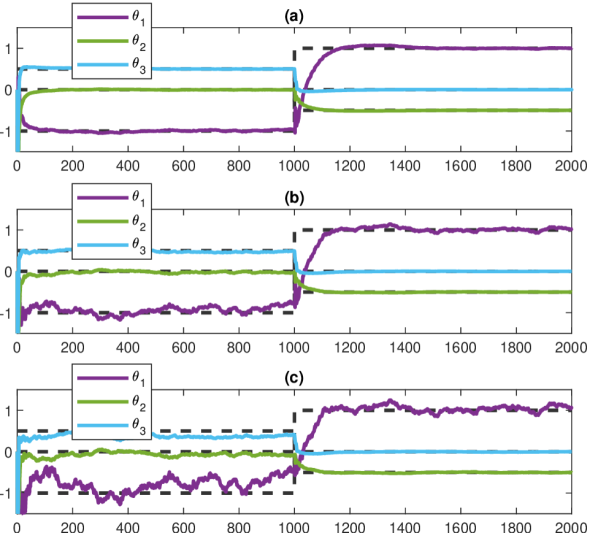
Figure 7: Time evolution of the parameter estimate with different noise levels. Plot (a) is obtained with $q=10^{-3}$, plot (b) with $q=5\cdot 10^{-3}$, and (c) with $q=10^{-2}$.

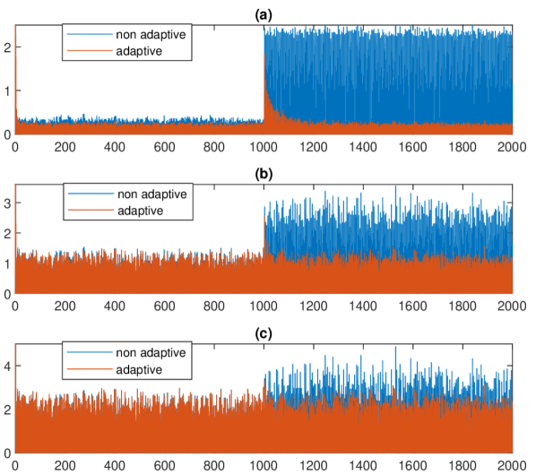
Figure 8: Time evolution of the state estimate $|\hat{x}-x|$ with different noise levels. Plot (a) is obtained with $q=10^{-3}$, plot (b) with $q=5\cdot 10^{-3}$, and (c) with $q=10^{-2}$.

VI Conclusions

In this paper we considered the problem of joint state and model estimation for a class of nonlinear systems. We proposed an adaptive observer in which adaptation is cast and solved as a system identification problem. Practical and approximate estimation results are given, and robustness with respect to exogenous disturbances is provided in terms of an input-to-state stability property. Differently from canonical adaptive observer designs, here we did not assume a particular structure of the uncertainty and we did not propose an ad hoc adaptation mechanism. Rather, different parametric and non-parametric system identification techniques can be applied. Future research will focus on the extension of the framework to more general classes of systems and observers and to the application to output-feedback stabilization and regulation.

-A Proof of Theorem 1

To prove the first claim, change coordinates as

$$\hat{x}_{i}\mapsto\tilde{x}_{i}:=g^{1-i}(\hat{x}_{i}-x_{i})$$

and define $\zeta:=\operatorname{col}(\tilde{x},g^{-n}\xi)$. Then $\zeta$ flows according to

$$\dot{\zeta}=gM\zeta+H_{1}(g)\psi(\theta,\hat{x},\xi)-H_{2}(g)d-H_{3}(g)\phi(x)+g\Lambda(1)\nu,$$

in which $\Lambda:=\operatorname{col}(\Lambda_{1},\Lambda_{2})$, $H_{1}(g):=g^{-n}\operatorname{col}(0_{p},B)$, $H_{2}(g):=\operatorname{col}\big{(}\operatorname{diag}(I_{p},g^{-1}I_{p},\dots,g^{1-n}I_{p}),\,0_{{p}\times{n{p}}}\big{)}$, and $H_{3}(g):=g^{1-n}\operatorname{col}(B,0_{p})$, and $M$ is defined in (12). Moreover, $\zeta$ jumps as $\zeta^{+}=\zeta$. Hence, in view of (15), and since by Assumption 1 $\phi(\mathcal{X})$ is bounded and $x(t)\in\mathcal{X}$ whenever $x(0)\in\mathcal{X}_{0}$ and $d\in\mathbb{D}(x(0))$, standard high-gain arguments (see e.g. [22]) show that for some $a_{0},a_{1},a_{2}>0$, and with ${\rm d}_{g}$ defined in (17),

$$|\zeta(t,j)|\leq\max\Big{\{}a_{0}{\rm e}^{-a_{1}gt}|\zeta(0)|,\,g^{-n}a_{0},\,a_{0}|({\rm d}_{g},\nu)|_{t}\Big{\}}$$

holds for each $(t,j)\in\operatorname{dom}\zeta$, from which the first claim of the theorem can be easily deduced.

Regarding the second claim, first notice that, by definition of $\mathrm{C}_{\tau}$ and $\mathrm{D}_{\tau}$ in (5), every complete solution $\mathbf{x}$ of (16) has infinite jumps and flows, i.e. $\sup\operatorname{Jmp}\mathbf{x}=\sup\operatorname{Flw}\mathbf{x}=\infty$. Pick a complete solution pair $(\mathbf{x},(d,\nu))$ to (16) and let $z^{\star}$ and $\theta^{\star}$ be the corresponding hybrid arcs produced by the Identifier Requirement. Change variables as

$$\xi\mapsto\tilde{\xi}:=g^{-n}(\xi-\hat{\phi}(\theta^{\star},x)),$$

and let $\tilde{\zeta}:=\operatorname{col}(\tilde{x},\tilde{\xi})$. Then, noting that $\xi-\phi(x)=g^{n}\tilde{\xi}-\varepsilon^{\star}$, it is readily seen that $\tilde{\zeta}$ flows according to

$$\dot{\tilde{\zeta}}=gM\tilde{\zeta}+H_{1}(g)\tilde{\psi}(\theta,\theta^{\star},\tilde{x},\tilde{\xi},x)-H_{2}(g)d-H_{3}(g)\varepsilon^{\star}+g\Lambda(1)\nu,$$

in which, by letting $G(g):=\operatorname{diag}(I_{p},gI_{p},\dots,g^{n-1}I_{p})$,

$$\tilde{\psi}(\theta,\theta^{\star},\tilde{x},\tilde{\xi},x) :=\psi\big{(}\theta,x+G(g)\tilde{x},g^{n}\tilde{\xi}+\hat{\phi}(\theta^{\star},x)\big{)}$$

$$\qquad-\dfrac{\partial\hat{\phi}(\theta^{\star},x)}{\partial x}\big{(}Ax+B\phi(x)+d\big{)}.$$

Furthermore, $\tilde{\zeta}$ jumps according to

$$\tilde{\zeta}^{+}=\tilde{\zeta}+H_{1}(g)\big{(}\varepsilon^{\star}{}^{+}-\varepsilon^{\star}\big{)}.$$

By the Identifier Requirement, there exists $j^{\star}\in\mathbb{N}$ such that $z^{\star}(j)\in\mathrm{Z}^{\star}$ (and hence $\theta^{\star}(j)\in\gamma(\mathrm{Z}^{\star})\subset\Theta^{\star}$) for all $j\geq j^{\star}$. Thus, if $(x,\phi(x))$ is eventually in $X^{\star}\times\Xi^{\star}$, there exists $\bar{s}\in\operatorname{dom}\mathbf{x}$ of the form $\bar{s}=(t_{\bar{j}},\bar{j})$ with $\bar{j}\in\operatorname{Jmp}\mathbf{x}$ satisfying $\bar{j}\geq j^{\star}$, such that $(x(t,j),\phi(x(t,j)),\theta^{\star}(t,j))\in X^{\star}\times\Xi^{\star}\times\Theta^{\star}$ for all $(t,j)\succeq\bar{s}$. Hence, in view of (14) and of the regularity item of the Identifier Requirement there exist $a_{4},a_{5}>0$ such that

$$|\tilde{\psi}(\theta,\theta^{\star},\tilde{x},\tilde{\xi},x)|\leq a_{4}\big{(}g^{n}|\tilde{\zeta}|+|z-z^{\star}|+|\varepsilon^{\star}|+|d|\big{)}$$

for all $(t,j)\succeq\bar{s}$. We thus conclude that there exist $b_{0},b_{1},b_{2}>0$ and $g^{\star}_{a}>0$ such that, if $g\geq g^{\star}_{a}$, $\tilde{\zeta}$ satisfies

$$|\tilde{\zeta}(t,j)| \leq b_{0}\max\Big{\{}{\rm e}^{-b_{1}g(t-t_{j})}|\tilde{\zeta}(t_{j},j)|,\,g^{-n}|\varepsilon^{\star}|_{(t,j)},$$ (35)

$$\qquad\qquad\qquad g^{-(n+1)}|z-z^{\star}|_{j},\,|({\rm d}_{g},\nu)|_{t}\Big{\}}$$

$$|\tilde{\zeta}(t,j+1)| \leq 2\max\big{\{}|\tilde{\zeta}(t,j)|,\,2g^{-n}|(\varepsilon^{\star}(t,j),\varepsilon^{\star}{}(t,j+1))|\big{\}}$$

respectively during the flow and jump times succeeding $\bar{s}$, and with $\tilde{\zeta}(\bar{s})$ that is bounded according to the first claim of the theorem. We then observe that, since for each $j\in\operatorname{Jmp}\mathbf{x}$ it holds that $t^{j}-t_{j}\geq\underline{\rm T}$, then for each constant $\bar{b}>0$, taking $g$ sufficiently large yields

$$\lim_{t+j\to\infty}\bar{b}^{j+1}{\rm e}^{-b_{1}gt}\leq\lim_{j\to\infty}=\bar{b}^{j+1}{\rm e}^{-jb_{1}g\underline{\rm T}}=0.$$

Therefore, there follows from (35) by induction and standard ISS arguments (see e.g. [30]) that there exist $c_{1},c_{2}>0$ and $g^{\star}_{b}(\underline{\rm T})>g_{a}^{\star}$ such that $g\geq g_{b}^{\star}(\underline{\rm T})$ implies

$$\limsup_{t+j\to\infty}|\tilde{\zeta}|\leq\max\Big{\{} c_{1}g^{-n}\limsup_{t+j\to\infty}|\varepsilon^{\star}|,\,c_{2}\limsup_{t\to\infty}|({\rm d}_{g},\nu)|$$ (36)

$$\ c_{2}g^{-(n+1)}\limsup_{j\to\infty}|z-z^{\star}|\Big{\}},$$

where we used the fact that $\limsup_{t+j\to\infty}|\varepsilon^{\star}|=\limsup_{t+j\to\infty}|\varepsilon^{\star}{}^{+}|$. On the other hand, the identifier is subject to the inputs $(\alpha_{\rm in},\alpha_{\rm out})=(\alpha_{\rm in}^{\star}+\delta_{\rm in},\alpha_{\rm out}^{\star}+\delta_{\rm out})$ with $(\alpha_{\rm in}^{\star},\alpha_{\rm out}^{\star})=(x,\phi(x))$ and

$$\delta_{\rm in} =G(g)\tilde{x}, \delta_{\rm out} =g^{n}\tilde{\xi}-\varepsilon^{\star},$$

in which we recall that $G(g):=\operatorname{diag}(I_{p},gI_{p},\dots,g^{n-1}I_{p})$. Therefore, the stability item of the Identifier Requirement yields the estimate

$$\limsup_{j\to\infty}|z-z^{\star}|\leq c_{3}\max\Big{\{}g^{n}\limsup_{t+j\to\infty}|\tilde{\zeta}|,\,\limsup_{t+j\to\infty}|\varepsilon^{\star}|\Big{\}}$$ (37)

with $c_{3}>0$ proportional to the Lipschitz constant of $\rho_{z}$. Pick

$$g>g^{\star}(\underline{\rm T}):=\max\big{\{}g_{b}^{\star}(\underline{\rm T}),\,c_{1},\,c_{3}c_{2}\big{\}},$$

then substituting (37) into (36), and assuming without loss of generality $c_{1}\geq 1$, shows that

$$\limsup_{t+j\to\infty}|\tilde{\zeta}|\leq\max\Big{\{}g^{1-n}\limsup_{t+j\to\infty}|\varepsilon^{\star}|,\,c_{2}\limsup_{t\to\infty}|({\rm d}_{g},\nu)|\Big{\}},$$ (38)

and substituting (36) into (37) yields

$$\limsup_{j\to\infty}|z-z^{\star}|\leq\max\Big{\{}\!c_{4}\limsup_{t+j\to\infty}|\varepsilon^{\star}|,c_{5}g^{n}\limsup_{t\to\infty}|({\rm d}_{g},\nu)|\!\Big{\}}$$ (39)

with $c_{4}:=c_{1}c_{3}$ and $c_{5}:=c_{2}c_{3}$. Thus, the first equation of the second claim follows directly by (38) and (39) in view of the regularity item of the Identifier Requirement. The second equation instead follows by (38) once noted that $|\hat{x}_{i}-x_{i}|\leq g^{i-1}|\tilde{\zeta}|$.

-B Proof of Proposition 1

By definition of $\Sigma$ and $\lambda$ in (20), they are bounded and Lipschitz on $X^{\star}$ and $X^{\star}\times\Xi^{\star}$ respectively. Hence, there exists $\ell>0$ such that, for each $x_{1}\in X^{\star}$, $x_{2}\in\mathbb{R}^{n}$, $y_{1}\in\Xi^{\star}$ and $y_{2}\in\mathbb{R}$ it holds that

$$|\Sigma(x_{1})-\Sigma(x_{2})| \leq\ell|x_{1}-x_{2}|,$$ (40)

$$|\lambda(x_{1},y_{1})-\lambda(x_{2},y_{2})| \leq\ell|(x_{1},y_{1})-(x_{2},y_{2})|.$$

Pick a solution pair $((\tau,x),d)$ to (6) with $x(0)\in\mathcal{X}_{0}$ and $d\in\mathbb{D}(x(0))$. Define $z^{\star}=(z_{1}^{\star},z_{2}^{\star})$ by letting $z^{\star}(0)=(0,0)$ and, for $j\geq 1$,

$$z_{1}^{\star}(j) :=\sum_{i=0}^{j-1}\mu^{j-i-1}\sigma(x(t^{i}))\sigma(x(t^{i}))^{\top}$$

$$z_{2}^{\star}(j) :=\sum_{i=0}^{j-1}\mu^{j-i-1}\sigma(x(t^{i}))\phi(x(t^{i})).$$

Since by Assumption 3 $(x(t),\phi(x(t)))\in X^{\star}\times\Xi^{\star}$ then, for $\delta=0$, $((\tau,x,z^{\star}),(d,\delta))$ is a solution pair to (10).

By construction, $|z_{1}^{\star}(j)|\leq c_{1}$ and $|z_{2}^{\star}(j)|\leq c_{2}$, with $c_{1}$ and $c_{2}$ defined in (19). By Assumption 2, for $j\geq j^{\star}$, $\operatorname{msv}(z_{1}^{\star}(j)+R)\geq\epsilon$, so that $z^{\star}(j)\in\mathrm{Z}^{\star}$ for all $j\geq j^{\star}$.

Next, let $\mathcal{J}_{(\tau,x)}$ given by (18). Then, for all $j\in\mathbb{N}$

$$\operatorname{Opt}_{(\tau,x)}(j) =\left\{\theta\in\mathbb{R}^{n_{\theta}}\,\mid\,\dfrac{\partial\mathcal{J}_{(\tau,x)}(j,\theta)}{\partial\theta}=0\right\}$$

$$=\Big{\{}\theta\in\mathbb{R}^{n_{\theta}}\,\mid\,(z_{1}^{\star}(j)+R)\theta=z_{2}^{\star}(j)\Big{\}}.$$

As $z_{2}^{\star}(j)\in\operatorname{Im}z_{1}^{\star}(j)$, and since $z^{\star}(j)\in\mathrm{Z}^{\star}$ implies $\gamma(z^{\star}(j))=(z_{1}^{\star}(j)+R)^{\dagger}z_{2}^{\star}(j)$, then $\theta^{\star}:=\gamma(z^{\star})$ satisfies $\theta^{\star}(j)\in\operatorname{Opt}_{(\tau,x)}(j)$ for all $j\geq j^{\star}$. Thus, the optimality requirement holds.

Moreover, pick a solution pair to (10) of the form $((\tau,x,z),(d,\delta))$, with $((\tau,x),d)$ the same as above. By direct solution we also obtain

$$|z(j)-z^{\star}(j)|\leq\mu^{j}|z(0)-z^{\star}(0)|$$

$$+\sum_{i=0}^{j-1}\mu^{j-i-1}\big{(}|\Sigma(x(t^{i}))-\Sigma(x(t^{i})+\delta_{\rm in}(t^{i}))|$$

$$+|\lambda(x(t^{i}),\phi(x(t^{i})))-\lambda(x(t^{i})+\delta_{\rm in}(t^{i}),\phi(x(t^{i}))+\delta_{\rm out}(t^{i}))|\big{)}$$

which in view of (40) yields

$$|z(j)-z^{\star}(j)|\leq 2\max\Big{\{}\mu^{j}|z(0)-z^{\star}(0)|,2\ell(1-\mu)^{-1}|\delta|_{j}\Big{\}}$$

which is the stability requirement.

Finally, since $\gamma$ is Lipschitz on $\mathrm{Z}^{\star}$ and bounded, there exists $\rho_{\theta}>0$ such that, for all $(z,z^{\star})\in\mathcal{Z}\times\mathrm{Z}^{\star}$, $|\gamma(z)-\gamma(z^{\star})|\leq\rho_{\theta}|z-z^{\star}|$, which implies the first part of the regularity item. The second part, instead, holds by definition of $\sigma$.

-C Basics of Wavelet Analysis

For the basic concepts about wavelets, Riesz bases and biorthogonality, we refer to [31, 32, 33, 34]. A relevant framework in which biorthogonal wavelets can be constructed is the Generalized Multiresolution Analysis (GMRA) [32].

Definition 2.

A GMRA on $\mathbb{R}$ is a sequence of subspaces $(V_{i})_{i\in\mathbb{Z}}$ of $L^{2}(\mathbb{R})$ satisfying the following properties:

1. For all $i\in\mathbb{Z}$, $V_{i}\subset V_{i-1}$.

2. For any $f\in\mathbb{C}_{c}(\mathbb{R})$ and every $\epsilon>0$, there exist $i\in\mathbb{Z}$ and a function $g\in V_{i}$ such that $|f-g|\leq\epsilon$.

3. $\cap_{i\in\mathbb{Z}}V_{i}=\{0\}$.

4. $f\in V_{i}$ if and only if $f(2^{i}\cdot)\in V_{0}$.

5. There exists a function $\varphi\in L^{2}(\mathbb{R})$, called the scaling function, such that $V_{0}=\overline{\operatorname{span}}\{\varphi(\cdot-k)\}_{k\in\mathbb{Z}}$ and $\{\varphi(\cdot-k)\}_{k\in\mathbb{Z}}$ is a Riesz basis for $V_{0}$.

For a function $f\in L^{2}(\mathbb{R})$ and with $i,k\in\mathbb{Z}$, we define the function $f_{i,k}\in L^{2}(\mathbb{R})$ as $f_{i,k}(s)=2^{-i/2}f(2^{-i}s-k)$. If $\varphi$ is a scaling function of a GMRA $(V_{i})_{i\in\mathbb{Z}}$, then $V_{i}=\overline{\operatorname{span}}\{\varphi_{i,k}\}_{k\in\mathbb{Z}}$ and $\{\varphi_{i,k}\}_{k\in\mathbb{Z}}$ is a Riesz basis for $V_{i}$. As the family $\{\varphi(\cdot-k)\}_{k\in\mathbb{Z}}$ is a Riesz basis of $V_{0}$, it admits a dual basis $\{\widetilde{\varphi}(\cdot-k)\}_{k\in\mathbb{Z}}$. If $\widetilde{\varphi}$ is the scaling function of a GMRA $(\widetilde{V}_{i})_{i\in\mathbb{Z}}$ we say that the GMRAs $(V_{i})_{i\in\mathbb{Z}}$ and $(\widetilde{V}_{i})_{i\in\mathbb{Z}}$ are dual to each other. With $i\in\mathbb{Z}$ and $f\in L^{2}(\mathbb{R})$ we define the projection operator ${\rm P}_{i}$ and the detail operator ${\rm Q}_{i}$ as

$${\rm P}_{i}f:=\sum_{k\in\mathbb{Z}}\langle f,\widetilde{\varphi}_{i,k}\rangle\varphi_{i,k},\qquad{\rm Q}_{i}f:={\rm P}_{i-1}f-{\rm P}_{i}f.$$

For a given $i\in\mathbb{Z}$, ${\rm Q}_{i}f$ represents the additional detail that is needed to obtain a finer approximation ${\rm P}_{i-1}f$ of $f$ at scale $i-1$ starting from a coarser approximation ${\rm P}_{i}f$ at scale $i$. Moreover, for every $f\in\mathbb{C}_{c}(\mathbb{R})$, $\lim_{i\to-\infty}|{\rm P}_{i}f-f|=0$.

We can univocally associate with the scaling functions $\varphi$ and $\widetilde{\varphi}$, respectively, two functions $\psi$ and $\widetilde{\psi}$ in $L^{2}(\mathbb{R})$, called the wavelet functions. With $W_{i}:=\overline{\operatorname{span}}\{\psi_{i,k}\}_{k\in\mathbb{Z}}$ and $\widetilde{W}_{i}:=\overline{\operatorname{span}}\{\psi_{i,k}\}_{k\in\mathbb{Z}}$, they fulfill the following properties.

1. $\psi\in V_{-1}$ and $\widetilde{\psi}\in\widetilde{V}_{-1}$.

2. $\{\psi_{0,k}\}_{k\in\mathbb{Z}}$ and $\{\widetilde{\psi}_{0,k}\}_{k\in\mathbb{Z}}$ are biorthogonal.

3. $\{\psi_{0,k}\}_{k\in\mathbb{Z}}$ is a Riesz basis for $W_{0}$ and $\{\widetilde{\psi}_{0,k}\}_{k\in\mathbb{Z}}$ is a Riesz basis for $\widetilde{W}_{0}$.

4. For all $k,\ell\in\mathbb{Z}$, $\langle\psi_{0,k},\widetilde{\varphi}_{0,\ell}\rangle=0$ and $\langle\widetilde{\psi}_{0,k},\varphi_{0,\ell}\rangle=0$.

5. For all $f\in\mathbb{C}_{c}(\mathbb{R})$, ${\rm Q}_{0}f\in W_{0}$.

Directly from the definition of ${\rm P}_{i}$ and ${\rm Q}_{i}$ we obtain that, for all $i,i_{0}\in\mathbb{Z}$ such that $i\leq i_{0}$, the following holds

$${\rm P}_{i}f=\sum_{k\in\mathbb{Z}}a_{i_{0},k}\varphi_{i_{0},k}+\sum_{\ell=i+1}^{i_{0}}\sum_{k\in\mathbb{Z}}b_{\ell,k}\psi_{\ell,k}$$ (41)

with $a_{i_{0},k}:=\langle f,\widetilde{\varphi}_{i_{0},k}\rangle$ and $b_{\ell,k}:=\langle f,\widetilde{\psi}_{\ell,k}\rangle$.

Wavelet theory can be extended to deal with multivariable functions in $L^{2}(\mathbb{R}^{m})$, $m>1$, by considering the tensor product of $m$ GMRAs (see [31]). More precisely, for each $i\in\mathbb{Z}$, we define the subspace $\mathbf{V}_{i}$ as $\mathbf{V}_{i}:=V_{i}\otimes V_{i}\otimes\cdots\otimes V_{i}=\overline{\operatorname{span}}\{\Phi_{i,\mathbf{k}}(x),\,\mathbf{k}\in\mathbb{Z}^{m}\}$, in which, with $\mathbf{k}=(k_{1},\dots,k_{m})\in\mathbb{Z}^{m}$, $\Phi_{i,\mathbf{k}}(x):=\varphi_{i,k_{1}}(x_{1})\cdots\varphi_{i,k_{m}}(x_{m})$. Then $(\mathbf{V}_{i})_{i\in\mathbb{Z}}$ forms a GMRA on $L^{2}(\mathbb{R}^{m})$ (i.e. satisfying analogous properties of Definition 2) such that $f\in\mathbf{V}_{i}\iff f(2^{i}\cdot)\in\mathbf{V}_{0}$, and in which $\Phi:=\Phi_{0,0}$ plays the role of a scaling function and the functions $\Phi_{i,\mathbf{k}}(x)$, $\mathbf{k}\in\mathbb{Z}^{m}$, form a Riesz basis for $\mathbf{V}_{i}$. In the same way we construct the dual GMRA $(\widetilde{\mathbf{V}}_{i})_{i\in\mathbb{Z}}$ and its scaling function $\widetilde{\Phi}$. For every $i\in\mathbb{Z}$ and $\mathbf{k}\in\mathbb{Z}^{m}$, we construct $2^{m}-1$ wavelet functions $\Psi^{h}_{i,\mathbf{k}}$, $h=1,\dots,2^{m}-1$, by taking all the possible combinations of products of the form $g_{1}(x_{1})g_{2}(x_{2})\cdots g_{m}(x_{m})$, with $g_{\ell}(x_{\ell})$ taking the value $\varphi_{i,k_{\ell}}(x_{\ell})$ or $\psi_{i,k_{\ell}}(x_{\ell})$, except for the case in which $g_{\ell}(x_{\ell})=\varphi_{i,k_{\ell}}(x_{\ell})$ for all $\ell=1,\dots,m$. Namely,

$$\Psi_{i,\mathbf{k}}^{1}(x) :=\psi_{i,k_{1}}(x_{1})\varphi_{i,k_{2}}(x_{2})\cdots\varphi_{i,k_{m}}(x_{m})$$

$$\Psi_{i,\mathbf{k}}^{2}(x) :=\varphi_{i,k_{1}}(x_{1})\psi_{i,k_{2}}(x_{2})\varphi_{i,k_{3}}(x_{3})\cdots\varphi_{i,k_{m}}(x_{m})$$

$$\cdots$$

$$\Psi_{i,\mathbf{k}}^{2^{m}-1}(x) :=\psi_{i,k_{1}}(x_{1})\psi_{i,k_{2}}(x_{2})\psi_{i,k_{3}}(x_{3})\cdots\psi_{i,k_{m}}(x_{m}).$$

It can be shown that for every $i,i_{0}\in\mathbb{Z}$ such that $i\leq i_{0}$, we can express the projection of a function $f\in\mathcal{C}_{c}(\mathbb{R}^{m})$ into $\mathbf{V}_{i}$ by the following expansion generalizing (41)

$${\rm P}_{i}f=\sum_{\mathbf{k}\in\mathbb{Z}^{m}}a_{i_{0},\mathbf{k}}\Phi_{i_{0},\mathbf{k}}+\sum_{h=1}^{2^{m}-1}\sum_{\ell=i+1}^{i_{0}}\sum_{\mathbf{k}\in\mathbb{Z}^{m}}b_{\ell,\mathbf{k}}^{h}\Psi_{\ell,\mathbf{k}}^{h}.$$ (42)

In the general case, in the wavelet expansion (42) the sum in $\mathbf{k}$ ranges over the whole set $\mathbb{Z}^{m}$. Hence, even for fixed scale $i$, (42) might consist of infinite terms. Nevertheless, if compactly supported biorthogonal wavelet and scaling functions are used, the expansion (42) reduces to a finite sum for each $i$ whenever $f$ has bounded support.

Some famous families of wavelets with compact support are for instance the Daubechies wavelets [31] or the B-spline biorthogonal wavelets of [35]. They mix compact support, smoothness and symmetry.

References

- [1] R. Marino, G. L. Santosuosso, and P. Tomei, “Robust adaptive observers for nonlinear systems with bounded disturbances,” IEEE Trans. Autom. Control, vol. 46, no. 6, pp. 967–972, 2001.
- [2] L. Grüne and J. Pannek, Nonlinear Model Predictive Control. Springer, 2017.
- [3] M. Krstic, Delay Compensation for Nonlinear, Adaptive, and PDE Systems. Birkhäuser, 2009.
- [4] A. Isidori, Lectures in Feedback Design for Multivariable Systems. Springer International Publishing, 2017.
- [5] S. M. Kay, Fundamentals of Statistical Processing, Volume I: Estimation Theory. Prentice Hall, 1993.
- [6] A. Cichocki and S. Amari, Adaptive Blind Signal and Image Processing: Learning Algorithms and Applications. John Wiley & Sons, Ltd, 2002.
- [7] G. Bastin and M. Gevers, “Stable adaptive observers for nonlinear time varying systems,” IEEE Trans. Autom. Control, vol. 33, no. 7, pp. 650–658, 1988.
- [8] R. Marino and P. Tomei, “Global adaptive observers for nonlinear systems via filtered transformations,” IEEE Trans. Autom. Control, vol. 37, no. 8, pp. 1239–1245, 1992.
- [9] ——, “Adaptive observers with arbitrary exponential rate of convergence for nonlinear systems,” IEEE Trans. Autom. Control, vol. 40, no. 7, pp. 1300–1304, 1995.
- [10] G. Besançon, “remarks on nonlinear adaptive observer design,” System & Control Letters, vol. 41, pp. 271–280, 2000.
- [11] Q. Zhang, “Adaptive observer for multiple-input-multiple-output (MIMO) linear time-varying systems,” IEEE Trans. Autom. Control, vol. 47, no. 3, pp. 525–529, 2002.
- [12] M. Farza, M. M’Saad, T. Maatoug, and M. Kamoun, “Adaptive observers for nonlinearly parametrized class of nonlinear systems,” Automatica, vol. 45, pp. 2292–2299, 2009.
- [13] I. Y. Tyukin, E. Steur, H. Nijmeijer, and C. van Leeuwen, “Adaptive observers and parameter estimation for a class of systems nonlinear in the parameters,” Automatica, vol. 49, pp. 2409–2423, 2013.
- [14] C. Afri, V. Andrieu, L. Bako, and P. Dufour, “State and parameter estimation: A nonlinear luenberger observer approach,” IEEE Trans. Autom. Control, vol. 62, no. 2, pp. 973–980, 2017.
- [15] G. Besançon and A. Ţiclea, “On adaptive observers for systems with state and parameter nonlinearities,” in Proc. 20th IFAC World Congress, Toulouse, France, 2017.
- [16] V. Andrieu and L. Praly, “On the existence of a Kazantzis-Kravaris/Luenberger observer,” SIAM J. Control Optim., vol. 45, no. 2, pp. 432–456, 2006.
- [17] G. Besançon and A. Ţiclea, “An immersion-based observer design for rank-observable nonlinear systems,” IEEE Trans. Autom. Control, vol. 52, no. 1, pp. 83–88, 2007.
- [18] D. Astolfi, M. Bin, L. Marconi, and L. Praly, “About robustness of internal model-based control for linear and nonlinear systems,” in accepted to the 58th IEEE Conference on Decision and Control (CDC), Miami Beach, FL, USA, 2018.
- [19] L. Ljung, System Identification: Theory for the user. Prentice Hall, 1999.
- [20] J. Sjöberg, Q. Zhang, L. Ljung, A. Benveniste, B. Delyon, P.-Y. Glorennec, H. Hjalmarsson, and A. Juditsky, “Nonlinear black-box modeling in system identification: a unified overview,” Automatica, vol. 31, no. 12, pp. 1691–1724, 1995.
- [21] A. Juditsky, H. Hjalmarsson, A. Benveniste, B. Delyon, L. Ljung, J. Söberg, and Q. Zhang, “Nonlinear black-box models in system identification: Mathematical foundations,” Automatica, vol. 31, no. 12, pp. 1725–1750, 1995.
- [22] H. K. Khalil, Nonlinear Systems. Third Edition. Upper Saddle River, New Jersey 07458: Prentice Hall, 2002.
- [23] A. Levant, “Robust exact differentiation via sliding mode technique,” Automatica, vol. 34, pp. 379–384, 1998.
- [24] V. Andrieu, L. Praly, and A. Astolfi, “Homogeneous approximation, recursive observer design, and output feedback,” SIAM J. Control Optim., vol. 47, no. 4, pp. 1814–1850, 2008.
- [25] R. Goebel, R. G. Sanfelice, and A. R. Teel, Hybrid Dynamical Systems. Princeton, N. J.: Princeton University Press, 2012.
- [26] J. Sjöberg, T. McKelvey, and L. Ljung, “On the use of regularization in system identification,” in IFAC 12th World Congress, 1993.
- [27] T. Söderström, “Errors-in-variables methods in system identification,” Automatica, vol. 43, pp. 939–958, 2007.
- [28] M. Milanese and C. Novara, “Set membership identification of nonlinear systems,” Automatica, vol. 40, pp. 957–975, 2004.
- [29] F. Forte, A. Isidori, and L. Marconi, “Robust design of internal models by nonlinear regression,” in Proc. 9th IFAC Symposium on Nonlinear Control Systems, 2013, pp. 283–288.
- [30] A. Isidori, Nonlinear Control Systems II. London, Great Britain: Springer-Verlag, 1999.
- [31] I. Daubechies, Ten Lectures on Wavelets. SIAM, 1992.
- [32] D. Walnut, An Introduction to Wavelets. Birkhäuser, 2002.
- [33] G. Strang and T. Nguyen, Wavelets and Filter Banks. Wellesley-Cambridge Press, 1996.
- [34] O. Christensen, Frames and Bases. Birkhäuser, 2008.
- [35] A. Cohen, I. Daubechies, and J. Feauveau, “Biorthogonal bases of compactly supported wavelets,” Communications on Pure and Applied Mathematics, vol. 45, no. 5, pp. 485–560, 1992.