A low-rank Lie-Trotter splitting approach for nonlinear fractional complex Ginzburg-Landau equations

Abstract

Fractional Ginzburg-Landau equations as the generalization of the classical one have been used to describe various physical phenomena. In this paper, we propose a numerical integration method for solving space fractional Ginzburg-Landau equations based on a dynamical low-rank approximation. We first approximate the space fractional derivatives by using a fractional centered difference method. Then, the resulting matrix differential equation is split into a stiff linear part and a nonstiff (nonlinear) one. For solving these two subproblems, a dynamical low-rank approach is used. The convergence of our method is proved rigorously. Numerical examples are reported which show that the proposed method is robust and accurate.

1 Introduction

In physics, the classical complex Ginzburg-Landau model, originally derived by Newell and Whitehead [1, 2], describes the amplitude evolution of waves in dissipative systems of fluid mechanics close to instabilities. This model has remarkable success in describing numerous phenomena including Bénard convection [1, 3], plane Poiseuille flow [4] and superconductivity [5, 6].

Tarasov and Zaslavsky [7, 8] first proposed a fractional generalization of the Ginzburg-Landau equation for fractal media. Later, fractional Ginzburg-Landau equations (FGLEs) have been used to describe various physical phenomena, refer e.g., to [9, 10, 11]. Many properties about FGLEs such as well-posedness, long-time dynamics and asymptotic behavior were studied; see [12, 13, 14, 15] and references therein. However, it is usually not possible to obtain analytical solutions of FGLEs, due to the non-local property of fractional derivatives. Thus, the development of efficient and reliable numerical techniques for solving FGLEs attracts many researchers. Wang and Huang [16] proposed an implicit midpoint difference scheme for FGLEs. Hao and Sun [17] proposed a linearized high-order difference scheme for the one-dimensional complex FGLE. Li and Huang [18] developed an implicit difference scheme for solving the coupled nonlinear FGLEs. In [19], the authors used an exponential Runge-Kutta method to solve the two-dimensional (2D) FGLE. Other related work can be found in [20, 21, 22, 23, 24] and references therein.

To the best of our knowledge, there are few numerical methods for solving FGLEs by using a dynamical low-rank approximation has been considered. Thus, in this paper, we mainly study a dynamical low-rank approximation [25] for solving the following 2D complex FGLE:

$$\begin{cases}\partial_{t}u-(\nu+\mathrm{\mathbf{i}}\eta)(\partial_{x}^{\alpha}+\partial_{y}^{\beta})u+(\kappa+\mathrm{\mathbf{i}}\xi)|u|^{2}u-\gamma u=0,&(x,y,t)\in\Omega\times(0,T],\\ u(x,y,0)=u_{0}(x,y),&(x,y)\in\bar{\Omega}=\Omega\cup\partial\Omega,\\ u(x,y,t)=0,&(x,y)\in\partial\Omega,\end{cases}$$ (1.1)

where $\mathrm{\mathbf{i}}=\sqrt{-1}$, $\nu>0,~{}\kappa>0,~{}\eta,~{}\xi$ are real numbers, $1<\alpha,~{}\beta<2$, $\Omega=(x_{L},x_{R})\times(y_{L},y_{R})\subset\mathbb{R}^{2}$, $u_{0}(x,y)$ is a given complex function, $\partial\Omega$ is the boundary of $\Omega$, and $\gamma\in\mathbb{R}$ is the coefficient of the linear evolution term. $\partial_{x}^{\alpha}$ and $\partial_{y}^{\beta}$ denote the Riesz fractional derivatives [26] in the $x$ and $y$ directions, respectively. More precisely, they are defined as follows:

$$\begin{split}&\partial_{x}^{\alpha}u(x,y,t)=-\frac{1}{2\cos(\alpha\pi/2)\Gamma(2-\alpha)}\frac{\partial^{2}}{\partial x^{2}}\int_{-\infty}^{\infty}\left|x-\zeta\right|^{1-\alpha}u(\zeta,y,t)d\zeta,\\ &\partial_{y}^{\beta}u(x,y,t)=-\frac{1}{2\cos(\beta\pi/2)\Gamma(2-\beta)}\frac{\partial^{2}}{\partial y^{2}}\int_{-\infty}^{\infty}\left|y-\zeta\right|^{1-\beta}u(x,\zeta,t)d\zeta.\end{split}$$

Moreover, if $\nu=\kappa=\gamma=0$, Eq. (1.1) becomes a nonlinear fractional Schrödinger equation [27]. Some numerical methods for such equations can be found in [28, 29, 30, 31].

Dynamical low-rank approximation was first studied by Koch and Lubich in [25]. It is a differential equation-based approach and mainly follows the idea of the Dirac-Frenkel variational principle [32, 33]. The aim of this approach is to find low-rank approximations to time-dependent large data matrices or to solutions of large matrix differential equations. This dynamical low-rank approach yields a differential equation for the approximation matrix on the low-rank manifold. Nonnenmacher and Lubich [34] first used this approach in different numerical applications, such as the compression of series of images and a blow-up problem of a reaction-diffusion equation. Lubich and Oseledets [35] proposed and analyzed an inexpensive integrator (called projector-splitting integrator) to numerically solve the differential equation arising from the dynamical low-rank approximation. Later, Kieri et al. [36] provided a comprehensive error analysis for the integration method. Note that their error bounds depend on the Lipschitz constant of the right-hand side of the considered matrix differential equation. Later, Ostermann et al. [37] proposed a integration method that yields low-rank approximations for stiff matrix differential equations. The key idea of their method is to first split the equation into stiff and nonstiff parts, and then to follow the dynamical low-rank approach. Their error analysis shows that the approach is independent of the stiffness and robust with respect to possibly small singular values in the approximation matrix. More dynamical low-rank based discretizations of high-dimensional time-dependent problems can be found in [38, 39, 40, 41, 42, 43].

The rest of this paper is organized as follows. In Section 2, we propose our low-rank approximation for solving Eq. (1.1). The error analysis of our method is given in Section 3. Two numerical examples provided in Section 4 strongly support the theoretical results. Concluding remarks are given in Section 5.

2 A low-rank approximation of the 2D complex FGLE

In this section, our low-rank approximation for solving Eq. (1.1) is derived. Such an approximation is usually based on a matrix differential equation. Thus, Eq. (1.1) is first discretized in space by an appropriate difference method and the resulting equations are then reformulated as a matrix differential equation.

2.1 The matrix differential equation

For two given positive integers $N_{x}$ and $N_{y}$, let $h_{x}=\frac{x_{R}-x_{L}}{N_{x}}$ and $h_{y}=\frac{y_{R}-y_{L}}{N_{y}}$. Then, the space can be discretized by $\Omega_{h}=\left\{(x_{i},y_{j})\mid 0\leq i\leq N_{x},0\leq j\leq N_{y}\right\}$. Let $u_{ij}(t)$ be the numerical approximation of $u(x_{i},y_{j},t)$. For approximating $\partial_{x}^{\alpha}u$ and $\partial_{y}^{\beta}u$ in Eq. (1.1), we choose the second-order fractional centered difference method proposed in [44]. Then, we have

$$\partial_{x}^{\alpha}u(x_{i},y_{j},t)=-h_{x}^{-\alpha}\sum_{k=-N_{x}+i}^{i}g_{k}^{\alpha}u_{i-k,j}(t)+\mathcal{O}(h_{x}^{2})=\delta_{x}^{\alpha}u_{ij}(t)+\mathcal{O}(h_{x}^{2})$$ (2.1)

and

$$\partial_{y}^{\beta}u(x_{i},y_{j},t)=-h_{y}^{-\beta}\sum_{k=-N_{y}+j}^{j}g_{k}^{\beta}u_{i,j-k}(t)+\mathcal{O}(h_{y}^{2})=\delta_{y}^{\beta}u_{ij}(t)+\mathcal{O}(h_{y}^{2}),$$ (2.2)

where

$$g_{k}^{\mu}=\frac{(-1)^{k}\Gamma(1+\mu)}{\Gamma(\mu/2-k+1)\Gamma(\mu/2+k+1)}\quad\mathrm{with}\quad\mu=\alpha,~{}\beta\quad\mathrm{and}\quad k\in\mathbb{Z}.$$

With these notations, our semi-discrete scheme is given as

$$\frac{du_{ij}(t)}{dt}=(\nu+\mathrm{\mathbf{i}}\eta)\left(\delta_{x}^{\alpha}+\delta_{y}^{\beta}\right)u_{ij}(t)-(\kappa+\mathrm{\mathbf{i}}\xi)\left|u_{ij}(t)\right|^{2}u_{ij}(t)+\gamma u_{ij}(t).$$

Rewriting it into matrix form, we obtain the following matrix differential equation

$$\dot{U}(t)=A_{x}U(t)+U(t)A_{y}-(\kappa+\mathrm{\mathbf{i}}\xi)\left|U(t)\right|^{2}U(t)+\gamma U(t),\quad U(0)=U^{0},$$ (2.3)

where $U(t)=\left[u_{ij}(t)\right]_{\begin{subarray}{c}1\leq i\leq N_{x}-1\\ 1\leq j\leq N_{y}-1\end{subarray}}$, $U^{0}=\left[u_{0}(x_{i},y_{j})\right]_{\begin{subarray}{c}1\leq i\leq N_{x}-1\\ 1\leq j\leq N_{y}-1\end{subarray}}$, $\dot{U}(t)=\left[\frac{du_{ij}(t)}{dt}\right]_{\begin{subarray}{c}1\leq i\leq N_{x}-1\\ 1\leq j\leq N_{y}-1\end{subarray}}$ is the first-order derivative of $U(t)$ with respect to $t$. Here, $A_{x}$ and $A_{y}$ are two symmetric Toeplitz matrices [19] with first columns given by

$$-\frac{\nu+\mathrm{\mathbf{i}}\eta}{h_{x}^{\alpha}}\left[g_{0}^{\alpha},g_{1}^{\alpha},\cdots,g_{N_{x}-2}^{\alpha}\right]^{T}\quad\mathrm{and}\quad-\frac{\nu+\mathrm{\mathbf{i}}\eta}{h_{y}^{\beta}}\left[g_{0}^{\beta},g_{1}^{\beta},\cdots,g_{N_{y}-2}^{\beta}\right]^{T},\quad\mathrm{respectively}.$$

2.2 The full-rank Lie-Trotter splitting method

The dynamical low-rank approach [25] can be used to solve Eq. (2.3) directly, but it will suffer from the (local) Lipschitz condition of the right-hand side of Eq. (2.3). To overcome this limitation, an alternative way is considered in this work. More precisely, we first split (2.3) into a stiff linear part and a nonstiff (nonlinear) part. Then, we apply the dynamical low-rank approximation to solve them separately and combine the solutions with the Lie-Trotter scheme. This strategy implies that our numerical method only requires a small (local) Lipschitz constant of the nonlinear part, but not of the whole right-hand side of (2.3).

For a positive integer $M$, let $\tau=\frac{T}{M}$ denote the time step size and $t_{k}=k\tau~{}(k=0,1,\cdots,M)$. We split Eq. (2.3) into the following two subproblems

$$\dot{U}_{1}(t)=A_{x}U_{1}(t)+U_{1}(t)A_{y},\quad U_{1}(t_{0})=U_{1}^{0},$$ (2.4)

and

$$\dot{U}_{2}(t)=G(U_{2}(t))\triangleq-(\kappa+\mathrm{\mathbf{i}}\xi)\left|U_{2}(t)\right|^{2}U_{2}(t)+\gamma U_{2}(t),\quad U_{2}(t_{0})=U_{2}^{0}.$$ (2.5)

Denote by $\Phi_{\tau}^{L}(U_{1}^{0})$ and $\Phi_{\tau}^{G}(U_{2}^{0})$ the solutions of the subproblems (2.4) and (2.5) at $t_{1}$ with initial values $U_{1}^{0}$ and $U_{2}^{0}$, respectively. Then, the full-rank Lie-Trotter splitting scheme with time step size $\tau$ is given by

$$\mathcal{L}_{\tau}=\Phi_{\tau}^{L}\circ\Phi_{\tau}^{G}.$$ (2.6)

Starting with $U_{2}^{0}=U^{0}$, the numerical solution $U^{1}$ of Eq. (1.1) at $t=t_{1}$ is thus given by

$$U^{1}=\mathcal{L}_{\tau}(U^{0})=\Phi_{\tau}^{L}\circ\Phi_{\tau}^{G}(U^{0}).$$

Subsequently, the numerical solution of Eq. (1.1) at $t_{k}$ is $U^{k}=\mathcal{L}_{\tau}^{k}(U^{0})$. It is worth noting that the exact solution of (2.4) at $t_{1}$ can be expressed as

$$U_{1}(t_{1})=e^{\tau A_{x}}U_{1}^{0}e^{\tau A_{y}}.$$

For large time step sizes $\tau$, this can also be computed efficiently, e.g. by Taylor interpolation [45], the Leja method [46] or Krylov subspace methods [47, 48].

The numerical solution $U^{1}$ is a full rank approximation of $U(t_{1})$. In the next subsection, a low-rank approximation of $U(t)$ is derived.

2.3 The low-rank approximation

Let $\mathcal{M}_{r}=\left\{X(t)\in\mathbb{C}^{(N_{x}-1)\times(N_{y}-1)}\mid\mathrm{rank}\left(X(t)\right)=r\right\}$ be the manifold of rank-$r$ matrices. The aim of this paper is to find a low-rank approximation $X(t)\in\mathcal{M}_{r}$ for the solution of Eq. (1.1). In Section 2.2, we obtained the full rank numerical solution of (1.1). Now, we seek after low-rank approximations $X_{1}(t),X_{2}(t)\in\mathcal{M}_{r}$ to $U_{1}(t)$ and $U_{2}(t)$, respectively.

We start with subproblem (2.4), which is the easier one. It can be observed that for any $X\in\mathcal{M}_{r}$, $A_{x}X+XA_{y}\in\mathcal{T}_{X}\mathcal{M}_{r}$, where $\mathcal{T}_{X}\mathcal{M}_{r}$ is the tangent space of $\mathcal{M}_{r}$ at a rank-$r$ matrix $X$. This implies that (2.4) is rank preserving [49]. More precisely, for a given rank-$r$ initial value $X_{1}^{0}$, the solution of

$$\dot{X}_{1}(t)=A_{x}X_{1}(t)+X_{1}(t)A_{y},\quad X_{1}(t_{0})=X_{1}^{0}$$ (2.7)

remains rank-$r$ for all $t$.

For the low-rank discretization of subproblem (2.5), the dynamical low-rank approximation technique [25] is employed. The key idea of this technique is to solve the following optimization problem

$$\min_{X_{2}(t)\in\mathcal{M}_{r}}\left\|\dot{X}_{2}(t)-\dot{U}_{2}(t)\right\|,\quad\mathrm{s.t.}~{}\dot{X}_{2}(t)\in\mathcal{T}_{X_{2}(t)}\mathcal{M}_{r},$$

where $\mathcal{T}_{X_{2}(t)}\mathcal{M}_{r}$ is the tangent space of $\mathcal{M}_{r}$ at the current approximation $X_{2}(t)$. Then, the rank-$r$ solution of (2.5) can be obtained by solving the following evolution equation

$$\dot{X}_{2}(t)=P(X_{2}(t))G(X_{2}(t)),\quad X_{2}(t_{0})=X_{2}^{0}\in\mathcal{M}_{r},$$ (2.8)

where $P(X_{2}(t))$ is the orthogonal projection onto $\mathcal{T}_{X_{2}(t)}\mathcal{M}_{r}$. Let the low-rank approximation of $U_{2}(t)$ at $t_{1}$ be $X_{2}^{1}=\tilde{\Phi}_{\tau}^{G}(X_{2}^{0})$. Then, our low-rank Lie-Trotter splitting procedure is given by

$$\mathcal{L}_{\tau,r}=\Phi_{\tau}^{L}\circ\tilde{\Phi}_{\tau}^{G}.$$ (2.9)

Let $X^{0}$ be a rank-$r$ approximation of the initial value $U^{0}$. We start with $X_{2}^{0}=X^{0}$ and obtain the rank-$r$ approximation $X^{1}$ of the solution of (1.1) at $t_{1}$ as

$$X^{1}=\mathcal{L}_{\tau,r}(X^{0})=\Phi_{\tau}^{L}\circ\tilde{\Phi}_{\tau}^{G}(X^{0}).$$ (2.10)

Consequently, the low-rank solution of (1.1) at $t_{k}$ is $X^{k}=\mathcal{L}_{\tau,r}^{k}(X^{0})$.

The remaining step is how to solve (2.8). We prefer to use the projector-splitting integrator method [35] to solve it numerically. This method is more robust than the standard numerical integrators (e.g. explicit and implicit Runge-Kutta methods) under over-approximation with a too high rank. Kieri et al. [36] proved that its robustness with respect to small singular values. This is a crucial property since the rank in most applications is unknown in advance. In the following subsection, we briefly explain how to use the projector-splitting integrator method to solve Eq. (2.8).

2.4 The projector-splitting integrator

According to [35], every rank-$r$ matrix $X_{2}(t)\in\mathbb{C}^{(N_{x}-1)\times(N_{y}-1)}$ can be expressed as $X_{2}(t)=S(t)\Sigma(t)V(t)^{*}$, where $S(t)\in\mathbb{C}^{(N_{x}-1)\times r}$ and $V(t)\in\mathbb{C}^{(N_{y}-1)\times r}$ have orthonormal columns, $\Sigma(t)\in\mathbb{C}^{r\times r}$ is nonsingular and has the same singular values as $X_{2}(t)$, and ^∗ means conjugate transpose. This expression is similar to the singular value decomposition (SVD), but $\Sigma(t)$ is not necessarily a diagonal matrix. Furthermore, the storage requirements and the computation cost are significant reduced if $r$ is very small (i.e., $r\ll\min\{N_{x}-1,N_{y}-1\}$).

From Lemma 4.1 in [34], the orthogonal projection $P(X_{2}(t))$ at the current approximation matrix $X_{2}(t)=S(t)\Sigma(t)V(t)^{*}\in\mathcal{M}_{r}$ has the following representation

$$\begin{split}P(X_{2}(t))G(X_{2}(t))&=S(t)S(t)^{*}G(X_{2}(t))-S(t)S(t)^{*}G(X_{2}(t))V(t)V(t)^{*}+G(X_{2}(t))V(t)V(t)^{*}\\ &\triangleq P_{1}(X_{2}(t))G(X_{2}(t))-P_{1}(X_{2}(t))G(X_{2}(t))P_{2}(X_{2}(t))+G(X_{2}(t))P_{2}(X_{2}(t)).\end{split}$$ (2.11)

Here, $P_{1}(X_{2}(t))$ and $P_{2}(X_{2}(t))$ are the orthogonal projections onto the spaces spanned by the range and the corange of $X_{2}(t)$, respectively. With this at hand, the low-rank solution of Eq. (2.8) at $t_{1}$ can be obtained by solving the evolution equations:

$$\begin{split}&\dot{X}_{2}^{I}(t)=P_{1}(X_{2}(t))G(X_{2}(t)),\quad X_{2}^{I}(t_{0})=X_{2}^{0},\\ &\dot{X}_{2}^{II}(t)=-P_{1}(X_{2}(t))G(X_{2}(t))P_{2}(X_{2}(t)),\quad X_{2}^{II}(t_{0})=X_{2}^{I}(t_{1}),\\ &\dot{X}_{2}^{III}(t)=G(X_{2}(t))P_{2}(X_{2}(t)),\quad X_{2}^{III}(t_{0})=X_{2}^{II}(t_{1}).\end{split}$$

Then, $X_{2}^{III}(t_{1})$ is the approximate solution of $X_{2}(t_{1})$. For solving the above three matrix differential equations, a fourth-order Runge-Kutta method is used. High-order numerical methods for solving (2.9) can be found in [35].

3 Convergence analysis

The framework of our low-rank approach has been proposed, but its convergence is still not proved. This is our next aim.

3.1 Preliminaries for the convergence analysis

In this subsection, some notations and assumptions are introduced for formulating the convergence result. We consider the Hilbert space $\mathbb{C}^{(N_{x}-1)\times(N_{y}-1)}$ endowed with the Frobenius norm $\|\cdot\|_{F}$. Let $X^{0}$ be a given rank-$r$ approximation of the initial value $U^{0}$ satisfying $\left\|X^{0}-U^{0}\right\|_{F}\leq\sigma$, for some $\sigma\geq 0$. The exact rank-$r$ solution of Eq. (2.3) is given as

$$X(t)=e^{(t-t_{0})A_{x}}X^{0}e^{(t-t_{0})A_{y}}+\int_{t_{0}}^{t}e^{(t-s)A_{x}}P(X(s))G(X(s))e^{(t-s)A_{y}}ds,\quad t_{0}\leq t\leq T.$$

The following property and assumption are needed in our convergence analysis.

Assumption 1.

We assume that

• $G$ is continuously differentiable in a neighborhood of the exact solution, and the solution of Eq. (1.1) is bounded, i.e. $|u(x,y,t)|\leq\delta$, $(x,y,t)\in\Omega\times(0,T]$, for some $\delta>0$;

• there exists $\varepsilon>0$ such that

  $$G(X(t))=\tilde{B}(X(t))+R(X(t))\quad\textrm{for}~{}~{}t_{0}\leq t\leq T,$$

  where $\tilde{B}(X(t))\in\mathcal{T}_{X(t)}\mathcal{M}_{r}$ and $\left\|R(X(t))\right\|_{F}\leq\varepsilon$.

• The exact solution of (1.1) is sufficiently smooth such that the fractional central difference method (Eqs. (2.1) and (2.2)) is second-order accurate; see also [19, 50].

Property 1.

• There exists $C_{1}>0$ such that $A_{x}$ and $A_{y}$ satisfy

  $$\left\|e^{tA_{x}}Ze^{tA_{y}}\right\|_{F}\leq\left\|Z\right\|_{F},$$ (3.1)

  $$\left\|e^{tA_{x}}(A_{x}Z+ZA_{y})e^{tA_{y}}\right\|_{F}\leq\frac{C_{1}}{t}\left\|Z\right\|_{F}$$ (3.2)

  for all $t>0$ and $Z\in\mathbb{C}^{(N_{x}-1)\times(N_{y}-1)}$.

• Under Assumption 1(a), the function $G$ is locally Lipschitz continuous and bounded in a neighborhood of the solution $U(t)$. That is to say, for $\left\|\hat{U}-U(t)\right\|_{F}\leq\tilde{\xi}$, $\left\|\tilde{U}-U(t)\right\|_{F}\leq\tilde{\xi}$ and $\left\|\bar{U}-U(t)\right\|_{F}\leq\tilde{\xi}$ ($\tilde{\xi}>0$, $t_{0}\leq t\leq T$), one obtains

  $$\left\|G(\hat{U})-G(\tilde{U})\right\|_{F}\leq L\left\|\hat{U}-\tilde{U}\right\|_{F},\quad\left\|G(\bar{U})\right\|_{F}\leq H,$$ (3.3)

  where the constants $L$ and $H$ depend on $\delta$ and $\tilde{\xi}$.

Proof.

Let $I_{x}$ and $I_{y}$ be the identity matrices with sizes $N_{x}-1$ and $N_{y}-1$, respectively. Let $\otimes$ denote the Kronecker product and $\textrm{vec}(\cdot)$ the columnwise vectorization of a matrix into a column vector. According to [19, Theorem 3.1], for all $t\geq 0$ and all $\bm{z}=\textrm{vec}(Z)\in\mathbb{C}^{(N_{x}-1)(N_{y}-1)}$, there exists $C_{1}>0$ such that

$$\left\|e^{tA}\bm{z}\right\|_{2}\leq\|\bm{z}\|_{2},\quad\left\|e^{tA}A\bm{z}\right\|_{2}\leq\frac{C_{1}}{t}\|\bm{z}\|_{2},$$

where $A=I_{y}\otimes A_{x}+A_{y}\otimes I_{x}$ and $\|\cdot\|_{2}$ is the vector $2$-norm. These two inequalities can be easily translated to Eqs. (3.1) and (3.2), respectively. It is worth remarking that $C_{1}$ can be chosen independently of $N_{x}$ and $N_{y}$.

For the second property, under Assumption 1(a), it is straightforward to verify that Eq. (3.3) is true. Thus, we omit the proof here. ∎

With these assumptions and properties, our main convergence result is shown in the next subsection.

3.2 Convergence analysis

Following the construction of our approach, the global error can be split in three terms:

• The global error of the full-rank Lie-Trotter splitting (2.6), i.e.

  $$E_{fs}^{k}=\mathcal{U}(t_{k})-\mathcal{L}_{\tau}^{k}(U^{0}).$$

  Here, $\mathcal{U}(t_{k})=\left[u(x_{i},y_{j},t_{k})\right]_{1\leq i,j\leq N-1}$.

• The difference between the full-rank initial value $U^{0}$ and its rank-$r$ approximation $X^{0}$, both propagated by the full-rank Lie-Trotter splitting (2.6), i.e.

  $$E_{fl}^{k}=\mathcal{L}_{\tau}^{k}(U^{0})-\mathcal{L}_{\tau}^{k}(X^{0}).$$

• The difference between the full-rank Lie-Trotter splitting (2.6) and the low-rank splitting (2.9) applied to $X^{0}$

  $$E_{lr}^{k}=\mathcal{L}_{\tau}^{k}(X^{0})-\mathcal{L}_{\tau,r}^{k}(X^{0}).$$

Before proving the convergence of our approach, we first estimate $E_{fs}^{k}$ in the following theorem.

Theorem 3.1.

Under Assumption 1, for $1\leq k\leq M$, the error bound

$$\|E_{fs}^{k}\|_{F}\leq C_{2}[\tau(1+\left|\log\tau\right|)+h_{x}^{2}+h_{y}^{2}]$$

holds. Here, the constant $C_{2}$ depends on $C_{1}$, $L$ and $H$.

Proof.

By the triangle inequality, we first get

$$\|E_{fs}^{k}\|_{F}\leq\|\mathcal{U}(t_{k})-U(t_{k})\|_{F}+\|U(t_{k})-\mathcal{L}_{\tau}^{k}(U^{0})\|_{F}.$$

On the one hand, we know from Assumption 1(c) and [19, 50] that there exists a constant $\bar{C}_{2}$ satisfying

$$\|\mathcal{U}(t_{k})-U(t_{k})\|_{F}\leq\bar{C}_{2}\left(h_{x}^{2}+h_{y}^{2}\right).$$

On the other hand, noticing Proposition 1 in [37] and Property 1. We have

$$\|E_{fs}^{k}\|_{F}\leq\tilde{C}_{2}[\tau(1+\left|\log\tau\right|),$$

where Assumption 1 is used and $\tilde{C}_{2}$ depends on $C_{1}$, $L$ and $H$. Then, the desired result can be obtained by choosing $C_{2}=\max\left\{\bar{C}_{2},\tilde{C}_{2}\right\}$. ∎

According to [37, Section 5], we obtain that under Assumption 1, $E_{lr}^{k}$ is bounded on $t_{0}\leq t_{0}+k\tau\leq T$ as

$$\|E_{lr}^{k}\|_{F}\leq C_{3}\varepsilon+C_{4}\tau,$$ (3.4)

where Property 1 is used. Here, the constants $C_{3}$ and $C_{4}$ depend on $H$, $L$ and $T$.

With these two bounds at hand, we now show the boundedness of the global error of the low-rank Lie-Trotter splitting integrator.

Theorem 3.2.

Under Assumption 1, there exists $\tilde{\tau}$ such that for all $0<\tau\leq\tilde{\tau}$, the error of $\mathcal{L}_{\tau,r}$ is bounded on $t_{0}\leq t_{0}+k\tau\leq T$ by

$$\left\|\mathcal{U}(t_{k})-\mathcal{L}_{\tau,r}^{k}(X^{0})\right\|_{F}\leq C_{3}\varepsilon+C_{5}[\tau(1+\left|\log\tau\right|)+h_{x}^{2}+h_{y}^{2}]+e^{LT}\sigma.$$ (3.5)

Here $C_{3}$ and $C_{5}$ (containing $C_{2}$ and $C_{4}$) are independent of $\tau$ and $k$.

Proof.

Due to the stability of $\mathcal{L}_{\tau}$ (see [37, Proposition 1]), the error $E_{fl}^{k}$ satisfies

$$\|E_{fl}^{k}\|_{F}=\|\mathcal{L}_{\tau}^{k}(U^{0})-\mathcal{L}_{\tau}^{k}(X^{0})\|_{F}\leq e^{LT}\sigma.$$

Combining Theorem 3.1 and Eq. (3.4), the bound (3.5) is obtained. ∎

4 Numerical experiments

In this section, two examples on square domains are provided to verify the convergence rate of our method. In these examples, we fix $N_{x}=N_{y}=N$ and $h_{x}=h_{y}=h$. Let

$$\textrm{relerr}(\tau,h)=\frac{\left\|X^{M}-\mathcal{U}(T)\right\|_{F}}{\left\|\mathcal{U}(T)\right\|_{F}}.$$

Then, we denote

$$\textrm{rate}_{\tau}=\log_{\tau_{1}/\tau_{2}}\frac{\textrm{relerr}(\tau_{1},h)}{\textrm{relerr}(\tau_{2},h)}\quad\mathrm{and}\quad\textrm{rate}_{h}=\log_{h_{1}/h_{2}}\frac{\textrm{relerr}(\tau,h_{1})}{\textrm{relerr}(\tau,h_{2})}.$$

All experiments are carried out in MATLAB 2018b on a Windows 10 (64 bit) PC with the following configuration: Intel(R) Core(TM) i7-8700k CPU 3.20 GHz and 16 GB RAM.

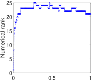
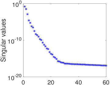
Fig. 1: Results for Example 1 for $(\alpha,\beta)=(1.5,1.5)$ and $N=M=200$. Left: Numerical rank of the LBDF2 solution as a function of $t$. Right: First $60$ singular values of the LBDF2 solution at $t=T$.

Example 1. In this example, the FGLE (1.1) is considered on $\Omega=[-10,10]\times[-10,10]$ with $u_{0}(x,y)=2\;\mathrm{sech}(x)\;\mathrm{sech}(y)e^{3\mathrm{\mathbf{i}}(x+y)}$, $\nu=\eta=\kappa=\xi=\gamma=1$ and $T=1$. For this case, the exact solution is unknown. The numerical solution ($(N,M)=(512,10000)$) computed by the linearized second-order backward differential (LBDF2) scheme [24] is used as the reference solution. Moreover, we denote the numerical solution obtained by the LBDF2 scheme [24] as the LBDF2 solution.

For rank $r\geq 3$, the relative errors in Table 1 decrease steadily with increasing the number of time steps $M$. In this table, the observed temporal convergence order is $1$ as expected. Table 2 reports the relative errors and the observed convergence order in space for different values of $\alpha$ and $\beta$. It shows that for fixed $M=10000$, the convergence order in space is indeed $2$ for $r\geq 3$. This is in good agreement with our theoretical analysis in Section 3.2. Fig. 1 (left) shows the rank of the LBDF2 solution with $(\alpha,\beta)=(1.5,1.5)$ and $N=M=200$. It can be observed that the effective rank of the solution is low. In Fig. 1 (right), we plot the first $60$ singular values of the LBDF2 solution at $T$. In Fig. 2, we compare the absolute values of the LBDF2 solution and our low-rank solution (rank $r=5$) at $t=T$ for different values of $\alpha$ and $\beta$. It can be seen that our proposed method is robust and accurate.

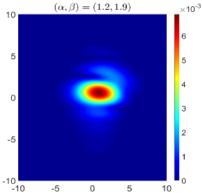
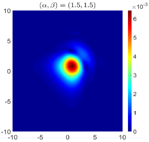
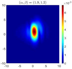
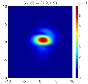
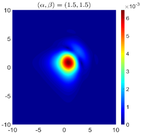
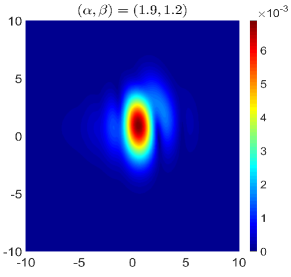
Fig. 2: Comparison of the absolute values of the LBDF2 solution and our low-rank solution at $t=T$ for $(N,M)=(512,200)$ and different values of $\alpha$ and $\beta$ for Example 1. Top row: The LBDF2 solution. Bottom row: The low-rank solution (rank $r=5$).

Table 1: Relative errors in Frobenius norm and observed temporal convergence orders for $N=512$ for Example 1.

		$r=1$		$r=2$		$r=3$		$r=4$		$r=5$
$(\alpha,\beta)$	$M$	$\textrm{relerr}(\tau,h)$	$\textrm{rate}_{\tau}$	$\textrm{relerr}(\tau,h)$	$\textrm{rate}_{\tau}$	$\textrm{relerr}(\tau,h)$	$\textrm{rate}_{\tau}$	$\textrm{relerr}(\tau,h)$	$\textrm{rate}_{\tau}$	$\textrm{relerr}(\tau,h)$	$\textrm{rate}_{\tau}$
(1.2, 1.9)	16	4.8609E-01	–	8.2522E-01	–	7.9346E-01	–	7.9240E-01	–	7.9253E-01	–
	64	5.3468E-01	-0.0687	2.0577E-01	1.0019	2.0557E-01	0.9743	2.0455E-01	0.9769	2.0499E-01	0.9755
	256	5.7709E-01	-0.0551	5.2778E-02	0.9815	5.1313E-02	1.0011	5.0386E-02	1.0107	5.0491E-02	1.0107
	1024	5.8871E-01	-0.0144	2.4422E-02	0.5559	1.3848E-02	0.9448	1.2499E-02	1.0056	1.2581E-02	1.0024
(1.5, 1.5)	16	5.5049E-01	–	7.9464E-01	–	7.6149E-01	–	7.5911E-01	–	7.5953E-01	–
	64	6.4759E-01	-0.1172	1.9941E-01	0.9973	1.9988E-01	0.9648	1.9839E-01	0.9680	1.9883E-01	0.9668
	256	6.9229E-01	-0.0481	5.4117E-02	0.9408	5.0664E-02	0.9901	4.9256E-02	1.0050	4.9399E-02	1.0045
	1024	7.0413E-01	-0.0122	3.0728E-02	0.4083	1.4516E-02	0.9017	1.2248E-02	1.0039	1.2361E-02	0.9993
(1.7, 1.3)	16	5.2921E-01	–	7.8605E-01	–	7.5265E-01	–	7.5042E-01	–	7.5024E-01	–
	64	6.0475E-01	-0.0962	1.9632E-01	1.0007	1.9643E-01	0.9690	1.9513E-01	0.9716	1.9547E-01	0.9702
	256	6.4751E-01	-0.0493	5.2519E-02	0.9511	4.9500E-02	0.9943	4.8334E-02	1.0067	4.8461E-02	1.0060
	1024	6.5899E-01	-0.0127	2.8515E-02	0.4406	1.3823E-02	0.9202	1.2008E-02	1.0045	1.2113E-02	1.0001
(1.9, 1.2)	16	4.9746E-01	–	8.3250E-01	–	7.9540E-01	–	7.9353E-01	–	7.9298E-01	–
	64	5.3481E-01	-0.0522	2.0620E-01	1.0067	2.0586E-01	0.9750	2.0476E-01	0.9772	2.0499E-01	0.9759
	256	5.7706E-01	-0.0548	5.2760E-02	0.9833	5.1371E-02	1.0013	5.0393E-02	1.0113	5.0492E-02	1.0107
	1024	5.8870E-01	-0.0144	2.4418E-02	0.5557	1.3867E-02	0.9446	1.2499E-02	1.0057	1.2581E-02	1.0024

Table 2: Relative errors in Frobenius norm and observed spatial convergence orders for $M=10000$ for Example 1.

		$r=1$		$r=2$		$r=3$		$r=4$		$r=5$
$(\alpha,\beta)$	$N$	$\textrm{relerr}(\tau,h)$	$\textrm{rate}_{h}$	$\textrm{relerr}(\tau,h)$	$\textrm{rate}_{h}$	$\textrm{relerr}(\tau,h)$	$\textrm{rate}_{h}$	$\textrm{relerr}(\tau,h)$	$\textrm{rate}_{h}$	$\textrm{relerr}(\tau,h)$	$\textrm{rate}_{h}$
(1.2, 1.9)	32	7.1496E-01	–	6.0075E-01	–	6.0033E-01	–	6.0079E-01	–	6.0069E-01	–
	64	5.8194E-01	0.2970	1.2508E-01	2.2639	1.2512E-01	2.2624	1.2478E-01	2.2675	1.2482E-01	2.2668
	128	5.8821E-01	-0.0155	3.5052E-02	1.8353	2.9685E-02	2.0755	2.8836E-02	2.1134	2.8893E-02	2.1111
	256	5.9137E-01	-0.0077	2.2788E-02	0.6212	7.9685E-03	1.8974	6.1959E-03	2.2185	6.2558E-03	2.2075
(1.5, 1.5)	32	8.2826E-01	–	6.2358E-01	–	6.2338E-01	–	6.2391E-01	–	6.2380E-01	–
	64	6.9735E-01	0.2482	1.2391E-01	2.3313	1.2393E-01	2.3306	1.2330E-01	2.3392	1.2337E-01	2.3381
	128	7.0396E-01	-0.0136	3.8797E-02	1.6753	2.9802E-02	2.0560	2.8319E-02	2.1223	2.8406E-02	2.1187
	256	7.0691E-01	-0.0060	2.9772E-02	0.3820	9.2925E-03	1.6813	6.1664E-03	2.1993	6.2448E-03	2.1855
(1.7, 1.3)	32	7.9484E-01	–	6.2588E-01	–	6.2572E-01	–	6.2618E-01	–	6.2608E-01	–
	64	6.5274E-01	0.2842	1.2632E-01	2.3088	1.2627E-01	2.3090	1.2579E-01	2.3156	1.2585E-01	2.3146
	128	6.5868E-01	-0.0131	3.7824E-02	1.7397	3.0045E-02	2.0713	2.8901E-02	2.1218	2.8976E-02	2.1188
	256	6.6165E-01	-0.0065	2.7462E-02	0.4619	8.6706E-03	1.7929	6.2136E-03	2.2176	6.2862E-03	2.2046
(1.9, 1.2)	32	7.1495E-01	–	6.0075E-01	–	6.0033E-01	–	6.0079E-01	–	6.0069E-01	–
	64	5.8194E-01	0.2970	1.2507E-01	2.2640	1.2512E-01	2.2624	1.2478E-01	2.2675	1.2482E-01	2.2668
	128	5.8821E-01	-0.0155	3.5052E-02	1.8352	2.9686E-02	2.0755	2.8836E-02	2.1134	2.8893E-02	2.1111
	256	5.9137E-01	-0.0077	2.2788E-02	0.6212	7.9705E-03	1.8970	6.1959E-03	2.2185	6.2558E-03	2.2075

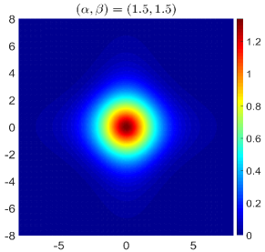
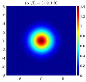
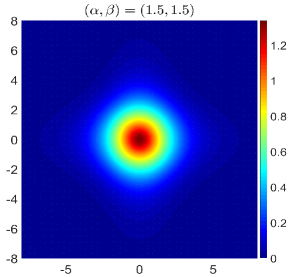
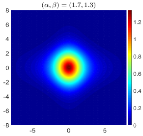
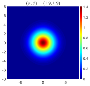
Fig. 3: Comparison of the absolute values of the LBDF2 solution and our low-rank solution at $t=T$ for $(N,M)=(512,200)$ and different values of $\alpha$ and $\beta$ for Example 2. Top row: The LBDF2 solution. Bottom row: The low-rank solution (rank $r=8$).

Example 2. In this example, in Eq. (1.1), we choose $\nu=\kappa=1$, $\eta=0.5$, $\xi=-5$, $\gamma=3$, $\Omega=[-8,8]\times[-8,8]$, $T=1$ and the initial value $u_{0}(x,y)=e^{-2\left(x^{2}+y^{2}\right)}e^{\mathrm{\mathbf{i}}S_{0}}$, where $S_{0}=\frac{1}{e^{x+y}+e^{-(x+y)}}$. The exact solution in this case is unknown. Similar to Example 1, we choose the LBDF2 solution with $(N,M)=(512,10000)$ as the reference solution.

Table 3 lists the errors and the observed temporal convergence orders. From this table, we can see that for fixed $N=512$ and $r\geq 6$, the observed temporal convergence order is $1$. In Table 4, for $r=8$, the observed spatial convergence order is $2$. In a word, these numerical results are consistent with the theoretical result in Section 3.2. Fig. 3 compares the absolute values of the LBDF2 solution and the low-rank solution ($r=8$) for different values of $\alpha$ and $\beta$. Moreover, if the rank $r\geq 8$, the errors are only slightly different and the convergence order will not improve significantly.

Table 3: Relative errors in Frobenius norm and observed temporal convergence orders for $N=512$ for Example 2.

		$r=1$		$r=2$		$r=4$		$r=6$		$r=8$
$(\alpha,\beta)$	$M$	$\textrm{relerr}(\tau,h)$	$\textrm{rate}_{\tau}$	$\textrm{relerr}(\tau,h)$	$\textrm{rate}_{\tau}$	$\textrm{relerr}(\tau,h)$	$\textrm{rate}_{\tau}$	$\textrm{relerr}(\tau,h)$	$\textrm{rate}_{\tau}$	$\textrm{relerr}(\tau,h)$	$\textrm{rate}_{\tau}$
(1.2, 1.9)	16	2.0955E-01	–	2.0940E-01	–	8.9892E-02	–	8.9162E-02	–	8.9135E-02	–
	64	1.9990E-01	0.0340	1.6160E-01	0.1869	2.5814E-02	0.9000	2.1950E-02	1.0111	2.1913E-02	1.0121
	256	2.0063E-01	-0.0026	1.5059E-01	0.0509	1.4928E-02	0.3951	5.5422E-03	0.9928	5.4473E-03	1.0041
	1024	2.0100E-01	-0.0013	1.4999E-01	0.0029	1.4018E-02	0.0454	1.6603E-03	0.8695	1.3588E-03	1.0016
(1.5, 1.5)	16	2.0938E-01	–	2.0924E-01	–	8.8782E-02	–	8.8147E-02	–	8.8130E-02	–
	64	2.0016E-01	0.0325	1.7916E-01	0.1120	2.5573E-02	0.8978	2.1698E-02	1.0112	2.1669E-02	1.0120
	256	2.0096E-01	-0.0029	1.5866E-01	0.0877	1.4931E-02	0.3882	5.4758E-03	0.9932	5.3878E-03	1.0039
	1024	2.0134E-01	-0.0014	1.5945E-01	-0.0036	1.4059E-02	0.0434	1.6403E-03	0.8696	1.3444E-03	1.0014
(1.7, 1.3)	16	2.1149E-01	–	2.1135E-01	–	8.9162E-02	–	8.8495E-02	–	8.8470E-02	–
	64	2.0198E-01	0.0332	1.6305E-01	0.1872	2.5737E-02	0.8963	2.1780E-02	1.0113	2.1745E-02	1.0123
	256	2.0270E-01	-0.0026	1.5353E-01	0.0434	1.5076E-02	0.3858	5.4999E-03	0.9928	5.4059E-03	1.0040
	1024	2.0306E-01	-0.0013	1.5552E-01	-0.0093	1.4197E-02	0.0433	1.6549E-03	0.8663	1.3484E-03	1.0016
(1.9, 1.2)	16	2.0979E-01	–	2.0964E-01	–	8.9854E-02	–	8.9167E-02	–	8.9134E-02	–
	64	1.9999E-01	0.0345	1.5760E-01	0.2058	2.5825E-02	0.8994	2.1951E-02	1.0111	2.1913E-02	1.0121
	256	2.0066E-01	-0.0024	1.4966E-01	0.0373	1.4938E-02	0.3949	5.5426E-03	0.9928	5.4473E-03	1.0041
	1024	2.0101E-01	-0.0013	1.5024E-01	-0.0028	1.4021E-02	0.0457	1.6605E-03	0.8695	1.3588E-03	1.0016

Table 4: Relative errors in Frobenius norm and observed spatial convergence orders for $M=10000$ for Example 2.

		$r=1$		$r=2$		$r=4$		$r=6$		$r=8$
$(\alpha,\beta)$	$N$	$\textrm{relerr}(\tau,h)$	$\textrm{rate}_{h}$	$\textrm{relerr}(\tau,h)$	$\textrm{rate}_{h}$	$\textrm{relerr}(\tau,h)$	$\textrm{rate}_{h}$	$\textrm{relerr}(\tau,h)$	$\textrm{rate}_{h}$	$\textrm{relerr}(\tau,h)$	$\textrm{rate}_{h}$
(1.2, 1.9)	32	2.2126E-01	–	1.8457E-01	–	3.7148E-02	–	3.4214E-02	–	3.4212E-02	–
	64	2.0525E-01	0.1084	1.6523E-01	0.1597	1.6935E-02	1.1333	9.3369E-03	1.8736	9.2804E-03	1.8822
	128	2.0204E-01	0.0227	1.6095E-01	0.0379	1.4196E-02	0.2545	2.4582E-03	1.9253	2.2641E-03	2.0352
	256	2.0130E-01	0.0053	1.5971E-01	0.0112	1.3986E-02	0.0215	1.0737E-03	1.1950	5.2148E-04	2.1183
(1.5, 1.5)	32	2.2202E-01	–	1.8081E-01	–	3.5474E-02	–	3.2514E-02	–	3.2513E-02	–
	64	2.0562E-01	0.1107	1.5709E-01	0.2029	1.6569E-02	1.0983	8.6606E-03	1.9085	8.6039E-03	1.9180
	128	2.0239E-01	0.0228	1.6308E-01	-0.0540	1.4206E-02	0.2220	2.3027E-03	1.9111	2.1004E-03	2.0343
	256	2.0164E-01	0.0054	1.5177E-01	0.1037	1.4030E-02	0.0180	1.0497E-03	1.1333	4.8398E-04	2.1176
(1.7, 1.3)	32	2.2395E-01	–	1.9556E-01	–	3.6112E-02	–	3.3115E-02	–	3.3112E-02	–
	64	2.0741E-01	0.1107	1.6221E-01	0.2697	1.6822E-02	1.1021	8.8906E-03	1.8971	8.8319E-03	1.9066
	128	2.0412E-01	0.0231	1.6714E-01	-0.0432	1.4352E-02	0.2291	2.3603E-03	1.9133	2.1549E-03	2.0351
	256	2.0337E-01	0.0053	1.5975E-01	0.0652	1.4167E-02	0.0187	1.0696E-03	1.1419	4.9634E-04	2.1182
(1.9, 1.2)	32	2.2126E-01	–	1.8671E-01	–	3.7143E-02	–	3.4214E-02	–	3.4212E-02	–
	64	2.0525E-01	0.1084	1.7556E-01	0.0888	1.6936E-02	1.1330	9.3369E-03	1.8736	9.2804E-03	1.8822
	128	2.0204E-01	0.0227	1.5858E-01	0.1468	1.4196E-02	0.2546	2.4582E-03	1.9253	2.2641E-03	2.0352
	256	2.0130E-01	0.0053	1.6113E-01	-0.0230	1.3986E-02	0.0215	1.0737E-03	1.1950	5.2148E-04	2.1183

5 Concluding remarks

In this paper, we propose a numerical integration method based on a dynamical low-rank approximation for solving the 2D space fractional Ginzburg-Landau equations (1.1). First, we use a second-order difference method to approximate the two Riesz fractional derivatives. From this, the matrix differential equation (2.3) is obtained. Next, we split Eq. (2.3) into a stiff linear part and a nonstiff (nonlinear) part (see Eqs. (2.4) and (2.5)), and then apply a dynamical low-rank approach. The convergence of our proposed method is studied in Section 3. Numerical examples strongly support the theoretical result which is given in Theorem 3.2. Based on this work, three future research directions are suggested:

• Extension of our method to other problems such as space fractional Schrödinger equations [28];

• For solving higher-dimensional version of (1.1), we suggest considering the dynamical tensor approximation proposed in [38, 39];

• Design some fast implementations (e.g., a parallel version) of our method.

References

References

- [1] A. C. Newell, J. A. Whitehead, Finite bandwidth, finite amplitude convection, J. Fluid Mech. 38 (1969) 279–303.
- [2] C. G. Lange, A. C. Newell, A stability criterion for envelope equations, SIAM J. Appl. Math. 27 (1974) 441–456.
- [3] L. A. Segel, Distant side-walls cause slow amplitude modulation of cellular convection, J. Fluid Mech. 38 (1969) 203–224.
- [4] K. Stewartson, J. Stuart, A non-linear instability theory for a wave system in plane Poiseuille flow, J. Fluid Mech. 48 (1971) 529–545.
- [5] Q. Du, M. D. Gunzburger, J. S. Peterson, Analysis and approximation of the Ginzburg-Landau model of superconductivity, SIAM Rev. 34 (1992) 54–81.
- [6] S. J. Chapman, S. D. Howison, J. R. Ockendon, Macroscopic models for superconductivity, SIAM Rev. 34 (1992) 529–560.
- [7] V. E. Tarasov, G. M. Zaslavsky, Fractional Ginzburg–Landau equation for fractal media, Physica A 354 (2005) 249–261.
- [8] V. E. Tarasov, G. M. Zaslavsky, Fractional dynamics of coupled oscillators with long-range interaction, Chaos 16 (2006) 023110. doi:10.1063/1.2197167.
- [9] A. V. Milovanov, J. J. Rasmussen, Fractional generalization of the Ginzburg–Landau equation: an unconventional approach to critical phenomena in complex media, Phys. Lett. A 337 (2005) 75–80.
- [10] A. Mvogo, A. Tambue, G. H. Ben-Bolie, T. C. Kofané, Localized numerical impulse solutions in diffuse neural networks modeled by the complex fractional Ginzburg–Landau equation, Commun. Nonlinear Sci. Numer. Simul. 39 (2016) 396–410.
- [11] V. E. Tarasov, Psi-series solution of fractional Ginzburg–Landau equation, J. Phys. A-Math. Theor. 39 (2006) 8395–8407.
- [12] X. Pu, B. Guo, Well-posedness and dynamics for the fractional Ginzburg-Landau equation, Appl. Anal. 92 (2013) 318–334.
- [13] B. Guo, Z. Huo, Well-posedness for the nonlinear fractional Schrödinger equation and inviscid limit behavior of solution for the fractional Ginzburg-Landau equation, Fract. Calc. Appl. Anal. 16 (2013) 226–242.
- [14] H. Lu, S. Lü, Z. Feng, Asymptotic dynamics of 2D fractional complex Ginzburg–Landau equation, Int. J. Bifurcation Chaos 23 (2013) 1350202. doi:10.1142/S0218127413502027.
- [15] V. Millot, Y. Sire, On a fractional Ginzburg–Landau equation and 1/2-harmonic maps into spheres, Arch. Ration. Mech. Anal. 215 (2015) 125–210.
- [16] P. Wang, C. Huang, An implicit midpoint difference scheme for the fractional Ginzburg–Landau equation, J. Comput. Phys. 312 (2016) 31–49.
- [17] Z.-P. Hao, Z.-Z. Sun, A linearized high-order difference scheme for the fractional Ginzburg–Landau equation, Numer. Meth. Part Differ. Equ. 33 (2017) 105–124.
- [18] M. Li, C. Huang, An efficient difference scheme for the coupled nonlinear fractional Ginzburg–Landau equations with the fractional Laplacian, Numer. Meth. Part. Differ. Equ. 35 (2019) 394–421.
- [19] L. Zhang, Q. Zhang, H.-W. Sun, Exponential Runge–Kutta method for two-dimensional nonlinear fractional complex Ginzburg–Landau equations, J. Sci. Comput. 83 (2020) 59. doi:10.1007/s10915-020-01240-x.
- [20] Z. Zhang, M. Li, Z. Wang, A linearized Crank–Nicolson Galerkin FEMs for the nonlinear fractional Ginzburg–Landau equation, Appl. Anal. 98 (2019) 2648–2667.
- [21] M. Li, C. Huang, N. Wang, Galerkin finite element method for the nonlinear fractional Ginzburg–Landau equation, Appl. Numer. Math. 118 (2017) 131–149.
- [22] N. Wang, C. Huang, An efficient split-step quasi-compact finite difference method for the nonlinear fractional Ginzburg–Landau equations, Comput. Math. Appl. 75 (2018) 2223–2242.
- [23] D. He, K. Pan, An unconditionally stable linearized difference scheme for the fractional Ginzburg-Landau equation, Numer. Algorithms 79 (2018) 899–925.
- [24] Q. Zhang, X. Lin, K. Pan, Y. Ren, Linearized ADI schemes for two-dimensional space-fractional nonlinear Ginzburg–Landau equation, Comput. Math. Appl. 80 (2020) 1201–1220.
- [25] O. Koch, C. Lubich, Dynamical low-rank approximation, SIAM J. Matrix Anal. Appl. 29 (2007) 434–454.
- [26] R. Gorenflo, F. Mainardi, Random walk models for space-fractional diffusion processes, Fract. Calc. Appl. Anal. 1 (1998) 167–191.
- [27] P. Wang, C. Huang, An energy conservative difference scheme for the nonlinear fractional Schrödinger equations, J. Comput. Phys. 293 (2015) 238–251.
- [28] X. Zhao, Z.-Z. Sun, Z.-P. Hao, A fourth-order compact ADI scheme for two-dimensional nonlinear space fractional Schrödinger equation, SIAM J. Sci. Comput. 36 (2014) A2865–A2886.
- [29] D. Wang, A. Xiao, W. Yang, A linearly implicit conservative difference scheme for the space fractional coupled nonlinear Schrödinger equations, J. Comput. Phys. 272 (2014) 644–655.
- [30] S. Zhai, D. Wang, Z. Weng, X. Zhao, Error analysis and numerical simulations of Strang splitting method for space fractional nonlinear Schrödinger equation, J. Sci. Comput. 81 (2019) 965–989.
- [31] M. Li, C. Huang, W. Ming, A relaxation-type Galerkin FEM for nonlinear fractional Schrödinger equations, Numer. Algorithms 83 (2020) 99–124.
- [32] P. A. M. Dirac, The Principles of Quantum Mechanics, 4th Edition, Oxford University Press, Oxford, 1981.
- [33] C. Lubich, From Quantum to Classical Molecular Dynamics: Reduced Models and Numerical Analysis, European Mathematical Society, Zürich, 2008.
- [34] A. Nonnenmacher, C. Lubich, Dynamical low-rank approximation: applications and numerical experiments, Math. Comput. Simul. 79 (2008) 1346–1357.
- [35] C. Lubich, I. V. Oseledets, A projector-splitting integrator for dynamical low-rank approximation, BIT 54 (2014) 171–188.
- [36] E. Kieri, C. Lubich, H. Walach, Discretized dynamical low-rank approximation in the presence of small singular values, SIAM J. Numer. Anal. 54 (2016) 1020–1038.
- [37] A. Ostermann, C. Piazzola, H. Walach, Convergence of a low-rank Lie-Trotter splitting for stiff matrix differential equations, SIAM J. Numer. Anal. 57 (2019) 1947–1966.
- [38] O. Koch, C. Lubich, Dynamical tensor approximation, SIAM J. Matrix Anal. Appl. 31 (2010) 2360–2375.
- [39] C. Lubich, T. Rohwedder, R. Schneider, B. Vandereycken, Dynamical approximation by hierarchical Tucker and tensor-train tensors, SIAM J. Matrix Anal. Appl. 34 (2013) 470–494.
- [40] L. Einkemmer, C. Lubich, A low-rank projector-splitting integrator for the Vlasov-Poisson equation, SIAM J. Sci. Comput. 40 (2018) B1330–B1360.
- [41] L. Einkemmer, C. Lubich, A quasi-conservative dynamical low-rank algorithm for the Vlasov equation, SIAM J. Sci. Comput. 41 (2019) B1061–B1081.
- [42] L. Einkemmer, A low-rank algorithm for weakly compressible flow, SIAM J. Sci. Comput. 41 (2019) A2795–A2814.
- [43] L. Grasedyck, D. Kressner, C. Tobler, A literature survey of low-rank tensor approximation techniques, GAMM-Mitt. 36 (2013) 53–78.
- [44] C. Çelik, M. Duman, Crank–Nicolson method for the fractional diffusion equation with the Riesz fractional derivative, J. Comput. Phys. 231 (2012) 1743–1750.
- [45] A. H. Al-Mohy, N. J. Higham, Computing the action of the matrix exponential, with an application to exponential integrators, SIAM J. Sci. Comput. 33 (2011) 488–511.
- [46] M. Caliari, P. Kandolf, A. Ostermann, S. Rainer, The Leja method revisited: Backward error analysis for the matrix exponential, SIAM J. Sci. Comput. 38 (2016) A1639–A1661.
- [47] Y. Saad, Analysis of some Krylov subspace approximations to the matrix exponential operator, SIAM J. Numer. Anal. 29 (1992) 209–228.
- [48] S. T. Lee, H.-K. Pang, H.-W. Sun, Shift-invert Arnoldi approximation to the Toeplitz matrix exponential, SIAM J. Sci. Comput. 32 (2010) 774–792.
- [49] U. Helmke, J. B. Moore, Optimization and Dynamical Systems, Springer-Verlag, London, 1994.
- [50] H. Sun, Z.-Z. Sun, G.-H. Gao, Some high order difference schemes for the space and time fractional Bloch–Torrey equations, Appl. Math. Comput. 281 (2016) 356–380.