Unknotting numbers and crossing numbers of spatial embeddings of a planar graph

Abstract.

It is known that the unknotting number $u(L)$ of a link $L$ is less than or equal to half the crossing number $c(L)$ of $L$. We show that there are a planar graph $G$ and its spatial embedding $f$ such that the unknotting number $u(f)$ of $f$ is greater than half the crossing number $c(f)$ of $f$. We study relations between unknotting number and crossing number of spatial embedding of a planar graph in general.

1. Introduction

Let $L$ be a link in the $3$-dimensional Euclidean space ${\mathbb{R}}^{3}$. Let $c(L)$ be the crossing number of $L$, that is, the minimal number of crossing points among all regular diagrams of $L$. Let $u(L)$ be the unknotting number of $L$, that is, the minimal number of crossing changes from $L$ to a trivial link. It is well-known that $u(L)$ is less than or equal to half of $c(L)$. See for example [7]. In this paper we show that this is not extended to spatial embeddings of planar graphs. We also show that this is extended to spatial embeddings of trivializable planar graphs.

Let $G$ be a planar graph, that is, $G$ has an embedding into the plane ${\mathbb{R}}^{2}$, or equivalently, into the $2$-sphere ${\mathbb{S}}^{2}$. We denote the set of all vertices by ${\rm V}(G)$ and the set of all edges by ${\rm E}(G)$. An embedding $f:G\to{\mathbb{R}}^{3}$ is said to be a spatial embedding of $G$ and its image $f(G)$ is said to be a spatial graph. Let ${\rm SE}(G)$ be the set of all spatial embeddings of $G$. Let $\pi:{\mathbb{R}}^{3}\to{\mathbb{R}}^{2}$ be a natural projection defined by $\pi(x,y,z)=(x,y)$. We may assume up to ambient isotopy of ${\mathbb{R}}^{3}$ that $f\in{\rm SE}(G)$ is in general position with respect to $\pi$. Namely the composition map $\pi\circ f:G\to{\mathbb{R}}^{2}$ is a generic immersion. Here a continuous map $\varphi:G\to{\mathbb{R}}^{2}$ is said to be a generic immersion if it has only finitely many multiple points each of which is a transversal double point of an edge or two edges of $G$. Such a double point is said to be a crossing point, or simply a crossing. The set of all crossings of $\varphi$ is denoted by ${\mathcal{C}}(\varphi)$ and the number of crossings of $\varphi$ is denoted by $c(\varphi)=|{\mathcal{C}}(\varphi)|$. A regular diagram, or simply a diagram $D$ of $f\in{\rm SE}(G)$ is the image $\pi\circ f(G)\subset{\mathbb{R}}^{2}$ together with vertex/edge labels and over/under information at each crossing point. The set of all crossing points of $D$ is denoted by ${\mathcal{C}}(D)$ and the number of crossings of $D$ is denoted by $c(D)=|{\mathcal{C}}(D)|$.

An element $t\in{\rm SE}(G)$ is said to be trivial, or unknotted, if there is a $2$-sphere $S$ embedded in ${\mathbb{R}}^{3}$ such that $t(G)\subset S$. It is known in [2] that any two trivial embeddings of a planar graph are ambient isotopic. Therefore unknotting number is naturally extended to spatial embeddings of planar graphs as follows. For $f\in{\rm SE}(G)$, the unknotting number $u(f)$ of $f$ is defined to be the minimal number of crossing changes from $f$ to a trivial embedding of $G$. The crossing number $c(f)$ of $f$ is defined to be the minimal number of crossing points among all regular diagrams of spatial embeddings that are ambient isotopic to $f$.

In comparison to link case stated above, we will show that there are a planar graph $G$ and a spatial embedding $f$ of $G$ such that $u(f)$ is greater than half of $c(f)$. Before giving an infinite sequence of such examples in Theorem 1-1, we exhibit the first term of the sequence here. Let $P_{3}$ be the cube graph and $f_{3}\in{\rm SE}(P_{3})$ a spatial embedding of $P_{3}$ illustrated in Figure 1.1. Since $f_{3}(P_{3})$ contains a trefoil knot whose crossing number is $3$, we have $c(f_{3})=3$. The cube graph $P_{3}$ contains exactly $3$ pairs of mutually disjoint cycles. Each of them is a pair of parallel squares of the cube. Each of them forms a Hopf link in $f_{3}(P_{3})$ as illustrated in Figure 1.1. Therefore $f_{3}(P_{3})$ contains exactly $3$ Hopf links. Suppose that a crossing change is performed between two edges of $P_{3}$. Then only links that contain both of them may be changed. Since each edge of the cube is contained in exactly two squares, a crossing change may change at most $2$ Hopf links. Therefore at least one Hopf link remains after a crossing change and we have $u(f_{3})>1$. We will show later that $u(f_{3})\leq 2$. Therefore $u(f_{3})=2$ and it is greater than half of $c(f_{3})=3$.

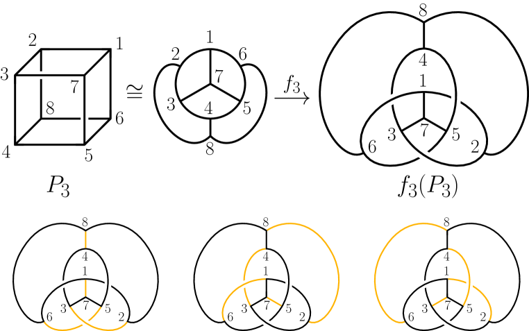
Figure 1.1. An example

Let $n\in{\mathbb{N}}$ be a natural number. Let $P_{2n+1}$ be a planar graph and $f_{2n+1}\in{\rm SE}(P_{2n+1})$ a spatial embedding of $P_{2n+1}$ illustrated in Figure 1.2. Since $f_{2n+1}(P_{2n+1})$ contains a $(2,2n+1)$-torus knot whose crossing number is $2n+1$, we have $c(f_{2n+1})=2n+1$. We have the following theorem whose proof will be given in §2.

Theorem 1-1.

Let $n\in{\mathbb{N}}$ be a natural number. Then $u(f_{2n+1})=2n$.

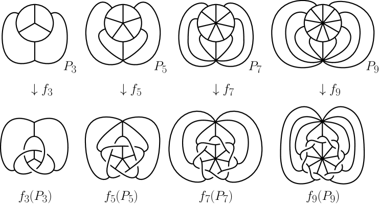
Figure 1.2. Examples

Now we explain the reason why it happens for these planar graphs. First we review the proof of $\displaystyle{u(L)\leq\frac{1}{2}c(L)}$ for a link $L$. It is well-known that every diagram of a link turns into a diagram of a trivial link by changing some of their crossings. Let $D$ be a diagram of $L$ with $c(D)=c(L)$. Then there is a subset $A$ of ${\mathcal{C}}(D)$ such that changing all crossings in $A$ turns $D$ to a diagram $T$ of a trivial link. Let $S$ be a diagram obtained from $D$ by changing all crossings in $B={\mathcal{C}}(D)\setminus A$. Note that $S$ is obtained from $T$ by changing all crossings of $T$. Therefore $S$ is a diagram of a mirror image of a trivial link. A mirror image of a trivial link is again a trivial link. Therefore $S$ is also a diagram of a trivial link. Thus we have $\displaystyle{u(L)\leq{\rm min}\{|A|,|B|\}\leq\frac{1}{2}c(D)=\frac{1}{2}c(L)}$.

However there are a planar graph $G$ and a generic immersion $\varphi:G\to{\mathbb{R}}^{2}$ such that every spatial embedding $f$ of $G$ with $\pi\circ f=\varphi$ is not trivial [6]. Such a generic immersion or its image is said to be a knotted projection. The projection $\pi\circ f_{3}(P_{3})$ illustrated in Figure 1.3 is a knotted projection first appeared in [4]. Since $c(\pi\circ f_{3})=3$ there are $2^{3}=8$ diagrams coming from it. Up to mirror image and $2\pi/3$-rotation on the sphere ${\mathbb{S}}^{2}={\mathbb{R}}^{2}\cup\{\infty\}$ they are the diagrams illustrated in Figure 1.3. One of them contains three Hopf links and the other contains one Hopf link.

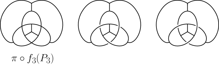
Figure 1.3. A knotted projection and diagrams coming from it

A planar graph is said to be trivializable if it has no knotted projections. The set of all trivializable planar graphs is closed under minor reduction [6]. A certain class of planar graphs are known to be trivializable [6] [4] [5] [3].

For a spatial embedding of a trivializable planar graph, the same argument as for a link works, and we have the following proposition.

Proposition 1-2.

Let $G$ be a trivializable planar graph and $f:G\to{\mathbb{R}}^{3}$ a spatial embedding of $G$. Then $\displaystyle{u(f)\leq\frac{1}{2}c(f)}$.

Then we are interested in the relation between unknotting number and crossing number of spatial embedding of a planar graph that holds in general.

Theorem 1-3.

Let $G$ be a planar graph. Then there exist real numbers $A$ and $B$ with the following property. For any spatial embedding $f:G\to{\mathbb{R}}^{3}$ of $G$, $\displaystyle{u(f)\leq A\cdot c(f)+B}$.

2. Proofs

Some estimations below of the unknotting numbers of spatial embeddings of a planar graph are given in [1]. In the following we give an estimation below based on an analysis of the changes of the linking numbers in a spatial graph.

Proof of Theorem 1-1. First we show $u(f_{2n+1})\leq 2n$. It is shown in Figure 2.1.

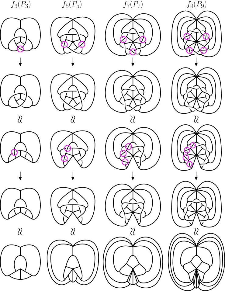
Figure 2.1. $u(f_{2n+1})\leq 2n$

Next we show $u(f_{2n+1})\geq 2n$. A prototype of the following proof is the proof of $u(f_{3})\geq 2$ given in §1. Let $C_{4n+2}$ be the $4n+2$-cycle of $P_{2n+1}$ such that $f_{2n+1}(C_{4n+2})$ is a $(2,2n+1)$-torus knot. We call $C_{4n+2}$ the equator of $P_{2n+1}$. Each edge of $C_{4n+2}$ is said to be an equatorial edge. Let $v_{N}$ and $v_{S}$ the vertices of $P_{2n+1}$ not on $C_{4n+2}$. We call $v_{N}$ the north pole and $v_{S}$ the south pole. An edge incident to $v_{N}$ (resp. $v_{S}$) is said to be a north spoke (resp. south spoke). In the following we consider the suffixes of vertices of $P_{2n+1}$ modulo $2n+1$. Let $u_{1},u_{2},\cdots,u_{2n+1}$ be the vertices on $C_{4n+2}$ that are adjacent to $v_{N}$ and $v_{1},v_{2},\cdots,v_{2n+1}$ the vertices on $C_{4n+2}$ that are adjacent to $v_{S}$. We may assume that these vertices are cyclically arranged on $C_{4n+2}$ as $u_{1},v_{n+2},u_{2},v_{n+3},\cdots,u_{2n+1},v_{n+1}$. Let $N_{i}$ be a $4$-cycle $u_{i}v_{i+n+1}u_{i+1}v_{N}u_{i}$ oriented by this cyclic order of vertices and $S_{i}$ a $4$-cycle $v_{i}u_{i+n+1}v_{i+1}v_{S}v_{i}$ oriented by this cyclic order of vertices for $i=1,2,\cdots,2n+1$. These cycles are the region cycles when $P_{2n+1}$ is embedded into the $2$-sphere ${\mathbb{S}}^{2}$. Let ${\mathcal{R}}_{2n+1}=\{N_{1},\cdots,N_{2n+1},S_{1},\cdots,S_{2n+1}\}$ and we call ${\mathcal{R}}_{2n+1}$ the region cycles of $P_{2n+1}$. The case $n=4$ is illustrated in Figure 2.2.

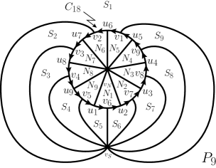
Figure 2.2. Cycles of $P_{9}$

For each spatial embedding $f$ of $P_{2n+1}$, we define the following integers. Here $\ell k(J,K)$ denotes the linking number of $J$ and $K$.

$$\ell_{1}(f) =\sum_{i=1}^{2n+1}\ell k(f(N_{i}),f(S_{i}))$$

$$\ell_{2}(f) =\sum_{i=1}^{2n+1}\ell k(f(N_{i}),f(S_{i+1}))+\sum_{i=1}^{2n+1}\ell k(f(N_{i}),f(S_{i-1}))$$

$$\ell_{3}(f) =\sum_{i=1}^{2n+1}\ell k(f(N_{i}),f(S_{i+2}))+\sum_{i=1}^{2n+1}\ell k(f(N_{i}),f(S_{i-2}))$$

$$\vdots$$

$$\ell_{n}(f) =\sum_{i=1}^{2n+1}\ell k(f(N_{i}),f(S_{i+n-1}))+\sum_{i=1}^{2n+1}\ell k(f(N_{i}),f(S_{i-n+1}))$$

Then we define an element ${\mathcal{L}}(f)$ of ${\mathbb{Z}}^{n}$ by ${\mathcal{L}}(f)=(\ell_{1}(f),\ell_{2}(f),\cdots,\ell_{n}(f))$. We will observe how ${\mathcal{L}}(f)$ changes under a crossing change. Note that a crossing change between two strands of the same component does not change the linking number of a two-component link. Therefore a crossing change between two strands of the same edge does not change any linking numbers. Also a crossing change between two mutually adjacent edges does not change any linking numbers. Therefore we consider crossing changes between two mutually disjoint edges. Note that each edge of $P_{2n+1}$ is contained in exactly two region cycles of $P_{2n+1}$. Therefore a crossing change between two mutually disjoint edges of $P_{2n+1}$ changes at most four linking numbers. First we show an example. Suppose that a crossing change is performed between edge $v_{N}u_{1}$ and edge $v_{S}v_{1}$. Taking crossing signs under cycle orientations into account, we see that each of $\ell k(f(N_{1}),f(S_{1}))$ and $\ell k(f(N_{2n+1}),f(S_{2n+1}))$ changes by $\pm 1$, each of $\ell k(f(N_{1}),f(S_{2n+1}))$ and $\ell k(f(N_{2n+1}),f(S_{1}))$ changes by $\mp 1$, and all other linking numbers are unchanged. Therefore ${\mathcal{L}}(f)$ changes by $\pm(2,-2,0,\cdots,0)$. In such a way we have a list of possible changes of ${\mathcal{L}}(f)$ under a crossing change as follows.

• Crossing changes between two equatorial edges

  $$\pm(2,0,\cdots,0),\pm(1,1,0,\cdots,0),\pm(0,2,0,\cdots,0),\pm(0,1,1,0,\cdots,0),$$

  $$\pm(0,0,2,0,\cdots,0),\pm(0,0,1,1,0,\cdots,0),\cdots\cdots,$$

  $$\pm(0,\cdots,0,2,0),\pm(0,\cdots,0,1,1),\pm(0,\cdots,0,2),\pm(0,\cdots,0,1)$$

• Crossing changes between an equatorial edge and a spoke

  $$\pm(1,-1,0,\cdots,0),\pm(0,1,-1,0,\cdots,0),\pm(0,0,1,-1,0,\cdots,0),$$

  $$\cdots\cdots,\pm(0,\cdots,0,1,-1,0),\pm(0,\cdots,0,1,-1),\pm(0,\cdots,0,1)$$

• Crossing changes between a north spoke and a south spoke

  $$\pm(2,-2,0,\cdots,0),\pm(1,-2,1,0,\cdots,0),\pm(0,1,-2,1,0,\cdots,0),$$

  $$\pm(0,0,1,-2,1,0,\cdots,0),\cdots\cdots,\pm(0,\cdots,0,1,-2,1,0),$$

  $$\pm(0,\cdots,0,1,-2,1),\pm(0,\cdots,0,1,-2),\pm(0,\cdots,0,1)$$

Let ${\mathcal{B}}_{2n+1}$ be a finite subset of ${\mathbb{Z}}^{n}$ consists of the following elements.

$$a_{1}=(2,0,\cdots,0),a_{2}=(0,2,0,\cdots,0),\cdots,a_{n}=(0,\cdots,0,2)$$

$$b_{1}=(1,1,0,\cdots,0),b_{2}=(0,1,1,0,\cdots,0),\cdots,b_{n-1}=(0,\cdots,0,1,1)$$

$$c_{1}=(1,-1,0,\cdots,0),c_{2}=(0,1,-1,0,\cdots,0),\cdots,c_{n-1}=(0,\cdots,0,1,-1)$$

$$d=e_{0}=(2,-2,0,\cdots,0)$$

$$e_{1}=(1,-2,1,0,\cdots,0),e_{2}=(0,1,-2,1,0,\cdots,0),\cdots,e_{n-2}=(0,\cdots,0,1,-2,1)$$

$$p=e_{n-1}=(0,\cdots,0,1,-2)$$

$$q=b_{n}=c_{n}=e_{n}=(0,\cdots,0,1)$$

We denote the $i$-th component of an element $v$ of ${\mathbb{Z}}^{n}$ by $v(i)$. Namely $v=(v(1),\cdots,v(n))$. Suppose that two spatial embeddings $f$ and $g$ of $P_{2n+1}$ are transformed into each other by $m$ times crossing changes. Then by the observation above we see that there is a map $\varphi:{\mathcal{B}}_{2n+1}\to{\mathbb{Z}}$ with $\displaystyle{\sum_{v\in{\mathcal{B}}_{2n+1}}|\varphi(v)|\leq m}$ such that

$${\mathcal{L}}(f)-{\mathcal{L}}(g)=\sum_{v\in{\mathcal{B}}_{2n+1}}\varphi(v)v.$$

From Figure 1.2 we see that ${\mathcal{L}}(f_{2n+1})=(2n+1,0,\cdots,0)$. Note that ${\mathcal{L}}(t_{2n+1})=(0,\cdots,0)$ where $t_{2n+1}$ is a trivial embedding of $P_{2n+1}$. We have seen above that $f_{2n+1}$ and $t_{2n+1}$ are transformed into each other by $2n$ times crossing changes as illustrated in Figure 2.1. All of them are performed between two equatorial edges. First $n$ crossing changes correspond to $n$ times $(2,0,\cdots,0)$. Next $n$ crossing changes corresponds to

$$(1,1,0,\cdots,0),-(0,1,1,0,\cdots,0),(0,0,1,1,0,\cdots,0),-(0,0,0,1,1,0,\cdots,0),\cdots,$$

$$(-1)^{n-3}(0,\cdots,0,1,1,0),(-1)^{n-2}(0,\cdots,0,1,1),(-1)^{n-1}(0,\cdots,0,1).$$

In fact the sum

$$n(2,0,\cdots,0)+(1,1,0,\cdots,0)-(0,1,1,0,\cdots,0)+(0,0,1,1,0,\cdots,0)$$

$$-(0,0,0,1,1,0,\cdots,0)+\cdots+(-1)^{n-3}(0,\cdots,0,1,1,0)$$

$$+(-1)^{n-2}(0,\cdots,0,1,1)+(-1)^{n-1}(0,\cdots,0,1)$$

is equal to $(2n+1,0,\cdots,0)={\mathcal{L}}(f_{2n+1})-{\mathcal{L}}(t_{2n+1})$.

The following claim assures that at least $2n$ crossing changes are necessary.

Claim. Let $\varphi:{\mathcal{B}}_{2n+1}\to{\mathbb{Z}}$ be a map with

$$\sum_{v\in{\mathcal{B}}_{2n+1}}\varphi(v)v=(2n+1,0,\cdots,0).$$

Then $\displaystyle{\sum_{v\in{\mathcal{B}}_{2n+1}}|\varphi(v)|\geq 2n.}$

We will show this claim step by step as follows.

Subclaim 1. Let $\varphi:{\mathcal{B}}_{2n+1}\to{\mathbb{Z}}$ be a map with

$$\sum_{v\in{\mathcal{B}}_{2n+1}}\varphi(v)v=(2n+1,*,\cdots,*).$$

Then $\displaystyle{\sum_{v\in{\mathcal{B}}_{2n+1}}|\varphi(v)|\geq n+1.}$ If $\displaystyle{\sum_{v\in{\mathcal{B}}_{2n+1}}|\varphi(v)|=n+1,}$ then $\displaystyle{\sum_{v\in{\mathcal{B}}_{2n+1}}\varphi(v)v(3)}$ is $0$ or $1$.

Proof. Note that $|v(1)|\leq 2$ for any $v\in{\mathcal{B}}_{2n+1}$. Therefore $\displaystyle{\sum_{v\in{\mathcal{B}}_{2n+1}}|\varphi(v)|\leq n}$ implies $\displaystyle{\sum_{v\in{\mathcal{B}}_{2n+1}}\varphi(v)v(1)\leq 2n<2n+1.}$ Thus we have $\displaystyle{\sum_{v\in{\mathcal{B}}_{2n+1}}|\varphi(v)|\geq n+1.}$ Suppose $\displaystyle{\sum_{v\in{\mathcal{B}}_{2n+1}}|\varphi(v)|=n+1.}$ Note that for $v\in{\mathcal{B}}_{2n+1}$, $v(1)=2$ if and only if $v\in\{a_{1},d\}$, $v(1)=1$ if and only if $v\in\{b_{1},c_{1},e_{1}\}$ and $v(1)=0$ otherwise. Then we see $\varphi(a_{1})+\varphi(d)=|\varphi(a_{1})|+|\varphi(d)|=n$ and $\varphi(b_{1})+\varphi(c_{1})+\varphi(e_{1})=|\varphi(b_{1})|+|\varphi(c_{1})|+|\varphi(e_{1})|=1$. Since $a_{1}(3)=d(3)=b_{1}(3)=c_{1}(3)=0$ and $e_{1}(3)=1$, we see that

$$\sum_{v\in{\mathcal{B}}_{2n+1}}\varphi(v)v(3) =\varphi(a_{1})a_{1}(3)+\varphi(d)d(3)+\varphi(b_{1})b_{1}(3)+\varphi(c_{1})c_{1}(3)+\varphi(e_{1})e_{1}(3)$$

is $0$ or $1$. $\Box$

Subclaim 2. Let $\varphi:{\mathcal{B}}_{2n+1}\to{\mathbb{Z}}$ be a map with

$$\sum_{v\in{\mathcal{B}}_{2n+1}}\varphi(v)v=(2n+1,0,*,\cdots,*).$$

Then $\displaystyle{\sum_{v\in{\mathcal{B}}_{2n+1}}|\varphi(v)|\geq n+2.}$ If $\displaystyle{\sum_{v\in{\mathcal{B}}_{2n+1}}|\varphi(v)|=n+2,}$ then $\displaystyle{\sum_{v\in{\mathcal{B}}_{2n+1}}\varphi(v)v(4)}$ is $0$, $1$ or $-1$.

Proof. By Subclaim 1 we have $\displaystyle{\sum_{v\in{\mathcal{B}}_{2n+1}}|\varphi(v)|\geq n+1.}$
Suppose $\displaystyle{\sum_{v\in{\mathcal{B}}_{2n+1}}|\varphi(v)|=n+1.}$ Then $\varphi(a_{1})+\varphi(d)=|\varphi(a_{1})|+|\varphi(d)|=n$ and $\varphi(b_{1})+\varphi(c_{1})+\varphi(e_{1})=|\varphi(b_{1})|+|\varphi(c_{1})|+|\varphi(e_{1})|=1$ as above. Since $a_{1}(2)=0,d(2)=-2,b_{1}(2)=1,c_{1}(2)=-1$ and $e_{1}(2)=-2$, we see that

$$\sum_{v\in{\mathcal{B}}_{2n+1}}\varphi(v)v(2) =\varphi(a_{1})a_{1}(2)+\varphi(d)d(2)+\varphi(b_{1})b_{1}(2)+\varphi(c_{1})c_{1}(2)+\varphi(e_{1})e_{1}(2)$$

is an odd number or a negative number, and cannot equal $0$. Therefore we have $\displaystyle{\sum_{v\in{\mathcal{B}}_{2n+1}}|\varphi(v)|\geq n+2.}$
Suppose $\displaystyle{\sum_{v\in{\mathcal{B}}_{2n+1}}|\varphi(v)|=n+2.}$ Suppose $\displaystyle{\sum_{v\in{\mathcal{B}}_{2n+1},v(4)\neq 0}|\varphi(v)|\geq 2.}$ Let $\psi:{\mathcal{B}}_{2n+1}\to{\mathbb{Z}}$ be a map defined by

$$\psi(v)=\begin{cases}\varphi(v)&(v(4)=0)\\ 0&(v(4)\neq 0).\end{cases}$$

Then we have $\displaystyle{\sum_{v\in{\mathcal{B}}_{2n+1}}|\psi(v)|\leq n.}$ Since $v(4)\neq 0$ implies $v(1)=0$, we have

$$\sum_{v\in{\mathcal{B}}_{2n+1}}\psi(v)v=(2n+1,*,\cdots,*).$$

This contradicts Subclaim 1. Therefore $\displaystyle{\sum_{v\in{\mathcal{B}}_{2n+1},v(4)\neq 0}|\varphi(v)|\leq 1.}$ Suppose that $u(4)\neq 0$ and $|\varphi(u)|=1$. Suppose that $u\neq e_{2}=(0,1,-2,1,0,\cdots,0)$. Then $u(1)=u(2)=0$. Let $\psi:{\mathcal{B}}_{2n+1}\to{\mathbb{Z}}$ be a map defined by

$$\psi(v)=\begin{cases}\varphi(v)&(v\neq u)\\ 0&(v=u).\end{cases}$$

Then we have $\displaystyle{\sum_{v\in{\mathcal{B}}_{2n+1}}|\psi(v)|=n+1}$ and

$$\sum_{v\in{\mathcal{B}}_{2n+1}}\psi(v)v=(2n+1,0,*,\cdots,*).$$

This is a contradiction. Therefore $u=(0,1,-2,1,0,\cdots,0)$ and $\displaystyle{\sum_{v\in{\mathcal{B}}_{2n+1}}\varphi(v)v(4)}=\pm 1$. $\Box$

Now we inductively show the subclaims for $3\leq k\leq n$.

Subclaim $k$. Let $\varphi:{\mathcal{B}}_{2n+1}\to{\mathbb{Z}}$ be a map with

$$\sum_{v\in{\mathcal{B}}_{2n+1}}\varphi(v)v=(2n+1,\underbrace{0,\cdots,0}_{k-1},*,\cdots,*).$$

Then $\displaystyle{\sum_{v\in{\mathcal{B}}_{2n+1}}|\varphi(v)|\geq n+k.}$
If $k\leq n-2$ and $\displaystyle{\sum_{v\in{\mathcal{B}}_{2n+1}}|\varphi(v)|=n+k,}$ then $\displaystyle{\sum_{v\in{\mathcal{B}}_{2n+1}}\varphi(v)v(k+2)}$ is $0$, $1$ or $-1$.

Proof. By Subclaim $k-1$ we have $\displaystyle{\sum_{v\in{\mathcal{B}}_{2n+1}}|\varphi(v)|\geq n+k-1.}$
Suppose $\displaystyle{\sum_{v\in{\mathcal{B}}_{2n+1}}|\varphi(v)|=n+k-1.}$ Note that the sum

$$\sum_{i=1}^{k}\left(\sum_{v\in{\mathcal{B}}_{2n+1}}\varphi(v)v(i)\right)=(2n+1)+\underbrace{0+\cdots+0}_{k-1}=2n+1$$

is odd. For $v\in{\mathcal{B}}_{2n+1}$, $\displaystyle{\sum_{i=1}^{k}v(i)}$ is odd if and only if $v\in\{b_{k},c_{k},e_{k-1},e_{k}\}$. Therefore there exist $u\in\{b_{k},c_{k},e_{k-1},e_{k}\}$ with $\varphi(u)\neq 0$. Let $\psi:{\mathcal{B}}_{2n+1}\to{\mathbb{Z}}$ be a map defined by

$$\psi(v)=\begin{cases}\varphi(v)&(v\neq u)\\ 0&(v=u).\end{cases}$$

Then we have $\displaystyle{\sum_{v\in{\mathcal{B}}_{2n+1}}|\psi(v)|\leq n+k-2.}$ Suppose $u\in\{b_{k},c_{k},e_{k}\}$. Then we see $u(i)=0$ for all $i\leq k-1$. Therefore we have

$$\sum_{v\in{\mathcal{B}}_{2n+1}}\psi(v)v=(2n+1,\underbrace{0,\cdots,0}_{k-2},*,\cdots,*).$$

This contradicts Subclaim $k-1$. Suppose $u=e_{k-1}$. Then we have

$$\sum_{v\in{\mathcal{B}}_{2n+1}}\psi(v)v=(2n+1,\underbrace{0,\cdots,0}_{k-3},-\varphi(u),-2\varphi(u),*,\cdots,*).$$

This contradicts Subclaim $k-2$ that asserts $\displaystyle{\sum_{v\in{\mathcal{B}}_{2n+1}}\psi(v)v(k)}$ is $0$, $1$ or $-1$. Therefore we have $\displaystyle{\sum_{v\in{\mathcal{B}}_{2n+1}}|\varphi(v)|\geq n+k.}$
Suppose $\displaystyle{\sum_{v\in{\mathcal{B}}_{2n+1}}|\varphi(v)|=n+k.}$ Suppose $\displaystyle{\sum_{v\in{\mathcal{B}}_{2n+1},v(k+2)\neq 0}|\varphi(v)|\geq 2.}$ Let $\psi:{\mathcal{B}}_{2n+1}\to{\mathbb{Z}}$ be a map defined by

$$\psi(v)=\begin{cases}\varphi(v)&(v(k+2)=0)\\ 0&(v(k+2)\neq 0).\end{cases}$$

Then we have $\displaystyle{\sum_{v\in{\mathcal{B}}_{2n+1}}|\psi(v)|\leq n+k-2.}$ Since $v(k+2)\neq 0$ implies $v(i)=0$ for all $i\leq k-1$, we have

$$\sum_{v\in{\mathcal{B}}_{2n+1}}\psi(v)v=(2n+1,\underbrace{0,\cdots,0}_{k-2},*,\cdots,*).$$

This contradicts Subclaim $k-1$. Therefore $\displaystyle{\sum_{v\in{\mathcal{B}}_{2n+1},v(k+2)\neq 0}|\varphi(v)|\leq 1.}$ Suppose that $u(k+2)\neq 0$ and $|\varphi(u)|=1$. Suppose that $u\neq e_{k}=(\underbrace{0,\cdots,0}_{k-1},1,-2,1,0,\cdots,0)$. Then $u(i)=0$ for all $i\leq k$. Let $\psi:{\mathcal{B}}_{2n+1}\to{\mathbb{Z}}$ be a map defined by

$$\psi(v)=\begin{cases}\varphi(v)&(v\neq u)\\ 0&(v=u).\end{cases}$$

Then we have $\displaystyle{\sum_{v\in{\mathcal{B}}_{2n+1}}|\psi(v)|=n+k-1}$ and

$$\sum_{v\in{\mathcal{B}}_{2n+1}}\psi(v)v=(2n+1,\underbrace{0,\cdots,0}_{k-1},*,\cdots,*).$$

This is a contradiction. Therefore we have $u=(\underbrace{0,\cdots,0}_{k-1},1,-2,1,0,\cdots,0)$ and $\displaystyle{\sum_{v\in{\mathcal{B}}_{2n+1}}\varphi(v)v(k+2)}=\pm 1$. $\Box$

Note that Subclaim $n$ is equal to Claim. Thus we have shown $u(f_{2n+1})\geq 2n$. $\Box$

Proof of Theorem 1-3. We choose and fix a spanning tree $T$ of $G$ and a vertex $v$ of $T$. We also choose a fixed embedding $G\subset{\mathbb{R}}^{2}$. Then we have an embedding of $T$ into ${\mathbb{R}}^{2}$ by $T\subset G\subset{\mathbb{R}}^{2}$. For a vertex $u$ of $G$, the degree of $u$ in $G$ is denoted by ${\rm deg}(u,G)$. For a vertex $u$ of $T$, the degree of $u$ in $T$ is denoted by ${\rm deg}(u,T)$. Note that ${\rm deg}(u,T)\leq{\rm deg}(u,G)$. Let $D$ be a diagram of $f$ with $c(D)=c(f)$. For each vertex $u$ of $T$ with ${\rm deg}(u,T)\geq 3$ we repeatedly perform the deformation of $D$ near $u$ illustrated in Figure 2.3 such that the cyclic order of the edges of $T$ incident to $u$ near $u$ coincides with that of $u$ in $T\subset G\subset{\mathbb{R}}^{2}$. Note that the deformation involves not only the edges of $T$ but all edges of $G$ incident to $u$. Each deformation increase the number of crossings by $1$. We will see that the increase of $c(D)$ is bounded above by a constant $b$ that depends only on $G$. Suppose that ${\rm deg}(u,G)$ is $2k_{u}+1$ or $2k_{u}+2$. Let $l_{u}={\rm deg}(u,T)$. We fix an edge of $T$ incident to $u$ and deform other edges of $T$ incident to $u$ so that the cyclic order of them is equal to that in $T\subset G\subset{\mathbb{R}}^{2}$. By the choice of turning right or left, at most $k_{u}$ times application of the deformation illustrated in Figure 2.3 is sufficient to move each edge into a designated position. Therefore we see that at most $k_{u}(l_{u}-1)$ times application of the deformation illustrated in Figure 2.3 is sufficient to change the cyclic order of the edges of $T$ incident to $u$. Therefore at most $b=\displaystyle{\sum_{u}k_{u}(l_{u}-1)}$ times application is sufficient. Thus the diagram $D$ is deformed into a diagram $D^{\prime}$ with $c(D^{\prime})\leq c(D)+b$.

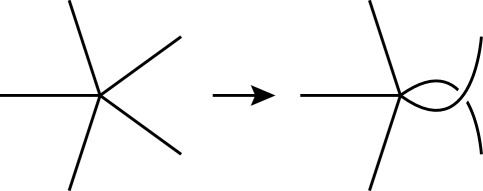
Figure 2.3. A deformation

Next we deform $D^{\prime}$ to $D^{\prime\prime}$ as described below such that there are no crossings of $D^{\prime\prime}$ on $T$. We shrink the edges of $T$ toward $v$. In the process the number of crossings may increase as illustrated in Figure 2.4. In Figure 2.4 only one case of over/under crossing information is illustrated. Another case is similar. To estimate the increase of the number of crossings, we define the following. Let $e$ be an edge of $T$. We denote the shortest path of $T$ containing $e$ and $v$ by $P_{T}(e,v)$. We define a positive integer $b(e)$ for each edge $e$ of $G$ as follows. Set $b(e)=1$ for $e\in E(G)\setminus E(T)$. Let $e$ be an edge of $T$. Let $u$ be a terminal vertex of $P_{T}(e,v)$ with $u\neq v$. Then $u$ is incident to $e$. Suppose that $b(d)$ is already defined for all edges but $e$ incident to $u$. Then $b(e)$ is defined to be the sum of these $b(d)$s where a loop is counted twice. This recursively defines $b(e)$ for all $e\in E(G)$. See for example Figure 2.5. We see from Figure 2.4 that a crossing in $D^{\prime}$ between edges $d$ and $e$ corresponds $b(d)b(e)$ crossings in $D^{\prime\prime}$. Let $a=({\rm max}\{b(e)|e\in E(G)\})^{2}$. Then we have $c(D^{\prime\prime})\leq a\cdot c(D^{\prime})$. Since $c(D^{\prime})\leq c(D)+b$ we have $c(D^{\prime\prime})\leq a\cdot c(D)+ab$. Note that $D^{\prime\prime}$ cannot be a knotted projection. In fact a descending algorithm under any ordering and orientation of the edges $E(G)\setminus E(T)$ produce a trivial embedding of $G$. Therefore we have $\displaystyle{u(f)\leq\frac{1}{2}c(D^{\prime\prime})}$. Thus we have $\displaystyle{u(f)\leq\frac{1}{2}(a\cdot c(D)+ab)}$. Set $\displaystyle{A=\frac{1}{2}a}$ and $\displaystyle{B=\frac{1}{2}ab}$ we have $\displaystyle{u(f)\leq A\cdot c(f)+B}$. $\Box$

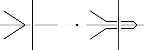
Figure 2.4. A deformation

Figure 2.5. An example

References

[1]D. Buck and D. O’Donnol, Unknotting numbers for prime -curves up to seven crossings, preprint. (arXiv:1710.05237)
[2]W. Mason, Homeomorphic continuous curves in -space are isotopic in -space, Trans. Amer. Math. Soc., 142 (1969), 269-290.
[3]R. Nikkuni, M. Ozawa, K. Taniyama and Y. Tsutsumi, Newly found forbidden graphs for trivializability, J. Knot Theory Ramifications, 14 (2005), 523-538.
[4]I. Sugiura and S. Suzuki, On a class of trivializable graphs, Sci. Math., 3 (2000), 193-200.
[5]N. Tamura, On an extension of trivializable graphs, J. Knot Theory Ramifications, 13 (2004), 211-218.
[6]K. Taniyama, Knotted projections of planar graphs, Proc. Amer. Math. Soc., 123 (1995), 3575-3579.
[7]K. Taniyama, Unknotting numbers of diagrams of a given nontrivial knot are unbounded, J. Knot Theory Ramifications, 18 (2009), 1049-1063.