End to End Binarized Neural Networks for Text Classification

Abstract

Deep neural networks have demonstrated their superior performance in almost every Natural Language Processing task, however, their increasing complexity raises concerns. In particular, these networks require high expenses on computational hardware and training budget is a concern for many. Even for a trained network, the inference phase can be too demanding for resource-constrained devices, thus limiting its applicability. The state-of-the-art transformer models are a vivid example. Simplifying the computations performed by a network is one way of relaxing the complexity requirements. In this paper, we propose an end to end binarized neural network architecture for the intent classification task. In order to fully utilize the potential of end to end binarization, both input representations (vector embeddings of tokens statistics) and the classifier are binarized. We demonstrate the efficiency of such architecture on the intent classification of short texts over three datasets and for text classification with a larger dataset. The proposed architecture achieves comparable to the state-of-the-art results on standard intent classification datasets while utilizing $\sim$ $20$-$40$% lesser memory and training time. Furthermore, the individual components of the architecture, such as binarized vector embeddings of documents or binarized classifiers, can be used separately with not necessarily fully binary architectures.

1 Introduction

In recent years, deep neural networks have achieved great success in a variety of domains including but not limited to autonomous driving [Grigorescu et al., 2020], image recognition [Krizhevsky et al., 2012], and text classification [Kim, 2014]. However, deep networks are becoming more and more computationally expensive due to the ever-growing size of the models being trained. This tendency has been noticed in [Strubell et al., 2019] and it has been recommended that academia and industry researchers should draw their attention towards more computationally efficient methods. At the same time, many important application areas such as chatbots, IoT devices, mobile devices and other types of power-constrained and resource-constrained platforms require solutions that would be highly computation and memory efficient. Such use-cases limit the potential use of the state-of-the-art deep networks. One viable solution is the transformation of these high-performance neural networks to a more computationally efficient architecture. For example, continuous values of the network’s parameters (e.g., float $32$-$64$ bits) can be quantized into discrete integer values. Recently, Binarized Convolutional Neural Networks (BNN) [Hubara et al., 2016] have been developed where both weights and activations are restricted to $\{+1,-1\}$. This results in highly computationally efficient networks with a much lower memory footprint. However, to the best of our knowledge, in the area of text classification in general and intent classification, in particular, no end to end trainable binarized architecture has been demonstrated yet.

In this paper, we introduce an architecture for the task of intent classification that fully utilizes the power of binary representations. The input representations are tokenized and embedded in binary high-dimensional (HD) vectors forming distributed representations using the approach known as hyperdimensional computing [Kanerva, 2009], [Rachkovskij, 2001]. The binary input representations are used for training an end to end BNN classifier for intent classification. Classification performance-wise, the binarized architecture achieves the results comparable to the state-of-the-art on three standard intent classification datasets [Braun et al., 2017] but performs less accurately on a large text classification 20NewsGroups [Lang, 1995] dataset. The efficiency of the proposed architecture is shown in terms of its time and memory complexity relative to non-binarized architectures. For example, it reduces the memory consumption by about $40$% when compared to a non-binarized neural network using GloVe embeddings [Pennington et al., 2014] as the input representation.

Thus, the main contributions of this paper are as follows:

• We introduce a fully end to end binarized architecture for the task of intent classification that uses binary representations followed by the binarized classifier.

• We show that the proposed architecture preserves classification performance while being more time and memory-efficient compared to the non-binarized architecture.

• Finally, we show that the components of the architecture can be used individually as parts of solutions for other NLP tasks.

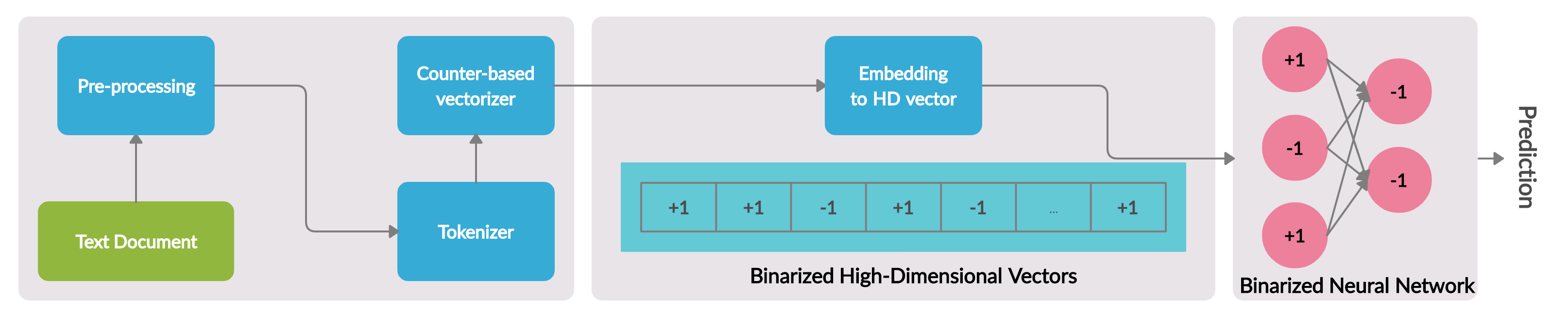
Figure 1: A schematic diagram of the end to end binarized classification architecture for text classification

2 Related Work

2.1 Tokenization

Classical methods such as word-based tokenizers were one of the most popular tokenization methods to form a dictionary. They, however, suffer from out-of-dictionary problems for unseen words [Bojanowski et al., 2017]. $n$-gram based tokenization estimates the out-of-dictionary words better. They can also be used to represent words [Joulin et al., 2016]. As an alternative to word/token representation [Shridhar et al., 2019] introduced the idea of Subword Semantic Hashing that marks the start and end of a word with a specialized token and defines a hashing function to form $n$-gram-based subword tokens. Byte-Pair-Encoding (BPE) [Sennrich et al., 2015] is another popular subword segmentation method widely used in many neural machine translation systems. The main idea of the BPE is to split the sentence into individual tokens and to merge the most frequent tokens to get the final representation. The area was further extended by  [Kudo, 2018] using a unigram language model. Most recently, a highly successful Bidirectional Encoder Representations from Transformers (BERT) model [Devlin et al., 2018] has proven to be a good tokenization choice where the tokenization is based on BERT’s masking objective.

2.2 Representation of tokens

Conventional $n$-gram statistics uses sparse localist representations. In the special case, when $n=1$, it can be seen as count-based vectors and compatible with Term Frequency Inverse Document Frequency (TF-IDF). Note that these representations are proportional to the length of the tokens’ dictionary. Moreover, the length of representations grows exponentially with $n$, making them highly inefficient in terms of memory. Hyperdimensional computing-based embedding of $n$-gram statistics [Joshi et al., 2016], [Alonso et al., 2020] is used to represent the tokens extracted from the input text into a vector of fixed size, which does not depend on $n$. Previous works have shown the usefulness of these embeddings for the tasks of language identification [Rahimi et al., 2016], [Kleyko et al., 2019] and news articles classification [Najafabadi et al., 2016]. This work differs from the ones mentioned above, as in these studies, the embeddings were not combined with a trainable architecture. In contrast, here, the binary embeddings are used as a part of the architecture representing the input text, which enters a BNN.

As an alternative to $n$-gram based representations, dense trainable word embeddings (e.g., word2vec [Mikolov et al., 2013] or GloVe [Pennington et al., 2014]) use a fixed size vector representation. These embeddings are based on the distributional hypothesis and are expected to represent words with similar meanings nearby in the embedding space. However, the drawbacks of such embeddings are that they require pre-training on large text corpora and that storage of the trained embeddings demands a non-negligible memory footprint.

2.3 Classification models

In recent years, convolutional neural networks have been shown to be useful for NLP classification tasks at the level of sentences [Kim, 2014] when trained on top of the pre-trained word embeddings. Moreover, token-level convolutional networks [Zhang et al., 2015] have achieved state-of-the-art or competitive results on several large scale classification datasets. BNNs [Hubara et al., 2016], on the other hand, have been extensively used for computer vision tasks and their application to NLP tasks has been limited. One such example is [Zheng and Tang, 2016], where the binarized recurrent neural network has been used for the language modeling task. In this work, we show that BNNs are applicable for intent classification. We further show that the binarization capabilities are enhanced when using a fully binarized architecture, including embeddings and classifiers.

3 Methods

This section introduces a variety of methods used in the experiments. Figure 1 presents a schematic overview of the architecture. Given an input text document $D$, we first pre-process the document (see Section 4.2 for more details). The pre-processed document is then tokenized into the corresponding tokens $<T_{1},T_{2},...,T_{n}>$ using one of the methods below. The tokens are used as an input to a count-based vectorizer. The representation of vectorizers, which is sparse and localist, is embedded into an HD vector (distributed representation) using hyperdimensional computing [Rahimi et al., 2017]. Hyperdimensional computing is tightly related to randomly connected neural networks [Kleyko et al., 2020], [Kleyko et al., 2017] but it allows constructing more complex representations such as data structures [Osipov et al., 2017]. Moreover, HD vector representing the counter’s content can be binarized. It is used as an input to a classifier. The main classifier studied in this work is BNN but other classifiers are also considered for benchmarking.

3.1 Tokenizers

3.1.1 Word tokenizer

Given a pre-processed text $D$, a word tokenizer splits the input text $D$ into tokes $<T_{1},T_{2},...,T_{n}>$ corresponding to words. Words are split based on spaces while throwing away certain tokens, such as punctuation marks, unidentified tokens, hyphen symbols and others. For a sample text sentence $D$, [“hello! how are you?”], its word tokens would be [“hello”, “how”, “are”, “you”].

3.1.2 Semantic Hashing tokenizer

First, Subword Semantic Hashing (SemHash) splits the input text $D$ into word tokens $<T_{1},T_{2},...,T_{n}>$. Next, for each word token $T_{i}$, SemHash creates subword tokens using a hashing method. For a given pre-processed input sample text $D$, e.g., [“hello how are you”], the output of the word split-step would be: [“hello”, “how”, “are”, “you”]. A hashing function $\mathcal{H}(T_{i})$ adds $\#$ at the beginning and end of each word token. Subwords are extracted for every token as $n$-grams for a given value of $n$, for example, when $n=3$, $\mathcal{H}(hello)$=[“#he”, “hel”, “ell”, “llo”, “lo#”].

3.1.3 Byte Pair Encoding tokenizer

Given as input a pre-processed text $D$, BPE [Sennrich et al., 2015] splits the sentences into individual words with special end of word token $\dot{g}$ and merges the most frequent tokens to get the final tokens. This is highly efficient for representing the unknown words into known frequent token sets. For a given input sample text $D$, e.g., [“hello how are you”], the output of the BPE tokenizer would be: [“hello$\dot{g}$”, “how$\dot{g}$”, “are$\dot{g}$”, “you”].

3.1.4 Char level Byte Pair Encoding tokenizer

For better subword sampling, [Kudo, 2018] proposed a new subword segmentation method based on a unigram language model. The unigram language model is based on an independent subword occurrence assumption with the probability of a subword sequence defined as the product of the subword occurrence probabilities. For a given input sample text $D$, e.g., [“hello how are you”], the output of the Char level BPE tokenizer would be: [“h”, “e”, “l”, “l”, “o$\dot{g}$”, “h”, “o”, “w$\dot{g}$”, “a”, “r”, “e$\dot{g}$”, “y”, “o”, “u$\dot{g}$”] where $\dot{g}$ is the special token to mark the end of the word.

3.1.5 BERT-based tokenizer

The BERT-based tokenizer is based on the BERT architecture, as proposed by [Devlin et al., 2018]. It learns the token splits based on the masking objective on an unsupervised dataset. For a given input sample text $D$, e.g., [“hello how are you”], the output of the BERT-based tokenizer would be: [“[cls]”, “hello”, “how”, “are”, “you”, “[sep]”] where “[cls]” is the special token used to mark the start of the sentence and “[sep]” is the sentence separator.

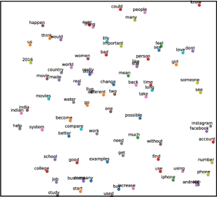
(a) t-SNE projection with GloVe embeddings

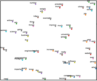
(b) t-SNE projection with HD embeddings

Figure 2: (a) shows the t-SNE projection with GloVe embeddings, while (b) shows the t-SNE projection with HD vectors; GloVe is pre-trained on the Quora question pairs datasetwhile HD vectors are directly obtained from $n$-gram statistics of the words present in the plot. Colours of points are not associated to any meaning.

3.2 High-Dimensional embedding of vectorized representations

The vectorized representations containing the statistics of tokens extracted from the pre-processed documents are usually sparse and have high dimensionality. In order to reduce the dimensionality of representations, we use hyperdimensional computing [Frady et al., 2020]. First, each unique token $T_{i}$ is assigned with a random $d$-dimensional bipolar HD vector, where $d$ would be a hyperparameter of the method. HD vectors are stored in the item memory, which is a matrix $\textbf{H}\in[d\times n]$. Thus, for a token $T_{i}$ there is an HD vector $\textbf{H}_{T_{i}}\in\{-1,+1\}^{[d\times 1]}$. To construct composite representations from the basic HD vectors stored in H, hyperdimensional computing defines three key operations: permutation ($\rho$), binding ($\odot$, implemented via position-wise multiplication), and bundling ($+$, implemented via position-wise addition). For detailed properties and definitions of hyperdimensional computing operations, please see [Kanerva, 2009]. The bundling operation allows storing information in HD vectors [Frady et al., 2018]. Three operations above allow embedding vectorized representations based on $n$-gram statistics into an HD vector [Joshi et al., 2016]. Note that a vectorizer that simply counts the number of times each token is present in the document is the special case of $n$-gram statistics for $n=1$.

We first generate H, which has an HD vector for each token. The permutation operation $\rho$ is applied to $\textbf{H}_{T_{j}}$ $j$ times ($\rho^{j}(\textbf{H}_{T_{j}})$) to represent a relative position of token $T_{j}$ in an $n$-gram. A single HD vector corresponding to an $n$-gram (denoted as m) is formed using the consecutive binding of permuted HD vectors $\rho^{j}(\textbf{H}_{T_{j}})$ representing tokens in each position $j$ of the $n$-gram. For example, the trigram ‘#he’ will be embedded to an HD vector as follows: $\rho^{1}(\textbf{H}_{\text{\#}})\odot\rho^{2}(\textbf{H}_{\text{h}})\odot\rho^{3}(\textbf{H}_{\text{e}})$. In general, the process of forming HD vector of an $n$-gram is formalized as follows:

$$\textbf{m}=\prod_{j=1}^{n}\rho^{j}(H_{T_{j}}),$$

where $T_{j}$ is token in $j$th position of the $n$-gram; the consecutive binding operations applied to $n$ HD vectors are denoted by $\prod$. Once it is known how to form an HD vector for an individual $n$-gram, embedding the $n$-gram statistics into an HD vector h is achieved by bundling together all $n$-grams observed in the document:

$$\textbf{h}=[\sum_{i=1}^{k}f_{i}\textbf{m}_{i}=\sum_{i=1}^{k}f_{i}\prod_{j=1}^{n}\rho^{j}(H_{T_{j}})],$$

where $k$ is the total number of $n$-grams; $f_{i}$ is the frequency of $i$th $n$-gram and $\textbf{m}_{i}$ is the HD vector of $i$th $n$-gram; $\sum$ denotes the bundling operation when applied to several HD vectors; $[*]$ denotes the binarization operation, which is implemented via the sign function. The usage of $[*]$ is optional, so we can either obtain binarized or non-binarized h. If h is non-binarized, its components will be integers in the range $[-k,k]$ but these extreme values are highly unlikely since HD vectors for different $n$-grams are quasi-orthogonal, which means that in the simplest (but not practical) case when all $n$-grams have the same probability the expected value of a component in h is $0$. Due to the use of $\sum$ for representing $n$-gram statistics, two HD vectors embedding two different $n$-gram statistics might have very different amplitudes if the frequencies in these statistics are very different. When HD vectors h are binarized, this issue is addressed. In the case of non-binarized HD vectors, we address it by using the cosine similarity, which is imposed by normalizing each h by its $\ell_{2}$ norm, thus, all h have the same norm and their dot product is equivalent to their cosine similarity. Figure 2 provides an example of t-SNE projections of words represented either as GloVe embeddings or as embedding of $n$-gram statistics to HD vectors.

3.3 Binarized Neural Networks

Based on the work of [Hubara et al., 2016], we construct BNNs capable of working with representations of texts. To take the full advantage of binarized HD vectors, we constraint the weights and activations of the network layers to be $\{+1,-1\}$. This constraint is highly efficient in terms of hardware and memory, as bit-wise operations are used instead of multiply-accumulate operations. For example, a multiplication on binary values can be performed using an XNOR logical operation.

The vectorized representations of tokens embedded into HD vectors are binarized with all values $\{+1,-1\}$. In the case of HD vectors, we binarize the result of the bundling operation using the ${\rm sign}$ function. Similarly, the ${\rm sign}$ function is used in the BNN for every weight or activation to restrict them into $\{+1,-1\}$ as follows:

$$b(x)=[x]={\rm sign}(x)=\left\{\begin{array}[]{ll}+1&\mbox{if $x\geq 0$},\\ -1&\mbox{otherwise}\end{array}\right.$$ (1)

where, $x$ can be any weight or activation value.

We further define a convolutional 1D layer that creates a convolution kernel that is convolved with the input HD vector over a single spatial dimension to produce a tensor of outputs. Since gradient descent methods make small changes to the value of the weights, which cannot be done with binary values, we use the straight-through estimator (STE) idea, as mentioned in [Yin et al., 2019]. We also define a value over which we clip the gradients in the backward pass:

$$\frac{\delta b(x)}{\delta x}=\left\{\begin{array}[]{ll}+1&\mbox{if $|x|<\text{clip value}$},\\ 0&\mbox{otherwise}\end{array}\right.$$ (2)

This ensures that the entire architecture is end to end trainable using the gradient descent optimization.

4 Empirical Analysis

4.1 Datasets

All the experiments in this paper are performed on four datasets, namely: the Chatbot Corpus (Chatbot), the Ask Ubuntu Corpus (AskUbuntu), the Web Applications Corpus (WebApplication), and the 20 News Groups Corpus (20NewsGroups). The Chatbot, AskUbuntu and WebApplication datasets are used for short text intent classification and were taken from [Braun et al., 2017]. The datasets are available on GitHub; 20NewsGroups dataset is available within the sklearn [Buitinck et al., 2013] library.

Chatbot Corpus:

The Chatbot Corpus was collected from questions posted using a Telegram Chatbot. The classification task was performed on $2$ intents: (Departure Time and Find Connection) with $206$ questions. The train set consists of $100$ samples, while $106$ samples were used as the test set.

AskUbuntu Corpus:

The AskUbuntu Corpus has been extracted from the AskUbuntu platform. It consists of $5$ intents (Make Update, Setup Printer, Shutdown Computer, Software Recommendation, and None) with $53$ training samples and $109$ test samples.

WebApplication Corpus:

The WebApplication Corpus consists of $88$ samples and $8$ intents (Change Password, Delete Account, Download Video, Export Data, Filter Spam, Find Alternative, Sync Accounts, and None) with $30$ training samples and $58$ test samples.

20NewsGroups Corpus:

The 20NewsGroups consists of news post categorized into $20$ categories. Each category has exactly $18846$ text samples with $11314$ samples for training and $7532$ samples for testing. A detailed data distribution for each dataset is provided in the Appendix.

	Chatbot		AskUbuntu		WebApplication		20NewsGroups
Tokenizers	Text-LeNet	BNN	Text-LeNet	BNN	Text-LeNet	BNN	Text-LeNet	BNN
Word	0.80	0.73	0.51	0.79	0.56	0.78	0.54	0.56
SemHash	0.94	0.90	0.87	0.84	0.79	0.83	0.78	0.69
BPE	0.80	0.58	0.54	0.67	0.52	0.75	0.38	0.42
Char BPE	0.92	0.81	0.76	0.76	0.55	0.53	0.55	0.48
SentencePiece	0.80	0.99	0.70	0.72	0.50	0.70	0.41	0.43
BERT	0.89	0.88	0.72	0.71	0.70	0.77	0.60	0.60

Table 1: $F_{1}$ performance comparison of binarized Text-LeNet (BNN) architecture with non-binarized Text-LeNet for the task of intent classification on various datasets.

Datasets	Binarized GloVe	Binarized SemHash	Binarized HD vectors
Chatbot	0.74	0.91	0.99
AskUbuntu	0.86	0.87	0.84
WebApplication	0.66	0.80	0.83
20NewsGroups	0.62	0.64	0.69

Table 2: $F_{1}$ performance comparison of Binarized GloVe vectors, Binarized SemHash vectors and Binarized HD vectors. All vectorizers use the same binarized Text-LeNet architecture as classifier.

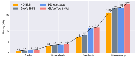
(a) Memory Comparison

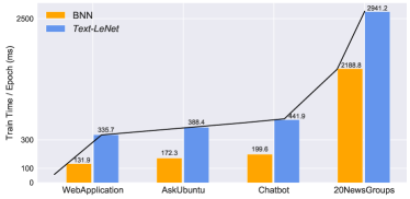
(b) Train Time per epoch Comparison

Figure 3: (a) shows the memory comparisons for all 4 datasets using HD Text-LeNet, HD BNN, GloVe Text-LeNet, GloVe BNN and (b) shows the training time per epoch comparison for all 4 datasets using BNN and Text-LeNet

4.2 Experimental Details

On all datasets, six tokenization methods were used, namely: Word-based, SemHash, BPE, Char level BPE, Sentence Piece and BERT-based. For Word-based tokenizer, the datasets were pre-processed using the Spacy library to remove stop words from data. Spacy pre-trained model “en_core_web_lg” was used to parse the datasets. All text samples were also pre-processed by removing control tokens, in particular, the ones in the set [Cc], which includes Unicode tokens from U+0000 to U+009F. The small datasets (Chatbot, WebApplication and AskUbuntu) data samples within each class were made equal to the largest class sample size by augmenting the data. For SemHash, $n$ value was kept at $3$, and all trigrams were considered. For BPE, a dictionary size of $1000$ was used for Chatbot, WebApplication and AskUbuntu, and $2000$ for 20NewsCorpus dataset because of its larger size. Similar values were used for Char-based BPE and Sentence Piece tokenizers. The difference between Sentence Piece and BPE is that Sentence Piece uses stop words removal before tokenization while BPE and Char-based BPE do not. BERT-based tokenizer was pre-trained on a large corpus “bert-large-cased-vocab.txt” that contains $29213$ unique words and has been provided by the Huggingface library.

For the purpose of benchmarking, nine sklearn classifiers were applied to the intent classification datasets: MLP, Random Forest, Linear SVC, Passive Aggressive, SGD Classifier, Ridge Classifier, Nearest Centroid, Bernoulli NB, KNN Classifier with an HD vector size of $d=\{512,1024,4098,8192,16384\}$. The detailed results for these classifiers are provided in the Appendix. CNN-based architecture used $d=\{512,1024,4098,8192\}$ as embedding sizes. 20NewsGroups dataset was run with MLP, Random Forest, Linear SVC and SGD classifiers for embedding sizes $d=\{512,1024,4096,16384\}$ and with CNN for sizes $d=\{512,1024,4096\}$.

For CNN-based architecture, $5$ hidden layers were used: $3$ convolutional $1$D layers followed by $2$ dense layers. Due to its resemblance to the original LeNet architecture [LeCun et al., 1998], we refer to this architecture as to Text-LeNet. The detailed configuration is provided in the Appendix. We noted in the experiments that Batch Normalization [Ioffe and Szegedy, 2015] is very helpful for faster convergence of the network and, therefore, it was added after every convolutional and dense layer. The clip value for the gradients was set to $1$ during the backward pass. RMSProp [Hinton et al., 2012] was used as the optimizer with a learning rate of $1$e-$3$ and categorical cross-entropy as the loss function. All the checkpoints were saved in the h5 format. Larq Compute Engine [Geiger and Team, 2020], a highly optimised engine for quantization of networks, was used to convert the h5 files to tflite format for BNNs.

For classifiers, that were a part of the grid-based search, the paper reports the results for the best hyperparameters. For all other classifiers the default hyperparameter settings provided by the sklearn library were used. A $5$-fold cross-validation was used in the experiments. A total of $5$ simulations were performed and the average results are reported in the paper. All sklearn-based classifier experiments were performed on the CPU and CNN-based experiments were performed on NVIDIA Tesla GPUs.

4.3 Results and Discussions

To demonstrate the efficiency of binarized architecture for the intent classification task, we compare the results of binarized HD vectors with the binarized Text-LeNet (BNN) architecture as classifier against non-binarized HD vectors with non-binarized Text-LeNet. The $F_{1}$ scores are compared in Table 1 where BNN performed equally well to a Text-LeNet architecture while being $20$% to $40$% more memory efficient, as shown in Figure 3(a). Due to the specifics of implementation, BNNs use $32$ bit float values as Text-LeNet. The memory efficiency of BNNs can be further improved by $4$x when $8$-bit representations are used. On performance side, BNNs outperforms the Text-LeNet for AskUbuntu and WebApplication datasets on $4$ out of $6$ tokenizers. The results reported in Table 1 used $512$ dimensional HD vectors for Chatbot, AskUbuntu and WebApplication corpus, while $1024$ dimensional HD vectors were used for 20NewsGroups dataset. The choice of dimensionality was based on the size of the datasets and a larger dimensionality was used for larger datasets.

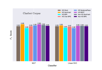
(a) Chatbot Corpus

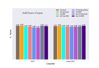
(b) AskUbuntu Corpus

(c) WebApplication Corpus

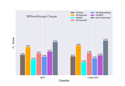
(d) 20NewsGroups Corpus

Figure 4: (a), (b), (c) and (d) shows the $F_{1}$ score comparison of MLP and Linear SVC classifier with HD and non-HD based tokenizers on Chatbot, AskUbuntu, WebApplication and 20NewsGroups corpus respectively.

One thing to note here is that Text-LeNet also used HD vectors with the mentioned tokenizers, but the HD vectors were non-binarized. HD vectors in itself are already faster and much more efficient than counter-based representations, as shown in [Alonso et al., 2020]. When experimenting with other embedding methods like GloVe, the training was significantly slower; therefore, HD vectors were used for all the experiments. In addition to that, using binarized classifier (BNN) further improves the training time upto $50\%$ compared to non-binarized classifier on all four datasets as shown in Figure  3 (b). Furthermore, when compared to GloVe embeddings with Text-LeNet, HD BNN used around $20$ - $40$% lesser memory for all the intent classification datasets.

To justify that the binarization of HD vectors is effective and needed in this work, we benchmarked the binarized HD vectors with binarized $300$-dimensional GloVe vectors and the binarized version of counter-based representation for SemHash tokenizer for all the datasets. Table 2 summarizes the results of the comparison. All the binarized representations were trained with the same BNN classifier. Binarized HD vectors performed significantly better than other binarized methods outperforming binarized GloVe by $4$ - $25$% and binarized SemHash by $2$ - $8$% on $2$ out of $3$ smaller intent classification datasets and achieves comparable results for AskUbuntu dataset. The trend continued for 20NewsGroups with binarized HD achieving $5$ - $7$% better $F_{1}$ scores. Note that for the SemHash counter-based vectorizer, we put a sign function $sign(x)=+1\ \text{for}\ x>0\ \text{and}\ -1\ \text{otherwise}$.

In Figure 4, MLP and Linear SVC with all the tokenizers with HD vectors as representation are compared with MLP and Linear SVC classifiers with SemHash tokenizers and counter-based vectorizer as representation from [Alonso et al., 2020]. The $F_{1}$ score is comparable to the state-of-the-art for both MLP and SVC. For all small intent classification datasets, binarized HD vectors have achieved better results than non-HD vectors. The proposed architecture beats the non-HD baselines by $+2$% for AskUbuntu and Chatbot Corpus, and $+5$% for WebApplication Corpus. However, for 20NewsGroups the results of binarized HD Vectors are lower than non-HD Vectors. This is mainly due to the large size of the dataset and simple classifiers like LinearSVC failed to perform with just binarized values. The results for all the other classifiers are provided in the Appendix.

Table 3 compares the $F_{1}$ scores of various platforms on the intent classification datasets. We report the results of binarized HD vectors with the best classifiers from one of the nine classifiers mentioned (Binarized HD vectors with the best classifier), non-binarized HD vectors with Text-LeNet (HD Text-LeNet) and binarized HD vectors with binarized Text-LeNet (HD BNN). Our end to end binarized architecture (HD BNN) achieved the state-of-the-art results for Chatbot dataset. The approach where only HD vectors were binarized (binarized HD vectors with the best classifier) achieved the state-of-the-art results for AskUbuntu dataset. The results on WebApplication dataset are comparable to the state-of-the-art ($0.87$ with SemHash): $0.84$ for binarized HD vectors with the best classifier and $0.83$ for HD BNN. The average performance of both binarized HD vectors with the best classifier ($0.92$) and HD BNN ($0.91$) was also comparable to the best non-binarized approach ($0.92$ with Semhash).

Platform	Chatbot	AskUbuntu	WebApplication	Average
Botfuel	0.98	0.90	0.80	0.89
Luis	0.98	0.90	0.81	0.90
Dialogflow	0.93	0.85	0.80	0.86
Watson	0.97	0.92	0.83	0.91
Rasa	0.98	0.86	0.74	0.86
Snips	0.96	0.83	0.78	0.86
Recast	0.99	0.86	0.75	0.87
TildeCNN	0.99	0.92	0.81	0.91
FastText	0.97	0.91	0.76	0.88
SemHash	0.96	0.92	0.87	0.92
BPE	0.95	0.93	0.85	0.91
HD vectors  [Alonso et al., 2020]	0.97	0.92	0.82	0.90
Binarized HD vectors with the best classifier	0.98	0.93	0.84	0.92
HD Text-LeNet	0.94	0.87	0.79	0.88
HD BNN	0.99	0.84	0.83	0.91

Table 3: $F_{1}$ score comparison of various platforms on intent classification datasets of short texts with methods used in the paper. Some results are taken from [Alonso et al., 2020]

5 Conclusion

In this work, we present an end to end binarized architecture for the intent classification task. We demonstrate that it is possible to achieve comparable to the state-of-the-art results while using the binarized representations of all the components of the NLP classification architecture. This allows exploring the effectiveness of binary representations both for reducing the memory footprint of the architecture and for increasing the energy-efficiency of the inference phase due to effectiveness of binary operations. This work takes a step towards enabling NLP functionality on resource-constrained devices.

Appendix A Appendix

A.1 Datasets

The experiments in the paper were performed on four datasets: the Chatbot Corpus (Chatbot), the Ask Ubuntu Corpus (AskUbuntu), the Web Applications Corpus (WebApplication), and the 20 News Groups Corpus (20NewsGroups).

A chatbot was created on Telegram, where questions of the public transport of Munich were posted. The chatbot replied to the questions and thus data was collected for the Chatbot corpus. A detailed test and train split are provided in Table 1.

Intent	Train original	Train Augmented	Test
Departure Time	43	57	35
Find Connection	57	57	71

Table 1: Data sample distribution for the Chatbot dataset

The AskUbuntu and WebApplication datasets are questions and answers from the StackExchange platform. A detailed breakdown is provided in Table 2 and 3 respectively.

Intent	Train original	Train Augmented	Test
Make Update	10	17	37
Setup Printer	10	17	13
Shutdown Computer	13	17	14
Software Recommendation	17	17	40
None	3	17	5

Table 2: Data sample distribution for the AskUbuntu dataset

Intent	Train original	Train Augmented	Test
Change Password	2	7	6
Delete Account	7	7	10
Download Video	1	7	0
Export Data	2	7	3
Filter Spam	6	7	14
Find Alternative	7	7	16
Sync Accounts	3	7	6
None	2	7	4

Table 3: Data sample distribution for the WebApplication dataset

The 20NewsGroups dataset comprises news posts labelled into several categories and a detailed breakdown is provided in Table 4.

Categories	Train	Test
alt.atheism	11314	7532
comp.graphics	11314	7532
comp.os.ms-windows.misc	11314	7532
comp.sys.ibm.pc.hardware	11314	7532
comp.sys.mac.hardware	11314	7532
comp.windows.x	11314	7532
misc.forsale	11314	7532
rec.autos	11314	7532
rec.motorcycles	11314	7532
rec.sport.baseball	11314	7532
rec.sport.hockey	11314	7532
sci.crypt	11314	7532
sci.electronics	11314	7532
sci.electronics	11314	7532
sci.space	11314	7532
soc.religion.christian	11314	7532
talk.politics.guns	11314	7532
talk.politics.mideast	11314	7532
talk.politics.misc	11314	7532
talk.religion.misc	11314	7532

Table 4: Data sample distribution for the 20NewsGroups dataset

A.2 Experimentation Details

The Text-LeNet architecture used in the experiments is defined as follows:

Text-LeNet

: $[128,M,BN,256,M,BN,512,M,F,128_{D},DO,C]$

where, numbers 128, 256 and 512 represents the filters of Convolution layer which is followed by an activation function. M represents the Max Pooling layer and BN represents the Batch Normalization layer. F refers to a Flatten layer. $128_{D}$ represents the Dense layer of size $128$ followed by a Dropout layer denoted by DO. Finally, C represents the Linear classification layer of dimension ($128$, number of classes).

Other hyper-parameters settings include:

Hyper-parameter	Value
Convolution Kernel Size	$3$
Convolution layer Padding	valid
Max-Pooling Kernel Size	$3$,$2$,$3$ for the three $M$ layers respectively
Optimizer	RMSprop
Loss	Categorical cross entropy
Activation Function	Rectified Linear Unit (ReLU)
Batch Size	$4$ (small datasets) and $64$ (20NewsGroups)
Learning Rate	$0.001$
Number of Epochs	$15$-$40$ (Depending upon the dataset)
Initializer	Xavier initialization

Table 5: Hyper-parameters for the experiments

To find the best hyperparameters, a grid-based search was applied to all the datasets for the MLP classifier. Three different hidden layer configurations were considered: [($100,50$), ($300,100$), ($300,200,100$)]. The best parameters were chosen based on GridSearchCV. The maximal number of iterations for MLP was set to $200$.

In the case of Random Forest, two hyperparameters include optimized number of estimators ([$50,60,70$]) and minimum samples leaf ([$1,11$]); we used $50$ estimators and $1$ leaf. In the case of KNN, the number of neighbors between $3$ and $7$ was considered; $3$ neighbors were used in the experiments. For all the other classifiers the default hyperparameter settings provided by the sklearn library were used.

A.3 Experiments

Table 6-8 compares the $F_{1}$ scores of nine classifiers: MLP, Random Forest, Linear SVC, Passive Aggressive, SGD Classifier, Ridge Classifier, Nearest Centroid, Bernoulli NB, KNN Classifier on all three small datasets with HD versions of six tokenization methods and Non HD versions of SemHash and BPE for small datasets and Non HD SemHash for 20NewsGroups Corpus. SP is an acronym for Sentence Piece. Table 9 compares the results of all the tokenizers using four classifiers: MLP, SGD Classifier, Linear SVC and Random Forest for the 20NewsGroups dataset. SemHash tokenizer, in general, achieved better results compared to other tokenizers followed by BERT tokenizer on all four datasets.

Classifier	HD Word	HD SemHash	HD BPE	HD Char BPE	HD SP	HD BERT	Non HD SemHash	Non HD BPE
MLP	0.92	0.93	0.89	0.90	0.88	0.87	0.92	0.91
Passive Aggr.	0.92	0.93	0.90	0.88	0.91	0.90	0.92	0.93
SGD Classifier	0.86	0.89	0.85	0.88	0.86	0.89	0.89	0.89
Ridge Classifier	0.92	0.92	0.88	0.87	0.91	0.92	0.90	0.91
KNN Classifier	0.81	0.84	0.78	0.60	0.80	0.79	0.79	0.72
Nearest Centroid	0.91	0.91	0.88	0.86	0.86	0.85	0.90	0.89
Linear SVC	0.91	0.92	0.90	0.90	0.89	0.90	0.90	0.92
Random Forest	0.90	0.92	0.82	0.83	0.83	0.82	0.88	0.90
Bernoulli NB	0.76	0.87	0.74	0.84	0.65	0.79	0.91	0.92

Table 6: $F_{1}$ scores of all sklearn classifiers for AskUbuntu dataset.

Classifier	HD Word	HD SemHash	HD BPE	HD Char BPE	HD SP	HD BERT	Non HD SemHash	Non HD BPE
MLP	0.93	0.98	0.88	0.93	0.95	0.98	0.96	0.94
Passive Aggr.	0.96	0.96	0.92	0.94	0.89	0.94	0.95	0.91
SGD Classifier	0.95	0.97	0.93	0.89	0.89	0.92	0.93	0.93
Ridge Classifier	0.94	0.95	0.77	0.91	0.84	0.88	0.94	0.94
KNN Classifier	0.86	0.86	0.80	0.83	0.80	0.91	0.75	0.71
Nearest Centroid	0.79	0.89	0.90	0.86	0.88	0.88	0.89	0.94
Linear SVC	0.93	0.95	0.89	0.92	0.88	0.94	0.94	0.93
Random Forest	0.88	0.91	0.77	0.83	0.85	0.92	0.95	0.95
Bernoulli NB	0.81	0.88	0.81	0.89	0.84	0.91	0.93	0.93

Table 7: $F_{1}$ scores of all sklearn classifiers for Chatbot dataset.

Classifier	HD Word	HD SemHash	HD BPE	HD Char BPE	HD SP	HD BERT	Non HD SemHash	Non HD BPE
MLP	0.82	0.82	0.77	0.78	0.75	0.80	0.77	0.77
Passive Aggr.	0.83	0.83	0.76	0.80	0.80	0.80	0.82	0.80
SGD Classifier	0.76	0.79	0.66	0.64	0.64	0.84	0.75	0.74
Ridge Classifier	0.79	0.84	0.79	0.78	0.76	0.81	0.79	0.80
KNN Classifier	0.80	0.81	0.78	0.67	0.80	0.84	0.72	0.75
Nearest Centroid	0.77	0.80	0.72	0.76	0.75	0.75	0.74	0.73
Linear SVC	0.83	0.85	0.79	0.77	0.80	0.82	0.82	0.80
Random Forest	0.77	0.80	0.61	0.68	0.67	0.78	0.87	0.85
Bernoulli NB	0.61	0.70	0.57	0.62	0.57	0.61	0.74	0.75

Table 8: $F_{1}$ scores of all sklearn classifiers for WebApplication dataset.

Classifier	HD Word	HD SemHash	HD BPE	HD Char BPE	HD SP	HD BERT	Non HD SemHash
MLP	0.44	0.61	0.34	0.47	0.40	0.51	0.72
SGD Classifier	0.43	0.59	0.41	0.26	0.45	0.49	0.70
Linear SVC	0.41	0.64	0.28	0.48	0.37	0.43	0.75
Random Forest	0.17	0.33	0.13	0.20	0.13	0.21	0.58

Table 9: $F_{1}$ scores of sklearn classifiers for 20NewsGroups dataset.

References

- [Alonso et al., 2020] P. Alonso, K. Shridhar, D. Kleyko, E. Osipov, and M. Liwicki. 2020. HyperEmbed: Tradeoffs between Resources and Performance in NLP Tasks with Hyperdimensional Computing Enabled Embedding of n-gram Statistics. arXiv:2003.01821.
- [Bojanowski et al., 2017] P. Bojanowski, E. Grave, A. Joulin, and T. Mikolov. 2017. Enriching word vectors with subword information. Transactions of the Association for Computational Linguistics, 5:135–146.
- [Braun et al., 2017] D. Braun, A. Hernandez-Mendez, F. Matthes, and M. Langen. 2017. Evaluating Natural Language Understanding Services for Conversational Question Answering Systems. In Annual Meeting of the Special Interest Group on Discourse and Dialogue (SIGDIAL), pages 174–185.
- [Buitinck et al., 2013] L. Buitinck, G. Louppe, M. Blondel, F. Pedregosa, A. Mueller, O. Grisel, V. Niculae, P. Prettenhofer, A. Gramfort, J. Grobler, R. Layton, J. VanderPlas, A. Joly, B. Holt, and G. Varoquaux. 2013. API Design for Machine Learning Software: Experiences from the Scikit-learn Project. In ECML PKDD Workshop: Languages for Data Mining and Machine Learning, pages 108–122.
- [Devlin et al., 2018] J. Devlin, M.-W. Chang, K. Lee, and K. Toutanova. 2018. BERT: Pre-training of Deep Bidirectional Transformers for Language Understanding. arXiv:1810.04805.
- [Frady et al., 2018] E. P. Frady, D. Kleyko, and F. T. Sommer. 2018. A Theory of Sequence Indexing and Working Memory in Recurrent Neural Networks. Neural Computation, 30:1449–1513.
- [Frady et al., 2020] E. P. Frady, D. Kleyko, and F. T. Sommer. 2020. Variable Binding for Sparse Distributed Representations: Theory and Applications. arXiv:2009.06734, pages 1–16.
- [Geiger and Team, 2020] L. Geiger and P. Team. 2020. Larq: An Open-Source Library for Training Binarized Neural Networks. Journal of Open Source Software, 5(45):1746, January.
- [Grigorescu et al., 2020] S. Grigorescu, B. Trasnea, T. Cocias, and G. Macesanu. 2020. A Survey of Deep Learning Techniques for Autonomous Driving. Journal of Field Robotics, 37(3):362–386.
- [Hinton et al., 2012] G. Hinton, N. Srivastava, and K. Swersky. 2012. Neural Networks for Machine Learning Lecture 6a Overview of Mini-batch Gradient Descent.
- [Hubara et al., 2016] I. Hubara, M. Courbariaux, D. Soudry, R. El-Yaniv, and Y. Bengio. 2016. Binarized Neural Networks. In Advances in Neural Information Processing Systems (NIPS), pages 1–9.
- [Ioffe and Szegedy, 2015] S. Ioffe and C. Szegedy. 2015. Batch normalization: Accelerating deep network training by reducing internal covariate shift. CoRR, abs/1502.03167.
- [Joshi et al., 2016] A. Joshi, J. T. Halseth, and P. Kanerva. 2016. Language Geometry Using Random Indexing. In Quantum Interaction (QI), pages 265–274.
- [Joulin et al., 2016] A. Joulin, E. Grave, P. Bojanowski, and T. Mikolov. 2016. Bag of Tricks for Efficient Text Classification. arXiv:1607.01759.
- [Kanerva, 2009] P. Kanerva. 2009. Hyperdimensional Computing: An Introduction to Computing in Distributed Representation with High-Dimensional Random Vectors. Cognitive Computation, 1(2):139–159.
- [Kim, 2014] Y. Kim. 2014. Convolutional Neural Networks for Sentence Classification. arXiv:1408.5882.
- [Kleyko et al., 2017] D. Kleyko, E. P. Frady, and E. Osipov. 2017. Integer Echo State Networks: Hyperdimensional Reservoir Computing. arXiv:1706.00280, pages 1–10.
- [Kleyko et al., 2019] D. Kleyko, E. Osipov, D. De Silva, U. Wiklund, V. Vyatkin, and D. Alahakoon. 2019. Distributed Representation of n-gram Statistics for Boosting Self-Organizing Maps with Hyperdimensional Computing. In International Andrei Ershov Memorial Conference on Perspectives of System Informatics (PSI), pages 64–79.
- [Kleyko et al., 2020] D. Kleyko, M. Kheffache, E. P. Frady, U. Wiklund, and E. Osipov. 2020. Density Encoding Enables Resource-Efficient Randomly Connected Neural Networks. IEEE Transactions on Neural Networks and Learning Systems, PP(99):1–7.
- [Krizhevsky et al., 2012] A. Krizhevsky, I. Sutskever, and G. E. Hinton. 2012. Imagenet Classification with Deep Convolutional Neural Networks. In Advances in Neural Information Processing Systems (NIPS), pages 1097–1105.
- [Kudo, 2018] T. Kudo. 2018. Subword Regularization: Improving Neural Network Translation Models with Multiple Subword Candidates. arXiv:1804.10959.
- [Lang, 1995] K. Lang. 1995. Newsweeder: Learning to filter Netnews. In Twelfth International Conference on Machine Learning, pages 331–339.
- [LeCun et al., 1998] Y. LeCun, L. Bottou, Y. Bengio, and P. Haffner. 1998. Gradient-based Learning Applied to Document Recognition. Proceedings of the IEEE, 86(11):2278–2324.
- [Mikolov et al., 2013] T. Mikolov, K. Chen, G. Corrado, and J. Dean. 2013. Efficient Estimation of Word Representations in Vector Space. arXiv:1301.3781.
- [Najafabadi et al., 2016] F. R. Najafabadi, A. Rahimi, P. Kanerva, and J. M. Rabaey. 2016. Hyperdimensional Computing for Text Classification. In Design, Automation and Test in Europe Conference (DATE), pages 1–1.
- [Osipov et al., 2017] E. Osipov, D. Kleyko, and A. Legalov. 2017. Associative Synthesis of Finite State Automata Model of a Controlled Object with Hyperdimensional Computing. In Annual Conference of the IEEE Industrial Electronics Society (IECON), pages 3276–3281.
- [Pennington et al., 2014] J. Pennington, R. Socher, and C. D. Manning. 2014. GloVe: Global Vectors for Word Representation. In Conference on Empirical Methods in Natural Language Processing (EMNLP), volume 14, pages 1532–1543.
- [Rachkovskij, 2001] D. A. Rachkovskij. 2001. Representation and Processing of Structures with Binary Sparse Distributed Codes. IEEE Transactions on Knowledge and Data Engineering, 3(2):261–276.
- [Rahimi et al., 2016] A. Rahimi, P. Kanerva, and J. M. Rabaey. 2016. A Robust and Energy Efficient Classifier Using Brain-Inspired Hyperdimensional Computing. In IEEE/ACM International Symposium on Low Power Electronics and Design (ISLPED), pages 64–69.
- [Rahimi et al., 2017] A. Rahimi, S. Datta, D. Kleyko, E. P. Frady, B. Olshausen, P. Kanerva, and J. M. Rabaey. 2017. High-dimensional Computing as a Nanoscalable Paradigm. IEEE Transactions on Circuits and Systems I, 64(9):2508–2521.
- [Sennrich et al., 2015] R. Sennrich, B. Haddow, and A. Birch. 2015. Neural Machine Translation of Rare Words with Subword Units. arXiv:1508.07909.
- [Shridhar et al., 2019] K. Shridhar, A. Dash, A. Sahu, G. Grund Pihlgren, P. Alonso, V. Pondenkandath, G. Kovacs, F. Simistira, and M. Liwicki. 2019. Subword Semantic Hashing for Intent Classification on Small Datasets. In International Joint Conference on Neural Networks (IJCNN), pages 1–6.
- [Strubell et al., 2019] E. Strubell, A. Ganesh, and A. McCallum. 2019. Energy and Policy Considerations for Deep Learning in NLP. In 57th Annual Meeting of the Association for Computational Linguistics (ACL), pages 3645–3650.
- [Yin et al., 2019] P. Yin, J. Lyu, S. Zhang, S. Osher, Y. Qi, and J. Xin. 2019. Understanding Straight-through Estimator in Training Activation Quantized Neural Nets. arXiv:1903.05662.
- [Zhang et al., 2015] X. Zhang, J. Zhao, and Y. LeCun. 2015. Character-level Convolutional Networks for Text Classification. In Advances in Neural Information Processing Systems (NIPS), pages 649–657. Curran Associates, Inc.
- [Zheng and Tang, 2016] W. Zheng and Y. Tang. 2016. Binarized Neural Networks for Language Modeling. Technical Report cs224d, Stanford University.