Joint Transceiver and Large Intelligent Surface Design for Massive MIMO MmWave Systems

Abstract

Large intelligent surface (LIS) has recently emerged as a potential low-cost solution to reshape the wireless propagation environment for improving the spectral efficiency. In this paper, we consider a downlink millimeter-wave (mmWave) multiple-input-multiple-output (MIMO) system, where an LIS is deployed to assist the downlink data transmission from a base station (BS) to a user equipment (UE). Both the BS and the UE are equipped with a large number of antennas, and a hybrid analog/digital precoding/combining structure is used to reduce the hardware cost and energy consumption. We aim to maximize the spectral efficiency by jointly optimizing the LIS’s reflection coefficients and the hybrid precoder (combiner) at the BS (UE). To tackle this non-convex problem, we reformulate the complex optimization problem into a much more friendly optimization problem by exploiting the inherent structure of the effective (cascade) mmWave channel. A manifold optimization (MO)-based algorithm is then developed. Simulation results show that by carefully devising LIS’s reflection coefficients, our proposed method can help realize a favorable propagation environment with a small channel matrix condition number. Besides, it can achieve a performance comparable to those of state-of-the-art algorithms, while at a much lower computational complexity.

I Introduction

Millimeter-wave (mmWave) communication is regarded as a promising technology for future cellular networks due to its large available bandwidth and the potential to offer gigabits-per-second communication data rates [1, 2, 3, 4]. Utilizing large antenna arrays is essential for mmWave systems as mmWave signals incur a much higher free-space path loss compared to microwave signals below 6 GHz [5, 6]. Large antenna arrays can help form directional beams to compensate for severe path loss incurred by mmWave signals. On the other hand, high directivity makes mmWave communications vulnerable to blockage events, which can be frequent in indoor and dense urban environments. For instance, due to the narrow beamwidth of mmWave signals, a very small obstacle, such as a person’s arm, can effectively block the link [7, 8].

To address this blockage issue, large intelligent surface has been recently introduced to improve the spectral efficiency and coverage of mmWave systems [9, 10, 11, 12]. Large intelligent surface (LIS), also referred to intelligent reflecting surface (IRS), has emerged as a promising technology to realize a smart and programmable wireless propagation environment via software-controlled reflection [13, 14, 15, 16, 17, 18]. Specifically, LIS is a two-dimensional artificial structure, consisting of a large number of low-cost, passive, reconfigurable reflecting elements. With the help of a smart controller, the incident signal can be reflected with reconfigurable phase shifts and amplitudes. By properly adjusting the phase shifts, the LIS-assisted communications system can achieve desired properties, such as extending signal coverage [19], improving energy efficiency[20], mitigating interference [21, 22], enhancing system security [23], and so on.

A key problem of interest in LIS-assisted communication systems is to jointly devise the reflection coefficients at the LIS and the active precoding matrix at the BS to optimize the system performance. A plethora of studies have been conducted to investigate the problem under different system setups and assumptions, e.g. [19, 20, 21, 9, 22, 23, 24, 25, 11, 26, 27, 28]. Among them, most focused on single-input-single-output (SISO) or multiple-input-single-output (MISO) systems [19, 20, 21, 9, 22, 23]. For the MIMO scenario where both the BS and the UE are equipped with multiple antennas, [24] proposed to optimize the spectral efficiency via maximizing the Frobenius-norm of the effective channel from the BS to the UE. Nevertheless, maximizing the Frobenius-norm of the effective channel usually results in a large condition number, and as a result, its performance improvement is limited. In [25], an alternating optimization (AO)-based method was developed to maximize the capacity of LIS-aided point-to-point MIMO systems via jointly optimizing LIS’s reflection coefficients and the MIMO transmit covariance matrix. Specifically, the AO-based method sequentially and iteratively optimizes one reflection coefficient at a time by fixing the other reflection coefficients. Although achieving superior performance, this sequential optimization incurs an excessively high computational complexity for practical systems. In [11], two optimization schemes were proposed to enhance the channel capacity for LIS-assisted mmWave MIMO systems. Nevertheless, this work is confined to the scenario where only a single data stream is transmitted from the BS to the UE. To improve the bit error rate (BER) performance, [26] proposed a geometric mean decomposition (GMD)-based beamforming scheme for LIS-assisted mmWave MIMO systems. To simplify the problem, only the angle of arrival (AoA) of the line-of-sight (LOS) BS-LIS link and the angle of departure (AoD) of the LOS LIS-UE path were utilized to design the reflection coefficients. This simplification, however, comes at the cost of sacrificing the spectral efficiency. Besides the above works, other studies [27, 28] considered multiple-user (MU)-MIMO scenarios. For example, [27] considered using the LIS at the cell boundary to assist downlink transmission to cell-edge users.

In this paper, we consider a point-to-point LIS-assisted mmWave systems with large-scale antenna arrays at the transmitter and receiver, where an LIS is deployed to assist the downlink transmission from the transmitter (i.e. BS) to the receiver (i.e. UE). Our objective is to maximize the spectral efficiency of the LIS-assisted mmWave system by jointly optimizing the LIS reflection coefficients and the hybrid precoding/combining matrices associated with the BS and the UE. To address this non-convex optimization problem, we first decouple the LIS design from hybrid precoder/combiner design. We then focus on the reflection coefficient optimization problem. By exploiting the inherent structure of the effective mmWave channel, it is shown that this complex LIS optimization problem can be reformulated into an amiable problem that maximizes the spectral efficiency with respect to the passive beamforming gains (which have an explicit expression of the reflection coefficients) associated with the BS-LIS-UE composite paths. A manifold-based optimization method is then developed to solve the LIS (also referred to as passive beamforming) design problem. Simulation results show that our proposed method can help create a favorable propagation environment with a small channel matrix condition number. Also, the proposed method exhibits a significant performance improvement over the sum-path-gain maximization method [24] and achieves a performance similar to that of the AO-based method [25], while at a much lower computational complexity.

The rest of the paper is organized as follows. In Section II, the system model and the joint active and passive beamforming problem are discussed. The passive beamforming problem is studied in Section III, where a manifold-based optimization method is developed. The hybrid precoding/combining design problem is considered in Section IV. The comparison with the state-of-art algorithms is discussed in Section V. Simulation results are provided in Section VI, followed by concluding remarks in Section VII.

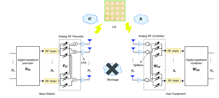
Figure 1: LIS-assisted mmWave hybrid downlink system.

II System Model and Problem Formulation

II-A System Model

We consider a point-to-point mmWave MIMO system as illustrated in Fig. 1, where the BS and the UE are equipped with a large number of antennas, and the LIS is deployed to assist the downlink data transmission from the BS to the UE. For simplicity, we assume that the direct link between the BS and the UE is blocked due to unfavorable propagation conditions. Nevertheless, our proposed scheme can be extended to the scenario in which a direct link between the BS and the UE is available. The BS is equipped with $N_{t}$ antennas and $R_{t}$ radio frequency (RF) chains, and the UE is equipped with $N_{r}$ antennas and $R_{r}$ RF chains, where $R_{t}\ll N_{t}$ and $R_{r}\ll N_{r}$. To exploit the channel diversity, multiple, say $N_{s}$, data streams are simultaneously sent from the BS to the UE, where $N_{s}\leq\min\{R_{t},R_{r}\}$. At the BS, a digital baseband precoder $\boldsymbol{F}_{\text{BB}}\in\mathbb{C}^{R_{t}\times N_{s}}$ is first applied to the transmitted signal $\boldsymbol{s}\in\mathbb{C}^{N_{s}}$, then followed by an analog RF beamformer $\boldsymbol{F}_{\text{RF}}\in\mathbb{C}^{N_{t}\times R_{t}}$. The transmitted signal can be written as

$$\boldsymbol{x}=\boldsymbol{F}_{\text{RF}}\boldsymbol{F}_{\text{BB}}\boldsymbol{s},$$ (1)

where $\boldsymbol{s}$ is assumed to satisfy $\mathbb{E}[\boldsymbol{s}\boldsymbol{s}^{H}]=\boldsymbol{I}$. Also, a transmit power constraint is placed on the hybrid precoding matrix $\boldsymbol{F}_{\text{RF}}\boldsymbol{F}_{\text{BB}}$, i.e. $\|\boldsymbol{F}_{\text{RF}}\boldsymbol{F}_{\text{BB}}\|_{F}^{2}\leq\rho$, $\rho$ is the transmit power.

The transmitted signal arrives at the UE via propagating through the BS-LIS-UE channel, where the LIS comprises $M$ passive reflecting elements and each element behaves like a single physical point which combines all the received signals and then re-scatters the combined signal with an adjustable phase shift [21]. Let $\boldsymbol{G}\in\mathbb{C}^{M\times N_{t}}$ denote the channel from the BS to the LIS, and $\boldsymbol{R}\in\mathbb{C}^{N_{r}\times M}$ denote the LIS-UE channel. Also, let $\phi_{m}\in[0,2\pi]$ denote the phase shift introduced by the $m$th element of the LIS, and

$$\boldsymbol{\Phi}\triangleq{\rm diag}(e^{j\phi_{1}},\cdots,e^{j\phi_{M}})\in\mathbb{C}^{M\times M}.$$ (2)

The signal received by the UE can thus be given as

$$\boldsymbol{y}=\boldsymbol{W}_{\text{BB}}^{H}\boldsymbol{W}_{\text{RF}}^{H}\boldsymbol{H}_{\rm eff}\boldsymbol{F}_{\text{RF}}\boldsymbol{F}_{\text{BB}}\boldsymbol{s}+\boldsymbol{W}_{\text{BB}}^{H}\boldsymbol{W}_{\text{RF}}^{H}\boldsymbol{n},$$ (3)

where $\boldsymbol{W}_{\text{RF}}\in\mathbb{C}^{N_{r}\times R_{r}}$ and $\boldsymbol{W}_{\text{BB}}\in\mathbb{C}^{R_{r}\times N_{s}}$ represent the analog combiner and the digital baseband combiner, respectively, $\boldsymbol{H}_{\rm eff}\triangleq\boldsymbol{R}\boldsymbol{\Phi}\boldsymbol{G}$ stands for the effective (i.e. cascade) channel from the BS to the UE, and $\boldsymbol{n}\in\mathbb{C}^{N_{r}}\sim\mathcal{CN}(0,\sigma^{2}\boldsymbol{I})$ denotes the additive white Gaussian noise.

In this paper, we assume that perfect channel state information (CSI) is known for joint transceiver and LIS design. Channel estimation for LIS-assisted systems is an important and challenging issue that has been studied in a variety of works, e.g. [29, 30, 31, 32]. In particular, [30, 31, 32] discussed how to estimate the channel for LIS-assisted mmWave systems. Suppose that the transmitted signal follows a Gaussian distribution. The achievable spectral efficiency can be expressed as [33]

$$R=\log_{2}{\rm det}\bigg{(}\boldsymbol{I}+ \frac{1}{\sigma^{2}}(\boldsymbol{W}_{\text{RF}}\boldsymbol{W}_{\text{BB}})^{\dagger}\boldsymbol{H}_{\rm{eff}}\boldsymbol{F}_{\text{RF}}\boldsymbol{F}_{\text{BB}}$$

$$\times\boldsymbol{F}_{\text{BB}}^{H}\boldsymbol{F}_{\text{RF}}^{H}\boldsymbol{H}_{\rm eff}^{H}(\boldsymbol{W}_{\text{RF}}\boldsymbol{W}_{\text{BB}})\bigg{)}.$$ (4)

where $\boldsymbol{A}^{\dagger}$ denotes the Moore-Penrose pseudo inverse of the matrix $\boldsymbol{A}$. It should be noted that since the analog precoder and combiner are implemented by analog phase shifters, entries of $\boldsymbol{F}_{\text{RF}}$ and $\boldsymbol{W}_{\text{RF}}$ have constant modulus.

II-B Channel Model

Due to the small wavelength, mmWave has limited ability to diffract around obstacles. As a result, mmWave channels exhibit a sparse multipath structure and are usually characterized by the Saleh-Valenzuela (SV) channel model [34, 35, 36, 37, 26]. Suppose uniform linear arrays (ULAs) are employed at the BS and the UE, and the LIS is a uniform planar array (UPA) consisting of a large number of reconfigurable passive elements. The BS-LIS channel $\boldsymbol{G}$ and the LIS-UE channel $\boldsymbol{R}$ can be given as

$$\boldsymbol{G}= \sqrt{\frac{N_{t}M}{P}}\sum_{i=1}^{P}\tilde{\alpha}_{i}\boldsymbol{a}_{R_{\rm LIS}}(\theta_{i}^{r},\eta_{i}^{r})\boldsymbol{a}_{T_{\rm BS}}^{H}(\gamma_{i}^{t}),$$ (5)

$$\boldsymbol{R}= \sqrt{\frac{MN_{r}}{L}}\sum_{i=1}^{L}\tilde{\beta}_{i}\boldsymbol{a}_{R_{\rm UE}}(\gamma_{i}^{r})\boldsymbol{a}_{T_{\rm LIS}}^{H}(\theta_{i}^{t},\eta_{i}^{t}),$$ (6)

where $P$ ($L$) is the total number of signal paths between the BS and the LIS (the LIS and the UE), $\theta_{i}^{r}$ ($\theta_{i}^{t}$) and $\eta_{i}^{r}$ ($\eta_{i}^{t}$) denote the azimuth and elevation angles of arrival (departure) associated with the LIS, $\gamma_{i}^{r}$ ($\gamma_{i}^{t}$) represents the angle of arrival (departure) associated with the UE (BS), $\tilde{\alpha}_{i}$ $(\tilde{\beta}_{i})$ is the complex channel gain, $\boldsymbol{a}_{R_{j}},j\in\{{\rm LIS,UE}\}$ and $\boldsymbol{a}_{T_{i}},i\in\{{\rm BS,LIS}\}$ denote the normalized array response vectors associated with the receiver and the transmitter, respectively. Specifically, for ULA with $N$ antennas, the normalized array response vector is given by

$$\boldsymbol{a}(\gamma)=\frac{1}{\sqrt{N}}[1\phantom{0}\cdots\phantom{0}e^{j\frac{2\pi d}{\lambda}(n-1)\sin(\gamma)}\phantom{0}\cdots\phantom{0}e^{j\frac{2\pi d}{\lambda}(N-1)\sin(\gamma)}]^{T},$$ (7)

where $d$ and $\lambda$ are the antenna spacing and the signal wavelength. For UPA with $M=M_{y}\times M_{z}$ elements, the normalized array response vector can be written as

$$\boldsymbol{a}(\theta,\eta)=\frac{1}{\sqrt{M}}[1\phantom{0}\cdots\phantom{0}e^{j\frac{2\pi d}{\lambda}((m_{1}-1)\cos(\eta)\sin(\theta)+(m_{2}-1)\sin(\eta))}$$

$$\cdots\phantom{0}e^{j\frac{2\pi d}{\lambda}((M_{y}-1)\cos(\eta)\sin(\theta)+(M_{z}-1)\sin(\eta))}]^{T}.$$ (8)

II-C Problem Formulation

Our objective is to jointly devise the hybrid precoding/combining matrices and the passive beamforming matrix $\boldsymbol{\Phi}$ to maximize the spectral efficiency (4):

$$\max_{\{\boldsymbol{F}_{\text{RF}},\boldsymbol{F}_{\text{BB}},\boldsymbol{W}_{\text{RF}},\boldsymbol{W}_{\text{BB}},\boldsymbol{\Phi}\}}\quad \log_{2}{\rm det}\big{(}\boldsymbol{I}+\frac{1}{\sigma^{2}}(\boldsymbol{W}_{\text{RF}}\boldsymbol{W}_{\text{BB}})^{\dagger}\boldsymbol{H}_{\rm{eff}}$$

$$\times\boldsymbol{F}_{\text{RF}}\boldsymbol{F}_{\text{BB}}\boldsymbol{F}_{\text{BB}}^{H}\boldsymbol{F}_{\text{RF}}^{H}\boldsymbol{H}_{\rm eff}^{H}(\boldsymbol{W}_{\text{RF}}\boldsymbol{W}_{\text{BB}})\big{)}$$

s.t. $$\|\boldsymbol{F}_{\text{RF}}\boldsymbol{F}_{\text{BB}}\|_{F}^{2}\leq\rho,$$

$$|\boldsymbol{F}_{\text{RF}}(i,j)|=|\boldsymbol{W}_{\text{RF}}(i,j)|=1,\quad\forall i,j,$$

$$\boldsymbol{H}_{\rm{eff}}=\boldsymbol{R}\boldsymbol{\Phi}\boldsymbol{G}$$

$$\boldsymbol{\Phi}={\rm diag}(e^{j\phi_{1}},\cdots,e^{j\phi_{M}}).$$ (9)

Such an optimization problem is challenging due to the non-convexity of the objective function and the per-element unit-modulus constraint placed on analog precoding and combining matrices.

To simplify the problem, we first ignore the constraint introduced by the hybrid analog/digital structure and consider a fully digital precoder/combiner. Let $\boldsymbol{F}\in\mathbb{C}^{N_{t}\times N_{s}}$ be a fully digital precoder which has the same size as the hybrid precoding matrix $\boldsymbol{F}_{\text{RF}}\boldsymbol{F}_{\text{BB}}$, and $\boldsymbol{W}\in\mathbb{C}^{N_{r}\times N_{s}}$ be a fully digital combiner which has the same size as the hybrid combining matrix $\boldsymbol{W}_{\text{RF}}\boldsymbol{W}_{\text{BB}}$. The problem (9) can be simplified as

$$\max_{\{\boldsymbol{F},\boldsymbol{W},\boldsymbol{\Phi}\}}\quad \log_{2}{\rm det}\big{(}\boldsymbol{I}+\frac{1}{\sigma^{2}}(\boldsymbol{W})^{\dagger}\boldsymbol{H}_{\rm{eff}}\boldsymbol{F}\boldsymbol{F}^{H}\boldsymbol{H}_{\rm eff}^{H}\boldsymbol{W}\big{)}$$

s.t. $$\|\boldsymbol{F}\|_{F}^{2}\leq\rho$$

$$\boldsymbol{H}_{\rm{eff}}=\boldsymbol{R}\boldsymbol{\Phi}\boldsymbol{G}$$

$$\boldsymbol{\Phi}={\rm diag}(e^{j\phi_{1}},\cdots,e^{j\phi_{M}}).$$ (10)

Once an optimal fully digital precoder/combiner is obtained, we can employ the manifold optimization-based method [38] to search for a hybrid precoding/combining matrix to approximate the optimal fully digital precoder/combiner. Such a strategy can be well justified because it has been shown in many previous studies [35, 38, 33, 36] that, due to the sparse scattering nature of mmWave channels, hybrid beamforming/combining with a small number of RF chains can asymptotically approach the performance of fully digital beamforming/combining for a sufficiently large number of antennas at the transceiver.

Given a fixed $\boldsymbol{\Phi}$ (i.e. $\boldsymbol{H}_{\rm{eff}}$), the optimal $\boldsymbol{F}$ and $\boldsymbol{W}$ can be obtained via the singular value decomposition (SVD) of $\boldsymbol{H}_{\rm eff}$. Define the effective channel’s ordered SVD as

$$\boldsymbol{H}_{\rm eff}=\boldsymbol{U}\boldsymbol{\Sigma}\boldsymbol{V}^{H}=\begin{matrix}[\boldsymbol{U}_{1}&\boldsymbol{U}_{2}]\end{matrix}\left[\begin{matrix}\boldsymbol{\Sigma}_{1}&\boldsymbol{0}\\ \boldsymbol{0}&\boldsymbol{\Sigma}_{2}\end{matrix}\right]\left[\begin{matrix}\boldsymbol{V}_{1}^{H}\\ \boldsymbol{V}_{2}^{H}\end{matrix}\right],$$ (11)

where $\boldsymbol{U}$ is an $N_{r}\times Q$ unitary matrix, $\boldsymbol{\Sigma}$ is a $Q\times Q$ diagonal matrix of singular values, $\boldsymbol{V}$ is an $N_{t}\times Q$ unitary matrix, in which $Q\triangleq{\rm rank}(\boldsymbol{H}_{\rm eff})$. The matrix $\boldsymbol{\Sigma}_{1}$ is of dimension $N_{s}\times N_{s}$ and $\boldsymbol{V}_{1}$ is of dimension $N_{t}\times N_{s}$. Then with a fixed $\boldsymbol{\Phi}$, the optimal solution to (10) is given as

$$\boldsymbol{F}_{\text{opt}}=\boldsymbol{V}_{1}\boldsymbol{\Lambda}^{1/2},\quad\boldsymbol{W}_{\text{opt}}=\boldsymbol{U}_{1},$$ (12)

where $\boldsymbol{\Lambda}={\rm diag}(p_{1},\ldots,p_{N_{s}})$, $p_{i}={\rm max}(1/\lambda-\sigma^{2}/\boldsymbol{\Sigma}_{1}^{2}(i,i),0),i=1,\ldots,N_{s}$ denotes the optimal amount of power allocated to the $i$th data stream, $1/\lambda$ is the water level satisfying $\sum_{i=1}^{N_{s}}p_{i}=\rho$. Thanks to the massive array gain provided by the LIS and large number of antennas at the BS, the effective signal-to-noise ratio (SNR) is large, in which case an equal power allocation scheme is near-optimal [35]. Therefore we can approximate $\boldsymbol{F}_{\text{opt}}$ as:

$$\boldsymbol{F}_{\text{opt}}\approx\sqrt{\frac{{\rho}}{N_{s}}}\boldsymbol{V}_{1}.$$ (13)

Substituting the optimal fully digital precoder and combiner into (10), we arrive at a problem which concerns only the optimization of the passive beamforming matrix $\boldsymbol{\Phi}$:

$$\max_{\boldsymbol{\Phi}}\quad \log_{2}{\rm det}\left(\boldsymbol{I}+\frac{\rho}{N_{s}\sigma^{2}}\boldsymbol{\Sigma}_{1}^{2}\right)$$

$${\rm s.t.}\quad \boldsymbol{\Phi}={\rm diag}(e^{j\phi_{1}},\cdots,e^{j\phi_{M}}).$$ (14)

The above objective function can be bounded by

$$\log_{2}{\rm det}\left(\boldsymbol{I}+\frac{\rho}{N_{s}\sigma^{2}}\boldsymbol{\Sigma}_{1}^{2}\right)\stackrel{{\scriptstyle(a)}}{{\leq}} N_{s}\log_{2}(1+\frac{\rho}{N_{s}^{2}\sigma^{2}}{\rm tr}(\boldsymbol{\Sigma}_{1}^{2}))$$

$$\stackrel{{\scriptstyle(b)}}{{\leq}} N_{s}\log_{2}(1+\frac{\rho}{N_{s}^{2}\sigma^{2}}{\rm tr}(\boldsymbol{H}_{\rm eff}\boldsymbol{H}_{\rm eff}^{H})),$$ (15)

where $(a)$ is due to Jensen’s inequality and $(b)$ becomes equality when $N_{s}=Q$. Therefore, alternatively, [24] proposed to maximize the bound of the spectral efficiency:

$$\max_{\boldsymbol{\Phi}}\quad {\rm tr}(\boldsymbol{H}_{\rm eff}\boldsymbol{H}_{\rm eff}^{H})$$

$${\rm s.t.}\quad \boldsymbol{\Phi}={\rm diag}(e^{j\phi_{1}},\cdots,e^{j\phi_{M}}).$$ (16)

Nevertheless, the objective of (16) does not consider the fairness among different singular values and thus results in a large condition number of $\boldsymbol{H}_{\rm eff}$. A large condition number indicates an unfavorable propagation condition since we prefer the power of the channel to be uniformly distributed over singular values to support multi-stream transmission [39]. To address this issue, we will develop a new approach to solve (14). Our proposed method obtains more balanced singular values of $\boldsymbol{\Sigma}_{1}$ which can help substantially improve the spectral efficiency, as suggested by our empirical results.

III Proposed Passive Beamforming Design Method

Optimizing (14) is much more challenging than directly optimizing the Frobenius-norm of ${\boldsymbol{H}}_{\rm eff}$, as the singular value can not be expressed by $\boldsymbol{H}_{\rm eff}$ in an explicit way. To address this difficulty, we exploit the structure of mmWave channels to gain insight into the SVD of the effective channel. Recall (5)–(6) and assume $|\beta_{1}|\geq|\beta_{2}|\geq\ldots\geq|\beta_{L}|$ and $|\alpha_{1}|\geq|\alpha_{2}|\geq\cdots\geq|\alpha_{P}|$, where $\alpha_{i}\triangleq\sqrt{\frac{N_{t}M}{P}}\tilde{\alpha}_{i}$, and $\beta_{i}\triangleq\sqrt{\frac{MN_{r}}{L}}\tilde{\beta}_{i}$. We will justify the order of $\{\beta_{l}\}$ and $\{\alpha_{p}\}$ later. The effective channel $\boldsymbol{H}_{\rm eff}=\boldsymbol{R}\boldsymbol{\Phi}\boldsymbol{G}$ can be written as

$$\boldsymbol{R}\boldsymbol{\Phi}\boldsymbol{G}$$

$$= \bigg{(}\sum_{i=1}^{L}\beta_{i}\boldsymbol{a}_{R_{\rm UE}}(\gamma_{i}^{r})\boldsymbol{a}_{T_{\rm LIS}}^{H}(\theta_{i}^{t},\eta_{i}^{t})\bigg{)}\boldsymbol{\Phi}$$

$$\quad\times\bigg{(}\sum_{j=1}^{P}\alpha_{j}\boldsymbol{a}_{R_{\rm LIS}}(\theta_{j}^{r},\eta_{j}^{r})\boldsymbol{a}_{T_{\rm BS}}^{H}(\gamma_{j}^{t})\bigg{)}$$

$$= \sum_{i=1}^{L}\sum_{j=1}^{P}\beta_{i}\alpha_{j}\boldsymbol{a}_{R_{\rm UE}}(\gamma_{i}^{r})\underbrace{\boldsymbol{a}_{T_{\rm LIS}}^{H}(\theta_{i}^{t},\eta_{i}^{t})\boldsymbol{\Phi}\boldsymbol{a}_{R_{\rm LIS}}(\theta_{j}^{r},\eta_{j}^{r})}_{d_{ij}}\boldsymbol{a}_{T_{\rm BS}}^{H}(\gamma_{j}^{t})$$

$$= \sum_{i=1}^{L}\sum_{j=1}^{P}\beta_{i}\alpha_{j}d_{ij}\boldsymbol{a}_{R_{\rm UE}}(\gamma_{i}^{r})\boldsymbol{a}_{T_{\rm BS}}^{H}(\gamma_{j}^{t})$$

$$= \boldsymbol{A}_{R_{\rm UE}}\boldsymbol{D}\boldsymbol{A}_{T_{\rm BS}}^{H},$$ (17)

where ${\boldsymbol{D}}$ is an $L\times P$ matrix with its $(i,j)$th entry given by ${\boldsymbol{D}(i,j)}=\beta_{i}\alpha_{j}d_{ij}$, and $d_{ij}$ is defined as

$$d_{ij}\triangleq \boldsymbol{a}_{T_{\rm LIS}}^{H}(\theta_{i}^{t},\eta_{i}^{t})\boldsymbol{\Phi}\boldsymbol{a}_{R_{\rm LIS}}(\theta_{j}^{r},\eta_{j}^{r})$$

$$= \boldsymbol{v}^{H}(\boldsymbol{a}_{T_{\rm LIS}}^{\ast}(\theta_{i}^{t},\eta_{i}^{t})\circ\boldsymbol{a}_{R_{\rm LIS}}(\theta_{j}^{r},\eta_{j}^{r}))$$

$$= \boldsymbol{v}^{H}\boldsymbol{p}^{ij}$$ (18)

with $\circ$ stands for the Hadamard (elementwise) product, ${\boldsymbol{v}\triangleq{\text{diag}}({\boldsymbol{\Phi}^{H}})}$, and ${\boldsymbol{p}}^{ij}\triangleq(\boldsymbol{a}_{T_{\rm LIS}}^{\ast}(\theta_{i}^{t},\eta_{i}^{t})\circ\boldsymbol{a}_{R_{\rm LIS}}(\theta_{j}^{r},\eta_{j}^{r}))$. Here $d_{ij}$ is referred to as the passive beamforming gain associated with the $(j,i)$th BS-LIS-UE composite path which is composed of the $j$th path from the BS to the LIS and the $i$th path from the LIS to the UE.

Also, $\boldsymbol{A}_{R_{\rm UE}}$ and $\boldsymbol{A}_{T_{\rm BS}}$ in (17) are respectively defined as

$$\boldsymbol{A}_{R_{\rm UE}}\triangleq [\boldsymbol{a}_{R_{\rm UE}}(\gamma_{1}^{r})\phantom{0}\cdots\phantom{0}\boldsymbol{a}_{R_{\rm UE}}(\gamma_{L}^{r})],$$

$$\boldsymbol{A}_{T_{\rm BS}}\triangleq [\boldsymbol{a}_{T_{\rm BS}}(\gamma_{1}^{t})\phantom{0}\cdots\phantom{0}\boldsymbol{a}_{T_{\rm BS}}(\gamma_{P}^{t})].$$ (19)

For ULA with $N$ antennas, it can be easily verified that

$$|{\boldsymbol{a}}^{H}(\gamma_{i}){\boldsymbol{a}}(\gamma_{j})|\rightarrow 0,\quad N\rightarrow\infty$$ (20)

for any $\sin(\gamma_{i})-\sin(\gamma_{j})\neq 0$. This asymptotic orthogonality also holds valid for other array geometries such as UPA [40]. Therefore when $N_{t}$ and $N_{r}$ are sufficiently large, $\boldsymbol{A}_{R_{\rm UE}}$ and $\boldsymbol{A}_{T_{\rm BS}}$ can be considered as orthonormal matrices in which the columns vectors form an orthonormal set (each column vector has unit norm and is orthogonal to all the other column vectors). If the phase shift vector $\boldsymbol{v}$ is properly devised such that the off-diagonal elements of $\boldsymbol{D}$ are small relative to entries on the main diagonal, then $\boldsymbol{H}_{\rm eff}=\boldsymbol{A}_{R_{\rm UE}}\boldsymbol{D}\boldsymbol{A}_{T_{\rm BS}}^{H}$ can be treated as an approximation of the truncated SVD of $\boldsymbol{H}_{\rm eff}$, in which case the optimization problem (14) turns into

$$\max_{\boldsymbol{v}}\quad \sum_{i=1}^{{N_{s}}}\log_{2}\left(1+\frac{\rho}{N_{s}\sigma^{2}}|\boldsymbol{D}(i,i)|^{2}\right)$$

$${\rm s.t.}\quad \boldsymbol{D}(i,i)=\alpha_{i}\beta_{i}d_{ii},\quad\forall i\in\{1,\cdots,N_{s}\},$$

$$d_{ii}=\boldsymbol{v}^{H}\boldsymbol{p}^{ii},$$

$$|d_{ij}|=|\boldsymbol{v}^{H}\boldsymbol{p}^{ij}|<\tau,\quad\forall i\neq j,$$

$$\boldsymbol{v}=[e^{j\phi_{1}}\phantom{0}\cdots\phantom{0}e^{j\phi_{M}}]^{H},$$ (21)

where $\tau$ is a small positive value and the constraint $|d_{ij}|<\tau$ is to make sure that $\boldsymbol{D}$ is approximately a non-square diagonal matrix such that $\boldsymbol{H}_{\rm eff}=\boldsymbol{A}_{R_{\rm UE}}\boldsymbol{D}\boldsymbol{A}_{T_{\rm BS}}^{H}$ approximates a truncated SVD of $\boldsymbol{H}_{\rm eff}$. One could question that such a constraint (i.e. $|d_{ij}|<\tau,\forall i\neq j$) not only complicates the problem, but also confines the solution space of $\boldsymbol{v}$, and thus may prevent from achieving a higher spectral efficiency. We will show that this constraint can be ignored and this omission does not affect the validity of our proposed solution. Specifically, we focus on solving

$$\max_{\boldsymbol{v}}\quad \sum_{i=1}^{{N_{s}}}\log_{2}\left(1+\frac{\rho}{N_{s}\sigma^{2}}|\boldsymbol{D}(i,i)|^{2}\right)$$

$${\rm s.t.}\quad \boldsymbol{D}(i,i)=\alpha_{i}\beta_{i}d_{ii},\quad\forall i\in\{1,\cdots,N_{s}\},$$

$$d_{ii}=\boldsymbol{v}^{H}\boldsymbol{p}^{ii},$$

$$\boldsymbol{v}=[e^{j\phi_{1}}\phantom{0}\cdots\phantom{0}e^{j\phi_{M}}]^{H},$$ (22)

and we will show that for a sufficiently large $M$, the solution to (22) automatically ensures that off-diagonal entries of $\boldsymbol{D}$ are small relative to entries on its main diagonal. Thus it is expected that solving (22) leads to an effective solution of (14).

III-A Manifold-Based Method for Passive Beamforming Design

In this subsection, we develop a manifold-based method to solve (22). Note that other methods such as the semidefinite relaxation (SDR) method, the block coordinate descent (BCD) method [41] and the penalty dual decomposition (PDD) method [42] can also be employed to address (22). The reason we choose to use the manifold optimization technique is that it achieves a good balance between the computational complexity and the performance. Recalling that $\boldsymbol{D}(i,i)=\alpha_{i}\beta_{i}\boldsymbol{v}^{H}\boldsymbol{p}^{ii}$, the optimization (22) can be rewritten as

$$\max_{\boldsymbol{v}}\quad \sum_{i=1}^{{N_{s}}}\log_{2}(1+a_{i}\boldsymbol{v}^{H}\boldsymbol{P}^{ii}\boldsymbol{v})$$

s.t. $$\boldsymbol{v}=[e^{j\phi_{1}}\phantom{0}\cdots\phantom{0}e^{j\phi_{M}}]^{H},$$ (23)

where $\boldsymbol{P}^{ii}\triangleq\boldsymbol{p}^{ii}(\boldsymbol{p}^{ii})^{H}$, and $a_{i}\triangleq\frac{\rho}{N_{s}\sigma^{2}}|\alpha_{i}\beta_{i}|^{2}$. The main difficulty involved in solving (23) is the non-convex unit modulus constraint. We employ the manifold optimization technique to address this difficulty. The search space of (23) can be regarded as the product of $M$ complex circles, i.e.,

$$\underbrace{\mathcal{S}\times\mathcal{S}\cdots\times\mathcal{S}}_{M\;{\rm times}},$$ (24)

where $\mathcal{S}\triangleq\{u\in\mathbb{C}:u^{H}u=1\}$ is one complex circle[43]. The product of such $M$ circles is a submanifold of $\mathbb{C}^{M}$, known as the complex circle manifold (CCM) [44], which is defined as

$$\mathcal{M}=\mathcal{S}^{M}\triangleq\{\boldsymbol{u}\in\mathbb{C}^{M}:|u_{i}|=1,i=1,2,\cdots,M\}.$$ (25)

More background on optimization on manifolds can be found in [44].

For a smooth real-valued objective function on some manifold, many classical line-search algorithms such as the gradient descent method can be applied with certain modifications [45]. We start with some basic definitions. The tangent space ${\mathcal{T}_{\boldsymbol{v}^{k}}\mathcal{M}}$ is the set consisting of all tangent vectors to $\mathcal{M}$ at the point $\boldsymbol{v}^{k}$ [44]. Here, the tangent space of the complex circle manifold admits a closed-form expression, i.e.,

$${\mathcal{T}_{\boldsymbol{v}^{k}}\mathcal{M}}=\{\boldsymbol{z}\in\mathbb{C}^{M}:\Re\{\boldsymbol{z}\circ(\boldsymbol{v}^{k})^{\ast}\}=\boldsymbol{0}\},$$ (26)

where $\circ$ denotes the Hadamard product. Since the descent is performed on the manifold, we need to find the direction of the greatest decrease from the tangent space, which is known as the negative Riemannian gradient. For the complex circle manifold, the Riemannian gradient of the objective function $f(\boldsymbol{v})\triangleq-\sum_{i=1}^{{N_{s}}}\log(1+a_{i}\boldsymbol{v}^{H}\boldsymbol{P}^{ii}\boldsymbol{v})$ at the point $\boldsymbol{v}^{k}$ is a tangent vector $\nabla_{{\mathcal{M}}}f(\boldsymbol{v}^{k})$ given by [44]

$$\nabla_{{\mathcal{M}}}f(\boldsymbol{v}^{k})= {\rm Proj}_{\mathcal{T}_{\boldsymbol{v}^{k}}\mathcal{M}}(\nabla f(\boldsymbol{v}^{k}))$$

$$= \nabla f(\boldsymbol{v}^{k})-\Re\{\nabla f(\boldsymbol{v}^{k})\circ(\boldsymbol{v}^{k})^{\ast}\}\circ\boldsymbol{v}^{k},$$ (27)

where ${\rm Proj}(\cdot)$ is the orthogonal projection operator and the Euclidean gradient $\nabla f(\boldsymbol{v}^{k})$ is given as

$$\nabla f(\boldsymbol{v}^{k})=-\sum_{i=1}^{N_{s}}\frac{1}{\ln 2}\frac{2a_{i}\boldsymbol{P}^{ii}\boldsymbol{v}^{k}}{1+a_{i}(\boldsymbol{v}^{k})^{H}\boldsymbol{P}^{ii}\boldsymbol{v}^{k}}.$$ (28)

After we obtain the Riemannian gradient, we can transplant many line-search algorithms, such as the gradient descent method, from the Euclidean spaces to the Riemannian manifolds [45]. Specifically, we update $\boldsymbol{v}^{k}$ with a step $\varpi^{k}$

$$\boldsymbol{\bar{v}}^{k}=\boldsymbol{v}^{k}-\varpi^{k}\nabla_{{\mathcal{M}}}f(\boldsymbol{v}^{k}),$$ (29)

where $\varpi^{k}$ is chosen as the Armijo step size [44]. In general, $\boldsymbol{\bar{v}}^{k}$ does not lie in the complex circle manifold, thus the retraction is needed to map the updated point $\boldsymbol{\bar{v}}^{k}$ on the tangent space $\mathcal{T}_{\boldsymbol{v}^{k}}\mathcal{M}$ onto the complex circle manifold $\mathcal{M}$ with a local rigidity condition preserving the gradients at $\boldsymbol{v}^{k}$. In this case, the retraction operator is defined as [44]

$$\boldsymbol{v}^{k+1}={\rm R}(\boldsymbol{\bar{v}}^{k})\triangleq\boldsymbol{\bar{v}}^{k}\circ\frac{1}{|\boldsymbol{\bar{v}}^{k}|}.$$ (30)

The algorithm above is summarized in Algorithm 1, which is guaranteed to converge to a critical point of (23) [44].

Algorithm 1 Proposed Algorithm for Solving (23)

1:  Initialize $\boldsymbol{v}^{0}\in\mathcal{M}$ and give a pre-defined threshold $\varepsilon$.

2:  repeat

3:     Compute the Euclidean gradient $\nabla f(\boldsymbol{v}^{k})$ using (28);

4:     Compute the Riemannian gradient $\nabla_{{\mathcal{M}}}f(\boldsymbol{v}^{k})$ with (27);

5:     Choose an Armijo step size $\varpi^{k}$ ([44], see section 4.2.2);

6:     Update $\boldsymbol{\bar{v}}^{k}=\boldsymbol{v}^{k}-\varpi^{k}\nabla_{{\mathcal{M}}}f(\boldsymbol{v}^{k})$;

7:     Update $\boldsymbol{v}^{k+1}={\rm R}(\boldsymbol{\bar{v}}^{k})$ using (30);

8:  until the gap of the objective function values between two iterations is smaller than $\varepsilon$ .

9:  Obtain the optimal solution ${\boldsymbol{v}}^{\star}$.

III-B Discussions

Next, we discuss for a sufficiently large $M$, why the constraint $|d_{i,j}|<\tau,\forall i\neq j$ in (21) can be ignored and the solution to (22) yields small values of $\{d_{ij},\forall i\neq j\}$.

Define $k\triangleq\frac{2\pi d}{\lambda}$, $f(\theta,\eta)\triangleq\cos(\eta)\sin(\theta)$, $g(\eta)\triangleq\sin(\eta)$, and $\boldsymbol{\bar{p}}^{ij}\triangleq\sqrt{M}\boldsymbol{p}^{ij}$. We have

$$\boldsymbol{\bar{p}}^{ij}\triangleq \sqrt{M}(\boldsymbol{a}_{T_{\rm LIS}}^{\ast}(\theta_{i}^{t},\eta_{i}^{t})\odot\boldsymbol{a}_{R_{\rm LIS}}(\theta_{j}^{r},\eta_{j}^{r}))$$

$$= \frac{1}{\sqrt{M}}[1\phantom{0}\ldots\phantom{0}e^{jk((m_{1}-1)(\Delta f_{ij})+(m_{2}-1)(\Delta g_{ij})}\phantom{0}$$

$$\quad\quad\quad\ldots\phantom{0}e^{jk((M_{y}-1)(\Delta f_{ij})+(M_{z}-1)(\Delta g_{ij})}]^{T},$$ (31)

where $\Delta f_{ij}\triangleq f(\theta_{j}^{r},\eta_{j}^{r})-f(\theta_{i}^{t},\eta_{i}^{t})$ and $\Delta g_{ij}\triangleq g(\eta_{j}^{r})-g(\eta_{i}^{t})$. Therefore, we can calculate $|(\boldsymbol{\bar{p}}^{ij})^{H}\boldsymbol{\bar{p}}^{mn}|$ as

$$|(\boldsymbol{\bar{p}}^{ij})^{H}\boldsymbol{\bar{p}}^{mn}|$$

$$= \frac{1}{M}\left|\sum_{m_{1}=1}^{M_{y}}\sum_{m_{2}=1}^{M_{z}}e^{jk((m_{1}-1)(\Delta F_{ijmn})+(m_{2}-1)(\Delta G_{ijmn})}\right|$$

$$= \frac{1}{M}\left|\frac{\sin\left(\frac{1}{2}kM_{y}\Delta F_{ijmn}\right)}{\sin\left(\frac{1}{2}k\Delta F_{ijmn}\right)}\frac{\sin\left(\frac{1}{2}kM_{z}\Delta G_{ijmn}\right)}{\sin\left(\frac{1}{2}k\Delta G_{ijmn}\right)}\right|,$$ (32)

where $\Delta F_{ijmn}\triangleq\Delta f_{mn}-\Delta f_{ij}$ and $\Delta G_{ijmn}\triangleq\Delta g_{mn}-\Delta g_{ij}$. Due to the random distribution of AoA and AoD parameters, we have $\Delta F_{ijmn}\neq 0$ or $\Delta G_{ijmn}\neq 0$ for any $\{m,n\}\neq\{i,j\}$ with probability one. Thus we have

$$\lim_{M\rightarrow\infty}\mid(\boldsymbol{\bar{p}}^{ij})^{H}\boldsymbol{\bar{p}}^{mn}\mid=0,\forall m\neq i\parallel n\neq j,$$ (33)

where $\parallel$ denotes the OR logic operation which means either $m\neq i$ or $n\neq j$ is true. Also, it is easy to verify that $(\boldsymbol{\bar{p}}^{ij})^{H}\boldsymbol{\bar{p}}^{ij}=1$.

Define $\mathcal{A}\triangleq\{\boldsymbol{\bar{p}}^{ii}:i=1,\ldots,N_{s}\}$ and $\mathcal{B}\triangleq\{\boldsymbol{\bar{p}}^{mn}:\{m,n\}\in\mathcal{E}\}$, where $\mathcal{E}\triangleq\mathcal{U}-\mathcal{I}$, in which

$$\mathcal{U}\triangleq \{\{m,n\}:m\in\{1,\ldots,L\},n\in\{1,\ldots,P\}\}$$ (34)

$$\mathcal{I}\triangleq \{\{i,i\}:i\in\{1,\ldots,N_{s}\}\}$$ (35)

Let $\mathcal{C}\triangleq\{\boldsymbol{c}_{u}\}_{u=1}^{M-LP}$ denote an orthonormal set whose vectors are orthogonal to those vectors in $\mathcal{A}\cup\mathcal{B}$. Clearly, the set of vectors in $\mathcal{D}\triangleq\mathcal{A}\cup\mathcal{B}\cup\mathcal{C}$ form an orthonormal basis of $\mathbb{C}^{M}$. Hence, any vector in $\mathbb{C}^{M}$ can be expressed as a sum of the basis vectors scaled

$$\boldsymbol{v}=\sum_{i=1}^{N_{s}}k_{ii}\boldsymbol{\bar{p}}^{ii}+\sum_{\{m,n\}\in\mathcal{E}}k_{mn}\boldsymbol{\bar{p}}^{mn}+\sum_{u=1}^{M-LP}k_{u}\boldsymbol{c}_{u}.$$ (36)

It should be noted that

$$M=\boldsymbol{v}^{H}\boldsymbol{v}= \sum_{i=1}^{N_{s}}|k_{ii}|^{2}+\sum_{\{m,n\}\in\mathcal{E}}|k_{mn}|^{2}+\sum_{u=1}^{M-LP}|k_{u}|^{2}.$$ (37)

Substituting (36) into the objective function of (23), we have

$$\sum_{i=1}^{N_{s}}\log_{2}(1+a_{i}|\boldsymbol{v}^{H}\boldsymbol{p}^{ii}|^{2})$$

$$= \sum_{i=1}^{N_{s}}\log_{2}\bigg{(}1+a_{i}\bigg{|}\bigg{(}\sum_{i=1}^{N_{s}}k_{ii}\boldsymbol{\bar{p}}^{ii}+\sum_{\{m,n\}\in\mathcal{E}}k_{mn}\boldsymbol{\bar{p}}^{mn}$$

$$+\sum_{u=1}^{M-LP}k_{u}\boldsymbol{c}_{u}\bigg{)}^{H}\boldsymbol{p}^{ii}\bigg{|}^{2}\bigg{)}$$

$$= \sum_{i=1}^{N_{s}}\log_{2}\left(1+\frac{a_{i}}{M}|k_{ii}|^{2}\right).$$ (38)

Therefore (23) can be re-expressed as

$$\max_{\{k_{ii},k_{mn},k_{u}\}}\quad \sum_{i=1}^{N_{s}}\log_{2}(1+\frac{a_{i}}{M}|k_{ii}|^{2})$$

s.t. $$\sum_{i=1}^{N_{s}}|k_{ii}|^{2}\leq M,$$

$$\boldsymbol{v}=[e^{j\phi_{1}}\phantom{0}\cdots\phantom{0}e^{j\phi_{M}}]^{H},$$

$$\boldsymbol{v}=\sum_{i=1}^{N_{s}}k_{ii}\boldsymbol{\bar{p}}^{ii}+\sum_{\{m,n\}\in\mathcal{E}}k_{mn}\boldsymbol{\bar{p}}^{mn}+\sum_{u=1}^{M-LP}k_{u}\boldsymbol{c}_{u}.$$ (39)

If no unit modulus constraint is placed on the phase shift vector $\boldsymbol{v}$, then it is clear that the objective function value of (39) is maximized when $\sum_{i=1}^{N_{s}}|k_{ii}|^{2}=M$, which means that $k_{mn}=0,\forall\{m,n\}\in\mathcal{E}$ and $k_{u}=0$. As a result, we have

$$d_{mn}=(\boldsymbol{v}^{\star})^{H}\boldsymbol{p}^{mn}=\left(\sum_{i=1}^{N_{s}}k_{ii}\boldsymbol{\bar{p}}^{ii}\right)^{H}\boldsymbol{p}^{mn}=0\quad\forall\{m,n\}\in\mathcal{E}$$ (40)

Hence the solution to (39) or (23), $\boldsymbol{v}^{\star}$, yields exactly zero off-diagonal entries of $\boldsymbol{D}$. With the unit modulus constraint $\boldsymbol{v}=[e^{j\phi_{1}}\phantom{0}\cdots\phantom{0}e^{j\phi_{M}}]^{H}$, $\sum_{i=1}^{N_{s}}|k_{ii}|^{2}$ will not be exactly equal to $M$ but the solution will force $\sum_{i=1}^{N_{s}}|k_{ii}|^{2}$ to be close to $M$ as much as possible in order to obtain a maximum objective function value. As a result, the values of $\{|k_{mn}|\},\forall\{m,n\}\in\mathcal{E}$ are small relative to $\{|k_{ii}|,i=1,\ldots,N_{s}\}$. Note that we have

$$d_{pq}=(\boldsymbol{v}^{\star})^{H}\boldsymbol{p}^{pq}$$

$$= \left(\sum_{i=1}^{N_{s}}k_{ii}\boldsymbol{\bar{p}}^{ii}+\sum_{\{m,n\}\in\mathcal{E}}k_{mn}\boldsymbol{\bar{p}}^{mn}+\sum_{u=1}^{M-LP}k_{u}\boldsymbol{c}_{u}\right)^{H}\boldsymbol{p}^{pq}$$

$$= \begin{cases}\frac{k_{pq}}{\sqrt{M}}&q\neq p\\ \frac{k_{pp}}{\sqrt{M}}&q=p\end{cases}$$ (41)

Therefore the optimal solution to (23) yields an approximately diagonal matrix $\boldsymbol{D}$ whose off-diagonal entries $\{d_{ij},i\neq j\}$ are small relative to its diagonal entries $\{d_{ii},i=1,\ldots,N_{s}\}$.

III-C Ordering of $\{\beta_{i}\}$ and $\{\alpha_{i}\}$

Note that we assumed a decreasing order of the path gains $\{\beta_{i}\}$ and $\{\alpha_{i}\}$ earlier in this paper, i.e. $|\beta_{1}|\geq|\beta_{2}|\geq\ldots\geq|\beta_{L}|$ and $|\alpha_{1}|\geq|\alpha_{2}|\geq\cdots\geq|\alpha_{P}|$. Nevertheless, from (22), we can see that different orders of $\{\beta_{i}\}$ and $\{\alpha_{i}\}$ may lead to different solutions and thus different performance, and it is unclear whether arranging the path gains $\{\beta_{i}\}$ and $\{\alpha_{i}\}$ in a decreasing order is a good choice. To gain an insight into this problem, let us examine the optimization (39) which is a variant of (22). As discussed above, if we ignore the unit-modulus constraint placed on $\boldsymbol{v}$, (39) can be simplified as a conventional power allocation problem:

$$\max_{\{\tilde{k}_{ii}\}}\quad \sum_{i=1}^{N_{s}}\log_{2}(1+a_{i}|\tilde{k}_{ii}|^{2})$$

s.t. $$\sum_{i=1}^{N_{s}}|\tilde{k}_{ii}|^{2}\leq 1,$$ (42)

where $\tilde{k}_{ii}\triangleq\frac{k_{ii}}{\sqrt{M}}$. Recall that $a_{i}=\frac{\rho}{N_{s}\sigma^{2}}|\alpha_{i}\beta_{i}|^{2}$, where $\alpha_{i}=\sqrt{\frac{N_{t}M}{P}}\tilde{\alpha}_{i}$, and $\beta_{i}=\sqrt{\frac{N_{r}M}{L}}\tilde{\beta}_{i}$. Thanks to the large dimensions of $N_{t}$, $N_{r}$, and $M$, it can be expected that the effective signal-to-noise ratios (SNRs) $\{a_{i}\}$ have large values even the nominal SNR $\frac{\rho}{\sigma^{2}}$ is small. It is well-known that in the high SNR regime, it is approximately optimal to equally allocate power to different data streams. Therefore the question is how to arrange the orders of $\{\beta_{i}\}$ and $\{\alpha_{i}\}$ such that $\sum_{i=1}^{N_{s}}\log_{2}(1+a_{i}/N_{s})$ can be maximized.

Let $\{\tau_{l}\}_{l=1}^{L}$ be a permutation of the set $\{1,\ldots,L\}$ and $\{\pi_{p}\}_{p=1}^{P}$ a permutation of the set $\{1,\ldots,P\}$. We can write

$$S\triangleq \sum_{i=1}^{N_{s}}\log_{2}(1+a_{i}/N_{s})=\sum_{k=1}^{N_{s}}\log_{2}(1+e|\alpha_{\pi_{k}}|^{2}|\beta_{\tau_{k}}|^{2})$$

$$= \sum_{k=1}^{N_{s}}\log_{2}(|\alpha_{\pi_{k}}|^{2})+\sum_{k=1}^{N_{s}}\log_{2}\left(\frac{1}{|\alpha_{\pi_{k}}|^{2}}+e|\beta_{\tau_{k}}|^{2}\right)$$

$$\triangleq S_{1}+S_{2}.$$ (43)

where $e\triangleq\frac{\rho}{N_{s}^{2}\sigma^{2}}$. We see that $S_{1}$ is a constant once $\{\alpha_{\pi_{k}}\}_{k=1}^{N_{s}}$ is determined. Hence, we focus on the value of $S_{2}$. Note that

$$2^{S_{2}}=\prod_{k=1}^{N_{s}}\left(\frac{1}{|\alpha_{\pi_{k}}|^{2}}+e|\beta_{\tau_{k}}|^{2}\right).$$ (44)

Without loss of generality, we assume

$$\frac{1}{|\alpha_{\pi_{1}}|^{2}}\leq\frac{1}{|\alpha_{\pi_{2}}|^{2}}\leq\cdots\leq\frac{1}{|\alpha_{\pi_{N_{s}}}|^{2}}.$$ (45)

Clearly, according to the dual rearrangement inequality [46], $S_{2}$ attains its maximum if and only if

$$|\beta_{\tau_{1}}|^{2}\geq|\beta_{\tau_{2}}|^{2}\geq\cdots\geq|\beta_{\tau_{N_{s}}}|^{2}.$$ (46)

This means that similar to $\{\alpha_{\pi_{k}}\}_{k=1}^{N_{s}}$, $\{|\beta_{\tau_{k}}|\}_{k=1}^{N_{s}}$ should also be arranged in a decreasing order. This explains why we arrange the path gains of $\{\beta_{i}\}$ and $\{\alpha_{i}\}$ in a descending order.

IV Hybrid Precoding/Combining Design

After obtaining the passive beamforming matrix $\boldsymbol{\Phi}^{\star}$, we conduct the SVD of $\boldsymbol{H}^{\star}$, i.e. $\boldsymbol{H}^{\star}=\boldsymbol{R}\boldsymbol{\Phi}^{\star}\boldsymbol{G}=\boldsymbol{U}^{\star}\boldsymbol{\Sigma}^{\star}(\boldsymbol{V}^{\star})^{H}$ and the optimal precoder/combiner can be obtained via (12). As discussed earlier in this paper, we search for an analog precoding (combining) matrix $\boldsymbol{F}_{\text{RF}}$ ($\boldsymbol{W}_{\text{RF}}$) and a baseband precoding (combining) matrix $\boldsymbol{F}_{\text{BB}}$ ($\boldsymbol{W}_{\text{BB}}$) to approximate the optimal precoder (combiner) $\boldsymbol{F}_{\text{opt}}$ ($\boldsymbol{W}_{\text{opt}}$). In the following, we focus our discussion on the hybrid precoding design as the extension to the hybrid combining design is similar. Such a problem can be formulated as [38]

$$\min_{\boldsymbol{w}\in{\mathcal{M}_{2}},\boldsymbol{F}_{\rm BB}}\|\boldsymbol{F}_{\rm opt}-\boldsymbol{F}_{\rm RF}\boldsymbol{F}_{\rm BB}\|_{F}^{2},$$ (47)

where $\boldsymbol{w}\triangleq{\rm vec}(\boldsymbol{F}_{\rm RF})$ and the search space is a complex circle manifold defined as $\mathcal{M}_{2}\triangleq\mathcal{S}^{N_{t}R_{t}}$. Specifically, we adopt the fast manifold-based optimization method in [38] to solve (47), where we optimize $\boldsymbol{F}_{\text{RF}}$ and $\boldsymbol{F}_{\text{BB}}$ in an alternating manner. The detailed procedure can be found in [38] and thus omitted here. It should be noted that the method is guaranteed to converge to a critical point [38, 44] and has a computational complexity at the order of $\mathcal{O}(N_{t}R_{t}N_{s}L_{2})$, where $L_{2}$ is the number of iterations required to converge.

Algorithm 2 Proposed Algorithm for Joint Transceiver and LIS Design

0:   $\boldsymbol{R}$, $\boldsymbol{G}$, $N_{s}$, $R_{t}$, $R_{r}$, $\rho$, $\sigma^{2}$; First step

1:  Optimizing $\boldsymbol{\Phi}^{\star}$ by Algorithm 1 developed in Subsection III-A; Second step

2:  Compute the optimal precoding and combining matrices, i.e. $\boldsymbol{F}_{\rm opt}$ and $\boldsymbol{W}_{\rm opt}$, using (12)

3:  Obtain hybrid precoding and combining matrices, i.e. $\boldsymbol{F}_{\rm BB}$, $\boldsymbol{F}_{\rm RF}$ $\boldsymbol{W}_{\rm BB}$ and $\boldsymbol{W}_{\rm RF}$, via the manifold-based method discussed in Section IV;

3:  $\boldsymbol{\Phi}^{\star}$, $\boldsymbol{F}_{\rm BB}$, $\boldsymbol{F}_{\rm RF}$, $\boldsymbol{W}_{\rm BB}$, and $\boldsymbol{W}_{\rm RF}$.

V Summary and Discussions

First of all, we would like to clarify that different from other state-of-the-art methods [25, 24], our proposed method is designed specifically for mmWave systems. It relies on the sparse scattering structure of mmWave channels to obtain a good approximation of the SVD of the effective channel. On the other hand, as will be shown in the subsequent analysis and simulation results, utilizing the inherent sparse structure of mmWave channels enables us to achieve a better tradeoff between the spectral efficiency performance and the computational complexity.

V-A Computational Complexity Analysis

For clarity, the proposed algorithm is summarized in Algorithm 2. Specifically, our proposed algorithm consists of two steps. The first step aims to obtain LIS’s reflection coefficients via solving the passive beamforming optimization problem (23). A manifold-based method, i.e. Algorithm 1, is developed. The dominant operation for Algorithm 1 at each iteration is to calculate the Euclidean gradient (28), which has a computational complexity at the order of $\mathcal{O}(M)$. Note that $\boldsymbol{P}^{ii}=\boldsymbol{p}^{ii}(\boldsymbol{p}^{ii})^{H}$, and thus calculating $(\boldsymbol{p}^{ii})^{H}\boldsymbol{v}$ is enough to obtain (28). Therefore the first step involves a computational complexity of $\mathcal{O}(ML_{1})$, where $L_{1}$ denotes the number of iterations required to converge. The second step solves a hybrid beamforming problem which involves calculating the optimal precoder/combiner and searching for an analog precoding (combining) matrix and a baseband precoding (combining) matrix to approximate the optimal precoder (combiner). The optimal precoder/combiner can be obtained by performing the SVD of the effective channel, whose complexity is at the order of $\mathcal{O}(N_{r}N_{t}\min(N_{r},N_{t}))$. The proposed manifold-based algorithm for finding the analog/diginal precoding (combining) matrices, as discussed in the previous section, has a complexity of $\mathcal{O}(N_{r}R_{r}N_{s}L_{2}+N_{t}R_{t}N_{s}L_{2})$, where $L_{2}$ denotes the number of iterations required to converge. Thus, the overall computational complexity of our proposed algorithm is at the order of $\mathcal{O}(ML_{1}+N_{r}N_{t}\min(N_{r},N_{t})+N_{r}R_{r}N_{s}L_{2}+N_{t}R_{t}N_{s}L_{2})$.

Note that there is no alternating process between these two steps. We only need to execute each step once for our proposed algorithm. Since each step of our proposed algorithm is ensured to converge, the convergence of our proposed algorithm is guaranteed.

V-B Computational Complexity Comparison

In this subsection, we compare our proposed method with some state-of-the-art methods developed for spectral efficiency optimization for IRS-aided MIMO systems. Note that these methods are not specially designed to mmWave systems with hybrid precoding/combining structures. To apply them to our problem, a similar two-step procedure is required. Let us first consider the alternating optimization (AO)-based algorithm [25]. In the first step, the AO-based algorithm [25] is used to optimize the LIS’s reflection coefficients $\boldsymbol{\Phi}$ and the transmit covariance matrix $\boldsymbol{Q}$. The first step involves a computational complexity at the order of $\mathcal{O}(N_{r}N_{t}(M+\min(N_{r},N_{t}))L+((3N_{r}^{3}+2N_{r}^{2}N_{t}+N_{t}^{2})M+N_{r}N_{t}\min(N_{r},N_{t}))I)$, where $L$ is the number of realizations for initialization and $I$ denotes the number of outer iterations [25]. Note that the first step requires to calculate the SVD of the effective channel. Hence the optimal precoder/combiner can be directly obtained without involving additional computational complexity. In the second step, similar to our work, we resort to the manifold-based algorithm to find the hybrid precoder and combiner to approximate the optimal precoder/combiner, which involves a same computational complexity at the order of $\mathcal{O}(N_{r}R_{r}N_{s}L_{2}+N_{t}R_{t}N_{s}L_{2})$. Therefore the overall computational complexity of the AO-based algorithm [25] is at the order of $\mathcal{O}(N_{r}N_{t}(M+\min(N_{r},N_{t}))L+((3N_{r}^{3}+2N_{r}^{2}N_{t}+N_{t}^{2})M+N_{r}N_{t}\min(N_{r},N_{t}))I+N_{r}R_{r}N_{s}L_{2}+N_{t}R_{t}N_{s}L_{2})$. Note that although both the AO-based algorithm [25] and our proposed algorithm have a computational complexity scaling linearly with $M$, our proposed algorithm achieves a substantial complexity reduction as compared with [25]. To see this, suppose $N_{t}\geq N_{r}$ and $N_{r}\gg\min\{R_{r},R_{t}\}\geq N_{s}$, which is a reasonable setup for practical systems. In this case, the complexity of our proposed method is dominated by $\mathcal{O}(ML_{1}+N_{r}^{2}N_{t})$. As a comparison, the computational complexity of the AO-based algorithm [25] is dominated by $\mathcal{O}(2N_{r}^{2}N_{t}MI)$. Considering the fact that $L_{1}$ is much smaller than $2N_{r}^{2}N_{t}I$, our proposed method has a much lower computational complexity than the AO-based method [25].

The complexity of other existing methods can be similarly analyzed. Specifically, the overall computational complexity of the weighted minimum mean square error (WMMSE)-based method in [27] is at the order of $\mathcal{O}((N_{r}^{3}+N_{s}^{3}+{\max(N_{t}^{3},N_{t}^{2}N_{r})}+(M^{3}+TM^{2}))I_{2}+N_{r}R_{r}N_{s}L_{2}+N_{t}R_{t}N_{s}L_{2})$, where $I_{2}$ ($T$) denotes the outer (inner) iterations. On the other hand, the overall computational complexity of the sum-path-gain maximization (SPGM)-based method in [24] is at the order of $\mathcal{O}(M^{3}L_{3}+N_{r}N_{t}\min(N_{r},N_{t})+N_{r}R_{r}N_{s}L_{2}+N_{t}R_{t}N_{s}L_{2})$, where $L_{3}$ denotes the number of iterations. Assuming $M\geq N_{t}>N_{r}>N_{s}$, the dominant computational complexity of respective algorithms is summarized in Table I. We see that the computational complexity of both [27] and [24] scales cubically with the number of reflecting elements $M$.

TABLE I: Computational complexity comparison

Algorithm	Dominant computational complexity
T-SVD-BF (proposed)	$\mathcal{O}(ML_{1}+N_{r}^{2}N_{t})$.
AO-based algorithm in [25]	$\mathcal{O}(2N_{r}^{2}N_{t}MI)$
WMMSE-based algorithm in [27]	$\mathcal{O}((M^{3}+TM^{2})I_{2})$
SPGM-based algorithm in [24]	$\mathcal{O}(M^{3}L_{3})$

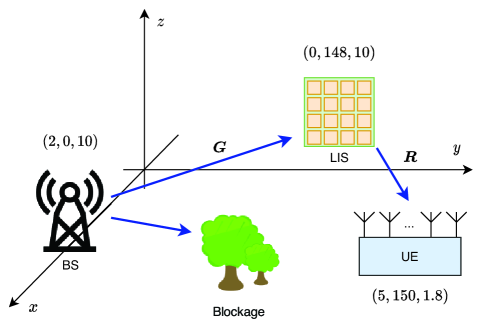
Figure 2: Simulation setup.

VI Simulation Results

In this section, we evaluate the performance of our proposed joint transceiver and LIS design method. The proposed method is based on the approximation of the truncated SVD of the effective (cascade) channel, and thus is referred to as Truncated-SVD-based beamforming (T-SVD-BF). In our simulations, we adopt a three-dimensional setup as shown in Fig. 2. The coordinates of the BS, the LIS and the UE are respectively given as $(x_{\rm BS},0,z_{\rm BS})$, $(0,y_{\rm LIS},z_{\rm LIS})$, and $(x_{\rm UE},y_{\rm UE},z_{\rm UE})$, where we set $x_{\rm BS}=2$m, $z_{\rm BS}=10$m, ${y}_{\rm LIS}=148$m, $z_{\rm LIS}=10$m, $x_{\rm UE}=5$m, $y_{\rm UE}=150$m, and $z_{\rm UE}=1.8$m. The distance between the BS (LIS) and the LIS (UE) can be easily calculated and given as $148$m ($9.8$m).

Slightly different from our previous definition, the effective channel is modeled as follows by considering the transmitter and receiver antenna gains [47]

$$\boldsymbol{H}_{\rm eff}=G_{t}G_{r}\boldsymbol{R}\boldsymbol{\Phi}\boldsymbol{G}$$ (48)

where $G_{t}$ and $G_{r}$ represent the transmitter and receiver antenna gains, respectively. The BS-LIS channel $\boldsymbol{G}$ and the LIS-UE channel $\boldsymbol{R}$ are modeled as follows

$$\boldsymbol{G}= \sqrt{\frac{N_{t}M}{P}}\bigg{(}\tilde{\alpha}_{1}\boldsymbol{a}_{R_{\rm LIS}}(\theta_{1}^{r},\eta_{1}^{r})\boldsymbol{a}_{T_{\rm BS}}^{H}(\gamma_{1}^{t})$$

$$+\sum_{i=2}^{P}\tilde{\alpha}_{i}\boldsymbol{a}_{R_{\rm LIS}}(\theta_{i}^{r},\eta_{i}^{r})\boldsymbol{a}_{T_{\rm BS}}^{H}(\gamma_{i}^{t})\bigg{)},$$ (49)

$$\boldsymbol{R}= \sqrt{\frac{MN_{r}}{L}}\bigg{(}\tilde{\beta}_{1}\boldsymbol{a}_{R_{\rm UE}}(\gamma_{1}^{r})\boldsymbol{a}_{T_{\rm LIS}}^{H}(\theta_{1}^{t},\eta_{1}^{t})$$

$$+\sum_{i=2}^{L}\tilde{\beta}_{i}\boldsymbol{a}_{R_{\rm UE}}(\gamma_{i}^{r})\boldsymbol{a}_{T_{\rm LIS}}^{H}(\theta_{i}^{t},\eta_{i}^{t})\bigg{)},$$ (50)

where $\tilde{\alpha}_{1}(\tilde{\beta}_{1})\sim{\cal CN}(0,10^{-0.1\kappa})$ denotes the complex gain of the LOS path, $\kappa$ is the path loss given by [37]

$$\kappa=a+10b\log_{10}(\tilde{d})+\xi$$ (51)

in which $\tilde{d}$ denotes the distance between the transmitter and the receiver, and $\xi\sim\mathcal{N}(0,\sigma_{\xi}^{2})$. The values of $a$, $b$ $\sigma_{\xi}$ are set to be $a=61.4$, $b=2$, and $\sigma_{\xi}=5.8$dB as suggested by LOS real-world channel measurements [37], $\tilde{\alpha}_{i}(\tilde{\beta_{i}})\sim\mathcal{CN}(0,10^{-0.1(\kappa+\mu)})$ stands for the complex gain of the associated NLOS path, and $\mu$ is the Rician factor [26, 48]. Unless specified otherwise, we assume that the LIS employs a UPA with $M=M_{y}\times M_{z}=16\times 16$, the BS and the UE adopt ULAs with $N_{t}=N_{r}=64$. Other parameters are set as follows: $R_{t}=R_{r}=6$, $N_{s}=4$, $L=P=7$, $\mu=10$, $G_{t}=24.5$dBi, $G_{r}=0$dBi. The carrier frequency is set to $28$GHz, the bandwidth is set to $251.1886$MHz and thus the noise power is $\sigma^{2}=-174+10\log_{10}B=-90$dBm.

We compare our proposed method with the following three state-of-the-art algorithms, namely, the sum-path-gain maximization (SPGM) method which aims to maximize the Frobenius-norm of the effective channel $\boldsymbol{H}_{\text{eff}}$ [24], the AO-based algorithm [25], and the WMMSE-based algorithm [27]. Note that the WMMSE-based method is designed for multicell-multiuser scenarios. But it can easily adapted to the point-to-point scenario considered in this paper.

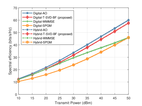
Figure 3: Spectral efficiency versus transmit power $\rho$.

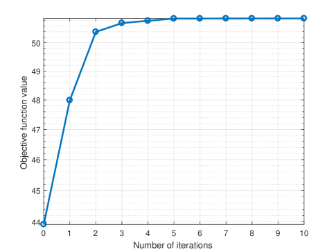
Figure 4: Convergence behavior of the proposed algorithm for solving (23)

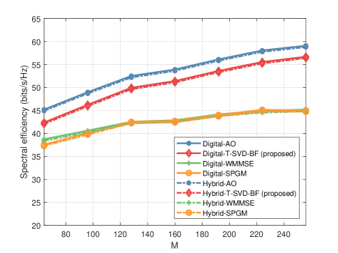
(a) Spectral efficiency versus the number of LIS elements $M$.

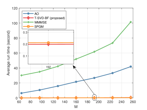
(b) Average run time versus the number of LIS elements $M$.

Figure 5: Spectral efficiency and average run time versus number of LIS elements, $M$.

VI-A Perfect Channel State Information

In this section, we assume perfect channel state information (CSI) is available at the BS. In Fig. 3, we plot the spectral efficiency of respective algorithms versus the transmit power $\rho$, where “digital” and “hybrid” respectively represent the spectral efficiency achieved by fully digital precoding/combining matrices and hybrid precoding/combining matrices. Here hybrid precoding/combining matrices are obtained via the manifold optimization-based method developed in Section IV. We observe that for all four algorithms, the performance of hybrid precoding/combining is very close to that of fully digital precoding/combining, which corroborates the claim that hybrid beamforming/combining with a small number of RF chains can asymptotically approach the performance of fully digital beamforming/combining for a sufficiently large number of transceiver antennas. In addition, we see that our proposed method T-SVD-BF presents a clear performance advantage over the SPGM method and the WMMSE-based method. Particularly, the substantial improvement over the SPGM can be attributed to the fact that our proposed method yields a well-conditioned effective channel matrix with a smaller condition number, thus creating a more amiable propagation environment for data transmission. We also note that our proposed method achieves performance close to the AO-based method. The convergence behavior of our proposed manifold-based algorithm used to solve the passive beamforming design problem (23) is depicted in Fig. 4, where we set $\rho=30$dBm. It can be seen that the proposed manifold-based algorithm has a relatively fast convergence rate and attains the maximum objective function value within only ten iterations.

Fig. 5 depicts the spectral efficiency and average run time of respective algorithms versus the number of LIS elements, where the transmit power $\rho$ is set to $50$dBm, and to vary $M$, we fix $M_{y}=16$ and increase $M_{z}$. All algorithms are executed on a 2.90GHz Intel Core i7 PC with 64GB RAM. We see that for all four algorithms, the spectral efficiency increases as the number of passive elements increases. For this setup, the SPGM and the WMMSE methods achieve similar performance. Our proposed method outperforms the SPGM and the WMMSE by a big margin, and the performance gap becomes more pronounced as $M$ increases. It is also observed that the spectral efficiency of our proposed method is slightly lower (by about $4\%$ spectral efficiency loss) than that of the AO-based method. Nevertheless, our proposed method is much more computationally efficient than the AO-based method, as reported in Fig. 5 (b). For instance, the average run time required by our proposed method T-SVD-BF is $0.1988$ second when $M=192$, while it takes the AO-based method about $26.7357$ seconds to yield a satisfactory solution. Such a substantial complexity reduction makes our proposed method a more practical choice for LIS-assisted mmWave communications where a large number of antennas as well as a large number of reflecting elements are likely to be employed to compensate the severe path loss. In addition, it is observed that our proposed method outperforms the WMMSE-based method in terms of both spectral efficiency and computational complexity.

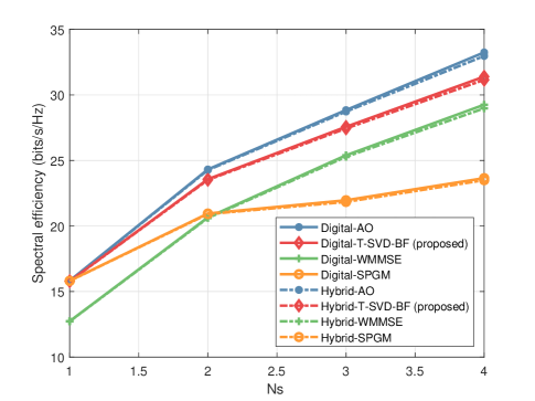
Figure 6: Spectral efficiency versus the number of data streams $N_{s}$.

In Fig. 6, we plot the spectral efficiency versus the number of data streams, where the transmit power $\rho$ is set to $30$dBm and the number of passive elements is set to $M=256$. It is observed that the spectral efficiency of T-SVD-BF, AO and WMMSE improves rapidly as $N_{s}$ increases, while the performance improvement of SPGM is quite limited. Again, we observe that T-SVD-BF achieves a substantial computational complexity reduction, at the expense of mild performance degradation compared to the AO-based method. The average run time of our proposed method is $0.5637$ second when $N_{s}=3$, while it takes the AO-based method about $35$ seconds.

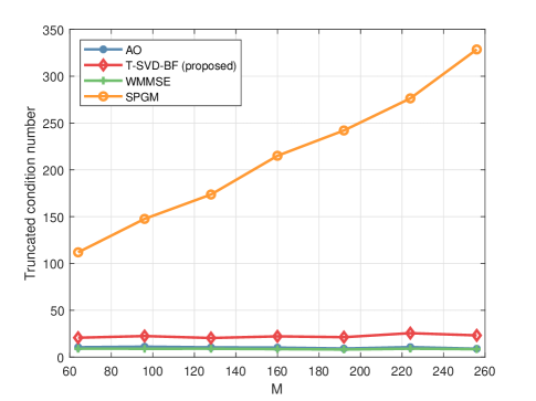
Figure 7: Truncated condition number versus the number of LIS elements $M$.

To gain an insight into how the LIS helps realize a favorable propagation environment, we use the truncated condition number as a metric to evaluate the capability of respective algorithms in reconfiguring the wireless channel. As is well known, the channel matrix condition number is regarded as an auxiliary metric for measuring how favorable the channel is. The truncated condition number is defined as $\frac{\boldsymbol{\Sigma}_{1}^{2}(1,1)}{\boldsymbol{\Sigma}^{2}_{1}(N_{s},N_{s})}$, where $\boldsymbol{\Sigma}_{1}(i,i)$ denotes the $i$th largest singular value of the effective channel $\boldsymbol{H}_{\text{eff}}$. Fig. 7 shows the truncated condition number versus the number of passive reflection elements. We observe that the truncated condition number of SPGM grows as $M$ increases, whereas the truncated condition numbers of the proposed method and the AO-based method are small and remain almost unchanged with an increasing $M$. This result indicates that our proposed method and the AO-based method are superior to SPGM in building a more favorable wireless channel. It also explains why SPGM does not gain much with the increase of the number of passive elements. An interesting observation is that the WMMSE-based method performs worse than our proposed method, despite of the fact that it has a smaller truncated condition number. The reason lies in that although the WMMSE-based method obtains more balanced singular values, the singular values are generally smaller (in terms of magnitude) than those singular values obtained by our proposed method, which prevents the WMMSE method from achieving a higher spectral efficiency.

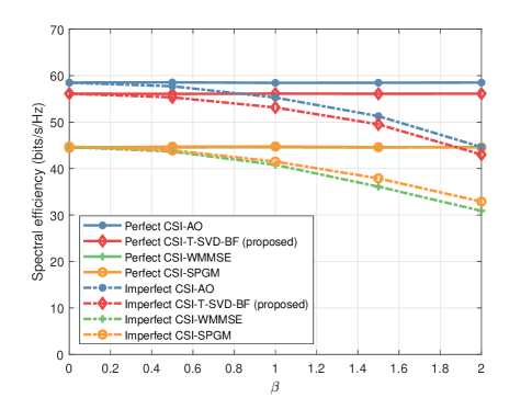
Figure 8: Spectral efficiency versus the estimation error $\beta$.

VI-B Imperfect Channel State Information

In practice, due to channel estimation errors, perfect knowledge of channel state information (CSI) is usually unavailable. It is therefore important to evaluate the performance of respective algorithms with inaccurate knowledge of AoAs and AoDs. To this end, let $\delta\triangleq\theta-\hat{\theta}$ denote the estimation error of the AoA/AOD parameter, where $\theta$ denotes the true AoA (AoD) and $\hat{\theta}$ is the estimated AoA (AoD). Note that our channel model consists of a set of AoA/AoD parameters, and we assume that the estimation errors for these AoA/AoD parameter are modeled as independent and identically distributed (i.i.d.) random variables following a same uniform distribution [49]:

$$f(\delta)=\left\{\begin{array}[]{ll}\frac{1}{2\beta},&\text{ if }-\beta\leq\delta\leq\beta\\ 0,&\text{ otherwise }\end{array}\right.$$ (54)

In our simulations, we set $N_{t}=N_{r}=64$, $M=M_{y}\times M_{z}=16\times 16=256$, $L=P=7$, and $\rho=50$dBm. Fig. 8 depicts the spectral efficiency versus the estimation error $\beta$, where $\beta$ varies from 0 to $2^{\circ}$, as suggested in [49]. We see that our proposed method behaves similarly as the AO-based method: both methods suffer nearly a same amount of performance loss as the estimation error increases. This result indicates that our proposed method does not exhibit higher sensitivity to inaccurate CSI than other methods. Moreover, it can be observed that our proposed method still presents a clear performance advantage over the SPGM and the WMMSE-based methods in the presence of channel estimation errors.

VII Conclusion

In this paper, we considered an LIS-assisted downlink mmWave MIMO system with hybrid precoding/combining. The objective is to maximize the spectral efficiency by jointly optimizing the passive beamforming matrix at the LIS and the hybrid precoder (combiner) at the BS (UE). To tackle this non-convex problem, we developed a manifold optimization (MO)-based algorithm by exploiting the inherent structure of the effective (cascade) mmWave channel. Simulation results showed that by carefully designing phase shift parameters at the LIS, our proposed method can help create a favorable propagation environment with a small channel matrix condition number. Besides, it can achieve a performance comparable to those of state-of-the-art algorithms, while at a much lower computational complexity.

References

- [1] T. S. Rappaport, J. N. Murdock, and F. Gutierrez, “State of the art in 60-GHz integrated circuits and systems for wireless communications,” Proc. IEEE, vol. 99, no. 8, pp. 1390–1436, Aug. 2011.
- [2] S. Rangan, T. S. Rappaport, and E. Erkip, “Millimeter-wave cellular wireless networks: Potentials and challenges,” Proc. IEEE, vol. 102, no. 3, pp. 366–385, Mar. 2014.
- [3] A. Ghosh, T. A. Thomas, M. C. Cudak, R. Ratasuk, P. Moorut, F. W. Vook, T. S. Rappaport, G. R. MacCartney, S. Sun, and S. Nie, “Millimeter-wave enhanced local area systems: A high-data-rate approach for future wireless networks,” IEEE J. Sel. Areas Commun., vol. 32, no. 6, pp. 1152–1163, Jun. 2014.
- [4] S. Sun, T. S. Rappaport, M. Shafi, P. Tang, J. Zhang, and P. J. Smith, “Propagation models and performance evaluation for 5G millimeter-wave bands,” IEEE Trans. Veh. Technol., vol. 67, no. 9, pp. 8422–8439, Sep. 2018.
- [5] A. Alkhateeb, J. Mo, N. Gonzalez-Prelcic, and R. Heath, “MIMO precoding and combining solutions for millimeter-wave systems,” IEEE Commun. Mag., vol. 52, no. 12, pp. 122–131, Dec. 2014.
- [6] A. L. Swindlehurst, E. Ayanoglu, P. Heydari, and F. Capolino, “Millimeter-wave massive MIMO: The next wireless revolution?” IEEE Commun. Mag., vol. 52, no. 9, pp. 56–62, Sep. 2014.
- [7] O. Abari, D. Bharadia, A. Duffield, and D. Katabi, “Enabling high-quality untethered virtual reality,” in 14th USENIX Symp. Netw. Syst. Des. and Implementation (NSDI 17). Boston, MA: USENIX Association, Mar. 27-29, 2017, pp. 531–544.
- [8] G. R. MacCartney, T. S. Rappaport, and S. Rangan, “Rapid fading due to human blockage in pedestrian crowds at 5G millimeter-wave frequencies,” in GLOBECOM 2017-2017 IEEE Global Commun. Conf. IEEE, 2017, pp. 1–7.
- [9] P. Wang, J. Fang, X. Yuan, Z. Chen, H. Duan, and H. Li, “Intelligent reflecting surface-assisted millimeter wave communications: Joint active and passive precoding design,” 2019, [Online]. Available: https://arxiv.org/abs/1908.10734.
- [10] X. Tan, Z. Sun, D. Koutsonikolas, and J. M. Jornet, “Enabling indoor mobile millimeter-wave networks based on smart reflect-arrays,” in IEEE Int. Conf. Comput. Commun. (INFOCOM), Honolulu, Hawaii, Apr. 15-19 2018, pp. 270–278.
- [11] N. S. Perović, M. Di Renzo, and M. F. Flanagan, “Channel capacity optimization using reconfigurable intelligent surfaces in indoor mmwave environments,” in ICC 2020-2020 IEEE Int. Conf. Commun. (ICC). IEEE, 2020, pp. 1–7.
- [12] X. Yang, C.-K. Wen, and S. Jin, “MIMO detection for reconfigurable intelligent surface-assisted millimeter wave systems,” IEEE J. Sel. Areas Commun., 2020.
- [13] C. Liaskos, S. Nie, A. Tsioliaridou, A. Pitsillides, S. Ioannidis, and I. Akyildiz, “A new wireless communication paradigm through software-controlled metasurfaces,” IEEE Commun. Mag., vol. 56, no. 9, pp. 162–169, Sep. 2018.
- [14] Y.-C. Liang, R. Long, Q. Zhang, J. Chen, H. V. Cheng, and H. Guo, “Large intelligent surface/antennas (LISA): Making reflective radios smart,” J. Commun. Inf. Netw., vol. 4, no. 2, pp. 40–50, 2019.
- [15] S. Hu, F. Rusek, and O. Edfors, “Beyond massive MIMO: The potential of data transmission with large intelligent surfaces,” IEEE Trans. Signal Process., vol. 66, no. 10, pp. 2746–2758, 2018.
- [16] E. Basar, M. Di Renzo, J. De Rosny, M. Debbah, M.-S. Alouini, and R. Zhang, “Wireless communications through reconfigurable intelligent surfaces,” IEEE Access, vol. 7, pp. 116 753–116 773, 2019.
- [17] Q. Wu and R. Zhang, “Towards smart and reconfigurable environment: Intelligent reflecting surface aided wireless network,” IEEE Commun. Mag., vol. 58, no. 1, pp. 106–112, 2020.
- [18] Y. Han, W. Tang, S. Jin, C.-K. Wen, and X. Ma, “Large intelligent surface-assisted wireless communication exploiting statistical CSI,” IEEE Trans. Veh. Technol., vol. 68, no. 8, pp. 8238–8242, 2019.
- [19] Q. Wu and R. Zhang, “Intelligent reflecting surface enhanced wireless network: Joint active and passive beamforming design,” in 2018 IEEE Global Commun. Conf. (GLOBECOM), Abu Dhabi, UAE, Dec. 10-12 2018, pp. 1–6.
- [20] C. Huang, A. Zappone, G. C. Alexandropoulos, M. Debbah, and C. Yuen, “Reconfigurable intelligent surfaces for energy efficiency in wireless communication,” IEEE Trans. Wireless Commun., vol. 18, no. 8, pp. 4157–4170, Aug. 2019.
- [21] Q. Wu and R. Zhang, “Intelligent reflecting surface enhanced wireless network via joint active and passive beamforming,” IEEE Trans. Wireless Commun., vol. 18, no. 11, pp. 5394–5409, Nov. 2019.
- [22] X. Li, J. Fang, F. Gao, and H. Li, “Joint active and passive beamforming for intelligent reflecting surface-assisted massive MIMO systems,” 2019, [Online]. Available: https://arxiv.org/abs/1912.00728.
- [23] M. Cui, G. Zhang, and R. Zhang, “Secure wireless communication via intelligent reflecting surface,” IEEE Wireless Commun. Lett., vol. 8, no. 5, pp. 1410–1414, 2019.
- [24] B. Ning, Z. Chen, W. Chen, and J. Fang, “Beamforming optimization for intelligent reflecting surface assisted MIMO: A sum-path-gain maximization approach,” IEEE Wireless Commun. Lett., vol. 9, no. 7, pp. 1105–1109, 2020.
- [25] S. Zhang and R. Zhang, “Capacity characterization for intelligent reflecting surface aided MIMO communication,” IEEE J. Sel. Areas Commun., 2020.
- [26] K. Ying, Z. Gao, S. Lyu, Y. Wu, H. Wang, and M. Alouini, “GMD-based hybrid beamforming for large reconfigurable intelligent surface assisted millimeter-wave massive MIMO,” IEEE Access, vol. 8, pp. 19 530–19 539, 2020.
- [27] C. Pan, H. Ren, K. Wang, W. Xu, M. Elkashlan, A. Nallanathan, and L. Hanzo, “Multicell MIMO communications relying on intelligent reflecting surface,” IEEE Trans. Wireless Commun., 2020.
- [28] C. Pan, H. Ren, K. Wang, M. Elkashlan, A. Nallanathan, J. Wang, and L. Hanzo, “Intelligent reflecting surface aided MIMO broadcasting for simultaneous wireless information and power transfer.” IEEE J. Sel. Areas Commun., 2020.
- [29] D. Mishra and H. Johansson, “Channel estimation and low-complexity beamforming design for passive intelligent surface assisted MISO wireless energy transfer,” in 2019 IEEE Int. Conf. Acoust. Speech and Signal Process. (ICASSP), May 2019, pp. 4659–4663.
- [30] P. Wang, J. Fang, H. Duan, and H. Li, “Compressed channel estimation and joint beamforming for intelligent reflecting surface-assisted millimeter wave systems,” IEEE Signal Process. Lett., vol. 27, pp. 905–909, 2020.
- [31] J. Chen, Y.-C. Liang, H. V. Cheng, and W. Yu, “Channel estimation for reconfigurable intelligent surface aided multi-user MIMO systems,” 2019 [Online]. Available: https://arxiv.org/abs/1912.03619.
- [32] T. Lin, X. Yu, Y. Zhu, and R. Schober, “Channel estimation for intelligent reflecting surface-assisted millimeter wave MIMO systems,” 2020 [Online]. Available: https://arXiv.org/abs/2005.04720.
- [33] X. Yu, J.-C. Shen, J. Zhang, and K. B. Letaief, “Alternating minimization algorithms for hybrid precoding in millimeter wave MIMO systems,” IEEE J. Sel. Areas Commun., vol. 10, no. 3, pp. 485–500, 2016.
- [34] H. Sawada, Y. Shoji, C. Choi, K. Sato, R. Funada, S. Kato, M. Umehira, and H. Ogawa, “LOS office channel model based on TSV model,” IEEE 802. 15-06-0377-02-003c, Sep., 2006.
- [35] O. E. Ayach, S. Rajagopal, S. Abu-Surra, Z. Pi, and R. W. Heath, “Spatially sparse precoding in millimeter wave MIMO systems,” IEEE Trans. Wireless Commun., vol. 13, no. 3, pp. 1499–1513, Mar. 2014.
- [36] X. Gao, L. Dai, S. Han, C.-L. I, and R. W. Heath, “Energy-efficient hybrid analog and digital precoding for mmwave MIMO systems with large antenna arrays,” IEEE J. Sel. Areas Commun., vol. 34, no. 4, pp. 998–1009, Apr. 2016.
- [37] M. R. Akdeniz, Y. Liu, M. K. Samimi, S. Sun, S. Rangan, T. S. Rappaport, and E. Erkip, “Millimeter wave channel modeling and cellular capacity evaluation,” IEEE J. Sel. Areas Commun., vol. 32, no. 6, pp. 1164–1179, Jun. 2014.
- [38] H. Kasai, “Fast optimization algorithm on complex oblique manifold for hybrid precoding in millimeter wave MIMO systems,” in 2018 IEEE Global Conf. Signal Info. Process. (GlobalSIP). IEEE, 2018, pp. 1266–1270.
- [39] T. L. Marzetta, Fundamentals of massive MIMO. Cambridge University Press, 2016.
- [40] J. Chen, “When does asymptotic orthogonality exist for very large arrays?” in 2013 IEEE Global Commun. Conf. (GLOBECOM), Atlanta, GA, Dec. 9-13 2013, pp. 4146–4150.
- [41] Q. Shi, M. Razaviyayn, Z.-Q. Luo, and C. He, “An iteratively weighted MMSE approach to distributed sum-utility maximization for a MIMO interfering broadcast channel,” IEEE Trans. Signal Process., vol. 59, no. 9, pp. 4331–4340, 2011.
- [42] Q. Shi and M. Hong, “Spectral efficiency optimization for millimeter wave multiuser MIMO systems,” IEEE J. Sel. Topics Signal Process., vol. 12, no. 3, pp. 455–468, 2018.
- [43] K. Alhujaili, V. Monga, and M. Rangaswamy, “Transmit MIMO radar beampattern design via optimization on the complex circle manifold,” IEEE Trans. Signal Process., vol. 67, no. 13, pp. 3561–3575, 2019.
- [44] P.-A. Absil, R. Mahony, and R. Sepulchre, Optimization algorithms on matrix manifolds. Princeton University Press, 2009.
- [45] N. Boumal, B. Mishra, P.-A. Absil, and R. Sepulchre, “Manopt, a matlab toolbox for optimization on manifolds,” The Journal Mach. Learn. Res., vol. 15, no. 1, pp. 1455–1459, 2014.
- [46] A. Oppenheim, “Inequalities connected with definite Hermitian forms, II,” The Amer. Math. Monthly, vol. 61, no. 7P1, pp. 463–466, 1954.
- [47] B. Ning, Z. Chen, W. Chen, Y. Du, and J. Fang, “Terahertz multi-user massive MIMO with intelligent reflecting surface: Beam training and hybrid beamforming,” 2019, [Online]. Available: https://arXiv.org/abs/1912.11662.
- [48] M. K. Samimi, G. R. MacCartney, S. Sun, and T. S. Rappaport, “28 GHz millimeter-wave ultrawideband small-scale fading models in wireless channels,” in 2016 IEEE 83rd Veh. Technol. Conf. (VTC Spring). IEEE, 2016, pp. 1–6.
- [49] C. Pradhan, A. Li, L. Zhuo, Y. Li, and B. Vucetic, “Beam misalignment aware hybrid transceiver design in mmwave MIMO systems,” IEEE Trans. Veh. Technol., vol. 68, no. 10, pp. 10 306–10 310, 2019.