Robust Fairness under Covariate Shift

Abstract

Making predictions that are fair with regard to protected attributes (race, gender, age, etc.) has become an important requirement for classification algorithms. Existing techniques derive a fair model from sampled labeled data relying on the assumption that training and testing data are identically and independently drawn (iid) from the same distribution. In practice, distribution shift can and does occur between training and testing datasets as the characteristics of individuals interacting with the machine learning system change. We investigate fairness under covariate shift, a relaxation of the iid assumption in which the inputs or covariates change while the conditional label distribution remains the same. We seek fair decisions under these assumptions on target data with unknown labels. We propose an approach that obtains the predictor that is robust to the worst-case testing performance while satisfying target fairness requirements and matching statistical properties of the source data. We demonstrate the benefits of our approach on benchmark prediction tasks.

Introduction

Supervised learning algorithms typically focus on optimizing one singular objective: predictive performance on unseen data. However, the social impact of unwanted bias in these algorithms has become increasingly important. Machine learning systems that disadvantage specific groups are less likely to be accepted and may violate disparate impact law (Chang 2006; Kabakchieva 2013; Lohr 2013; Shipp et al. 2002; Obermeyer and Emanuel 2016; Moses and Chan 2014; Shaw and Gentry 1988; Carter and Catlett 1987; O’Neil 2016). Fairness through unawareness, which simply denies knowledge of protected group membership to the predictor, is insufficient to effectively guarantee fairness because other characteristics or covariates may correlate with protected group membership (Pedreshi, Ruggieri, and Turini 2008). Thus, there has been a surge of interest in the machine learning community to define fairness requirements reflecting desired behavior and to construct learning algorithms that more effectively seek to satisfy those requirements in various settings (Mehrabi et al. 2019; Barocas, Hardt, and Narayanan 2017; Calmon et al. 2017; Donini et al. 2018; Dwork et al. 2012, 2017; Hardt, Price, and Srebro 2016; Zafar et al. 2017a; Zemel et al. 2013; Jabbari et al. 2016; Chierichetti et al. 2017).

Though many definitions and measures of (un)fairness have been proposed (See Verma and Rubin (2018); Mehrabi et al. (2019)), the most widely adopted are group fairness measures of demographic parity (Calders, Kamiran, and Pechenizkiy 2009), equalized opportunity, and equalized odds (Hardt, Price, and Srebro 2016). Techniques have been developed as either post-processing steps (Hardt, Price, and Srebro 2016) or in-processing learning methods (Agarwal et al. 2018; Zafar et al. 2017a; Rezaei et al. 2020) seeking to achieve fairness according to these group fairness definitions. These methods attempt to make fair predictions at testing time by strongly assuming that training and testing data are independently and identically drawn (iid) from the same distribution, so that providing fairness on the training dataset provides approximate fairness on the testing dataset.

In practice, it is common for data distributions to shift between the training data set (source distribution) and the testing data set (target distribution). For example, the characteristics of loan applicants may differ significantly over time due to macroeconomic trends or changes in the self-selection criteria that potential applicants employ. Fairness methods that ignore such shifts may satisfy definitions for fairness on training samples, while violating those definitions severely on testing data. Indeed, disparate performance for underrepresented groups in computer vision tasks has been attributed to manually labeled data that is highly biased compared to testing data (Yang et al. 2020). Explicitly incorporating these shifts into the design of predictors is crucial for realizing fairer applications of machine learning in practice. However, the resulting problem setting is particularly challenging; access to labels is only available for the training distribution. Fair prediction methods could fail by using only source labels, especially for fairness definitions that condition on ground-truth labels, like equal opportunity.

Figure 1 illustrates the declining performance of a post-processing method (Hardt, Price, and Srebro 2016) and an in-processing method (Rezaei et al. 2020) that do not consider distribution shift and instead only depend on source fairness measurements. Therefore, relying on the iid assumption, which is often violated in practice, introduces significant limitations for realizing desired fairness in critical applications.

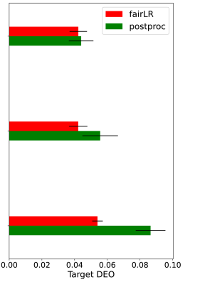
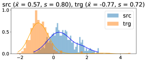
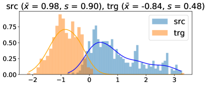
Figure 1: The difference of equalized opportunity between two genders in German UCI dataset evaluated on the target distribution for (a) the post-processing method of Hardt, Price, and Srebro (2016) and (b) an in-processing fairLR method (Rezaei et al. 2020), that both do not account for distribution shift, and correct true positive rate parity on source data. The histograms on the left show the corresponding distribution shift on first principal component of the covariates between source and target data. The shift intensity has an overall increasing effect on DEO violation of both methods. Experiment section includes details on sampling procedure.

We seek to address the task of providing fairness guarantees under the non-iid assumption of covariate shift. Covariate shift is a special case of data distribution shift. It assumes that the relationship between labels and covariates (inputs) is the same for both distributions, while only the source and target covariate distributions differ. Under the fair prediction setting, the sensitive group features are usually correlated with other features. Covariate shift then indicates that the labels given the covariates, including the sensitive group features, stays the same between two distributions. For example, even though there are fewer female loan applicants in area A than area B, which causes a marginal input distribution to shift between these two areas, we believe the probability of belonging to the advantages class (e.g., repaying a loan) given the full covariate should be the same.

In this paper, we propose a robust estimation approach for constructing a fair predictor under covariate shift. We summarize our contribution as follows: We formulate the fair prediction problem as a game between an adversary choosing conditional label distributions to fairly minimize predictive loss on the target distribution, and an adversary choosing conditional label distributions that maximize that same objective. Constraints on the adversary require it to match statistics under the source distribution. Fairness is incorporated into the formulation by a penalty term in the objective that evaluates the fairness on the target input distribution and adversary’s conditional label distribution. We derive a convex optimization problem from the formulation and obtain the predictor’s and adversary’s conditional label distribution that are parametric, but cannot be solved analytically. Based on the formulation, we propose a batch gradient descent algorithm for learning the parameters. We compare our proposed method with baselines that only account for covariate shift or fairness or both. We demonstrate that our method outperforms the baselines on both predictive performance and the fairness constraints satisfaction under covariate shift settings.

Related Work

Fairness

Various methods have been developed in recent years to achieve fair classification according to group fairness definitions. These techniques can be broadly categorized as pre-processing modifications to the input data or fair representation learning (Kamiran and Calders 2012; Calmon et al. 2017; Zemel et al. 2013; Feldman et al. 2015; Del Barrio et al. 2018; Donini et al. 2018; Guidotti et al. 2018), post-processing correction of classifiers’ outputs (Hardt, Price, and Srebro 2016; Pleiss et al. 2017), in-processing methods that incorporate the fairness constraints into the training process and parameter learning procedure (Donini et al. 2018; Zafar et al. 2017c, a, b; Cotter et al. 2018; Goel, Yaghini, and Faltings 2018; Woodworth et al. 2017; Kamishima, Akaho, and Sakuma 2011; Bechavod and Ligett 2017; Quadrianto and Sharmanska 2017; Rezaei et al. 2020), meta-algorithms (Celis et al. 2019; Menon and Williamson 2018), reduction-based methods (Agarwal et al. 2018; Cotter et al. 2018), or generative-adversarial training (Madras et al. 2018; Zhang, Lemoine, and Mitchell 2018; Celis and Keswani 2019; Xu et al. 2018; Adel et al. 2019).

The closest to our work in this category is the fair robust log-loss predictor of Rezaei et al. (2020), which operates under an iid assumption. That formulation similarly builds a minimax game between a predictor and worst-case approximator of the true distribution. The main difference is that under the iid assumption, the true/false positive rates of target groups can be expressed as a linear constraint on the source data, in which the ground truth label is known. However, in our work, no sample-based constraint is available for measuring true/false positive rates on target data, because the target true label is unknown under the covariate shift assumption. Thus, we enforce these fairness measures by an expected penalty of the worst-case approximation of the target data.

Covariate Shift

General distribution and domain shift works focus on the joint distribution shift between the training and testing datasets (Daume III and Marcu 2006; Ben-David et al. 2007; Blitzer et al. 2008). Particular assumptions like covariate shift (Shimodaira 2000; Sugiyama, Krauledat, and Müller 2007; Gretton et al. 2009) and label shift (Schölkopf et al. 2012; Lipton, Wang, and Smola 2018; Azizzadenesheli et al. 2019) help quantify the distribution shift using importance weights since they introduce invariance in conditional distributions between the training and testing. Importance weighting methods under covariate shift suffer from high variance and sensitivity to weight estimation methods. It has been shown to often be brittle—providing no finite sample generalization guarantees—even for seemingly benign amounts of shift (Cortes, Mansour, and Mohri 2010). Applying importance weighting to fair prediction has not been broadly investigated and may suffer from a similar issue.

Fairness under perturbation of the attribute has been studied by Awasthi, Kleindessner, and Morgenstern (2020). Lamy et al. (2019) study fair classification when the attribute is subjected to noise according to a mutually contaminated model (Scott, Blanchard, and Handy 2013). Our method works for a general shift on the joint distribution of attribute and features, and does not rely on a particular noise model.

Causal analysis has also been proposed for addressing fairness under dataset shift (Singh et al. 2019). It requires a known causal graph of the data generating process, with a context variable causing the shift, as well as the known separating set of features. Our model makes no assumptions about the underlying structure of the covariates. We assume covariate shift, which relates with causal models when there is no unobserved confounders between covariates and labels. Given a known separating set of features in the causal model under data shift, the covariate shift assumption holds if we use only the separating set of features for prediction. Our model builds on robust classification method of (Liu and Ziebart 2014) under covariate shift, where the target distribution is estimated by a worst-case adversary that maximizes the log-loss while matching the feature statistics under source distribution. Therefore, if we know the separating set of features, we can incorporate them as constraints for the adversary. However, it is usually difficult to know the exact causal model of the data generating process in practice.

Approach

Preliminaries & Notation

We assume a binary classification task $Y,\widehat{Y}\in\{0,1\}$, where $Y$ denotes the true label, and $\widehat{Y}$ denotes the prediction for a given instance with features $\mathbf{\bm{X}}\in\mathcal{X}$ and group attribute $A\in\{0,1\}$. We consider $y=1$ as the privileged class (e.g., an applicant who would repay a loan). Further, we assume a given source distribution $(\mathbf{\bm{X}},A,Y)\sim P_{\text{src}}$ over features, attribute, and label, and a target distribution $(\mathbf{\bm{X}},A)\sim P_{\text{trg}}$ over features and attribute only, throughout our paper.

Fairness Definitions

Our model seeks to satisfy the group fairness notions of equalized opportunity and odds (Hardt, Price, and Srebro 2016). Our focus in this paper is equalized opportunity, which requires equal true positive rates across groups, i.e., for a general probabilistic classifier $P$:

$$P(\widehat{Y}\!=\!1|A\!=\!1,Y\!=\!1) =P(\widehat{Y}\!=\!1|A\!=\!0,Y\!=\!1).$$ (1)

Our model can be generalized for equal odds, which in addition to providing equal true positive rates across groups, also requires equal false positive rates across groups:

$$P(\widehat{Y}\!=\!1|A\!=\!1,Y\!=\!0) =P(\widehat{Y}\!=\!1|A\!=\!0,Y\!=\!0).$$ (2)

For Demographic parity (Calders, Kamiran, and Pechenizkiy 2009) which requires equal positive rates across protected groups, i.e., $P(\widehat{Y}=1|A=1)=P(\widehat{Y}=1|A=0)$, our model reduces to a special case, as we later explain.

Covariate Shift

In the context of fair prediction, the covariate shift assumption is that the distribution of covariates and group membership can shift between source and target distributions:

$$P_{\text{src}}(\mathbf{\bm{x}},a,y)=P_{\text{src}}(\mathbf{\bm{x}},a)P(y|\mathbf{\bm{x}},a)$$ (3)

$$P_{\text{trg}}(\mathbf{\bm{x}},a,y)=P_{\text{trg}}(\mathbf{\bm{x}},a)P(y|\mathbf{\bm{x}},a).$$ (4)

Note that we do not assume how the sensitive group membership $a$ is correlated with other features $\mathbf{\bm{x}}$. If causal structure between the features and labels were known, as assumed in Singh et al. (2019), we could also incorporate a hidden or latent covariate shift assumption. For example, given that there is no unobserved confounder between the covariate and the labels, if $h=\Phi(\mathbf{\bm{x}},a)$ represents the separating set of features, we can assume $P_{\text{src}}(y|h=\Phi(\mathbf{\bm{x}},a))=P_{\text{trg}}(y|h=\Phi(\mathbf{\bm{x}},a))$ and use $\Phi(\mathbf{\bm{x}},a)$ instead of $(\mathbf{\bm{x}},a)$ in our formulation. In this paper, we still use $(\mathbf{\bm{x}},a)$ to represent the covariates for simplicity.

Importance Weighting

A standard approach for addressing covariate shift is to reweight the source data to represent the target distribution (Sugiyama, Krauledat, and Müller 2007). A desired statistic $f(x,a,y)$ of the target distribution can be obtained using samples from the source distribution $(x_{i},a_{i},y_{i})_{i=1:n}$:

$$\mathbb{E}_{\begin{subarray}{c}P_{\text{trg}}(\mathbf{\bm{x}},a)\\ P(y|\mathbf{\bm{x}},a)\end{subarray}}\!\!\left[f(\mathbf{\bm{X}},A,Y)\right]\approx\sum_{i=1}^{n}\frac{{P_{\text{trg}}}(\mathbf{\bm{x}}_{i},a_{i})}{P_{\text{src}}(\mathbf{\bm{x}}_{i},a_{i})}f(\mathbf{\bm{x}}_{i},a_{i},y_{i}).$$ (5)

As long as the source distribution has support for the entire target distribution (i.e., $P_{\text{trg}}(\mathbf{\bm{x}},a)>0\implies P_{\text{src}}(\mathbf{\bm{x}},a)>0$), this approximation is exact asymptotically as $n\rightarrow\infty$. However, the approximation is only guaranteed to have bounded error for finite $n$ if the source distribution’s support for target distribution samples is lower bounded (Cortes, Mansour, and Mohri 2010): $\mathbb{E}_{P_{\text{trg}}(\mathbf{\bm{x}},a)}\left[{P_{\text{trg}}(\mathbf{\bm{X}},A)}/{P_{\text{src}}(\mathbf{\bm{X}},A)}\right]<\infty$. Unfortunately, this requirement is fairly strict and will not be satisfied even under common and seemingly benign amounts of shift. For example, if source and target samples are drawn from Gaussian distributions with equal (co-)variance, but slightly different means, it is not satisfied.

Robust Log Loss Classification under Covaraite Shift

We base our method on the robust approach of Liu and Ziebart (2014) for covariate shift, which addresses this fragility of reweighting methods. In this formulation, the probabilistic predictor $\mathbb{P}$ minimizes the log loss on a worst-case approximation of the target distribution provided by an adversary $\mathbb{Q}$ that maximizes the log loss while matching the feature statistics of the source distribution:

$$\min_{\mathbb{P}(y|\mathbf{\bm{x}})\in\Delta}\;\max_{\mathbb{Q}(y|\mathbf{\bm{x}})\in\Delta\cap\Xi}\mathbb{E}_{P_{\text{trg}}(\mathbf{\bm{x}})\mathbb{Q}(y|\mathbf{\bm{x}})}[-\log\mathbb{P}(Y|\mathbf{\bm{X}})]$$

$$= \max_{\mathbb{P}(y|\mathbf{\bm{x}})\in\Delta\cap\Xi}H_{P_{\text{trg}}(\mathbf{\bm{x}})\mathbb{P}(y|\mathbf{\bm{x}})}(Y|\mathbf{\bm{X}}),$$ (6)

where a moment-matching constraint set $\Xi=\{\mathbb{Q}\,|\,\mathbb{E}_{P_{\text{src}}(\mathbf{\bm{x}})\mathbb{Q}(y|\mathbf{\bm{x}})}[\phi(\mathbf{\bm{X}},Y)]=\mathbb{E}_{P_{\text{src}}(\mathbf{\bm{x}},y)}[\phi(\mathbf{\bm{X}},Y)]\}$ on source data is enforced with $\phi(\mathbf{\bm{x}},y)$ denoting the feature function, and $\Delta$ denoting the conditional probability simplex. A first-order moments feature function, $\phi(\mathbf{x},y)=[x_{1}y,x_{2}y,\dots x_{m}y]^{\top}$, is typical but higher-order moments, e.g., $yx_{1},yx_{2}^{2},yx_{3}^{n},\dots$ or mixed moments, e.g., $yx_{1},yx_{1}x_{2},yx_{1}^{2}x_{2}x_{3},\dots$, can be included. The saddle point solution under these assumptions is $\mathbb{P}=\mathbb{Q}$ which reduces the formulation to maximizing the target distribution conditional entropy ($H$) while matching feature statistics of the source distribution. The probabilistic predictor of (Liu and Ziebart 2014) reduces to the following parametric form:

$$\mathbb{P}_{\theta}(y|\mathbf{\bm{x}})={e^{\frac{P_{\text{src}}(\mathbf{\bm{x}})}{P_{\text{trg}}(\mathbf{\bm{x}})}\theta^{\top}\phi(\mathbf{\bm{x}},y)}}\Big{/}{\sum_{y^{\prime}\in\mathcal{Y}}e^{\frac{P_{\text{src}}(\mathbf{\bm{x}})}{P_{\text{trg}}(\mathbf{\bm{x}})}\theta^{\top}\phi(\mathbf{\bm{x}},y^{\prime})}},$$ (7)

where the Lagrange multipliers $\theta$ maximize the target distribution log likelihood in the dual optimization problem.

Robust Log Loss for Fair Classification (IID)

The same robust log loss approach has been employed by Rezaei et al. (2020) for fair classification under the iid assumption ($P_{\text{trg}}=P_{\text{src}}$), where both the optimization objective and the constraints are evaluated on the source data. Since the true label is available during training, fairness can be enforced as a set of linear constraints on predictor $\mathbb{P}$, which yields a parametric dual form.

In contrast, under the non-iid assumption, the desired fairness on target cannot be directly inferred by enforcing constraints on the source. Additionally, the true/false positive rate parity constraints are no longer linear because the ground truth label on target data is unobserved. Thus, we replace the target label by a random variable distributed according to the worst-case approximation $\mathbb{Q}$, and seek fairness on target by augmenting the objective in (6) with an expected fairness penalty incurred by the worst-case target approximator $\mathbb{Q}$. In our formulation, the saddle point solution is no longer simple (i.e., $\mathbb{P}\neq\mathbb{Q}$), and no parametric form solution is available.

Formulation

Our formulation seeks a robust and fair predictor under the covariate shift assumption by playing a minimax game between a minimizing predictor and a worst-case approximator of the target distribution that matches the feature statistics from the source and marginals of the groups from target. We assume the availability of a set of labeled examples $\{\mathbf{\bm{x}}_{i},a_{i},y_{i}\}^{n}_{i=1}$ sampled from the source $P_{\text{src}}(\mathbf{\bm{x}},a,y)$ and unlabeled examples $\{\mathbf{\bm{x}}_{i},a_{i}\}^{m}_{i=1}$ sampled from target distribution $P_{\text{trg}}(\mathbf{\bm{x}},a)$ during training.

Definition 1.

The Fair Robust Log-Loss Predictor under Covariate Shift, $\mathbb{P}$ minimizes the worst-case expected log loss with an $\mu$-weighted expected fairness penalty on target, approximated by adversary $\mathbb{Q}$ constrained to match source distribution statistics (denoted by set $\Xi$) and group marginals on target ($\Gamma$):

$$\min_{\mathbb{P}\in\Delta}\;\max_{\mathbb{Q}\in\Delta\cap\Xi\cap\Gamma} \mathbb{E}_{P_{\text{trg}}(\mathbf{\bm{x}},a)\mathbb{Q}(y|\mathbf{\bm{x}},a)}[-\log\mathbb{P}(Y|\mathbf{\bm{X}},A)]$$ (8)

$$+ \mu\,\mathbb{E}_{P_{\text{trg}}(\mathbf{\bm{x}},a)\mathbb{Q}(y^{\prime}|\mathbf{\bm{x}},a)\mathbb{P}(y|\mathbf{\bm{x}},a)}[f(A,Y^{\prime},Y)]$$

such that:

$$\Xi(\mathbb{Q}):\mathbb{E}_{\begin{subarray}{c}P_{\text{src}}(\mathbf{\bm{x}},a)\\ \mathbb{Q}(y|\mathbf{\bm{x}},a)\end{subarray}}[\phi(\mathbf{\bm{X}},Y)]=\mathbb{E}_{P_{\text{src}}(\mathbf{\bm{x}},a,y)}[\phi(\mathbf{\bm{X}},Y)]\text{ and}$$

$$\Gamma(\mathbb{Q}):\mathbb{E}_{\begin{subarray}{c}P_{\text{trg}}(\mathbf{\bm{x}},a)\\ \mathbb{Q}(y|\mathbf{\bm{x}},a)\end{subarray}}[g_{k}(A,Y)]=\underbrace{\mathbb{E}_{\begin{subarray}{c}P_{\text{trg}}(\mathbf{\bm{x}},a)\\ \widetilde{P}_{\text{trg}}(y|\mathbf{\bm{x}},a)\end{subarray}}[g_{k}(A,Y)]}_{\widetilde{g}_{k}},$$

$\forall k\in\{0,1\}$, where $\phi$ is the feature function, $\mu$ is the fairness penalty weight, $g_{k}(.,.)$ is a selector function for group $k$ according to the fairness definition, i.e., for equalized opportunity: $g_{k}(A,Y)=\mathbb{I}(A\!=\!k\wedge Y\!=\!1)$ , $\widetilde{g}_{k}$ the estimated group density on target, and $f(.,.,.)$ is a weighting function of the mean score difference between the two groups:

$$f(A,Y,\widehat{Y})=\begin{cases}\frac{1}{\widetilde{g}_{1}}&\text{if }g_{1}(A,Y)\wedge\mathbb{I}(\widehat{Y}\!=\!1)\\ -\frac{1}{\widetilde{g}_{0}}&\text{if }g_{0}(A,Y)\wedge\mathbb{I}(\widehat{Y}\!=\!1)\\ 0&\text{otherwise.}\end{cases}$$ (9)

The $\Gamma$ constraint enforces $\mathbb{Q}$ to be consistent with the marginal probability of the groups on target ($\widetilde{g}_{k}$) for equalized opportunity (and odds). This marginal probability is unknown, since the true label $Y$ on target is unavailable. Thus, we estimate these marginal probabilities by employing the robust model (7) as $\widetilde{P}_{\text{trg}}(y|\mathbf{\bm{x}},a)$ in $\Gamma$ in (8) to first guess the labels under covariate shift ignoring fairness ($\mu=0$). We penalize the expected difference in true (or false) positive rate of groups in target according to our worst-case approximation of each example being positively labeled. This needs to be measured on the entire target example set and requires batch gradient updates to enforce.

Our formulation is flexible for all three mentioned definitions of group fairness. For equalized odds, a second penalty term for false positive rates ($g_{k}(A,Y)=\mathbb{I}(A=k\wedge Y=0)$) is required and the corresponding marginal matching constraint in $\Gamma$ needs to be added. For demographic parity ($g_{k}(A,Y)=\mathbb{I}(A=k)$), because the group definition is independent of the true label, the target groups are fully known and the fairness penalty reduces to a linear constraint of $\mathbb{P}$ on target. In this special case, there is no need for the $\Gamma$ constraint and $\mu$ can be treated as a dual variable for the linear fairness constraint. This reduces to the truncated logistic classifier of (Rezaei et al. 2020) with the exception that the fairness constraint is formed on the target data.

We obtain the following solution for the predictor $\mathbb{P}$ by leveraging strong minimax duality (Topsøe 1979; Grünwald and Dawid 2004) and strong Lagrangian duality (Boyd and Vandenberghe 2004).

Theorem 1.

Given binary class labels and protected attributes $y,a\in\{0,1\}$, the fair probabilistic classifier for equalized opportunity robust under covariate shift as defined in (8) can be obtained by solving:

$$\log\frac{1-\mathbb{P}(y=1|\mathbf{\bm{x}},a)}{\mathbb{P}(y=1|\mathbf{\bm{x}},a)}+\mu\,\mathbb{E}_{\mathbb{P}(y^{\prime}|\mathbf{\bm{x}},a)}\left[f(a,y=1,Y^{\prime})\right]$$

$$\quad+\frac{P_{\text{src}}(\mathbf{\bm{x}},a)}{P_{\text{trg}}(\mathbf{\bm{x}},a)}\theta^{\mathrm{T}}\left(\phi(\mathbf{\bm{x}},y=1)-\phi(\mathbf{\bm{x}},y=0)\right)$$ (10)

$$\quad+\!\sum_{k\in\{0,1\}}\lambda_{k}g_{k}(a,y=1)=0,$$

where $\theta$ and $\lambda$ are the dual Lagrange multipliers for source feature matching constraints ($\Xi$) and target group marginal matching ($\Gamma$) respectively, and $\mu$ is the penalty weight chosen to minimize the expected fairness violation on target.

Given the solution $\mathbb{P}^{*}$ obtained above, for $\mathbb{Q}$ to be in equilibrium (given $\theta$ and $\lambda$) it suffices to choose $\mathbb{Q}$ for $y=1$ such that: $\mathbb{Q}(y|\mathbf{\bm{x}},a)=$

$$\frac{\mathbb{P}^{*}(y|\mathbf{\bm{x}},a)}{1-\mu f(a,y,y)\mathbb{P}^{*}(y|\mathbf{\bm{x}},a)+\mu f(a,y,y)\mathbb{P}^{*^{2}}(y|\mathbf{\bm{x}},a)},$$ (11)

where additionally it must hold that $0\leq\mathbb{Q}(y|x,a)\leq 1:$

$$\implies\begin{cases}0<\mathbb{P}(y=1|\mathbf{\bm{x}},a)\leq\frac{1}{\mu f(a,1,1)}&\text{if }\mu f(a,1,1)>1\\ 0<\mathbb{P}(y=1|\mathbf{\bm{x}},a)<1&\text{ otherwise.}\end{cases}$$

Due to monotonicity, $\mathbb{P}$ in (10) is efficiently found using a binary-search in the simplex. For proofs and further details, we refer the interested reader to the appendix.

Enforcing fairness

Our model penalizes the expected fairness violation on the target approximated by worst-case adversary ($\mathbb{Q}$). We seek optimal penalty weight $\mu$ by finding the zero-point of expected fairness violation, i.e., $\mathbb{E}_{P_{\text{trg}}(\mathbf{\bm{x}},a)\mathbb{Q}(y^{\prime}|\mathbf{\bm{x}},a)\mathbb{P}(y|\mathbf{\bm{x}},a)}[f(A,Y^{\prime},Y)]$ on target (see (10)). Under the mild assumption that $\mathbb{Q}$ is sufficiently constrained by source feature constraints and target group marginal constraints, the approximated fairness violation by $\mathbb{Q}$ is monotone in the proximity of the zero point. Thus, we can find the exact zero point by a binary-search in a neighborhood around the zero point.

Learning

For a given fairness penalty weight $\mu$, our model seeks to learn the dual parameters $\theta$ and $\lambda$, such that the worst-case target approximator ($\mathbb{Q}_{\theta,\mu}$) matches the sample feature statistic from the source distribution and the marginal of groups on the target set. Given $\theta^{*},\lambda^{*}$ the solution of (10) obtains the optimal fair predictor $\mathbb{P}^{*}_{\theta^{*},\mu^{*}}$ which is robust against the covariate shift.

We employ L2 regularization on parameters $\theta$ to improve our model’s generalization. This corresponds to relaxing our feature matching constraints by a convex norm. We employ a batch gradient-only optimization to learn our model parameters. We perform a joint gradient optimization that updates the gradient of $\theta$ (which requires true label) from the source data and $\lambda$ (which does not require true label) from the target batch at each step. Note that we find the solution to the dual objective of (8) by gradient-only optimization without requiring the explicit calculation of the objective on the target dataset. Hence we only use the density ratios when calculating (10). The gradient optimization converges to the global optimum because the dual objective is convex in $\theta$ and $\lambda$.

Given an optimal $\mathbb{Q}^{*}$ from (11), a set of labeled source samples $\widetilde{P}_{\text{src}}(\mathbf{\bm{x}},a,y)$ and unlabeled target samples $\widetilde{P}_{\text{trg}}(\mathbf{\bm{x}},a)$, the gradient of our model parameters is calculated as follows:

$${\nabla}_{\theta}\mathcal{L}^{\text{trg}}(\mathbb{P},\mathbb{Q},\theta,\lambda)=\mathbb{E}_{\begin{subarray}{c}\widetilde{P}_{\text{src}}(\mathbf{\bm{x}},y)\\ \mathbb{Q}(\widehat{y}|\mathbf{\bm{x}},a)\end{subarray}}\phi(\mathbf{\bm{X}},\widehat{Y})-\mathbb{E}_{\widetilde{P}_{\text{src}}(\mathbf{\bm{x}},a,y)}\phi(\mathbf{\bm{X}},Y)$$

$${\nabla}_{\lambda_{a^{\prime}}}\mathcal{L}^{\text{trg}}(\mathbb{P},\mathbb{Q},\theta,\lambda)=\mathbb{E}_{\begin{subarray}{c}\widetilde{P}_{\text{trg}}(\mathbf{\bm{x}},a)\\ \mathbb{Q}(y|\mathbf{\bm{x}},a)\end{subarray}}[g_{k}(A,Y)]-\widetilde{g}_{k}.$$ (12)

Note that although the gradient of $\theta$ can be updated stochastically, the gradient update for $\lambda$ relies on calculating the $\mathbb{Q}$ marginal for each group on the target batch. This process is described in detail in Algorithm 1.

Input: Datasets $D_{\text{src}}=\{\mathbf{\bm{x}}_{i},a_{i},y_{i}\}^{n}_{i=1}$, $D_{\text{trg}}=\{\mathbf{\bm{x}}_{i},a_{i}\}^{m}_{i=1}$, ratios $\frac{P_{\text{src}}}{P_{\text{trg}}}$, feature function $\phi(\mathbf{\bm{x}},y)$, decaying learning rate $\eta_{t}$

Output: $\theta^{*},\lambda^{*}$

1 $\theta\leftarrow$ random initialization ;

2 $\lambda_{a}\leftarrow 0$ ;

3 repeat

4       Compute $\mathbb{P},\mathbb{Q}$ for all source dataset examples by finding solution to (10) and (11)

5      $\nabla_{\theta}\mathcal{L}\leftarrow\frac{1}{n}\sum_{i=1}^{n}\phi(\mathbf{\bm{x}}_{i},y_{i})-\frac{1}{n}\sum_{i=1}^{n}\sum_{y\in\mathcal{Y}}\mathbb{Q}(y|\mathbf{\bm{x}}_{i},a)\phi(\mathbf{\bm{x}}_{i},y)$ ;

6      

7      $\nabla_{\lambda_{k}}\mathcal{L}\leftarrow\widetilde{g}_{k}-\frac{1}{m}\sum_{i=1}^{m}\sum_{y\in\mathcal{Y}}\mathbb{Q}(y|\mathbf{\bm{x}},a)g_{k}(a,y)$ ;

8      

9      $\theta\leftarrow\eta_{t}(\nabla_{\theta}\mathcal{L}+C\nabla\|\theta\|)$

10      $\lambda\leftarrow\eta_{t}(\nabla_{\lambda}\mathcal{L})$ ;

11      

12until convergence;

Algorithm 1 Batch gradient update for Fair Robust Log-Loss learning under Covariate Shift

Experiments

We demonstrate the effectiveness of our method on biased samplings from four benchmark datasets:

• The COMPAS criminal recidivism risk assessment dataset (Larson et al. 2016). The task is to predict recidivism of a defendant based on criminal history.

• UCI German dataset (Dheeru and Karra Taniskidou 2017). The task it to classify good and bad credit according to personal information and credit history.

• UCI Drug dataset (Fehrman et al. 2017). The task is to classify type of drug consumer by personality and demongraphics.

• UCI Arrhythmia dataset (Dheeru and Karra Taniskidou 2017). The task is to distinguish between the presence and absence of cardiac arrhythmia.

Table 1 summarizes the statistics of each dataset.

Biased Sampling:

We model a general shift in the distribution of covariates between source and target, i.e., $P_{\text{src}}(\mathbf{\bm{x}},a)\neq P_{\text{trg}}(\mathbf{\bm{x}},a)$, by creating biased sampling based on the principal components of the covariates. We follow the previous literature on covariate shift (Gretton et al. 2009) and take the following steps to create the covariate shift on each dataset: We normalized all non-categorical features by z-score. We retrieve the first principal component $\mathcal{C}$ of covariates $(\mathbf{\bm{x}},a)$ by applying principal component analysis (PCA). We then estimate the mean $\mu(\mathcal{C})$ and standard deviation $\sigma(\mathcal{C})$, and set a Gaussian distribution $D_{t}(\mu(\mathcal{C}),\sigma(\mathcal{C}))$ for random sampling of target. We choose parameters $\alpha,\beta$ and set another Gaussian distribution $D_{s}(\mu(\mathcal{C})+\alpha,\frac{\sigma(\mathcal{C})}{\beta})$ for random sampling of source data. We fix the sample size for both source and target to $40\%$ of the original dataset; and construct the source data by sampling without replacement in proportion to $D_{s}$, and the target data by sampling without replacement from the remaining data in proportion to $D_{t}$.

Dataset	$n$	Features	Attribute
COMPAS	6,167	10	Race
German	1,000	20	Gender
Drug	1,885	11	Race
Arrhythmia	452	279	Gender

Table 1: Dataset characteristics.

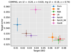
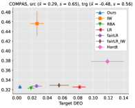
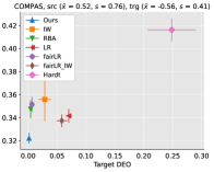
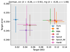
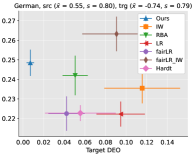
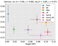
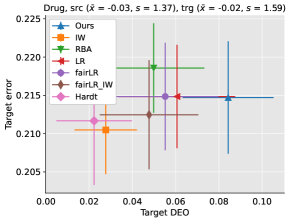
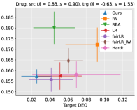
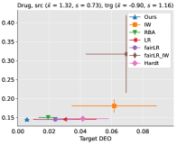
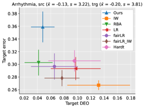
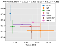
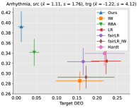
Figure 2: Average prediction error versus average difference of equalized opportunity (DEO) on target samples. The bar is the 95% confidence interval on ten random biased samplings on the first principal component of the covariates ($P_{\text{src}}(x,a)\neq P_{\text{trg}}(x,a)$).

Baseline methods

We evaluate the performance of our model in terms of the trade-off between prediction error and fairness violation on target under various intensities of covariate shift. We focus on equalized opportunity as our fairness definition. We compare against the following baselines:

• Logistic Regression (LR) is the standard logistic regression predictor trained on source data, ignoring both covariate shift and desired fairness properties.

• Robust Bias-Aware Log Loss Classifier (RBA) (Liu and Ziebart 2014) in (6) which accounts for the covariate shift but ignores fairness.

• Sample Re-weighted Logistic Regression (LR_IW) (Shimodaira 2000) minimizes the re-weighted log loss on the source data, according to the importance weighting scheme (5): it only accounts for the covariate shift.

• Post Processing (Hardt) transforms the logistic regression target output to adjust for true positive rate parity (Hardt, Price, and Srebro 2016); ignores covariate shift.

• Fair Logistic Regression (fairLR) also optimizes worst-case log loss subject to fairness as linear constraints with observed labels on source data (Rezaei et al. 2020). It accounts for fairness, but ignores the covariate shift.

• Sample Re-weighted Fair Logistic Regression (fairLR_IW) the fairLR method augmented with importance weighting scheme (5) in training. This baseline account for both fairness and covariate shift.

Setup

We repeat our sampling procedure for each dataset ten times and report the average prediction error and the average difference of equalized opportunity (DEO): $|\mathbb{P}(\widehat{Y}=1|A=1,Y=1)-\mathbb{P}(\widehat{Y}=1|A=0,Y=1)|$ of our predictor on the target dataset.

Unfortunately since the target distribution is assumed to be unavailable for this problem, properly obtaining optimal regularization via cross validation is not possible. We select the L2 regularization parameter by choosing the best $C$ from $\{10^{-5},10^{-4},10^{-3},10^{-2},10^{-1},1,10\}$ under the IID assumption. We use first-order features for our implementation, i.e., $\phi(\mathbf{x},y)=[x_{1}y,x_{2}y,\dots x_{m}y]^{\top}$, where $m$ is the size of features. Under the mild assumption that the estimated fairness violation by $\mathbb{Q}$ remains monotone given sufficiently expressive feature constraints on source and group marginal constraints of target, we find the exact zero point of the approximated violation efficiently by binary search for $\mu\in[-1.5,1.5]$ in our experiments.

We create samplings based on three parameter settings for $(\alpha,\beta)\in\{(0,1),(1,2),(1.5,3)\}$ which is the left, middle and right column in Figure 2 respectively. The left column is the closest sampling to IID, as the prior sampling densities are identical. However, due to the large sampling size without replacement, the actual samples can vary quite significantly from the Gaussian prior density, as can be seen by the actual sample mean and standard deviation reported on top of each plot. The accuracy of estimated density ratios has a crucial impact on the performance of our model and covariate shift correction in general. We employ 2D Gaussian kernel density estimation (KDE) with bandwidth $\sigma=0.3$ on the first two principal components of the covariates in each sample to re-estimate the actual densities $d_{i}$ for the $i^{\text{th}}$ data point in the source and target distributions. In order to control the magnitude of the ratios and avoid extremely large values, we normalize the densities on source and target by $p_{i}=(d_{i}+\epsilon)/(\sum_{i}^{n}(d_{i}+\epsilon))$, where $n$ is the size of each set. We set $\epsilon=0.001$ for the smaller Arrhythmia dataset and $\epsilon=0.01$ for the rest of the datasets.

Results

Figure 2 shows our experimental results on three samplings from close to IID (left) to mild (middle) and strong covariate shift (right). Figure 1 provides an example of these samplings on German. On the COMPAS dataset, our method consistently achieves the lowest DEO while also keeping the lowest prediction error as the shift increases, while the Hardt method’s DEO worsen with the increasing shift. The optimal $\mu$ lies consistently close to zero on larger shifts on this dataset, which explains why RBA and FairLR are also very close to our method, indicating that the created shift was positively correlated to fairness. On the German dataset, our method provides the lowest and closest to zero average DEO on all shifted samplings, with competitive prediction error compared to other baselines. As the shift intensifies DEO worsens for other baselines (except RBA), which shows the negative effect of covariate shift on fairness for this dataset. On the Drug dataset, our method’s DEO starts high. However, as the shift intensifies, our method outperforms other baselines on DEO while having equally low error as other competitive baselines. We have observed high sensitivity of results for our method and RBA to the accuracy of density ratios on instances of this dataset with lower shift intensity. 2D KDE provides significant improvement over 1D in this regard. We believe more accurate density estimation in higher dimensions should improve the consistency of these results. The samples on Arrhythmia are much smaller and have larger standard deviation compared to the other datasets. Our method achieves the lowest fairness violation at the cost of incurring slightly higher error compared to other baselines on this dataset.

In summary, our method achieves lowest DEO on 10 out of 12 samplings in our experiments. In four of those samplings, our method is equal with or outperforms the best baselines on prediction error as well, while being competitive for prediction error on the rest. These experiments show the overall effectiveness of our fair prediction method under general shift in the covariates.

Conclusions

In this paper, we developed a novel adversarial approach for seeking fair decision making under covariate shift. In contrast with importance weighting methods, our approach is designed to operate appropriately even when portions of the shift between source and target distributions are extreme. The key technical challenge we address is the lack of labeled target data points, making target fairness assessment challenging. We instead propose to measure approximated fairness against an worst-case adversary that is constrained by source data properties and group marginals from target. We incorporate fairness as a weighted penalty and tune the weighted penalty to provide fairness against the adversary. More extensive evaluation on naturally-biased datasets and generalization of this approach to decision problems beyond binary classification are both important future directions.

Broader Impact

Fairness considerations are increasingly important for machine learning systems applied to key social applications. However, the standard assumptions of statistical machine learning, such as iid training and testing data, are often violated in practice. This work offers an approach for robustly seeking fair decisions in such settings and could be of general benefit to individuals impacted by alternative systems that are either oblivious or brittle to these broken assumptions. However, this work also makes a covariate shift assumption instead of accounting for more specific causal relations that may generate the shift. Practitioners should be aware of the specific assumptions made by this paper.

References

- Adel et al. (2019) Adel, T.; Valera, I.; Ghahramani, Z.; and Weller, A. 2019. One-network Adversarial Fairness. In AAAI.
- Agarwal et al. (2018) Agarwal, A.; Beygelzimer, A.; Dudík, M.; Langford, J.; and Wallach, H. M. 2018. A Reductions Approach to Fair Classification. In ICML.
- Awasthi, Kleindessner, and Morgenstern (2020) Awasthi, P.; Kleindessner, M.; and Morgenstern, J. 2020. Equalized odds postprocessing under imperfect group information. In International Conference on Artificial Intelligence and Statistics, 1770–1780. PMLR.
- Azizzadenesheli et al. (2019) Azizzadenesheli, K.; Liu, A.; Yang, F.; and Anandkumar, A. 2019. Regularized learning for domain adaptation under label shifts. arXiv preprint arXiv:1903.09734 .
- Barocas, Hardt, and Narayanan (2017) Barocas, S.; Hardt, M.; and Narayanan, A. 2017. Fairness in machine learning. NIPS Tutorial .
- Bechavod and Ligett (2017) Bechavod, Y.; and Ligett, K. 2017. Penalizing unfairness in binary classification. arXiv preprint arXiv:1707.00044 .
- Ben-David et al. (2007) Ben-David, S.; Blitzer, J.; Crammer, K.; and Pereira, F. 2007. Analysis of representations for domain adaptation. In Advances in neural information processing systems, 137–144.
- Blitzer et al. (2008) Blitzer, J.; Crammer, K.; Kulesza, A.; Pereira, F.; and Wortman, J. 2008. Learning bounds for domain adaptation. In Advances in neural information processing systems, 129–136.
- Boyd and Vandenberghe (2004) Boyd, S.; and Vandenberghe, L. 2004. Convex optimization. Cambridge university press.
- Calders, Kamiran, and Pechenizkiy (2009) Calders, T.; Kamiran, F.; and Pechenizkiy, M. 2009. Building classifiers with independency constraints. In ICDMW ’09.
- Calmon et al. (2017) Calmon, F.; Wei, D.; Vinzamuri, B.; Natesan Ramamurthy, K.; and Varshney, K. R. 2017. Optimized Pre-Processing for Discrimination Prevention. In NeurIPS.
- Carter and Catlett (1987) Carter, C.; and Catlett, J. 1987. Assessing credit card applications using machine learning. IEEE Expert .
- Celis et al. (2019) Celis, L. E.; Huang, L.; Keswani, V.; and Vishnoi, N. K. 2019. Classification with fairness constraints: A meta-algorithm with provable guarantees. In ACM FAT*.
- Celis and Keswani (2019) Celis, L. E.; and Keswani, V. 2019. Improved Adversarial Learning for Fair Classification. arXiv preprint .
- Chang (2006) Chang, L. 2006. Applying data mining to predict college admissions yield: A case study. NDIR .
- Chierichetti et al. (2017) Chierichetti, F.; Kumar, R.; Lattanzi, S.; and Vassilvitskii, S. 2017. Fair clustering through fairlets. In Advances in Neural Information Processing Systems, 5029–5037.
- Cortes, Mansour, and Mohri (2010) Cortes, C.; Mansour, Y.; and Mohri, M. 2010. Learning bounds for importance weighting. In Advances in neural information processing systems, 442–450.
- Cotter et al. (2018) Cotter, A.; Jiang, H.; Wang, S.; Narayan, T.; Gupta, M.; You, S.; and Sridharan, K. 2018. Optimization with non-differentiable constraints with applications to fairness, recall, churn, and other goals. arXiv preprint .
- Daume III and Marcu (2006) Daume III, H.; and Marcu, D. 2006. Domain adaptation for statistical classifiers. Journal of artificial Intelligence research 26: 101–126.
- Del Barrio et al. (2018) Del Barrio, E.; Gamboa, F.; Gordaliza, P.; and Loubes, J.-M. 2018. Obtaining fairness using optimal transport theory. arXiv preprint .
- Dheeru and Karra Taniskidou (2017) Dheeru, D.; and Karra Taniskidou, E. 2017. UCI Machine Learning Repository. URL http://archive.ics.uci.edu/ml.
- Donini et al. (2018) Donini, M.; Oneto, L.; Ben-David, S.; Shawe-Taylor, J. S.; and Pontil, M. 2018. Empirical risk minimization under fairness constraints. In NeurIPS.
- Dwork et al. (2012) Dwork, C.; Hardt, M.; Pitassi, T.; Reingold, O.; and Zemel, R. 2012. Fairness through awareness. In ITCS.
- Dwork et al. (2017) Dwork, C.; Immorlica, N.; Kalai, A. T.; and Leiserson, M. 2017. Decoupled classifiers for fair and efficient machine learning. arXiv preprint arXiv:1707.06613 .
- Fehrman et al. (2017) Fehrman, E.; Muhammad, A. K.; Mirkes, E. M.; Egan, V.; and Gorban, A. N. 2017. The five factor model of personality and evaluation of drug consumption risk. In Data science, 231–242. Springer.
- Feldman et al. (2015) Feldman, M.; Friedler, S. A.; Moeller, J.; Scheidegger, C.; and Venkatasubramanian, S. 2015. Certifying and removing disparate impact. In ACM SIGKDD.
- Goel, Yaghini, and Faltings (2018) Goel, N.; Yaghini, M.; and Faltings, B. 2018. Non-discriminatory machine learning through convex fairness criteria. In AAAI.
- Gretton et al. (2009) Gretton, A.; Smola, A.; Huang, J.; Schmittfull, M.; Borgwardt, K.; and Schölkopf, B. 2009. Covariate shift by kernel mean matching. Dataset shift in machine learning 3(4): 5.
- Grünwald and Dawid (2004) Grünwald, P. D.; and Dawid, A. P. 2004. Game Theory, Maximum Entropy, Minimum Discrepancy, and Robust Bayesian Decision Theory. Annals of Statistics 32.
- Guidotti et al. (2018) Guidotti, R.; Monreale, A.; Ruggieri, S.; Turini, F.; Giannotti, F.; and Pedreschi, D. 2018. A survey of methods for explaining black box models. ACM computing surveys (CSUR) 51(5): 1–42.
- Hardt, Price, and Srebro (2016) Hardt, M.; Price, E.; and Srebro, N. 2016. Equality of opportunity in supervised learning. In NeurIPS.
- Jabbari et al. (2016) Jabbari, S.; Joseph, M.; Kearns, M.; Morgenstern, J.; and Roth, A. 2016. Fair learning in markovian environments. arXiv preprint arXiv:1611.03071 .
- Kabakchieva (2013) Kabakchieva, D. 2013. Predicting student performance by using data mining methods for classification. Cybernetics and Information Technologies 13(1).
- Kamiran and Calders (2012) Kamiran, F.; and Calders, T. 2012. Data preprocessing techniques for classification without discrimination. Knowledge and Information Systems 33(1).
- Kamishima, Akaho, and Sakuma (2011) Kamishima, T.; Akaho, S.; and Sakuma, J. 2011. Fairness-aware learning through regularization approach. In ICDMW.
- Lamy et al. (2019) Lamy, A.; Zhong, Z.; Menon, A. K.; and Verma, N. 2019. Noise-tolerant fair classification. In Advances in Neural Information Processing Systems, 294–306.
- Larson et al. (2016) Larson, J.; Mattu, S.; Kirchner, L.; and Angwin, J. 2016. How we analyzed the COMPAS recidivism algorithm. ProPublica 9.
- Lipton, Wang, and Smola (2018) Lipton, Z. C.; Wang, Y.-X.; and Smola, A. 2018. Detecting and correcting for label shift with black box predictors. arXiv preprint arXiv:1802.03916 .
- Liu and Ziebart (2014) Liu, A.; and Ziebart, B. 2014. Robust Classification Under Sample Selection Bias. In NeurIPS.
- Lohr (2013) Lohr, S. 2013. Big data, trying to build better workers. The New York Times 21.
- Madras et al. (2018) Madras, D.; Creager, E.; Pitassi, T.; and Zemel, R. 2018. Learning adversarially fair and transferable representations. arXiv preprint .
- Mehrabi et al. (2019) Mehrabi, N.; Morstatter, F.; Saxena, N.; Lerman, K.; and Galstyan, A. 2019. A survey on bias and fairness in machine learning. arXiv preprint arXiv:1908.09635 .
- Menon and Williamson (2018) Menon, A. K.; and Williamson, R. C. 2018. The cost of fairness in binary classification. In ACM FAT*.
- Moses and Chan (2014) Moses, L. B.; and Chan, J. 2014. Using big data for legal and law enforcement decisions: Testing the new tools. UNSWLJ .
- Obermeyer and Emanuel (2016) Obermeyer, Z.; and Emanuel, E. J. 2016. Predicting the future—big data, machine learning, and clinical medicine. The New England Journal of Medicine 375(13).
- O’Neil (2016) O’Neil, C. 2016. Weapons of math destruction: How big data increases inequality and threatens democracy. Broadway Books.
- Pedreshi, Ruggieri, and Turini (2008) Pedreshi, D.; Ruggieri, S.; and Turini, F. 2008. Discrimination-aware data mining. In Proceedings of the 14th ACM SIGKDD international conference on Knowledge discovery and data mining, 560–568.
- Pleiss et al. (2017) Pleiss, G.; Raghavan, M.; Wu, F.; Kleinberg, J.; and Weinberger, K. Q. 2017. On Fairness and Calibration. In NeurIPS.
- Quadrianto and Sharmanska (2017) Quadrianto, N.; and Sharmanska, V. 2017. Recycling privileged learning and distribution matching for fairness. In NeurIPS.
- Rezaei et al. (2020) Rezaei, A.; Fathony, R.; Memarrast, O.; and Ziebart, B. 2020. Fairness for Robust Log Loss Classification. In AAAI.
- Schölkopf et al. (2012) Schölkopf, B.; Janzing, D.; Peters, J.; Sgouritsa, E.; Zhang, K.; and Mooij, J. 2012. On causal and anticausal learning. arXiv preprint arXiv:1206.6471 .
- Scott, Blanchard, and Handy (2013) Scott, C.; Blanchard, G.; and Handy, G. 2013. Classification with asymmetric label noise: Consistency and maximal denoising. In Conference On Learning Theory, 489–511.
- Shaw and Gentry (1988) Shaw, M. J.; and Gentry, J. A. 1988. Using an expert system with inductive learning to evaluate business loans. Financial Management .
- Shimodaira (2000) Shimodaira, H. 2000. Improving predictive inference under covariate shift by weighting the log-likelihood function. Journal of statistical planning and inference 90(2): 227–244.
- Shipp et al. (2002) Shipp, M. A.; Ross, K. N.; Tamayo, P.; Weng, A. P.; Kutok, J. L.; Aguiar, R. C.; Gaasenbeek, M.; Angelo, M.; Reich, M.; Pinkus, G. S.; et al. 2002. Diffuse large B-cell lymphoma outcome prediction by gene-expression profiling and supervised machine learning. Nature medicine 8(1).
- Singh et al. (2019) Singh, H.; Singh, R.; Mhasawade, V.; and Chunara, R. 2019. Fair Predictors under Distribution Shift. arXiv preprint arXiv:1911.00677 .
- Sugiyama, Krauledat, and Müller (2007) Sugiyama, M.; Krauledat, M.; and Müller, K.-R. 2007. Covariate shift adaptation by importance weighted cross validation. Journal of Machine Learning Research 8(May): 985–1005.
- Topsøe (1979) Topsøe, F. 1979. Information-theoretical optimization techniques. Kybernetika 15(1): 8–27.
- Verma and Rubin (2018) Verma, S.; and Rubin, J. 2018. Fairness definitions explained. In 2018 IEEE/ACM International Workshop on Software Fairness (FairWare), 1–7. IEEE.
- Woodworth et al. (2017) Woodworth, B.; Gunasekar, S.; Ohannessian, M. I.; and Srebro, N. 2017. Learning Non-Discriminatory Predictors. In COLT.
- Xu et al. (2018) Xu, D.; Yuan, S.; Zhang, L.; and Wu, X. 2018. FairGAN: Fairness-aware generative adversarial networks. In IEEE Big Data.
- Yang et al. (2020) Yang, K.; Qinami, K.; Fei-Fei, L.; Deng, J.; and Russakovsky, O. 2020. Towards fairer datasets: Filtering and balancing the distribution of the people subtree in the imagenet hierarchy. In Proceedings of the 2020 Conference on Fairness, Accountability, and Transparency, 547–558.
- Zafar et al. (2017a) Zafar, M. B.; Valera, I.; Gomez Rodriguez, M.; and Gummadi, K. P. 2017a. Fairness beyond disparate treatment & disparate impact: Learning classification without disparate mistreatment. In WWW.
- Zafar et al. (2017b) Zafar, M. B.; Valera, I.; Rodriguez, M.; Gummadi, K.; and Weller, A. 2017b. From parity to preference-based notions of fairness in classification. In NeurIPS.
- Zafar et al. (2017c) Zafar, M. B.; Valera, I.; Rogriguez, M. G.; and Gummadi, K. P. 2017c. Fairness Constraints: Mechanisms for Fair Classification. In AISTATS.
- Zemel et al. (2013) Zemel, R.; Wu, Y.; Swersky, K.; Pitassi, T.; and Dwork, C. 2013. Learning Fair Representations. In ICML.
- Zhang, Lemoine, and Mitchell (2018) Zhang, B. H.; Lemoine, B.; and Mitchell, M. 2018. Mitigating unwanted biases with adversarial learning. In AIES.