Deep Imitation Learning for Bimanual
Robotic Manipulation

Abstract

We present a deep imitation learning framework for robotic bimanual manipulation in a continuous state-action space. A core challenge is to generalize the manipulation skills to objects in different locations. We hypothesize that modeling the relational information in the environment can significantly improve generalization. To achieve this, we propose to (i) decompose the multi-modal dynamics into elemental movement primitives, (ii) parameterize each primitive using a recurrent graph neural network to capture interactions, and (iii) integrate a high-level planner that composes primitives sequentially and a low-level controller to combine primitive dynamics and inverse kinematics control. Our model is a deep, hierarchical, modular architecture. Compared to baselines, our model generalizes better and achieves higher success rates on several simulated bimanual robotic manipulation tasks. We open source the code for simulation, data, and models at: https://github.com/Rose-STL-Lab/HDR-IL.

1 Introduction

Manipulation is a fundamental capability robots need for many real-world applications. Although there has been significant progress in single-arm manipulation tasks such as grasping, pick-and-place, and pushing [1, 2, 3, 4], bimanual manipulation has received less attention. Many tasks however require using both arms/hands; consider opening a bottle, steadying a nail while hammering, or moving a table. While having two arms to accomplish these tasks is clearly useful, bimanual manipulation tasks are also significantly more challenging, due to higher-dimensional continuous state-action spaces, more object interactions, and longer-horizon solutions.

Most existing work in bimanual manipulation addresses the problem in a classical control setting, where the environment and its dynamics are known [5]. However, these models are difficult to construct explicitly and are inaccurate, because of complicated interactions in the task including friction, adhesion, and deformation between the two arms/hands and the object being manipulated. A promising approach that avoids manually specifying models is imitation learning, where a teacher provides demonstrations of desired behavior to the robot (sequences of sensed input states and target control actions in those states), and the robot learns a policy to mimic the teacher [6, 7, 8]. In particular, recent deep imitation learning methods have been successful at learning single-arm manipulation from demonstrations, even with only images as observations (e.g., [9, 10]).

In this work, we explore extending deep imitation learning methods to bimanual manipulation. In light of the challenges identified above, our goal is to design an imitation learning model to capture relational information (i.e., the trajectory involves relations to other objects in the environment) in environments with complex dynamics (i.e., the task requires multiple object interactions to accomplish a goal). The model needs to be general enough to complete tasks under different variations, such as changes in the initial configuration of the robot and objects.

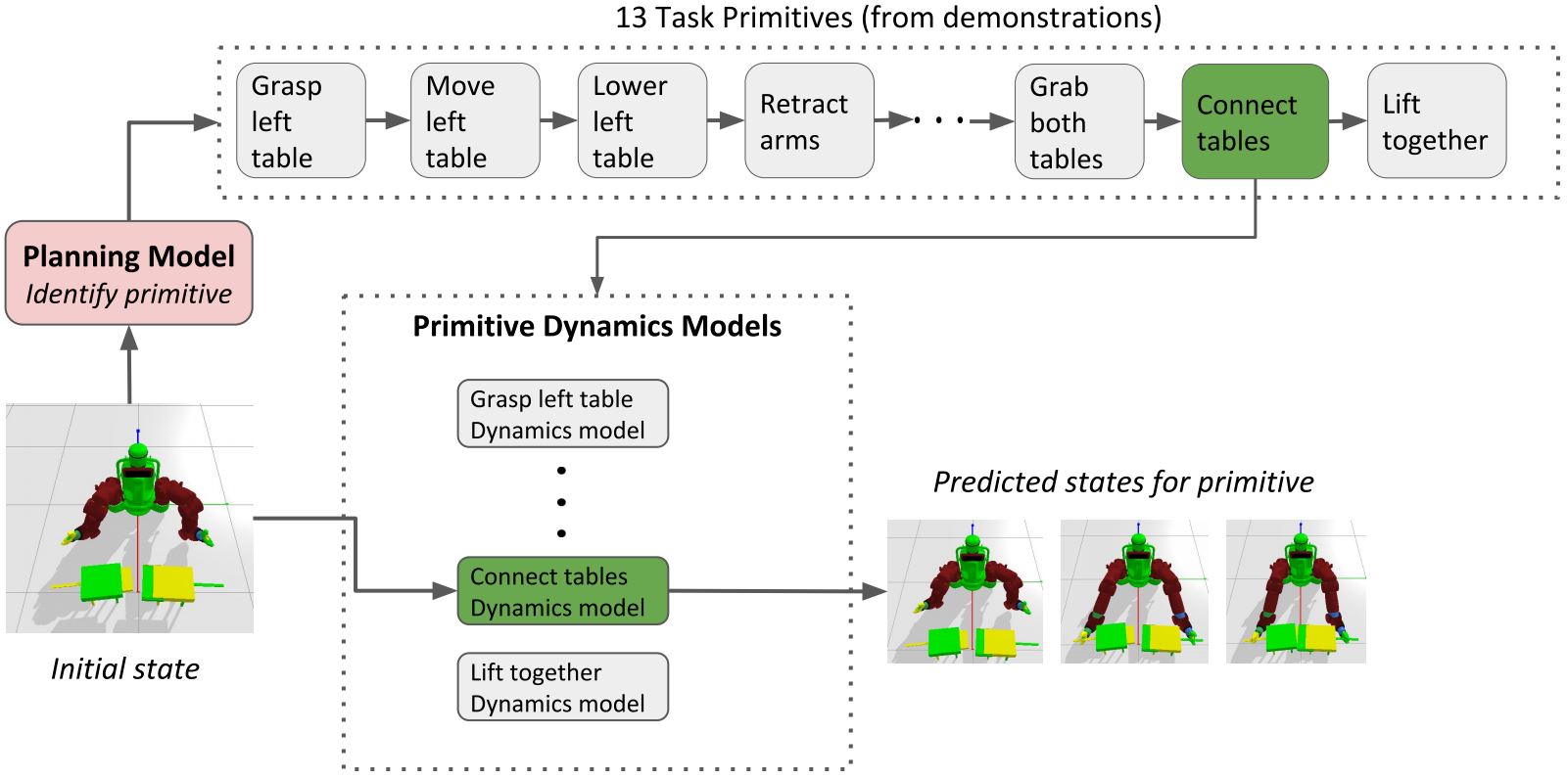
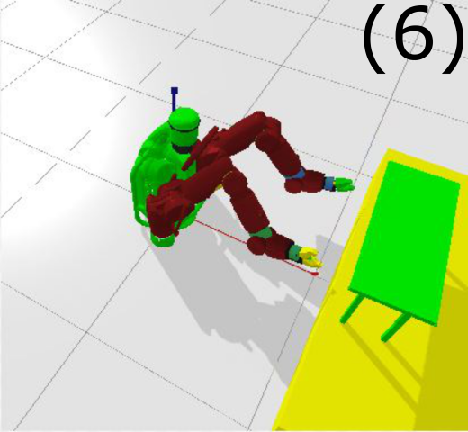
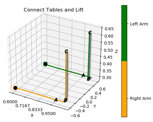
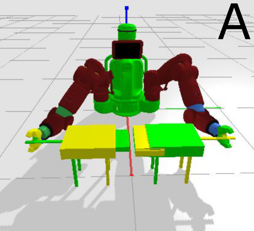
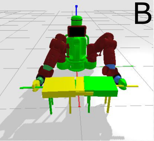
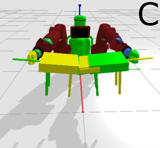
The insight of our paper is to accomplish this goal through a two-level framework, illustrated in Figure 1 for a bimanual “peg-in-hole” table assembly and lifting task. The task involves grasping two halves of a table, slotting one half into the other, and then lifting both parts together as whole. Instead of trying to learn a policy for the entire trajectory, we split demonstrations into task primitives (subsequences of states), as shown in the top row. We learn two models: a high-level planning model that predicts a sequence of primitives, and a set of low-level primitive dynamics models that predict a sequence of robot states to complete each identified task primitive. All models are parameterized by recurrent graph neural networks that explicitly capture robot-robot and robot-object interactions. In summary, our contributions include:

• We propose a deep imitation learning framework, Hierarchical Deep Relational Imitation Learning (HDR-IL), for robotic bimanual manipulation. Our model explicitly captures the relational information in the environment with multiple objects.

• We take a hierarchical approach by separately learning a high-level planning model and a set of low-level primitive dynamics models. We incorporate relational features and use recurrent graph neural networks to parameterize all models.

• We evaluate on two variations of a table-lifting task where bimanual manipulation is essential. We show that both hierarchical and relational modeling provide significant improvement for task completion on held-out instances. For the task shown in Figure 1, our model achieves $29\%$ success rate, whereas a baseline approach without these contributions only succeeds in $1\%$ of the test cases.

Figure 1: An example of the HDR-ILmodel performing a “peg-in-hole” construction of a table. The trajectory of primitives to complete this task is shown in the top row. The sequence of high-level primitives is learned from demonstrations. State trajectories are predicted based on the primitive identified. The final predicted state for the primitive becomes the initial state for the next primitive.

2 Related Work

The idea of abstracting temporally extended actions has been studied in hierarchical reinforcement learning (HRL) for decades, with the goal of reducing the action search space and sample complexity [11, 12]. A special and useful case is the concept of parameterized skills, or primitives, where skills are pre-defined and the sequence of skills are learned [13]. Such a hierarchical modeling approach has been widely used in robotics and reinforcement learning [14, 15, 16, 17, 18]. This results in a more structured discrete-continuous action space. The learning for this action space can be naturally decomposed into multiple phases with different primitives applied [19].

Prior work on learning sequences of skills using demonstrations [20, 21, 19, 22, 23] either rely on pre-defined primitive functions or statistical models such as hidden Markov models. Pre-defined primitive functions can be restrictive in representing complex dynamics. Recently, [24, 25] applied pretrained deep neural networks to identify primitives from input states. Hierarchical imitation learning [26, 27, 28] learns the primitives from demonstrations, but does not use relational models.

Our main contribution is learning more accurate dynamics models to support imitation learning of bimanual robotic manipulation tasks. [29] learns a latent representation space to decouple high-level effects and low-level motions, which follows the idea of disentangling the learning into two levels. Recently, graph neural networks (GNNs) [30] have been used to model complex physical dynamics in several applications. Graph models have been used to model physical interaction between objects such as particles [31], [32] and other rigid objects [33], [34]. In the robotics domain, one common approach is to model robots as graphs comprised of nodes corresponding to joints and edges corresponding to links on the robot body, e.g., [35].

3 Background

We describe imitation learning using the Markov Decision Process (MDP) framework. An MDP is defined as a tuple $\langle\mathcal{S},\mathcal{A},T,R,\gamma\rangle$, where $\mathcal{S}$ is the state space, $\mathcal{A}$ is the action space, $T:\mathcal{S\times A}\rightarrow\Delta(S)$ is the transition function, $R:\mathcal{S}\times\mathcal{A}\rightarrow\mathbb{R}$ is the reward function, and $\gamma$ is the discount factor. In imitation learning, we are given a collection of demonstrations $\{\tau^{(i)}=(s_{1},a_{1},\cdots)\}_{i=1}^{D}$ from an expert policy $\pi_{E}$, and the objective is to learn a policy $\pi_{\theta}$ from $\{\tau^{(i)}\}_{i=1}^{D}$ that mimics the expert policy. Imitation learning requires a larger number of demonstrations for long horizon problems, which can be alleviated with hierarchical imitation learning [27].

In hierarchical imitation learning, there is typically a two-level hierarchy: a high-level planning policy and a low-level control policy. The high-level planning policy $\pi_{h}$ generates a primitive sequence $(p^{1},p^{2},\cdots)$. In robotic manipulation, a primitive $p^{k}\in\mathcal{P}$ corresponds to a parameterized policy that maps states to actions $\pi_{p^{k}}:\mathcal{S}\rightarrow{\mathcal{A}}$, that are typically used to achieve subgoals such as grasping and lifting. Each primitive $p^{k}$ results in a low-level state trajectory $(s^{k}_{1},s^{k}_{2},\cdots)$. Given a primitive $p^{k}$ and the initial state $s_{t}$ , we aim to learn a policy to produce a sequence of states which can be used by an inverse kinematics (IK) solver to obtain the robot control actions $(a^{k}_{1},a^{k}_{2},\cdots)$.

4 Methodology

Figure 2: HDR-IL Pipeline: The planning model learns sequences of primitives from demonstrations of the task. The primitive dynamics model takes an initial state and the learned sequence of primitives to predict future states (robot and object poses) for the task. Finally, we use inverse kinematics to compute low-level robot controls needed to reach the predicted states and execute the commands using the PyBullet physics simulator. The high-level planning allows the identification of primitives, which are used to select the appropriate primitive dynamics model Multi. Within each primitive’s dynamics model, the GNN layers Int capture interactions between objects. The residual connection Res of the object state helps direct the projection towards the target. Additional implementation details and hyperparameter settings are found in the supplementary material.

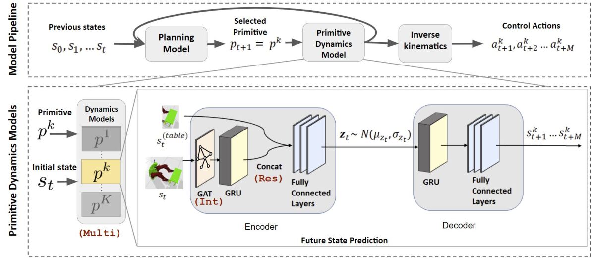
We propose a hierarchical framework for planning and control in robotic bimanual manipulation, outlined in Figure 2. Our framework combines a high-level planning model and a low-level primitive dynamics model to forecast a sequence of $N$ states. We divide the sequence of $N$ states into $K$ primitives $p_{1},\cdots,p_{K}$, with each primitive consisting of a trajectory with a fixed number of states $M=N/K$. A high-level planning model selects the primitive based on previous states ($s_{0},...s_{t-1})\mapsto p_{t}$. A low-level primitive dynamics model uses the selected primitive $p_{t}=p^{k}$, and predicts the next $M$ steps $s_{t-1}\mapsto(s^{k}_{t}...s^{k}_{t+M})$. An inverse kinematics solver then translates a sequence of states into robot control actions $(a^{k}_{1},a^{k}_{2},\cdots)$. We first detail the low-level control model and our contributions to this model. The high-level planning model shares many architectural features with the low-level control model.

4.1 Low-level Control Model

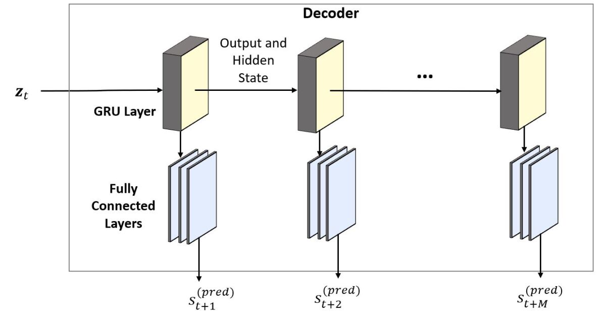
Sequence to sequence models [36] with recurrent neural networks (RNN) have been used effectively in prior deep imitation learning methods, e.g. [37]. In our model, we introduce a stochastic component through a variational auto-encoder [38] to generate a latent state distribution $Z_{t}\sim\mathcal{N}(\mu_{z_{t}},\sigma_{z_{t}})$. The decoder samples a latent state $z_{t}$ from the distribution and generates a sequence of outputs. We build on this design and innovate in several aspects to execute high-precision bimanual manipulation tasks.

Relational Features (Int)

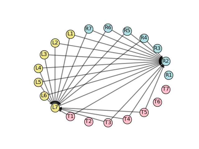
The vanilla RNN encoder-decoder model assumes different input features are independent whereas robot arms and objects have strong dependency. To capture these relational dependencies, we introduce a graph attention (GAT) layer [39] in the encoder, leading to graph RNN. We construct a fully connected graph where each node corresponds to each feature dimension in the state. The attention mechanism of the GAT model learns edge weights through training. Specifically, given two objects features $h_{u}$ and $h_{v}$, we compute the edge attention coefficients $e_{uv}$ according to the GAT attention update $e_{uv}=a(\mathbf{W}h_{u},\mathbf{W}h_{v})$. Here $\mathbf{W}$ are shared trainable weights. These coefficients are used to obtain the attention: $\alpha_{uv}=\mathrm{softmax}(e_{uv})$. The GAT feature update is given by $h_{u}=\sigma\left(\sum_{v\in\mathcal{N}_{u}}\alpha_{uv}\mathbf{W}h_{v}\right)$ where ${\mathcal{N}}_{u}$ is the neighbour nodes of $u$. This model allows us to learn parameters that capture the relational information between the objects. The GAT layer that processes the relational features is shown with Int in Figure 2.

Residual Connection (Res)

Another key component of our dynamics model is a residual skip connection that connects features of the target object, such as the table to be moved, to the last hidden layer of the encoder GRU [40]. This idea was inspired by previous robotics work where motor primitives are defined by a dynamics function and a goal state [21]. Skip connections were also used in [41] to help learn complex features in an encoder. The inclusion of the skip connection here helps emphasize the goal, in this case the target object features. This is shown as Res in Figure 2.

Modular Movement Primitives (Multi)

Primitives represent elementary movement patterns such as grasping, lifting and turning. A shared model for all primitive dynamics is limited in its representation power and generalization to more complex tasks. Instead, we take a modular approach at modeling the primitive dynamics. In particular, we design a separate neural network module for each primitive. Each neural network hence captures a particular type of primitive dynamics. We use the same Graph RNN architecture with residual connections for each primitive module. For a task comprised of $K$ ordered primitives with $M$ steps each, each module approximate the primitive policy $\pi_{p^{k}}$, which produces a state trajectory $(s_{1}^{k},s_{2}^{k},\cdots)$. The last state of each primitive is used as the initial state for the next primitive, which is predicted by the high-level planning model.

Inverse Kinematics Controller

In robotics, inverse kinematics (IK) calculates the variable joint parameters needed to place the end of a robot manipulator in a given position and orientation relative to the start. An IK function is used to translate the sequence of states to the control commands for the robot. At each time step, the predicted state for the robot grippers is taken as the input to the IK solver. IK is an iterative algorithm that calculates the robot joint angles needed to reach the desired gripper position. These angles determine the commands on each joint to execute robot movement.

4.2 High-level Planning Model

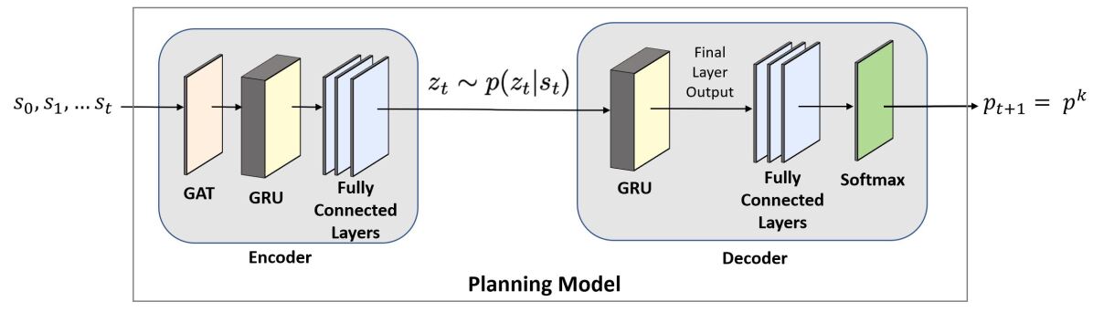
The goal of the high-level planning model is to learn a policy $\pi_{h}$ which maps a sequence of observed states to a sequence of predefined primitives $\pi_{h}:{\mathcal{S}}\rightarrow{\mathcal{P}}$. Each identified primitive $p^{k}$ selects the corresponding primitive dynamics policy $\pi_{p^{k}}$, which is then used for low-level control. Our planning model takes all previous states and infers the next primitive $s_{0},s_{1},..s_{t-1}\mapsto p_{t}$.

Similar to the low-level control model, capturing object interaction in the environment is crucial to accurate predictions of the primitive sequence. Hence, we use the same graph RNN model described in Section 4.1 and introduce relational features Int in the input. We omit the residual connections as we did not find them necessary for the primitive identification. An architecture visualization is provided in the Appendix Section A.4.

4.3 Supervised Training

The planning model and the control model are trained separately in a supervised learning fashion. We train the high-level planning model on manually labeled demonstrations, in order to map a sequence of states $s_{1},\cdots,s_{t-1}$ into a primitive label $p_{t}=k\in[1,\dots,K]$. The labels are learned with supervision of the correct primitive for the task using the cross entropy loss. The primitive dynamics model is trained end-to-end with mean-square error loss on each predicted state $\hat{s}_{t}$ across all time steps. In the multi-model framework, each primitive is trained with its own parameters for the dynamics model.

5 Experiments

We evaluate our approach in simulation using two table lifting tasks which require high precision bimanual manipulation to succeed. We demonstrate the generalization of our model by testing the model with different table starting locations.

5.1 Experimental Setup

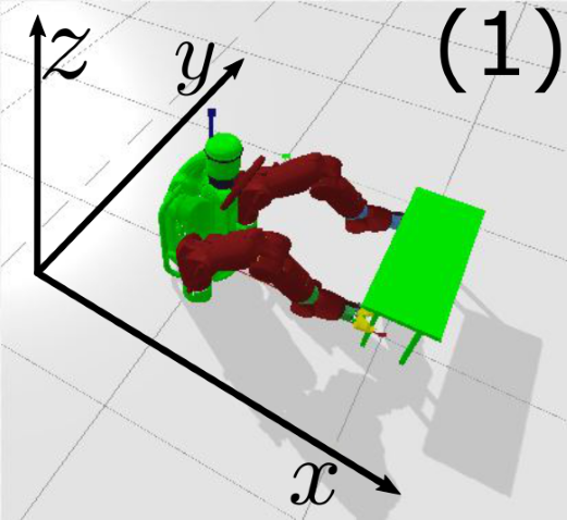
All simulations for this study were conducted using the PyBullet [42] physics simulator with a Baxter robot. Baxter operates using two arms, each with 7 degrees of freedom. We designed our environment using URDF objects with various weightless links to track location. Our data consists of the $xyz$ coordinates and 4 quaternions for the robot grippers and each object in the environment.

Demonstrations were manually labeled as separate primitives in the simulator and sequenced together to generate the simulation data. Each primitive function was parameterized so they can adapt to different starting and ending coordinates. The primitives were selected such that they each had a distinct trajectory dynamic (ie. lifting upwards vs moving sideways). Each primitive generated a sequence of between 10-12 states for the robot grippers. The number of states were selected through experimentation with the simulation. A minimum number of states were needed for each primitive to produce a smooth non-linear trajectory, while too many states increased the complexity for predictions. We then used the inverse kinematics function to translate the states into command actions for the robot simulator.

Models

We compare and evaluate several model designs in our experiments. Details about the design elements are in Section 4. The models we consider are:

• GRU Encoder-Decoder Model (GRU-GRU): Single model with an GRU encoder, GRU decoder.

• Interaction Network Model (Int): This is the GRU-GRU model with a fully connected graph network and a graph attention layer, equivalent to feature Int in Figure 2.

• Residual Link Model (Res): The GRU-GRU model with skip connection for the table features, equivalent to feature Res in Figure 2.

• Residual Interaction Model (ResInt): The GRU-GRU model with combined graph structure and skip connection of table object features, equivalent to adding features Res  and Int in Figure 2.

• HDR-IL Model: Our multi-model framework which uses multiple ResInt models, one model for each primitive. The appropriate model is chosen by the Multimodule shown in Figure 2.

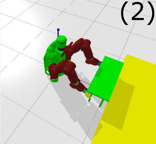
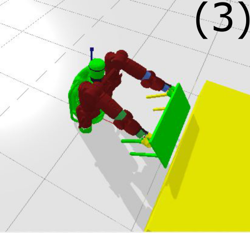
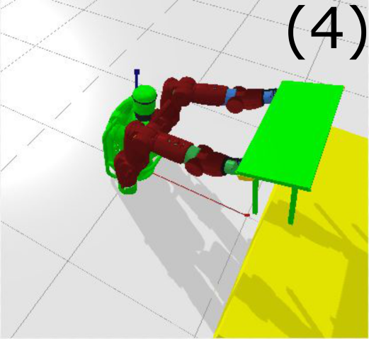
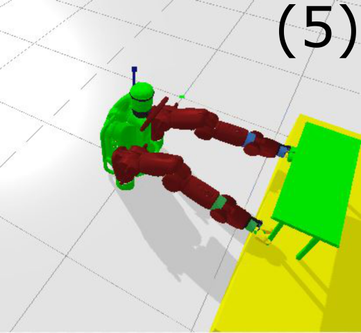
5.2 Table Lifting Task

Task Design

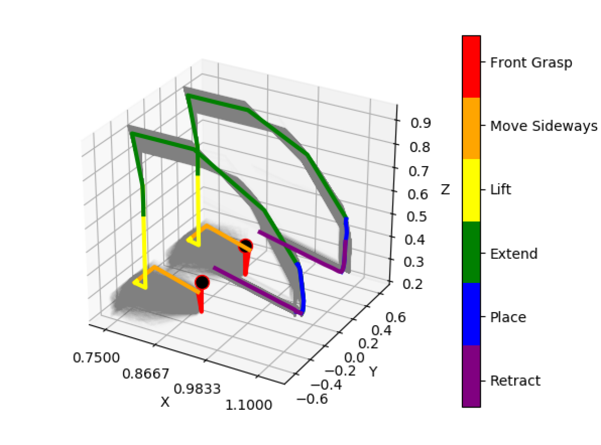
In this task, our robot is tasked to lift a table, with dimensions 35cm by 85cm, onto a platform. We measured success as the table landing upright on the platform. For each demonstration, the table is randomly spawned with the center of the table within a rectangle of 20cm in the $x$ direction and 60cm in the $y$ direction. The task and primitives are illustrated in Figure 3.

Model Training

We generate a total of 2,500 training demonstration trajectories, each of length 70. We tested on a random sample of 127 starting points within the range of our training demonstrations. We tune the hyper-parameters using random grid search. All models were trained with the ADAM optimizer with batch size 70 over 12,500 epochs.

(a)

(b) Image of last step of each primitive, 1. Front Grasp, 2. Move, 3. Lift, 4. Extend, 5. Place, and 6. Retract

Figure 3: Demonstrations for the table lift task. Figure (a) shows the training trajectories in $(x,y,z)$ of left and right grippers for 2500 demonstrations. One sample trajectory is shown in color to highlight the trajectory for each primitive, while the rest are grey. The black dot is the starting location. Figure (b) shows the task executed in our simulator. Each image represents the last step of each primitive. Videos of the demonstrations are provided in the supplementary material.

Table 1: Comparison of model performance by test error and by percent success in 127 test simulations. The Euclidean distance errors are the average of the left and right grippers, and the range represents one standard deviation. Angular distance measures the mean and standard deviation of the geodesic distance between the predicted and actual quaternions. The dynamic time warping distance (DTW) measures similarities between two sequences with a lower value being more similar. The inclusion of the graph and skip connection improves success rates for both the single and multi-model designs.

Model	Graph	Skip Conn	Multi-Model	Euclidean Dist	Angular Dist	DTW Dist	% Success
GRU-GRU				$6.53\pm 7.05$	$0.139\pm 0.182$	0.135	13%
Res		✓		$7.74\pm 5.88$	$0.143\pm 0.194$	0.124	13%
Int	✓			$6.67\pm 5.80$	$0.145\pm 0.177$	0.123	17%
ResInt	✓	✓		$5.64\pm 5.17$	$0.121\pm 0.205$	0.128	72%
GRU-GRU Multi			✓	$6.53\pm 7.05$	$0.139\pm 0.182$	0.131	14%
Res Multi		✓	✓	$4.97\pm 5.83$	$0.123\pm 0.191$	0.121	92%
Int Multi	✓		✓	$11.69\pm 10.142$	$0.246\pm 0.269$	0.126	13%
HDR-IL	✓	✓	✓	$5.01\pm 5.33$	$0.112\pm 0.208$	0.119	100%

Results

Table 1 compares the performance of different models. The outputs of model predictions were evaluated using simulation to determine whether predictions were successful in completing the task, with the table ending upright on the platform. For the single-primitive models, we find including both the graph and the skip connection together in the ResInt model improves the ability of the model to generalize much more than either feature on its own, as shown in Table 1.

The average Euclidean distance does not necessarily reflect the task performance because percent success largely depends on the model’s generalization in the grasp primitive at the beginning of the simulation when the robot attempts to reach the table legs. Analyzing errors by primitive, the large errors are driven by the Extend primitive, which is less crucial for the task. The Extend primitive has the largest step sizes between datapoints, as illustrated in Figure 3. Refer to Table 5 in the Appendix for the Euclidean distances by primitive.

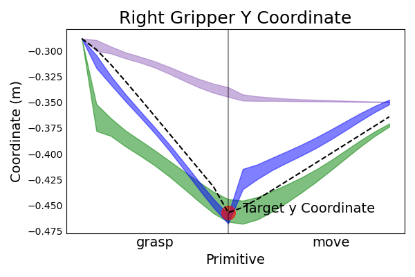
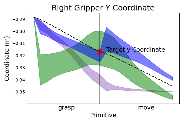
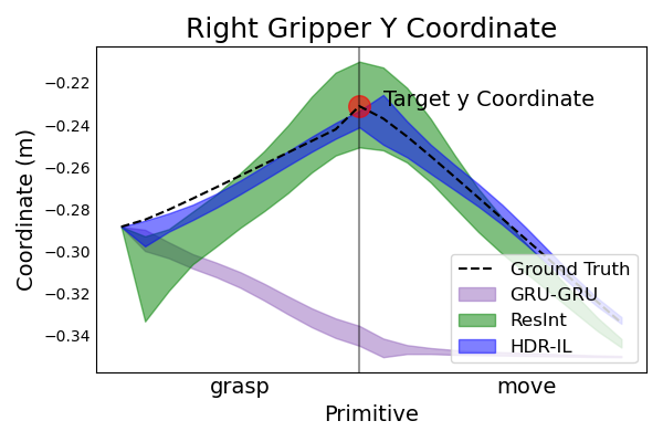
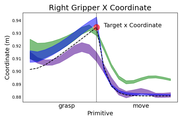
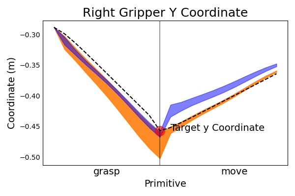
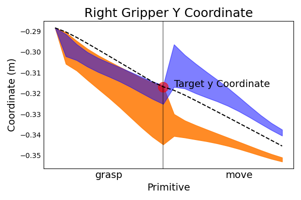
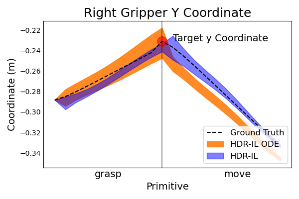
Figure 4 visualizes the predictions against the ground truth for the right gripper at the most critical grasp and move primitives. The left gripper follows a similar pattern. We pick the y-coordinates because they have the largest variability in the training demonstrations. The baseline models which did not have a graph structure or skip connections did not generalize well to changes in the table location and project roughly an average of the training trajectories. The ResInt model shows the ability to reach the target, while using multiple models helps to improve upon the precision of the generalizations further.

An alternative method to model object interactions is to use relational coordinates instead of absolute coordinates in the simulation data. We found the use of absolute data and graph structures performs better than using relational data. Combined with the skip connections, the absolute data and graphs performed significantly better in all metrics as shown in Table 2.

We even found our prediction from the HDR-ILmodel can achieve success for table starting locations where the ground truth demonstration failed. There were some failures ($<0.7\%$ of 2500 demonstrations) due to the approximations of the IK solver sometimes creating unusual movements between arm states. This causes the table to be dropped, which alters the arm trajectories in these demonstrations. Our model can account for these uncertainties in demonstration because of the stochastic sampling design shown in Figure 2.

Figure 4: Sample y coordinate predictions for 3 sample demonstrations in the table lifting task. The robot gripper reaches for the table leg, denoted by the "Target", whose location is randomized for each demonstration. The ResInt model has improved ability to generalize, compared to the baseline GRU-GRU model which tends to project an average trajectory over all training demos. The HDR-IL, which uses multiple dynamics models instead of a single model, improves the precision even more.

Table 2: Comparison of model performance between relational data versus absolute data. Absolute data with graphs to measure interactions performs significantly better than relational data when combined with the skip connection.

Model	Graph	Skip Conn	Relational	Euclidean Dist	Angular Dist	DTW Dist	% Success
GRU-GRU				$6.53\pm 7.05$	$0.139\pm 0.182$	0.135	13%
Res Relational		✓	✓	$8.15\pm 4.71$	$0.171\pm 0.153$	0.133	16%
ResInt	✓	✓		$5.64\pm 5.17$	$0.121\pm 0.205$	0.128	72%

(a) Phase 1: Aligning left table

(b) Phase 2: Aligning right table

(c) Phase 3: Combine and lift

Figure 5: Trajectories of gripper $xyz$ coordinates in the peg-in-hole task. Top row summarizes the actions taking place in 3 phases. The black dot in the 3D figure represents the starting point. The letters correspond to the bottom images. Lift success for this task is defined as both tables elevated evenly above ground, which can only be achieved if the two tables are connected.

5.3 Peg-in-Hole Task

Task Design

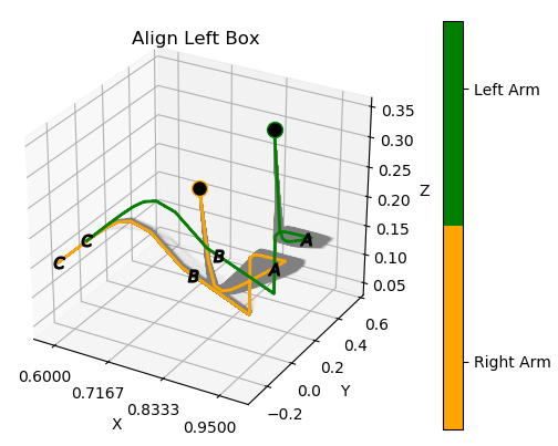
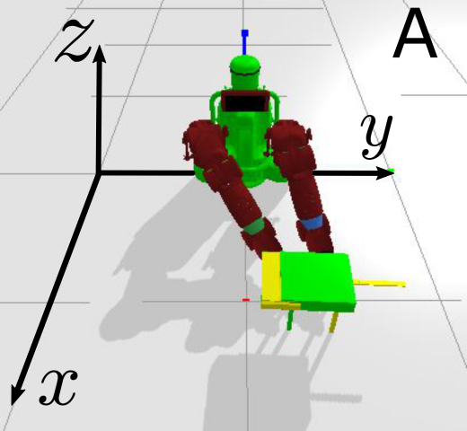
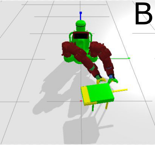
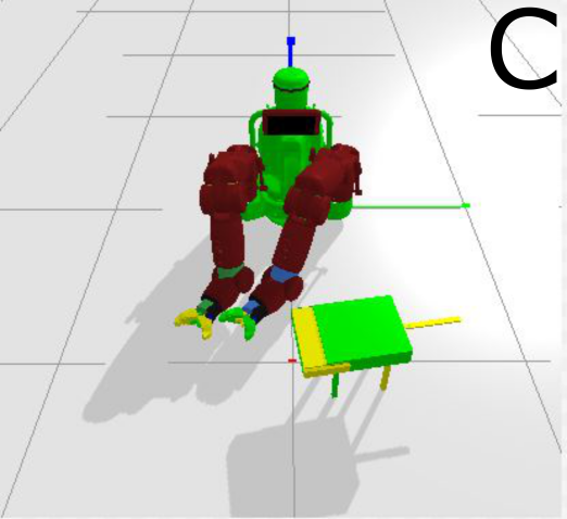
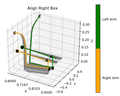
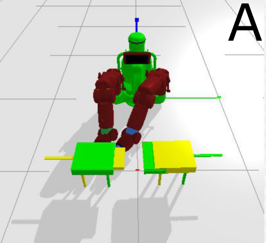
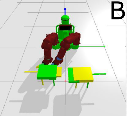
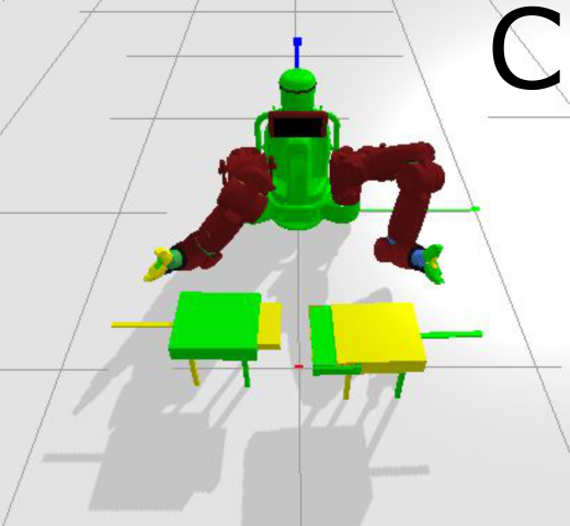
We evaluate the same models on a more difficult peg-in-hole task. The environment uses two tables, each measuring 35cm by 42.5cm. One table has a peg that needs to fit into the hole of the other table. To lift the tables off the ground, the robot first needs to precisely align and attach the two tables together, as illustrated in Figure 5. The tables start in random locations within their own 20cm by 20cm range. This task introduces three location generalizations, one for the location of each table and one in the location when combining and lifting the joined tables. Videos of the demonstrations are provided in the supplementary material.

Model Training

The model training follows the same strategy as the table lift task, using a total of 4700 demonstrations, each of length 130, with 13 primitives each of length 10. We trained with a batch size of 130 for 18,800 epochs and tested on a random sample of 281 starting points.

Results

The results in Table 3 shows our ResInt and HDR-IL model improved success rates compared to the GRU-GRU baseline model. Model success rates were lower across all of the models compared to the table lifting task due to the difficulty of the task. Average Euclidean distance errors are smaller because the range of table starting locations were smaller. The predictions usually fail in phase 2 due to lower accuracy in later time steps.

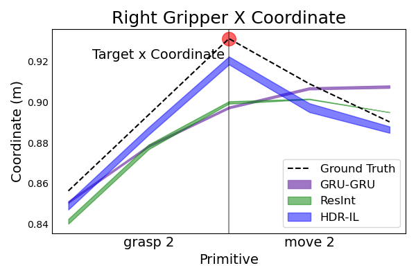
Generalizations along the x-axis were more difficult for this task due to larger variances in the demonstrations. Figure 6 compares the x-axis coordinate predictions at two different time windows for a single demo. In the time window of the first generalization (a), the HDR-IL and ResInt models are comparable in their generalization. They are both able to reach the target coordinate, shown as a red circle. The second time window (b) corresponding to the generalization in Phase 2 which is the around 60 time steps into task sequence. The HDR-IL model shows better generalization compared to the other two models, but it does not reach the target exactly. The decreased accuracy in the second and the third generalizations led to lower success rates in our simulations for all models.

(a) Phase 1 grasp table

(b) Phase 2 grasp table

Figure 6: X coordinate predictions comparison for two phases. (a) the HDR-IL and ResInt models are comparable in their generalization, both reaching the target coordinate, shown as a red circle. (b) 60 time steps into task sequence. HDR-IL shows better generalization compared to the other two models, but it does not reach the target exactly. The decreased accuracy in the second and the third generalizations led to lower success rates in our simulations for all models.

Table 3: Comparison of model performances in the peg-in-hole task. Euclidean distances errors are averages of the two grippers, and the ranges are one standard deviation. Angular distance measures the mean and standard deviation of the geodesic distance between the predicted and actual quaternions. The success rates are lower across all models in the task due to the more difficult task, which is both longer and requires more generalizations. Percent success was measured on 281 test simulations.

Model	Eculidean Dist	Angular Dist	DTW Dist	% Success - Lift
GRU-GRU	$2.11\pm 1.11$	$0.029\pm 0.022$	0.121	1%
ResInt	$1.59\pm 0.83$	$0.024\pm 0.012$	0.117	15%
HDR-IL	$0.90\pm 1.01$	$0.013\pm 0.010$	0.113	29%

6 Conclusion and Future Work

We present a novel deep imitation learning framework for learning complex control policies in bimanual manipulation tasks. This framework introduces a two-level hierarchical model for primitive selection and primitive dynamics modeling, utilizing graph structures and residual connections to model object dynamics interactions. In simulation, our model shows promising results on two complex bimanual manipulation tasks: table lifting and peg-in-hole. Future work include estimating object pose directly from visual inputs. Another interesting direction is automatic primitive discovery, which would greatly improve the label efficiency of training the model in new tasks.

Broader Impact

Robotics systems that utilize fully automated policies for different tasks have already been applied to many manufacturing, assembly lines, and warehouses processes. Our work demonstrates the potential to take this automation one step further. Our algorithm can automatically learn complex control policies from expert demonstrations, which could potentially allow robots to augment their existing control designs and further optimize their workflows. Implementing learned policies in safety-critical environments such as large-scale assembly lines can be risky as these algorithms do not have guaranteed precision. Improved theoretical understanding and interpretability of model policies could potentially mitigate these risks.

Appendix A Model Details

A.1 Model Parameters

The Hyper-parameters we tested and the best parameter we selected for each model.

Table 4: Summary of model hyperparameters tested in hyperparameter search and the value used in the final model.

Table Lift Task
Model	Parameters Searched	Planning Model	Dynamics Model - Single	Dynamics Model - Multi
Encoder LR	$2\times 10^{-4}$ - $1\times 10^{-5}$	$5\times 10^{-5}$	$2\times 10^{-4}$	$1\times 10^{-5}$
Decoder LR	$2\times 10^{-4}$ - $1\times 10^{-5}$	$5\times 10^{-5}$	$4\times 10^{-5}$	$4\times 10^{-5}$
Hidden Dimensions	100 - 1024	512	512	512
Encoder FC Layers	3-18	3	18	3
Decoder FC Layers	3-19	4	19	5
GAT attention layers	1, 2	1	1	1
Peg-In-Hole Task
Model	Parameters Searched	Planning Model	Dynamic Model - Single	Dynamic Model - Multi
Encoder LR	$2\times 10^{-4}$ - $1\times 10^{-5}$	$1\times 10^{-5}$	$5\times 10^{-5}$	$5\times 10^{-5}$
Decoder LR	$2\times 10^{-4}$ - $8\times 10^{-7}$	$8\times 10^{-7}$	$5\times 10^{-5}$	$5\times 10^{-5}$
Hidden Dimensions	100 - 1024	512	1024	512
Encoder FC Layers	3-20	9	20	3
Decoder FC Layers	3-21	8	21	5
GAT attention layers	1, 2	1	1	1
GAT attention heads	1, 2	1	1	1

A.2 Data Pre-processing

For the table lift task, we used 2,500 training demonstrations, with starting locations distributed uniformly over displacement range of 20cm by 60 cm. The testing was done on 127 random starting locations with displacements within the range of the training dataset. For the peg-in-hole task we used 4,700 randomly selected demonstrations for training and 281 random locations for testing. In data pre-processing, we removed demonstrations that were not successful in completing the tasks.

A.3 Dynamic Model Details

A.3.1 Encoder

Figure 7: Encoder training set-up details with graph structure and skip connection.

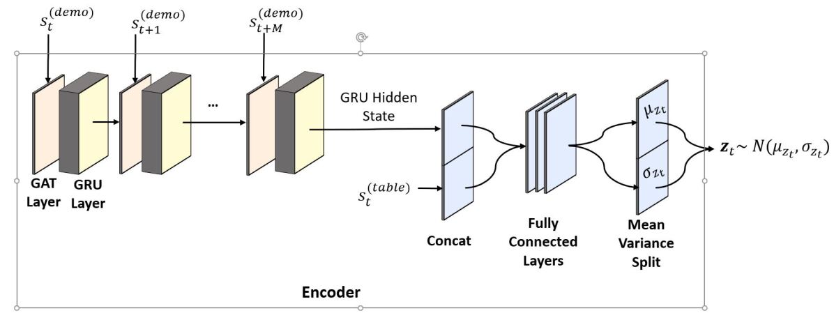
The baseline encoder consists of a GRU which takes the initial state as the input. The number of layers in the GRU corresponds to the number of states being projected. The initial state is a vector consisting of the $x$-, $y$-, and $z$-coordinates of each object concatenated with the quaternions for that object. During training, we use teacher forcing so that the input in each layer of the GRU take the states from the simulation. During testing, the inputs in layers besides the first come from the output of the previous layer. The hidden state of the GRU at the last time point is passed through the fully connected layers. The number of fully connected layers vary based on whether the model is part of a multi-model framework as outlined in the Model Parameters section. We modified the number of linear layers such that our single and multi-model designs have comparable number of parameters. The final layer doubles the dimensionality of the fully connected layers, splitting the hidden state into mean and variances for the decoder.

Relational Model Int

Models that use relational features use graph attention layers (GAT). We use one attention head in the GAT layers.

A node corresponds to an object feature in the state, one node for each of the x, y, z coordinates and for the four quaternions. We will index the layer with a superscript. The initial node feature $h_{u}^{(0)}$ is the value of that feature. For each layer, the edge attention coefficient $e_{uv}^{l}$ between nodes $u$ and $v$ is given by

$$e_{uv}^{(l)}=a\left(\mathbf{W}^{(l)}h_{u}^{(l)},\mathbf{W}^{(l)}h_{v}^{(l)}\right)$$ (1)

for learned layer weight matrix $\mathbf{W}^{(l)}$. The attention mechanism $a$ concatenates the inputs and multiplies them by a learned weight vector $\mathbf{a}^{(l)}$ and applies a nonlinearity, i.e.

$$e_{uv}^{(l)}=\mathrm{LeakyReLU}\left(\mathbf{a}^{(l)}(\mathbf{W}^{(l)}h_{u}^{(l)}||\mathbf{W}^{(l)}h_{v}^{(l)})\right)$$ (2)

Attention weights are computed by normalizing edge attention coefficients with the softmax function

$$\alpha_{uv}=\mathrm{softmax}(e_{uv}).$$ (3)

Node features are aggregated by neighborhood. For node $u$ and the set of its connected neighbors $\mathcal{N}_{u}$, node features are updated by the GAT update rule,

$$h^{(l+1)}_{u}=\sum_{v\in\mathcal{N}_{u}}\alpha\mathbf{W}^{(l)}h_{v}^{(l)}.$$ (4)

Figure 8: A graphical visualization of the attention weights learned in the 2nd layer of the GRU for the table lifting task. Node colors represent different objects in the environment. In this graph, ’R’ and ’L’ stand for left and right grippers, and ’T’ for table. The visible edges are those with attention weights greater than 8%. A graph convolution network (GCN) without learned weights would assume uniform attention weights of 4.77% for all 21 nodes. This supported our decision to use GAT over GCN for modeling the interactions. The two nodes receiving the largest weights are the right gripper y coordinate and a quaternion on the left gripper.

Residual Connection Res

Models that have the residual connection concatenate the table features to the final hidden state from the GRU, prior to the linear layers.

A.3.2 Decoder

Figure 9: Decoder training set-up details.

The decoder takes a sample latent space from the encoder. The sample is the initial hidden state going into the GRU of the decoder. The initial input of the first layer is a tensor of zeros. In the remaining layers, the input to the layer is the output from the previous layer. At each layer, the output of the GRU goes through a series of fully connected layers to get the final output of the model which represent the states at each time point.

ODE Model

In the ODE model, the latent state is passed to the ODE Solver, which replaces the GRU. The ODE solver solves for the time invariant gradient function, which used to generate the output at each time step.

A.4 Planning Model Details

Figure 10: Planning Models take a sequence of observed states and determines a primitive for the next step. The encoder setup is the same as the dynamics model, with the graph structure but no skip connection. The latent state in fixed rather than a distribution in the dynamic model. In the decoder, the output of the GRU and fully connected layers are fed through an additional softmax layer to get the primitive label.

Appendix B Additional Results

Figure 11: RNN vs ODE Model Introducing continuous time dynamics through the ODE model did not improve upon the predictions. This is due to the transitions of different primitives in this task being discrete.

Table 5: Breakdown of average Euclidean distance (cm) by primitives of table lift task. Errors are one standard deviation. The errors are the largest in the lift primitive because this primitive has the largest distances between time steps. The larger movements between time steps results in less precision in the predictions

Model	Grasp	Move	Lift	Extend	Place	Retract
GRU-GRU	$7.03\pm 5.45$	$9.34\pm 6.59$	$2.67\pm 1.66$	$14.20\pm 9.94$	$4.65\pm 2.91$	$1.39\pm 0.39$
Res	$8.33\pm 5.64$	$9.62\pm 6.69$	$4.44\pm 1.35$	$13.90\pm 7.74$	$5.30\pm 0.75$	$4.94\pm 1.41$
Int	$7.73\pm 5.20$	$9.66\pm 6.37$	$3.44\pm 1.19$	$12.57\pm 6.91$	$4.23\pm 2.40$	$2.61\pm 0.71$
ResInt	$3.80\pm 1.89$	$3.28\pm 1.36$	$3.87\pm 1.55$	$13.46\pm 8.09$	$5.72\pm 2.34$	$3.45\pm 0.69$
GRU-GRU Multi	$7.03\pm 5.45$	$9.35\pm 6.59$	$2.68\pm 1.65$	$14.20\pm 9.94$	$4.65\pm 2.92$	$1.40\pm 0.38$
Res Multi	$3.76\pm 1.63$	$3.59\pm 1.49$	$3.09\pm 1.87$	$13.53\pm 9.62$	$4.08\pm 2.22$	$1.54\pm 0.61$
Int Multi	$10.99\pm 9.20$	$10.01\pm 8.05$	$3.35\pm 2.34$	$18.04\pm 10.42$	$6.94\pm 4.24$	$20.68\pm 10.78$
HDR-IL	$2.86\pm 1.51$	$3.29\pm 1.34$	$2.98\pm 1.87$	$12.78\pm 8.71$	$3.73\pm 2.85$	$4.03\pm 0.85$

Table 6: Breakdown of average Euclidean distance (cm) by phase for the peg-in-hole task. Errors are one standard deviation.

Model	Phase 1	Phase 2	Phase 3
GRU-GRU	$1.89\pm 1.08$	$2.51\pm 1.22$	$1.79\pm 0.67$
ResInt	$1.93\pm 0.85$	$1.49\pm 0.86$	$1.18\pm 0.42$
HDR-IL	$1.45\pm 1.24$	$1.79\pm 1.30$	$1.29\pm 0.66$

Appendix C Simulations

All tasks used to train and test our framework were designed using the PyBullet physics simulator. Our goal when designing tasks was two-fold:

• Design tasks that could be easily decomposed into a sequence of simpler, low-level primitives.

• Design tasks that could not be performed using only one arm, and thus would fall under the domain of bimanual manipulation.

Task Design

Designing both tasks used for our experiments followed the same process. We first decided which low-level primitives the task should be decomposed into. Then we manually coded the primitives required and put them together sequentially. We made sure that if the robot used only one arm for either of the tasks it would fail, to ensure that learning to do the task successfully required true bimanual manipulation. We used the final position of the center of mass of the table or tables to measure task success.

Primitive Design

The process of designing the primitives was iterative. We first built the primitive movements and test them on the simulation of the task with the table at various starting locations and observe the performance and success rates. We observe where the simulations failed and adjust the primitives parameters as necessary. This including modifying the number of time steps and the trajectory of the primitive to avoid accidental interactions. All code used for our simulations will be made publicly available.

Datasets

All data was collected using the two scripts designed for the place-and-lift and peg-in-hole tasks. Both tasks had noise introduced to them in order to make the training data more robust. Our code is included to run our simulations and generate datasets.

References

- [1] Sanjay Krishnan, Roy Fox, Ion Stoica, and Ken Goldberg. Ddco: Discovery of deep continuous options for robot learning from demonstrations, 2017.
- [2] P. Pastor, H. Hoffmann, T. Asfour, and S. Schaal. Learning and generalization of motor skills by learning from demonstration. In 2009 IEEE International Conference on Robotics and Automation, pages 763–768, 2009.
- [3] A. Pervez, Y. Mao, and D. Lee. Learning deep movement primitives using convolutional neural networks. In 2017 IEEE-RAS 17th International Conference on Humanoid Robotics (Humanoids), pages 191–197, 2017.
- [4] T. Welschehold, C. Dornhege, and W. Burgard. Learning mobile manipulation actions from human demonstrations. In 2017 IEEE/RSJ International Conference on Intelligent Robots and Systems (IROS), pages 3196–3201, 2017.
- [5] Christian Smith, Yiannis Karayiannidis, Lazaros Nalpantidis, Xavi Gratal, Peng Qi, Dimos V Dimarogonas, and Danica Kragic. Dual arm manipulation—a survey. Robotics and Autonomous systems, 60(10):1340–1353, 2012.
- [6] Stefan Schaal. Learning from demonstration. In Neural Information Processing Systems, 1997.
- [7] Brenna D. Argall, Sonia Chernova, Manuela Veloso, and Brett Browning. A survey of robot learning from demonstration. Robotics and Autonomous Systems, 57(5):469–483, 2009.
- [8] Takayuki Osa, Joni Pajarinen, Gerhard Neumann, J Andrew Bagnell, Pieter Abbeel, Jan Peters, et al. An algorithmic perspective on imitation learning. Foundations and Trends® in Robotics, 7(1-2):1–179, 2018.
- [9] Chelsea Finn, Tianhe Yu, Tianhao Zhang, Pieter Abbeel, and Sergey Levine. One-shot visual imitation learning via meta-learning. In Conference on Robot Learning, 2017.
- [10] T. Zhang, Z. McCarthy, O. Jow, D. Lee, X. Chen, K. Goldberg, and P. Abbeel. Deep imitation learning for complex manipulation tasks from virtual reality teleoperation. In IEEE International Conference on Robotics and Automation, 2018.
- [11] Richard S Sutton, Doina Precup, and Satinder Singh. Between mdps and semi-mdps: A framework for temporal abstraction in reinforcement learning. Artificial intelligence, 112(1-2):181–211, 1999.
- [12] Milos Hauskrecht, Nicolas Meuleau, Leslie Pack Kaelbling, Thomas L Dean, and Craig Boutilier. Hierarchical solution of markov decision processes using macro-actions. arXiv preprint arXiv:1301.7381, 2013.
- [13] Bruno Da Silva, George Konidaris, and Andrew Barto. Learning parameterized skills. arXiv preprint arXiv:1206.6398, 2012.
- [14] Warwick Masson, Pravesh Ranchod, and George Konidaris. Reinforcement learning with parameterized actions. In Thirtieth AAAI Conference on Artificial Intelligence, 2016.
- [15] Matthew J. Hausknecht and Peter Stone. Deep reinforcement learning in parameterized action space. In 4th International Conference on Learning Representations, ICLR 2016, San Juan, Puerto Rico, May 2-4, 2016, Conference Track Proceedings, 2016.
- [16] Maciej Klimek, Henryk Michalewski, Piotr Mi, et al. Hierarchical reinforcement learning with parameters. In Conference on Robot Learning, pages 301–313, 2017.
- [17] Ermo Wei, Drew Wicke, and Sean Luke. Hierarchical approaches for reinforcement learning in parameterized action space. In 2018 AAAI Spring Symposium Series, 2018.
- [18] Jiechao Xiong, Qing Wang, Zhuoran Yang, Peng Sun, Lei Han, Yang Zheng, Haobo Fu, Tong Zhang, Ji Liu, and Han Liu. Parametrized deep q-networks learning: Reinforcement learning with discrete-continuous hybrid action space. arXiv preprint arXiv:1810.06394, 2018.
- [19] Oliver Kroemer, Christian Daniel, Gerhard Neumann, Herke Van Hoof, and Jan Peters. Towards learning hierarchical skills for multi-phase manipulation tasks. In 2015 IEEE International Conference on Robotics and Automation (ICRA), pages 1503–1510. IEEE, 2015.
- [20] Peter Pastor, Heiko Hoffmann, Tamim Asfour, and Stefan Schaal. Learning and generalization of motor skills by learning from demonstration. In 2009 IEEE International Conference on Robotics and Automation, pages 763–768. IEEE, 2009.
- [21] Simon Manschitz, Jens Kober, Michael Gienger, and Jan Peters. Learning movement primitive attractor goals and sequential skills from kinesthetic demonstrations. Robotics and Autonomous Systems, 74:97–107, 2015.
- [22] Rohan Chitnis, Shubham Tulsiani, Saurabh Gupta, and Abhinav Gupta. Efficient bimanual manipulation using learned task schemas. arXiv preprint arXiv:1909.13874, 2019.
- [23] Roy Fox, Richard Shin, William Paul, Yitian Zou, Dawn Song, Ken Goldberg, Pieter Abbeel, and Ion Stoica. Hierarchical variational imitation learning of control programs. arXiv preprint arXiv:1912.12612, 2019.
- [24] Andrej Gams, Aleš Ude, Jun Morimoto, et al. Deep encoder-decoder networks for mapping raw images to dynamic movement primitives. In 2018 IEEE International Conference on Robotics and Automation (ICRA), pages 1–6. IEEE, 2018.
- [25] M Yunus Seker, Mert Imre, Justus Piater, and Emre Ugur. Conditional neural movement primitives. In Robotics: Science and Systems (RSS), 2019.
- [26] Tianhe Yu, Pieter Abbeel, Sergey Levine, and Chelsea Finn. One-shot hierarchical imitation learning of compound visuomotor tasks. arXiv preprint arXiv:1810.11043, 2018.
- [27] Hoang M Le, Nan Jiang, Alekh Agarwal, Miroslav Dudík, Yisong Yue, and Hal Daumé. Hierarchical imitation and reinforcement learning. In 35th International Conference on Machine Learning, ICML 2018, pages 4560–4573. International Machine Learning Society (IMLS), 2018.
- [28] Thomas Kipf, Yujia Li, Hanjun Dai, Vinicius Zambaldi, Alvaro Sanchez-Gonzalez, Edward Grefenstette, Pushmeet Kohli, and Peter Battaglia. Compile: Compositional imitation learning and execution. In International Conference on Machine Learning, pages 3418–3428, 2019.
- [29] Kuan Fang, Yuke Zhu, Animesh Garg, Silvio Savarese, and Li Fei-Fei. Dynamics learning with cascaded variational inference for multi-step manipulation. arXiv preprint arXiv:1910.13395, 2019.
- [30] Franco Scarselli, Marco Gori, Ah Chung Tsoi, Markus Hagenbuchner, and Gabriele Monfardini. The graph neural network model. IEEE Transactions on Neural Networks, 20(1):61–80, 2008.
- [31] Thomas Kipf, Ethan Fetaya, Kuan-Chieh Wang, Max Welling, and Richard Zemel. Neural relational inference for interacting systems. arXiv preprint arXiv:1802.04687, 2018.
- [32] Damian Mrowca, Chengxu Zhuang, Elias Wang, Nick Haber, Li F Fei-Fei, Josh Tenenbaum, and Daniel L Yamins. Flexible neural representation for physics prediction. In S. Bengio, H. Wallach, H. Larochelle, K. Grauman, N. Cesa-Bianchi, and R. Garnett, editors, Advances in Neural Information Processing Systems 31, pages 8799–8810. Curran Associates, Inc., 2018.
- [33] Guangxiang Zhu, Zhiao Huang, and Chongjie Zhang. Object-oriented dynamics predictor. In Advances in Neural Information Processing Systems, pages 9804–9815, 2018.
- [34] Thomas Kipf, Elise van der Pol, and Max Welling. Contrastive learning of structured world models. In International Conference on Learning Representations, 2019.
- [35] Tingwu Wang, Renjie Liao, Jimmy Ba, and Sanja Fidler. Nervenet: Learning structured policy with graph neural networks. In International Conference on Learning Representations, 2018.
- [36] Ilya Sutskever, Oriol Vinyals, and Quoc V Le. Sequence to sequence learning with neural networks. In Advances in neural information processing systems, pages 3104–3112, 2014.
- [37] Nicholas Rhinehart, Rowan McAllister, and Sergey Levine. Deep imitative models for flexible inference, planning, and control, 2018.
- [38] Diederik P Kingma and Max Welling. Auto-encoding variational bayes. arXiv preprint arXiv:1312.6114, 2013.
- [39] Petar Veličković, Guillem Cucurull, Arantxa Casanova, Adriana Romero, Pietro Liò, and Yoshua Bengio. Graph attention networks. In International Conference on Learning Representations, 2018.
- [40] Kyunghyun Cho, Bart van Merrienboer, Dzmitry Bahdanau, and Yoshua Bengio. On the properties of neural machine translation: Encoder-decoder approaches, 2014.
- [41] YuXuan Liu, Abhishek Gupta, Pieter Abbeel, and Sergey Levine. Imitation from observation: Learning to imitate behaviors from raw video via context translation, 2017.
- [42] Erwin Coumans and Yunfei Bai. Pybullet, a python module for physics simulation for games, robotics and machine learning. http://pybullet.org, 2016–2019.