On the modified fractional Korteweg-de Vries and related equations

Abstract.

We consider in this paper modified fractional Korteweg-de Vries and related equations (modified Burgers-Hilbert and Whitham). They have the advantage with respect to the usual fractional KdV equation to have a defocusing case with a different dynamics. We will distinguish the weakly dispersive case where the phase velocity is unbounded for low frequencies and tends to zero at infinity and the strongly dispersive case where the phase velocity vanishes at the origin and goes to infinity at infinity. In the former case, the nonlinear hyperbolic effects dominate for large data, leading to the possibility of shock formation though the dispersive effects manifest for small initial data where scattering is possible. In the latter case, finite time blow-up is possible in the focusing case but not the shock formation. In the defocusing case global existence and scattering is expected in the energy subcritical case, while finite time blow-up is expected in the energy supercritical case.

We establish rigorously the existence of shocks with blow-up time and location being explicitly computed in the weakly dispersive case, while most of the results on the strongly dispersive case are derived via numerical simulations, for large solutions. Moreover, the shock formation result can be extended to the weakly dispersive equation with some generalized nonlinearity.

We will also comment briefly on the BBM versions of those equations.

1. Introduction

We consider the modified fractional Korteweg-de Vries (modified fKdV) equation

$$u_{t}\pm u^{2}u_{x}-|D|^{\alpha}\partial_{x}u=0,$$ (1.1)

where $D=-\mathrm{i}\partial_{x}$ and hence $|D|^{\alpha}$ has Fourier multiplier $|\xi|^{\alpha}$. We will distinguish the ”weakly dispersive” case $-1\leq\alpha<0$ and the ”strongly dispersive case $0<\alpha<2$. (We exclude the case $\alpha=2$ that corresponds to the well-known modified KdV equation.) Note that $\alpha=-1$ corresponds to the modified Burgers-Hilbert equation and $\alpha=1$ to the modified Benjamin-Ono equation.

The $+$ sign will be referred to as the focusing case and the $-$ sign as the defocusing case (actually this distinction is irrelevant when $\alpha<0$). It is well-known in the weakly dispersive case that the symbol $|D|^{\alpha}\partial_{x}$ has the expression

$$|D|^{\alpha}\partial_{x}f(x)=c_{\alpha}\int_{\mathbb{R}}\frac{\mathrm{sgn}(y)}{|y|^{2+\alpha}}[f(x)-f(x-y)]\,dy,$$

where $c_{\alpha}$ is a positive constant only depending on $\alpha$, which will be regarded as $1$ for simplicity.

The motivation of the present paper is, as in previous works concerning perturbations of the Burgers equation [6, 7, 11, 18, 19, 23, 28] to study the influence of a relatively weak dispersive perturbation on the dynamics of a quasilinear hyperbolic equation. Do the hyperbolic properties (appearance of shocks, global entropy weak solutions) persist or on the contrary do dispersive effects dominate? Of course both those properties might persist in the same equation and conversely depending on the size of the initial data.

The situation is quite different for $-1<\alpha<0$ and $0<\alpha\leq 1$ as can be seen by looking at the phase velocity $c(\xi)=|\xi|^{\alpha}$ which is unbounded for low frequencies and goes to zero for large frequencies in the former case. One thus expects that the nonlinear hyperbolic aspects dominate (for large solutions) in the case $\alpha<0$.

On the other hand dispersive effects appear for small solutions and actually in the case $-1<\alpha<0$ the global existence and modified scattering for (1.1) with small initial data was studied in [28] leading to the following result in the focusing case:

Proposition 1.1 ([28]).

Let $\alpha\in(-1,0)$. Define the profile

$$f(t,x)=e^{-t|D|^{\alpha}\partial_{x}}u(t,x),$$

and the $Z$-norm

$$\|g\|_{Z}=\|(1+|\xi|)^{10}\widehat{g}(\xi)\|_{L^{\infty}_{\xi}}.$$

Assume that $N_{0}=100,\ p_{0}\in(0,\frac{1}{1000}]\cap(0,-\frac{\alpha}{100}]$ are fixed, and $\phi\in H^{N_{0}}(\mathbb{R})$ satisfies

$$\|\phi\|_{H^{N_{0}}}+\|\phi\|_{H^{1,1}}+\|\phi\|_{Z}=\varepsilon_{0}\leq\bar{\varepsilon},$$

for some constant $\bar{\varepsilon}$ sufficiently small (depending only on $\alpha$ and $p_{0}$). Then the Cauchy problem of the equation (1.1) with the initial data $u(0,x)=\phi(x)$ admits a unique global solution $u\in C(\mathbb{R}:H^{N_{0}}(\mathbb{R}))$ satisfying the following uniform bounds for $t\geq 1$

$$t^{-p_{0}}\|u\|_{H^{N_{0}}}+t^{-p_{0}}\|f\|_{H^{1,1}}+\|f\|_{Z}\lesssim\varepsilon_{0}.$$

Moreover, there exists $w_{\infty}\in L^{\infty}(\mathbb{R})$ such that for $t\geq 1$

$$t^{p_{0}}\left\|\exp\left(\frac{3\mathrm{i}\xi|\xi|^{1-\alpha}}{\alpha(\alpha+1)}\int_{1}^{t}|\widehat{f}(s,\xi)|^{2}\,\frac{ds}{s}\right)(1+|\xi|)^{10}\widehat{f}(\xi)-w_{\infty}(\xi)\right\|_{L^{\infty}_{\xi}}\lesssim\varepsilon_{0}.$$

One aim of the present paper is to prove that the solutions of the equation (1.1) can form shocks for large initial data. We recall that the fKdV equation

$$u_{t}+uu_{x}-|D|^{\alpha}u_{x}=0$$ (1.2)

can form shocks for large solutions in the range $\alpha\in(-1,-1/3)$ [9, 10, 29]. We will show a similar shock formation result holds true for the equation (1.1), but for the whole range $\alpha\in(-1,0)$ .

On the other hand, when $\alpha>0$ the dispersive effects play a more important role and although finite time blow-up is expected, it should not be shock formation (see for the quadratic case the numerics in [18] and the results on the local Cauchy problem in [19, 23, 22] where the dispersive properties are used to enlarge the space of resolution).

We go back to the cubic case and first comment on the case $\alpha>0.$ In addition to the conservation of the $L^{2}$ norm (mass), one has the (Hamiltonian) formally conserved quantity

$$H_{\alpha}(u)=\frac{1}{2}\int_{\mathbb{R}}\left(|D^{\alpha/2}u|^{2}\mp\frac{1}{6}u^{4}\right)\,dx,$$

which by the Sobolev embedding $H^{1/4}(\mathbb{R})\subset L^{4}(\mathbb{R})$ implies that $\alpha=1/2$ is the energy critical exponent. On the other hand, (1.1) is invariant under the scaling transformation $u_{\lambda}(x)=\lambda^{\alpha/2}u(\lambda x,\lambda^{\alpha+1}t)$ which implies that $\alpha=1$ is the $L^{2}$ critical exponent.

In the defocusing case and when $\alpha>0$ one has a formal conservation of the energy space $H^{\alpha/2}(\mathbb{R})$.

Thus one expects in the focusing case global well-posedness in the energy space when $\alpha>1$ and finite time blow-up when $0<\alpha\leq 1.$ Note that the case $\alpha=1$ corresponds to the modified Benjamin-Ono equation and the finite time blow-up in the focusing case has been proved by Martel and Pilod[21]. The blow-up should not be a shock (the sup-norm of the solution and of the derivative should blow up at the same time) but its structure should be different in the energy super critical case $0<\alpha<1/2$ and in the $L^{2}-$ critical case $1/2\leq\alpha<1$. Again we refer to [18] for numerical simulations in the quadratic case.

Concerning the local Cauchy problem in ”large” Sobolev spaces (that is larger than the ”hyperbolic space” $H^{3/2+}(\mathbb{R})$) we are not aware of results similar to those in [19, 23] corresponding to the quadratic space except when $\alpha=1$ (the modified Benjamin-Ono equation considered in [13, 15]). In particular it is proven in [15] that the Cauchy problem for the focusing and defocusing modified Benjamin-Ono equation is locally well-posed in $H^{s}(\mathbb{R}),s\geq 1/2$ and thus globally well-posed in the same range in the defocusing case. (The local well-posedness in $H^{1}(\mathbb{R})$ was proven in [13]).

In the defocusing case, while one expects global well-posedness (and scattering) in the energy subcritical case $\alpha\geq 1/2$, things are unclear in the energy supercritical case and one aim of this paper is to present relevant conjectures.

This is in contrast to the case $\alpha<0$ where the hyperbolic effects dominate for large solutions and the distinction between focusing and defocusing becomes irrelevant.

The paper is organized as follows: The first Section is devoted to the statement and the proof of the main result Theorem 2.1 in the case $-1<\alpha<0$, that is the possibility of shocks. In the next two Sections we extend the shock formation result to the modified Burgers-Hilbert and Whitham equations, and the fractional Korteweg-de Vries equation with some generalized nonlinearity. Then we focus on the case $\alpha>0$, and consider successively the solitary wave solutions and the Cauchy problem in the focusing and defocusing case. Most issues will lead to conjectures illustrated by numerical simulations.

We conclude the paper by some remarks on the ”BBM” version of the modified fKdV equation when $\alpha>0.$

2. The case $-1<\alpha<0.$

2.1. Main result

We say that the solution of (1.1) exhibits shock formation if there exists some $T>0$ such that

$$|u(x,t)|<\infty,\quad x\in\mathbb{R},\ t\in[0,T),$$

but

$$\sup_{x\in\mathbb{R}}|\partial_{x}u(x,t)|\longrightarrow+\infty,\quad\text{as}\ t\longrightarrow T-.$$

The main result of this Section is stated as follows in the focusing case :

Theorem 2.1.

(Rough version) Let $\alpha\in(-1,0)$. There exists a wide class of functions $\phi\in H^{3}(\mathbb{R})$ with appropriate large positive amplitude $\phi$ and negative slope $\inf_{x\in\mathbb{R}}\phi^{\prime}(x)$ such that the Cauchy problem for the equation (1.1) with initial data $u(0,x)=\phi(x)$ exhibits shock formation.

(Precise version) Let $\alpha\in(-1,0)$ and $\delta$ be a sufficiently small positive number. Assume $\bar{x}_{1}$ and $\bar{x}_{2}$ are the largest and smallest numbers such that $\overline{\{x:\phi^{\prime}(x)<0\}}\subset[\bar{x}_{1},\bar{x}_{2}]$. If $\phi\in H^{3}(\mathbb{R})$ satisfies the slope condition

$$-\inf_{x\in\mathbb{R}}\phi^{\prime}(x)>\delta^{-1}f_{1},$$ (2.1)

$$-\inf_{x\in\mathbb{R}}\phi^{\prime}(x)>(1-\delta)^{-2}f_{2},$$ (2.2)

$$-\inf_{x\in\mathbb{R}}\phi^{\prime}(x)>(1-\delta)^{-3}f_{3},$$ (2.3)

and the local amplitude condition

$$\phi(x)<B-(1-\delta)^{-2}f_{4},$$ (2.4)

$$\phi(x)>A+(1-\delta)^{-2}f_{4},$$ (2.5)

for all $x\in[\bar{x}_{1},\bar{x}_{2}]$. Here the functions $(f_{1},f_{2},f_{3},f_{4})$ are homogeneous in each argument of order $(1/2,0,0,0)$, and have the following explicit formulae

$$\quad f_{1}=:f_{1}(\|\phi\|_{H^{2}},C_{1},\|\phi^{\prime\prime\prime}\|_{L^{2}})$$

$$=\big{[}C_{s}\|\phi\|_{H^{2}}+4C_{1}(1+\alpha)^{-1}+2C_{s}(-\alpha)^{-1}(2^{-1}AB^{-1})^{-7BA^{-2}/4}\|\phi^{\prime\prime\prime}\|_{L^{2}}\big{]}^{1/2},$$

$$f_{2}=:f_{2}(C_{0}^{-1}C_{1})=8(-\alpha(1+\alpha))^{-1}+4\alpha^{-2}C_{0}^{-1}C_{1},$$

$$\quad f_{3}=:f_{3}(C_{1}^{-1}\|\phi^{\prime\prime\prime}\|_{L^{2}})$$

$$=8(1+\alpha)^{-1}+4C_{s}(-\alpha)^{-1}(2^{-1}AB^{-1})^{-7BA^{-2}/4}C_{1}^{-1}\|\phi^{\prime\prime\prime}\|_{L^{2}},$$

$$\quad f_{4}=:f_{4}\big{(}C_{0}\big{(}-\inf_{x\in\mathbb{R}}\phi^{\prime}(x)\big{)}^{-1},C_{1}\big{(}-\inf_{x\in\mathbb{R}}\phi^{\prime}(x)\big{)}^{-1}\big{)}$$

$$=\big{(}-\inf_{x\in\mathbb{R}}\phi^{\prime}(x)\big{)}^{-1}\big{[}4C_{0}\big{(}-\alpha(1+\alpha)\big{)}^{-1}+2C_{1}\alpha^{-2}\big{]},$$

where $C_{0}>0$ and $C_{1}>0$ satisfying

$$\|\phi\|_{L^{\infty}}\leq\frac{C_{0}}{2},\quad\|\phi^{\prime}\|_{L^{\infty}}\leq\frac{C_{1}}{2},$$ (2.6)

and $A>0$ and $B>0$ satisfying

$$A^{2}>8\delta B^{2},\quad 8A^{2}>7B,\quad B>A+2(1-\delta)^{-2}f_{4},$$ (2.7)

and $C_{s}$ is the best embedding constant of Sobolev inequality

$$\|f\|_{L^{\infty}(\mathbb{R})}\leq C_{s}\|f\|_{H^{1}(\mathbb{R})}.$$

Then the solution for the equation (1.1) with initial data $u(0,x)=\phi(x)$ exhibits shock formation at some time $T>0$ satisfying

$$(2B+\delta)^{-1}\big{(}-\inf_{x\in\mathbb{R}}\phi^{\prime}(x)\big{)}^{-1}<T$$ (2.8)

$$<(AB^{-1}-\delta)^{-1}(2A-\delta)^{-1}\big{(}-\inf_{x\in\mathbb{R}}\phi^{\prime}(x)\big{)}^{-1},$$

and at some location $x_{*}$ satisfying

$$\bar{x}_{1}-C_{0}^{2}T\leq x_{*}\leq\bar{x}_{2}+C_{0}^{2}T.$$ (2.9)

Moreover, we have the blow-up rate estimate

$$(2B+\delta)^{-1}(T-t)^{-1}\leq\|\partial_{x}u(\cdot,t)\|_{L^{\infty}}\leq(AB^{-1}-\delta)^{-1}(2A-\delta)^{-1}(T-t)^{-1},$$ (2.10)

as $t\rightarrow T^{-}$.

Compared to the fKdV equation, the additional price for (1.1) that one shall pay is not only to assume the negative slope $\phi^{\prime}$ is appropriately large but also $\phi$ itself. The reason lies in that the nonlinear term $2v_{0}v_{1}^{2}$ (which is expected to be the leading term) of the equation (1.1) in particle path form (see (2.17)) has no fixed sign generally. To make sure that $v_{0}(t,x)=u(t,X(t,x))$ (see (2.12)) has a positive lower bound, we need to impose some kind of conditions such as (2.4)-(2.5) on $\phi$, and then verify that $v_{0}(t,x)$ is bounded below by a positive constant before the shock comes.

Remark 2.2.

There exists a wide class of functions $\phi\in H^{3}(\mathbb{R})$ satisfying (2.1)-(2.5) in Theorem 2.1. This can be seen easily from the orders of $\phi$ in both sides of each inequality by homogeneities of the functions $(f_{1},f_{2},f_{3},f_{4})$ on each of its arguments. Indeed, the left hand side of (2.1)-(2.5) has one more order on $\phi$ than that of the right hand side correspondingly, if the original $\phi$ does not work, then one can replace it by $\lambda\phi$ with a sufficiently large $\lambda>0$.

Remark 2.3.

There exists an open neighborhood in the $H^{3}$-topology of the set of initial data satisfying the hypotheses in Theorem 2.1 such that the conclusions of Theorem 2.1 hold. This is an obvious fact since the inequalities (2.1)-(2.5) are stable for small perturbations. So Theorem 2.1 contains the following precise information on the shock:
(a1) shock time;
(a2) shock location;
(a3) shock blow-up rate;
(a4) openness for initial data of producing shock.

Remark 2.4.

We emphasize that in the local amplitude condition (2.4)-(2.5), the interval $[\bar{x}_{1},\bar{x}_{2}]$ can be replaced by a larger but finite interval. Otherwise, the local amplitude condition will become a global one, which means $\phi\notin L^{2}(\mathbb{R})$ and thus contradicts $\phi\in H^{3}(\mathbb{R})$. More importantly, if the latter case happened, then $\phi$ is positive on the entire line which is physically irrelevant since $\phi$ stands for the initial elevation.

Remark 2.5.

We mention here previous works on the finite time blow-up phenomena for related weakly dispersive nonlinear equations. Naumkin and Shishmarev [25], and Constantin and Escher [4] have proven shock formation for a Whitham type equation which, however, does not include the Whitham equation considered in this paper. We now consider the fKdV equation (1.2) for $-1<\alpha<0$. The finite time blow-up of a $C^{1+\delta}(\mathbb{R})$ norm was established in [3] but the shock formation was not proven there. The possibility of appearance of shocks was proven in [9, 10] when $-1<\alpha<-1/3$ and for the Whitham equation. A simpler proof, applying to the case $-1<\alpha<-2/5$ and the Whitham equation was given in [29].

2.2. Proof of Theorem 2.1

It is standard (see e.g., [27]) to show that the Cauchy problem for the equation (1.1) with initial data $u(0,x)=\phi(x)$ is well-posed in the class $C([0,T):H^{3}(\mathbb{R}))$ for some $T>0$ which in what follows will denote the maximal time of existence.

We define the particle path

$$\frac{d}{dt}X(t,x)=u^{2}(t,X(t,x)),$$ (2.11)

$$X(0,x)=x.$$

Since $u(x,t)\in C([0,T):H^{3}(\mathbb{R}))$, the ODE theory shows that $X(\cdot;x)$ exists throughout the interval $t\in[0,T)$ for all $x\in\mathbb{R}$. We define

$$v_{0}(t,x)=u(t,X(t,x)),$$ (2.12)

$$v_{1}(t,x)=\partial_{x}u(t,X(t,x)),$$

and

$$m(t)=\inf_{x\in\mathbb{R}}v_{1}(t;x)=\inf_{x\in\mathbb{R}}\partial_{x}u(x,t)=:m(0)q^{-1}(t).$$ (2.13)

It is easy to see that

$$m(t)<0,\quad t\in[0,T),$$ (2.14)

$$q(0)=1,\quad q(t)>0,\quad t\in[0,T).$$ (2.15)

It then follows from (1.1) that

$$\frac{dv_{0}}{dt}+K_{0}(t,x)=0,$$ (2.16)

$$\frac{dv_{1}}{dt}+2v_{0}v_{1}^{2}+K_{1}(t,x)=0,$$ (2.17)

where

$$K_{0}(t,x)=\int_{\mathbb{R}}\frac{\mathrm{sgn}(y)}{|y|^{2+\alpha}}[u(t,X(t,x))-u(t,X(t,x)-y)]\,dy,$$ (2.18)

$$K_{1}(t,x)=\int_{\mathbb{R}}\frac{\mathrm{sgn}(y)}{|y|^{2+\alpha}}[\partial_{x}u(t,X(t,x))-\partial_{x}u(t,X(t,x)-y)]\,dy.$$ (2.19)

The main ingredient is to show

$$|K_{1}(t,x)|<\delta^{2}m^{2}(t),\quad\mathrm{for\ all}\ t\in[0,T)\ \mathrm{and}\ x\in\mathbb{R}.$$ (2.20)

In view of (2.1), one easily checks that (2.20) holds at $t=0$. We will prove (2.20) by contradiction. Suppose that $|K_{1}(T_{1},x_{0})|=\delta^{2}m^{2}(T_{1})$ for some $T_{1}\in(0,T)$ and some $x_{0}\in\mathbb{R}$. By continuity, without loss of generality, we may assume that

$$|K_{1}(t,x)|\leq\delta^{2}m^{2}(t),\quad\text{for\ all}\ t\in[0,T_{1}]\ \mathrm{and}\ x\in\mathbb{R}.$$ (2.21)

The following technical lemmas are a variant of those in [25, 9, 29] which dealt with the quadratic nonlinearity. Differently, here we need to work near the shock to deal with the cubic nonlinearity.

2.2.1. Bounds on $q(t)$

Let $t\in[0,T_{1}]$ and $x\in[\bar{x}_{1},\bar{x}_{2}]$. We a priori assume

$$A\leq v_{0}(t,x)\leq B,$$ (2.22)

in which $A$ and $B$ are given in Theorem 2.1 satisfying (2.7).

We define

$$\Sigma_{\delta}(t)=\{x\in[\bar{x}_{1},\bar{x}_{2}]:\ v_{1}(t,x)\leq(AB^{-1}-\delta)m(t)\},$$

and

$$v_{1}(t,x)=:m(0)r^{-1}(t,x).$$

Lemma 2.6.

We have $\Sigma_{\delta}(t_{2})\subset\Sigma_{\delta}(t_{1})$ whenever $0\leq t_{1}\leq t_{2}\leq T_{1}$.

Proof.

Suppose that there exists some $x_{1}\in[\bar{x}_{1},\bar{x}_{2}]$ such that $x_{1}\notin\Sigma_{\delta}(t_{1})$ but $x_{1}\in\Sigma_{\delta}(t_{2})$ for some $0\leq t_{1}\leq t_{2}\leq T_{1}$, that is

$$v_{1}(t_{1},x_{1})>(AB^{-1}-\delta)m(t_{1}),$$ (2.23)

$$v_{1}(t_{2},x_{1})\leq(AB^{-1}-\delta)m(t_{2})<\frac{1}{2}AB^{-1}m(t_{2}).$$

Since $v_{1}(\cdot,x_{1})$ and $m$ are uniformly continuous on $[0,T_{1}]$, due to the second inequality of (2.23), one can choose $t_{1}$ and $t_{2}$ sufficiently close so that

$$v_{1}(t,x_{1})\leq\frac{1}{2}AB^{-1}m(t),\quad\text{for\ all}\ t\in[t_{1},t_{2}].$$ (2.24)

Let

$$v_{1}(t_{1},x_{2})=m(t_{1})\big{(}\leq\frac{1}{2}AB^{-1}m(t_{1})\big{)},$$ (2.25)

again one may choose $t_{2}$ close to $t_{1}$ so that

$$v_{1}(t,x_{2})\leq\frac{1}{2}AB^{-1}m(t),\quad\text{for\ all}\ t\in[t_{1},t_{2}].$$ (2.26)

In the following we fix $t_{1}$ and $t_{2}$ such that all the inequalities (2.23), (2.24) and (2.26) hold true.

According to (2.21) and $A^{2}>8\delta B^{2}$ in (2.7), one has

$$|K_{1}(t,x_{j})|\leq\delta^{2}m^{2}(t)\leq 4A^{-2}B^{2}\delta^{2}v_{1}^{2}(t,x_{j})<\frac{\delta}{2}v_{1}^{2}(t,x_{j}),$$

for all $t\in[t_{1},t_{2}],\ j=1,2$. This together with (2.17) yields

$$\frac{dv_{1}}{dt}(t,x_{1}) =-2v_{0}v_{1}^{2}(t,x_{1})-K_{1}(t,x_{1})$$

$$\geq-\big{(}2v_{0}(t,x_{1})+\frac{\delta}{2}\big{)}v_{1}^{2}(t,x_{1}),$$

$$\geq-\big{(}2B+\frac{\delta}{2}\big{)}v_{1}^{2}(t,x_{1}),$$

and

$$\frac{dv_{1}}{dt}(t,x_{2}) =-2v_{0}v_{1}^{2}(t,x_{2})-K_{1}(t,x_{2})$$

$$\leq-\big{(}2v_{0}(t,x_{2})-\frac{\delta}{2}\big{)}v_{1}^{2}(t,x_{2}),$$

$$\leq-\big{(}2A-\frac{\delta}{2}\big{)}v_{1}^{2}(t,x_{2}),$$

for $t\in[t_{1},t_{2}]$. Solving the resulting two inequalities above gives

$$v_{1}(t_{2},x_{1})\geq\frac{v_{1}(t_{1},x_{1})}{1+\big{(}2B+\frac{\delta}{2}\big{)}v_{1}(t_{1},x_{1})(t_{2}-t_{1})},$$ (2.27)

and

$$v_{1}(t_{2},x_{2})\leq\frac{v_{1}(t_{1},x_{2})}{1+\big{(}2A-\frac{\delta}{2}\big{)}v_{1}(t_{1},x_{2})(t_{2}-t_{1})}.$$ (2.28)

Applying (2.25) to (2.28), one obtains

$$m(t_{2})\leq\frac{m(t_{1})}{1+\big{(}2A-\frac{\delta}{2}\big{)}m(t_{1})(t_{2}-t_{1})}.$$ (2.29)

In view of (2.23) and (2.27), one estimates

$$v_{1}(t_{2},x_{1}) >\frac{(AB^{-1}-\delta)m(t_{1})}{1+\big{(}2B+\frac{\delta}{2}\big{)}(AB^{-1}-\delta)m(t_{1})(t_{2}-t_{1})}$$

$$>\frac{(AB^{-1}-\delta)m(t_{1})}{1+\big{(}2A-\frac{\delta}{2}\big{)}m(t_{1})(t_{2}-t_{1})}$$

$$>(AB^{-1}-\delta)m(t_{2}),$$

where we have used (2.29) in the last inequality. We get a contradiction!

∎

Lemma 2.7.

$q(t)$ is decreasing and satisfies

$$0<q(t)\leq 1,\quad\text{for}\ t\in[0,T_{1}].$$ (2.30)

We also have the integral estimates

$$\int_{0}^{t}q^{-s}(\tau)\,d\tau \leq(1-s)^{-1}m^{-1}(0)(2A-\delta)^{-1}(AB^{-1}-\delta)^{-s}$$ (2.31)

$$\quad\times\big{[}q^{1-s}(t)-(AB^{-1}-\delta)^{s-1}\big{]},\quad\text{for}\ t\in[0,T_{1}].$$

where $s>0,s\neq 1$, and

$$\int_{0}^{t}q^{-1}(\tau)\,d\tau \leq m^{-1}(0)(2A-\delta)^{-1}(AB^{-1}-\delta)^{-1}$$ (2.32)

$$\quad\times\big{[}\log(AB^{-1}-\delta)+\log q(t)\big{]},\quad\text{for}\ t\in[0,T_{1}].$$

Proof.

Let $x\in\Sigma_{\delta}(T_{1})$, it first follows from Lemma 2.6 that

$$m(t)\leq v_{1}(t,x)\leq(AB^{-1}-\delta)m(t),\quad\text{for}\ t\in[0,T_{1}].$$ (2.33)

The solution of (2.17) can be expressed

$$m(0)r^{-1}(t,x)=v_{1}(t,x)$$ (2.34)

$$=\frac{v_{1}(0,x)}{1+v_{1}(0,x)\int_{0}^{t}\big{[}2v_{0}(\tau,x)+v_{1}^{-2}K_{1}(\tau,x)\big{]}\,d\tau}.$$

It follows from (2.21) and (2.33) that

$$|v_{1}^{-2}K_{1}(\tau,x)|\leq(AB^{-1}-\delta)^{-2}\delta^{2}<\delta,\quad\text{for}\ t\in[0,T_{1}]\ \text{and}\ x\in\Sigma_{\delta}(T_{1}).$$

This together with (2.34) implies

$$(2B+\delta)m(0)\leq\frac{d}{dt}r(t,x)\leq(2A-\delta)m(0),\quad\text{for}\ t\in[0,T_{1}]\ \text{and}\ x\in\Sigma_{\delta}(T_{1}).$$ (2.35)

It is easy to see that $r(t,x)$ is decreasing for all $t\in[0,T_{1}]$ from (2.35), and hence $v_{1}(t,x)$, too. Furthermore, by (2.13), $q(t)$ is also decreasing for all $t\in[0,T_{1}]$, which implies (2.30) by (2.15).

On the other hand, we conclude from (2.13), (2.33) and (2.34) that

$$q(t)\leq r(t,x)\leq(AB^{-1}-\delta)^{-1}q(t),\quad\text{for}\ t\in[0,T_{1}]\ \text{and}\ x\in\Sigma_{\delta}(T_{1}).$$ (2.36)

Let $s>0,s\neq 1$, we use (2.35) and (2.36) to deduce that

$$\int_{0}^{t}q^{-s}(\tau)\,d\tau\leq(AB^{-1}-\delta)^{-s}\int_{0}^{t}r^{-s}(\tau,x)\,d\tau$$

$$\leq m^{-1}(0)(2A-\delta)^{-1}(AB^{-1}-\delta)^{-s}\int_{0}^{t}r^{-s}(\tau,x)\frac{d}{d\tau}r(\tau,x)\,d\tau$$

$$=(1-s)^{-1}m^{-1}(0)(2A-\delta)^{-1}(AB^{-1}-\delta)^{-s}[r^{1-s}(t,x)-r^{1-s}(0,x)],$$

which combines (2.36) again implies (2.31). One can verify (2.32) similarly. ∎

To show (2.21), we also use a contradiction argument. We claim that

$$\|v_{0}(t)\|_{L^{\infty}}=\|u(t)\|_{L^{\infty}}<C_{0},\quad\text{for\ all}\ t\in[0,T_{1}],$$ (2.37)

and

$$\|v_{1}(t)\|_{L^{\infty}}=\|\partial_{x}u(t)\|_{L^{\infty}}<C_{1}q^{-1}(t),\quad\text{for\ all}\ t\in[0,T_{1}],$$ (2.38)

where $C_{0},C_{1}$ satisfy (2.6). First observe that

$$\|v_{0}(0)\|_{L^{\infty}}=\|\phi\|_{L^{\infty}}<C_{0},$$

and

$$\|v_{1}(0)\|_{L^{\infty}}=\|\phi^{\prime}\|_{L^{\infty}}<C_{1}q^{-1}(0).$$

We then proceed by contradiction in order to show (2.37) and (2.38). Suppose that (2.37) and (2.38) hold for all $t\in[0,T_{2})$, but fails for either (2.37) or (2.38) at $t=T_{2}$ for some $T_{2}\in(0,T_{1}]$. Hence, by continuity, it holds

$$\|v_{0}(t)\|_{L^{\infty}}=\|u(t)\|_{L^{\infty}}\leq C_{0},\quad\text{for\ all}\ t\in[0,T_{2}],$$ (2.39)

and

$$\|v_{1}(t)\|_{L^{\infty}}=\|\partial_{x}u(t)\|_{L^{\infty}}\leq C_{1}q^{-1}(t),\quad\text{for\ all}\ t\in[0,T_{2}].$$ (2.40)

2.2.2. Estimates on Nonlocal Terms

Lemma 2.8.

For all $t\in[0,T_{2}]$ and $x\in\mathbb{R}$, we have

$$|K_{0}(t,x)|\leq\big{[}4C_{0}(1+\alpha)^{-1}+2C_{1}(-\alpha)^{-1}\big{]}q(t)^{-(1+\alpha)},$$ (2.41)

and

$$|K_{1}(t,x)|\leq\big{[}4C_{1}(1+\alpha)^{-1}+2C_{s}(-\alpha)^{-1}(2^{-1}AB^{-1})^{-7BA^{-2}/4}\|\phi^{\prime\prime\prime}\|_{L^{2}}\big{]}q^{-2}(t),$$ (2.42)

Proof.

We follow the idea of [29], however the proof here is simpler when dealing with $\|\partial_{x}^{2}u\|_{L^{\infty}}$ in order to estimate $K_{1}(t,x)$ than that of the fKdV equation due to the stronger nonlinear effect present in the equation (1.1). The proof on $K_{0}(t,x)$ is the same as that of [29], we include it here for sake of completeness. To estimate the terms $K_{0}(t,x)$ and $K_{1}(t,x)$, we perform the following decompositions

$$|K_{0}(t,x)|\leq A_{1}+A_{2},$$

$$|K_{1}(t,x)|\leq B_{1}+B_{2},$$

where

$$A_{1}=\int_{|y|<\eta_{1}}\frac{1}{|y|^{2+\alpha}}\big{|}u(t,X(t,x))-u(t,X(t,x)-y)\big{|}\,dy,$$

$$A_{2}=\int_{|y|\geq\eta_{1}}\frac{1}{|y|^{2+\alpha}}\big{|}u(t,X(t,x))-u(t,X(t,x)-y)\big{|}\,dy,$$

$$B_{1}=\int_{|y|<\eta_{2}}\frac{1}{|y|^{2+\alpha}}\big{|}\partial_{x}u(t,X(t,x))-\partial_{x}u(t,X(t,x)-y)\big{|}\,dy,$$

$$B_{2}=\int_{|y|\geq\eta_{2}}\frac{1}{|y|^{2+\alpha}}\big{|}\partial_{x}u(t,X(t,x))-\partial_{x}u(t,X(t,x)-y)\big{|}\,dy,$$

for some $\eta_{1}>0$ and $\eta_{2}>0$ to be specified later. In view of (2.39)-(2.40), one may estimate

$$|A_{1}| \leq|u|_{C^{0,1}}\int_{|y|<\eta_{1}}\frac{1}{|y|^{2+\alpha}}|y|\,dy\leq 2(-\alpha)^{-1}\eta_{1}^{-\alpha}\|\partial_{x}u\|_{L^{\infty}}$$ (2.43)

$$\leq 2C_{1}(-\alpha)^{-1}\eta_{1}^{-\alpha}q(t)^{-1},$$

and

$$|A_{2}| \leq 2\|v_{0}\|_{L^{\infty}}\int_{|y|<\eta_{1}}\frac{1}{|y|^{2+\alpha}}\,dy\leq 4(1+\alpha)^{-1}\eta_{1}^{-(1+\alpha)}\|v_{0}\|_{L^{\infty}}$$ (2.44)

$$\leq 4C_{0}(1+\alpha)^{-1}\eta_{1}^{-(1+\alpha)}.$$

Choosing $\eta_{1}=q(t)$, one may minimize (2.43) and (2.44) to obtain the estimate (2.41).

Similarly, one has

$$|B_{1}|\leq 2(-\alpha)^{-1}\eta_{2}^{-\alpha}\|\partial_{x}^{2}u\|_{L^{\infty}},$$ (2.45)

and

$$|B_{2}|\leq 4C_{1}(1+\alpha)^{-1}\eta_{2}^{-(1+\alpha)}q^{-1}(t).$$ (2.46)

To control $\|\partial_{x}^{2}u\|_{L^{\infty}}$, we shall estimate $\|\partial_{x}^{3}u\|_{L^{2}}$. Using integration by parts, a straightforward calculation gives

$$\frac{1}{2}\frac{d}{dt}\int_{\mathbb{R}}(\partial_{x}^{3}u)^{2}\,dx=-\frac{7}{2}\int_{\mathbb{R}}\partial_{x}u(\partial_{x}^{3}u)^{2}\,dx\leq-\frac{7}{2}m(0)q^{-1}(t)\|\partial_{x}^{3}u\|_{L^{2}}^{2},$$ (2.47)

which together with (2.32) yields

$$\|\partial_{x}^{3}u\|_{L^{2}} \leq\|\phi^{\prime\prime\prime}\|_{L^{2}}(AB^{-1}-\delta)^{-\frac{7}{2(2A-\delta)(AB^{-1}-\delta)}}q(t)^{-\frac{7}{2(2A-\delta)(AB^{-1}-\delta)}}$$ (2.48)

$$\leq(2^{-1}AB^{-1})^{-7BA^{-2}/4}\|\phi^{\prime\prime\prime}\|_{L^{2}}q(t)^{-7BA^{-2}/4},$$

where we have used the assumption that $\delta$ is sufficiently small. Inserting (2.48) into (2.45) gives

$$|B_{1}|\leq 2C_{s}(-\alpha)^{-1}(2^{-1}AB^{-1})^{-7BA^{-2}/4}\|\phi^{\prime\prime\prime}\|_{L^{2}}\eta_{2}^{-\alpha}q(t)^{-7BA^{-2}/4}.$$ (2.49)

Minimizing (2.46) and (2.49) by taking $\eta_{2}=q(t)^{-1+7BA^{-2}/4}$, one obtains

$$|K_{1}(t,x)| \leq\big{[}4C_{1}(1+\alpha)^{-1}+2C_{s}(-\alpha)^{-1}(2^{-1}AB^{-1})^{-7BA^{-2}/4}\|\phi^{\prime\prime\prime}\|_{L^{2}}\big{]}$$

$$\quad\times q(t)^{(1-7BA^{-2}/4)(1+\alpha)-1}$$

$$\leq\big{[}4C_{1}(1+\alpha)^{-1}+2C_{s}(-\alpha)^{-1}(2^{-1}AB^{-1})^{-7BA^{-2}/4}\|\phi^{\prime\prime\prime}\|_{L^{2}}\big{]}q(t)^{-2},$$

in which we have used the fact

$$(1-7BA^{-2}/4)(1+\alpha)\geq-1,$$

due to $8A^{2}>7B$ in (2.7) and $\alpha\in(-1,0)$. This finishes the proof of (2.42).

∎

2.2.3. Proof of (2.20)

Let $t\in[0,T_{2}]$ and $x\in\mathbb{R}$. In light of (2.41) and applying (2.31), it follows from (2.16) that

$$|v_{0}(t,x)| \leq\|\phi\|_{L^{\infty}}+\int_{0}^{t}|K_{0}(\tau,x)|\,d\tau$$ (2.50)

$$\leq\frac{C_{0}}{2}+\big{[}4C_{0}(1+\alpha)^{-1}+2C_{1}(-\alpha)^{-1}\big{]}\int_{0}^{t}q(\tau)^{-(1+\alpha)}\,d\tau$$

$$\leq\frac{C_{0}}{2}-m^{-1}(0)(1-\delta)^{-2}[4C_{0}(-\alpha(1+\alpha))^{-1}+2C_{1}\alpha^{-2}]$$

$$<C_{0},$$

where we have used (2.2) in the last inequality. By (2.42) and applying (2.31), one uses (2.17) to deduce that

$$v_{1}(t,x) \leq\|\phi^{\prime}\|_{L^{\infty}}+\int_{0}^{t}|K_{1}(\tau,x)|\,d\tau$$ (2.51)

$$\leq\|\phi^{\prime}\|_{L^{\infty}}+\big{[}4C_{1}(1+\alpha)^{-1}$$

$$\quad+2C_{s}(-\alpha)^{-1}(2^{-1}AB^{-1})^{-7BA^{-2}/4}\|\phi^{\prime\prime\prime}\|_{L^{2}}\big{]}\int_{0}^{t}q^{-2}(\tau)\,d\tau$$

$$\leq\frac{C_{1}}{2}q^{-1}(t)-m^{-1}(0)(1-\delta)^{-3}q^{-1}(t)$$

$$\quad\times\big{[}4C_{1}(1+\alpha)^{-1}+2C_{s}(-\alpha)^{-1}(2^{-1}AB^{-1})^{-7BA^{-2}/4}\|\phi^{\prime\prime\prime}\|_{L^{2}}\big{]}$$

$$<C_{1}q^{-1}(t),$$

in which we have used (2.3) in the last inequality. On the other hand, one has

$$v_{1}(t,x)\geq m(t)=m(0)q^{-1}(t)\geq-\frac{C_{1}}{2}q^{-1}(t).$$ (2.52)

A contradiction with (2.39)-(2.40) occurs following from (2.50)-(2.52). Now we go back to (2.42) and use (2.1) to find that

$$|K_{1}(t,x)| \leq m^{-2}(0)m^{2}(t)\big{[}4C_{1}(1+\alpha)^{-1}$$

$$\quad+2C_{s}(-\alpha)^{-1}(2^{-1}AB^{-1})^{-7BA^{-2}/4}\|\phi^{\prime\prime\prime}\|_{L^{2}}\big{]}$$

$$<\delta^{2}m^{2}(t),$$

for all $t\in[0,T_{1}]$ and all $x\in\mathbb{R}$. We get a contradiction to (2.21)! This means we have shown (2.20) for all $t\in[0,T)$ and all $x\in\mathbb{R}$. ∎

2.2.4. Proof of (2.22)

Let $t\in[0,T_{1}]$ and $x\in[\bar{x}_{1},\bar{x}_{2}]$. In a similar manner to (2.50), one may estimate

$$v_{0}(t,x)\leq\phi(x)-m^{-1}(0)(1-\delta)^{-2}\big{[}4C_{0}\big{(}-\alpha(1+\alpha)\big{)}^{-1}+2C_{1}\alpha^{-2}\big{]}<B,$$ (2.53)

and

$$v_{0}(t,x)\geq\phi(x)+m^{-1}(0)(1-\delta)^{-2}\big{[}4C_{0}\big{(}-\alpha(1+\alpha)\big{)}^{-1}+2C_{1}\alpha^{-2}\big{]}>A,$$ (2.54)

where we have used (2.4) in (2.53) and (2.5) in (2.54) respectively. The estimates (2.53)-(2.54) entail (2.22). ∎

We are now in a position to finish the Proof of Theorem 2.1.

Proof of Theorem 2.1.

We first mention that since we have already shown (2.20), the results in Lemma 2.6 and Lemma 2.7 hold true for all closed intervals $t\in[0,T^{\prime}]$ with any $T^{\prime}<T$ of $[0,T)$. Let $t\in[0,T)$, for any

$$x\in\Sigma_{\delta}(t)=\{x\in[\bar{x}_{1},\bar{x}_{2}]:v_{1}(t,x)\leq(AB^{-1}-\delta)m(t)\},$$

we deduce by applying Lemma 2.6 with $t_{1}=0,t_{2}=t$ that

$$m(0)\leq v_{1}(0,x)\leq(AB^{-1}-\delta)m(0).$$

Combining this with (2.34) and (2.35) one sees that

$$r(t,x) \leq m(0)\big{[}v_{1}^{-1}(0,x)+(2A-\delta)t\big{]}$$

$$\leq(AB^{-1}-\delta)^{-1}+m(0)(2A-\delta)t,$$

and

$$r(t,x) \geq m(0)\big{[}v_{1}^{-1}(0,x)+(2B+\delta)t\big{]}$$

$$\geq 1+m(0)(2B+\delta)t.$$

These two inequalities together with (2.36) give

$$(AB^{-1}-\delta)+m(0)(AB^{-1}-\delta)(2B+\delta)t\leq q(t)$$

$$\leq(AB^{-1}-\delta)^{-1}+m(0)(2A-\delta)t.$$

It is easy to see that $q(t)$ goes to zero (which means $m(t)$ goes to $-\infty$) by letting $t$ go to $(2B+\delta)^{-1}\big{(}-\inf_{x\in\mathbb{R}}\phi^{\prime}(x)\big{)}^{-1}$ on the left hand side and $(AB^{-1}-\delta)^{-1}(2A-\delta)^{-1}\big{(}-\inf_{x\in\mathbb{R}}\phi^{\prime}(x)\big{)}^{-1}$ on the right hand side respectively. On the other hand, since we have already shown (2.20), we deduce that $v_{0}(t,x)$ is bounded for all $t\in[0,T^{\prime}]$ with any $T^{\prime}<T$ in view of (2.37). This means that a shock of (1.1) with the initial data $u(0,x)=\phi(x)$ occurs at time $T$ obeying (2.8). The blow-up rate (2.10) follows from (2.34) and (2.8) immediately. It remains to estimate the location of this shock. First from (2.34) and (2.38) we see that $v_{1}(t,x)$ blows up at some location $\bar{x}\in[\bar{x}_{1},\bar{x}_{2}]$. Then we go back to (2.11) to find that

$$x_{*}=:X(T,\bar{x})=\bar{x}+\int_{0}^{T}u^{2}(t,X(t,\bar{x}))\,dt,$$

which immediately yields the estimate (2.9) via the bound (2.37). This completes the proof.

∎

We conclude this section by various numerical simulations illustrating the shock formation. The numerical approach is identical to the one outlined in [18] to which the reader is referred to for details.

As an example we consider Gaussian initial data $u(x,0)=\exp(-x^{2})$ for $\alpha=-0.5$. The solution steepens as would be the case for the solution to the Burgers’ equation for the same initial data. However, there is a considerable difference as can be seen in Fig. 1 on the left. The solution develops a single oscillation which forms eventually a cusp as is clearly visible in the close-up of the solution at the final time $t=1.211$ on the right of the same figure.

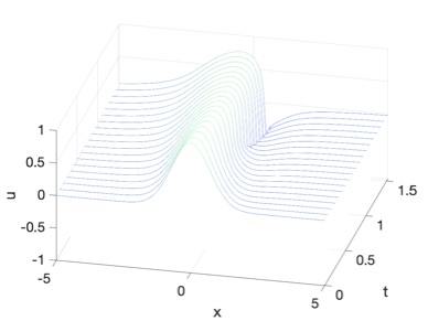
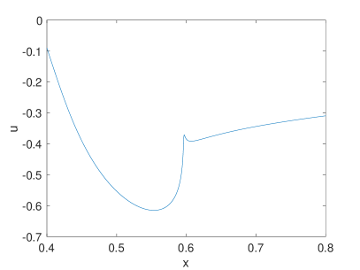
Figure 1. Solution to equation (1.1) with the $+$ sign for $\alpha=-0.5$ and the initial data $u(x,0)=\exp(-x^{2})$ in dependence of $t$ on the left, and a close-up of the solution at the final time $t=1.211$ on the right.

The computation of this cusp formation is numerically challenging. We use $N=2^{16}$ Fourier modes for $x\in 5[-\pi,\pi]$ and $N_{t}=10^{4}$ time steps for $t\in[0,1.7]$. It is known that the Fourier coefficients of an essential singularity $u\sim(x-x_{s})^{\mu}$, $\mu\in\mathbb{R}/\mathbb{Z}$ in the complex plane for $x=x_{s}$, $x_{s}\in\mathbb{C}$ are of the form

$$|\hat{u}|\sim\frac{e^{-\delta|\xi|}}{|\xi|^{1+\mu}}$$ (2.55)

for $|\xi|\gg 1$ ($\Im x_{s}=\delta>0$). Sulem, Sulem and Frisch [31] used this to characterize a singularity in solutions to hyperbolic equations via the coefficients of the discrete Fourier transform, see also [16] for a quantitative analysis. We fit the Fourier coefficients according to (2.55) during the computation. The code is stopped once $\delta$ is slightly negative in the fitting. As discussed in [16], the fitted value of $\mu$ is less reliable, but it is clear that it is positive ($\mu\sim 0.21$). It cannot be excluded that this is compatible with the value $1/3$ known from generic shocks in solutions to the Burgers’ equation, but in any case there is no $L^{\infty}$ blow-up here as expected.

If we consider the same initial data for equation (1.1) with the $-$ sign (with the same numerical parameters), the situation changes somewhat. Now the maximum gets compressed into a cusp, whereas the oscillation near the maximum which developed the cusp in Fig. 1 stays smooth. A close-up of the cusp at the time $0.8695$ can be seen on the right of the same figure. The computation is stopped at $t=0.8695$ since the fitting of the Fourier coefficients according to (2.55) produces a negative $\delta$. The fitted $\mu\sim 0.359$ is close to $1/3$.

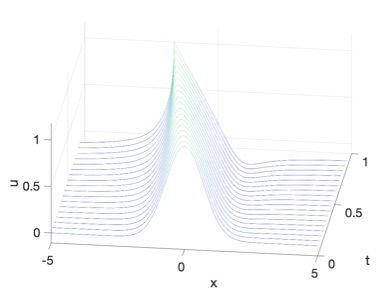
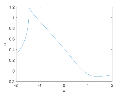
Figure 2. Solution to equation (1.1) with the $-$ sign for $\alpha=-0.5$ and the initial data $u(x,0)=\exp(-x^{2})$ in dependence of $t$ on the left, and a close-up of the solution at the final time $t=0.8695$ on the right.

If the dispersion is lowered, the situation stays qualitatively similar. For the $-$ sign in (1.1) and $\alpha=-0.8$, the code breaks for $t=0.8833$, and one gets a fitted $\mu\sim 0.357$. The solution at the final time is shown on the left of Fig. 3. The same situation for the $+$ sign in (1.1) at time $t=2.0027$ is shown on the right of the same figure. The code breaks here for the shown time with a fitted $\mu\sim 0.34$ (here we chose a slightly smaller computational domain $4[-\pi,\pi]$ in order to get somewhat higher resolution).

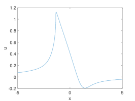
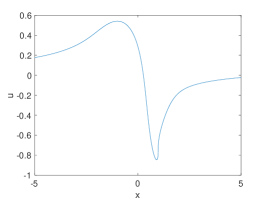
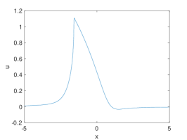
Figure 3. Solution to equation (1.1) for $\alpha=-0.8$ and the initial data $u(x,0)=\exp(-x^{2})$, with the $-$ sign at the final time $t=0.8833$ on the left, with the $+$ sign at the final time $t=2.0027$ in the middle; the solution for the equation with the $-$ sign for the same initial data and $\alpha=-0.2$ for (1.1) for $t=0.8468$ on the right.

In the case of stronger dispersion, say $\alpha=-0.2$, the situation is again similar for the Gaussian initial data and equation (1.1) with the $-$ sign. The code breaks for $t=0.8468$ with a fitted $\mu\sim 0.29$. The solution at the final time can be seen on the right of Fig. 3. However, for the equation (1.1) with the $+$ sign, we do not get a shock, but a dispersive shock wave, a zone of rapid modulated oscillations near the shock of the corresponding solution for the dispersionless equation for the same initial data. The solution for $t=1.5$ is shown in Fig. 4. This indicates that the solution stays smooth for all times in this case.

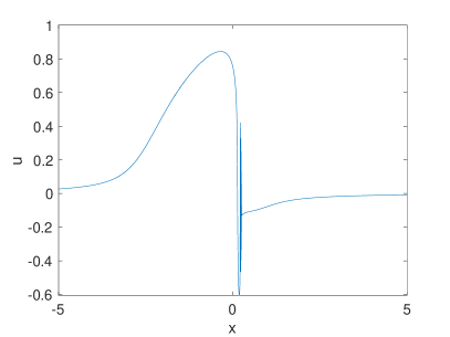
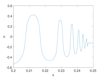
Figure 4. Solution to equation (1.1) with the $+$ sign for $\alpha=-0.2$ and the initial data $u(x,0)=\exp(-x^{2})$ for $t=1.5$ on the left, and a close-up of the solution on the right.

This of course is consistent with Proposition 1.1.

3. Variants I: shock formation for the modified Burgers-Hilbert and Whitham equations

In this section we extend the shock formation result in Theorem 2.1 to the modified Burgers-Hilbert and Whitham equations.

The modified Burgers-Hilbert equation reads as (note that the distinction between focusing and defocusing is irrelevant here):

$$u_{t}+u^{2}u_{x}-\mathcal{H}u=0,$$ (3.1)

where $\mathcal{H}=\text{p.v.}\;\frac{1}{x}$ is the Hilbert transform with Fourier symbol $-i\text{sgn}\;\xi.$ The equation (3.1) can be formally regarded as the limit case of (1.1) by letting $\alpha\rightarrow-1^{+}$.

We first state the result on the shock formation for (3.1):

Theorem 3.1.

(Rough version) There exists a wide class of functions $\phi\in H^{2}(\mathbb{R})$ with appropriate large positive amplitude $\phi$ and negative slope $\inf_{x\in\mathbb{R}}\phi^{\prime}(x)$ such that the Cauchy problem for the equation (3.1) with initial data $u(0,x)=\phi(x)$ exhibits shock formation.

(Precise version) Let $\delta$ be a sufficiently small positive number. Assume $\bar{x}_{1}$ and $\bar{x}_{2}$ are the largest and smallest numbers such that $\overline{\{x:\phi^{\prime}(x)<0\}}\subset[\bar{x}_{1},\bar{x}_{2}]$. Let $\phi\in H^{2}(\mathbb{R})$ satisfy the slope condition

$$-\inf_{x\in\mathbb{R}}\phi^{\prime}(x)>\delta^{-1}f_{1},$$

$$-\inf_{x\in\mathbb{R}}\phi^{\prime}(x)>(1-\delta)^{-2}f_{2},$$

$$-\inf_{x\in\mathbb{R}}\phi^{\prime}(x)>(1-\delta)^{-3}f_{3},$$

and the local amplitude condition

$$\phi(x)<B-(1-\delta)^{-2}f_{4},$$ (3.2)

$$\phi(x)>A+(1-\delta)^{-2}f_{4}.$$ (3.3)

for all $x\in[\bar{x}_{1},\bar{x}_{2}]$. Here the functions $(f_{1},f_{2},f_{3},f_{4})$ are homogeneous in each of its arguments of order $(1/2,0,0,0)$, and have the following explicit formulae

$$f_{1}=:f_{1}(\|\phi\|_{H^{2}},\|\phi^{\prime}\|_{L^{2}},\|\phi^{\prime\prime}\|_{L^{2}})=\big{(}C_{s}\|\phi\|_{H^{2}}+4\|\phi^{\prime}\|_{L^{2}}+64C_{m}\|\phi^{\prime\prime}\|_{L^{2}}\big{)}^{1/2},$$

$$f_{2}=:f_{2}(C_{0}^{-1}\|\phi\|_{L^{2}},C_{0}^{-1}\|\phi^{\prime}\|_{L^{2}})=6C_{0}^{-1}\|\phi\|_{L^{2}}+24C_{m}C_{0}^{-1}\|\phi^{\prime}\|_{L^{2}},$$

$$f_{3}=:f_{3}(C_{1}^{-1}\|\phi^{\prime}\|_{L^{2}},C_{1}^{-1}\|\phi^{\prime\prime}\|_{L^{2}})=8C_{1}^{-1}\|\phi^{\prime}\|_{L^{2}}+128C_{m}C_{1}^{-1}\|\phi^{\prime\prime}\|_{L^{2}},$$

$$f_{4} =:f_{4}\big{(}\|\phi\|_{L^{2}}\big{(}-\inf_{x\in\mathbb{R}}\phi^{\prime}(x)\big{)}^{-1},\|\phi^{\prime}\|_{L^{2}}\big{(}-\inf_{x\in\mathbb{R}}\phi^{\prime}(x)\big{)}^{-1}\big{)}$$

$$=\big{(}-\inf_{x\in\mathbb{R}}\phi^{\prime}(x)\big{)}^{-1}(3\|\phi\|_{L^{2}}+12C_{m}\|\phi^{\prime}\|_{L^{2}}),$$

where $C_{0}>0$ and $C_{1}>0$ satisfying

$$\|\phi\|_{L^{\infty}}\leq\frac{C_{0}}{2},\quad\|\phi^{\prime}\|_{L^{\infty}}\leq\frac{C_{1}}{2},$$

and $A>0$ and $B>0$ satisfying

$$A^{2}>8\delta B^{2},\quad B>A+2(1-\delta)^{-2}f_{4},$$

and $C_{s}$ and $C_{m}$ are the best embedding constants of Sobolev inequality and Morerry inequality

$$\|f\|_{L^{\infty}(\mathbb{R})}\leq C_{s}\|f\|_{H^{1}(\mathbb{R})},$$

and

$$|f|_{\dot{C}^{0,\frac{1}{2}}(\mathbb{R})}\leq C_{m}\|f_{x}\|_{L^{2}(\mathbb{R})},$$

where $|\cdot|_{\dot{C}^{0,\frac{1}{2}}(\mathbb{R})}$ the usual Hölder semi norm. Then the solution for the equation (3.1) with initial data $u(0,x)=\phi(x)$ exhibits shock formation at some time $T>0$ with

$$(2B+\delta)^{-1}\big{(}-\inf_{x\in\mathbb{R}}\phi^{\prime}(x)\big{)}^{-1}<T<(AB^{-1}-\delta)^{-1}(2A-\delta)^{-1}\big{(}-\inf_{x\in\mathbb{R}}\phi^{\prime}(x)\big{)}^{-1},$$

and at some location $x_{*}$ satisfying

$$\bar{x}_{1}-C_{0}^{2}T\leq x_{*}\leq\bar{x}_{2}+C_{0}^{2}T.$$

Moreover, we have the blow-up rate estimate

$$(2B+\delta)^{-1}(T-t)^{-1}\leq\|\partial_{x}u(\cdot,t)\|_{L^{\infty}}\leq(AB^{-1}-\delta)^{-1}(2A-\delta)^{-1}(T-t)^{-1},$$

as $t\rightarrow T^{-}$.

It is standard to show that the Cauchy problem for the equation (3.1) with the initial data $u(0,x)=\phi(x)$ is well-posed in the class $C([0,T):H^{2}(\mathbb{R}))$ for some $T>0$ which will be denoted the maximal time of existence in the following. Using the same notations $X(t,x),v_{0}(t,x),v_{1}(t,x),m(t)$ and $q(t)$ as (2.11)-(2.13), it then follows from (3.1) that (2.16) and (2.17) hold, in which $K_{0}(t,x)$ in (2.18) and $K_{1}(t,x)$ in (2.19) shall be respectively replaced by

$$K_{0}(t,x)=\int_{\mathbb{R}}\frac{\mathrm{sgn}(y)}{|y|}[u(t,X(t,x))-u(t,X(t,x)-y)]\,dy,$$ (3.4)

$$K_{1}(t,x)=\int_{\mathbb{R}}\frac{\mathrm{sgn}(y)}{|y|}[\partial_{x}u(t,X(t,x))-\partial_{x}u(t,X(t,x)-y)]\,dy.$$ (3.5)

Analogously, to prove Theorem 3.1, we need to show (2.20) via a contradiction argument by assuming (2.21) conversely. There are two main tasks in closing the proof of (2.21). The first task is to estimate the bound of $q(t)$, indeed one can check that Lemma 2.6 and Lemma 2.7 still hold. The other task is to show the following estimates on the nonlocal terms:

Lemma 3.2.

For all $t\in[0,T_{2}]$ and $x\in\mathbb{R}$, we have

$$|K_{0}(t,x)|\leq(2\|\phi\|_{L^{2}}+8C_{m}\|\phi^{\prime}\|_{L^{2}})q(t)^{-\frac{1}{3}},$$ (3.6)

and

$$|K_{1}(t,x)|\leq(4\|\phi^{\prime}\|_{L^{2}}+64C_{m}\|\phi^{\prime\prime}\|_{L^{2}})q(t)^{-2},$$ (3.7)

where $K_{0}(t,x)$ and $K_{1}(t,x)$ are defined by (3.4) and (3.5) respectively.

Proof.

Benefiting from the local amplitude condition (3.2)-(3.3), the solution $u$ can still live in $L^{2}(\mathbb{R})$. The proof of (3.6) and (3.7) is identical to that of [29].

∎

We now turn to the modified Whitham equation which reads

$$\partial_{t}u+u^{2}\partial_{x}u+\int_{\mathbb{R}}K(x-y)\partial_{y}u(y,t)\,dy=0,$$ (3.8)

where

$$K(x)=\frac{1}{\sqrt{2\pi}}\int_{\mathbb{R}}e^{\mathrm{i}x\xi}\sqrt{\frac{\tanh\xi}{\xi}}\,d\xi.$$

In order to deal with the modified Whitham equation we first collect the following property of $K(x)$ [10] (originally appeared in [5]):

Lemma 3.3.

There exist constants $L_{0},L_{\infty}>0$ such that

$$K(x)\leq\frac{L_{0}}{\sqrt{|x|}}\quad\mathrm{and}\quad|K^{\prime}(x)|\leq\frac{L_{0}}{\sqrt{|x|^{3}}},\quad\mathrm{for}\ 0<|x|\leq 1,$$

and

$$\int_{1}^{\infty}|K^{\prime}(x)|\,dx\leq L_{\infty}.$$

We now can state the result on the shock formation of (3.8):

Theorem 3.4.

(Rough version) There exists a wide class of functions $\phi\in H^{3}(\mathbb{R})$ with appropriate large positive amplitude $\phi$ and negative slope $\inf_{x\in\mathbb{R}}\phi^{\prime}(x)$ such that the Cauchy problem for the equation (3.8) with initial data $u(0,x)=\phi(x)$ exhibits shock formation.

(Precise version) Let $\delta$ be a sufficiently small positive number. Assume $\bar{x}_{1}$ and $\bar{x}_{2}$ are the largest and smallest numbers such that $\overline{\{x:\phi^{\prime}(x)<0\}}\subset[\bar{x}_{1},\bar{x}_{2}]$. Let $\phi\in H^{3}(\mathbb{R})$ satisfy the slope condition

$$-\inf_{x\in\mathbb{R}}\phi^{\prime}(x)>\delta^{-1}f_{1},$$

$$-\inf_{x\in\mathbb{R}}\phi^{\prime}(x)>(1-\delta)^{-2}f_{2},$$

$$-\inf_{x\in\mathbb{R}}\phi^{\prime}(x)>(1-\delta)^{-3}f_{3},$$

and the local amplitude condition

$$\phi(x)<B-(1-\delta)^{-2}f_{4},$$

$$\phi(x)>A+(1-\delta)^{-2}f_{4}.$$

for all $x\in[\bar{x}_{1},\bar{x}_{2}]$. Here the functions $(f_{1},f_{2},f_{3},f_{4})$ are homogeneous in its argument of order $(1/2,0,0,0)$, and have the following explicit formulae

$$\quad f_{1}=:f_{1}(\|\phi\|_{H^{2}},\|\phi^{\prime\prime\prime}\|_{L^{2}},C_{1})$$

$$=\big{[}C_{s}\|\phi\|_{H^{2}}+2(3L_{0}+L_{\infty})+4L_{0}(2^{-1}AB^{-1})^{-7BA^{-2}/4}C_{1}^{-1}\|\phi^{\prime\prime\prime}\|_{L^{2}}\big{]}^{1/2},$$

$$f_{2}=:f_{2}(C_{0}^{-1}C_{1})=8(3L_{0}+L_{\infty})+16L_{0}C_{0}^{-1}C_{1},$$

$$\quad f_{3}=:f_{3}(C_{1}^{-1}\|\phi^{\prime\prime\prime}\|_{L^{2}})$$

$$=4(3L_{0}+L_{\infty})+8L_{0}(2^{-1}AB^{-1})^{-7BA^{-2}/4}C_{1}^{-1}\|\phi^{\prime\prime\prime}\|_{L^{2}},$$

$$\quad f_{4}=:f_{4}\big{(}C_{0}\big{(}-\inf_{x\in\mathbb{R}}\phi^{\prime}(x)\big{)}^{-1},C_{1}\big{(}-\inf_{x\in\mathbb{R}}\phi^{\prime}(x)\big{)}^{-1}\big{)}$$

$$=\big{(}-\inf_{x\in\mathbb{R}}\phi^{\prime}(x)\big{)}^{-1}[4(3L_{0}+L_{\infty})C_{0}+8L_{0}C_{1}],$$

where $C_{0}>0$ and $C_{1}>0$ satisfying

$$\|\phi\|_{L^{\infty}}\leq\frac{C_{0}}{2},\quad\|\phi^{\prime}\|_{L^{\infty}}\leq\frac{C_{1}}{2},$$

and $A>0$ and $B>0$ satisfying

$$A^{2}>8\delta B^{2},\quad B>A+2(1-\delta)^{-2}f_{4},$$

and $C_{s}$ and $C_{m}$ are the best constants in the Sobolev inequality and Morrey inequality

$$\|f\|_{L^{\infty}(\mathbb{R})}\leq C_{s}\|f\|_{H^{1}(\mathbb{R})},$$

and

$$|f|_{\dot{C}^{0,\frac{1}{2}}(\mathbb{R})}\leq C_{m}\|f_{x}\|_{L^{2}(\mathbb{R})},$$

where $|\cdot|_{\dot{C}^{0,\frac{1}{2}}(\mathbb{R})}$ is the usual Hölder semi norm. Then the solution of equation (3.8) with initial data $u(0,x)=\phi(x)$ exhibits shock formation at some time $T>0$ with

$$(2B+\delta)^{-1}\big{(}-\inf_{x\in\mathbb{R}}\phi^{\prime}(x)\big{)}^{-1}<T<(AB^{-1}-\delta)^{-1}(2A-\delta)^{-1}\big{(}-\inf_{x\in\mathbb{R}}\phi^{\prime}(x)\big{)}^{-1},$$

and at some location $x_{*}$ satisfying

$$\bar{x}_{1}-C_{0}^{2}T\leq x_{*}\leq\bar{x}_{2}+C_{0}^{2}T.$$

Moreover, we have the blow-up rate estimate

$$(2B+\delta)^{-1}(T-t)^{-1}\leq\|\partial_{x}u(\cdot,t)\|_{L^{\infty}}\leq(AB^{-1}-\delta)^{-1}(2A-\delta)^{-1}(T-t)^{-1},$$

as $t\rightarrow T^{-}$.

It is easy to show that the Cauchy problem for the equation (3.8) with the initial data $u(0,x)=\phi(x)$ is well-posed in the class $C([0,T):H^{3}(\mathbb{R}))$ for some $T>0$ which will now denote the maximal time of existence in what follows. Using the same notations $X(t,x),v_{0}(t,x),v_{1}(t,x),m(t)$ and $q(t)$ as (2.11)-(2.13), it then follows from (3.8) that (2.16) and (2.17) hold, in which $K_{0}(t,x)$ in (2.18) and $K_{1}(t,x)$ in (2.19) shall be respectively replaced by

$$K_{0}(t,x)=\int_{\mathbb{R}}K(y)\partial_{x}u(t,X(t,x)-y)\,dy,$$ (3.9)

$$K_{1}(t,x)=\int_{\mathbb{R}}K(y)\partial_{x}^{2}u(t,X(t,x)-y)\,dy.$$ (3.10)

Arguing as above for the equation (3.1), to complete the proof of Theorem 3.4, it suffices to show the following:

Lemma 3.5.

For all $t\in[0,T_{2}]$ and $x\in\mathbb{R}$, we have

$$|K_{0}(t,x)|\leq 2\big{[}C_{0}(3L_{0}+L_{\infty})+2L_{0}C_{1}\big{]}q(t)^{-\frac{1}{2}},$$ (3.11)

and

$$|K_{1}(t,x)|\leq\big{[}2C_{1}(3L_{0}+L_{\infty})+4L_{0}(2^{-1}AB^{-1})^{-7BA^{-2}/4}\|\phi^{\prime\prime\prime}\|_{L^{2}}\big{]}q(t)^{-2},$$ (3.12)

where $K_{0}(t,x)$ and $K_{1}(t,x)$ are defined by (3.9) and (3.10) respectively.

Proof.

The proof of (3.11) can be found in [29]. Because of the stronger nonlinear term in equation (3.8), the proof here is simpler when dealing with $\|\partial_{x}^{2}u\|_{L^{\infty}}$ to estimate $K_{1}(t,x)$ than that of [29]. We only focus on the proof of (3.12). With a parameter $\eta$ being specified later, one splits the integration into the following form:

$$K_{1}(t,x) =\int_{|y|\leq\eta}K(y)\partial_{x}^{2}u(t,X(t,x)-y)\,dy$$

$$\quad+\int_{|y|>\eta}K(y)\partial_{x}^{2}u(t,X(t,x)-y)\,dy$$

$$=\colon D_{1}+D_{2}.$$

Applying Lemma 3.3, it is straightforward to see that

$$|D_{1}|\leq 2\int_{|y|\leq\eta}\frac{L_{0}}{\sqrt{|y|}}\,dy\cdot\|\partial_{x}^{2}u\|_{L^{\infty}}\leq 4L_{0}\eta^{\frac{1}{2}}\|\partial_{x}^{2}u\|_{L^{\infty}},$$ (3.13)

We use integration by parts to find that

$$|D_{2}| \leq\big{|}K(\eta)[\partial_{x}u(t,X(t,x)-\eta)-\partial_{x}u(t,X(t,x)+\eta)]\big{|}$$ (3.14)

$$\quad+\bigg{|}\int_{\eta<|y|\leq 1}K^{\prime}(y)\partial_{x}u(t,X(t,x)-y)\,dy\bigg{|}$$

$$\quad+\bigg{|}\int_{|y|>1}K^{\prime}(y)\partial_{x}u(t,X(t,x)-y)\,dy\bigg{|}$$

$$\leq 2L_{0}\eta^{-\frac{1}{2}}\|v_{1}\|_{L^{\infty}}+4L_{0}(\eta^{-\frac{1}{2}}-1)\|v_{1}\|_{L^{\infty}}+2L_{\infty}\|v_{1}\|_{L^{\infty}}$$

$$\leq 2(3L_{0}\eta^{-\frac{1}{2}}+L_{\infty})\|v_{1}\|_{L^{\infty}}\leq 2C_{1}(3L_{0}+L_{\infty})\eta^{-\frac{1}{2}}q^{-1}(t),$$

where Lemma 3.3 was used.

Again we use $\|\partial_{x}^{3}u\|_{L^{2}}$ to control $\|\partial_{x}^{2}u\|_{L^{\infty}}$. Using the property that $K(\cdot)$ is even, manipulating as (2.47) and (2.48), one still may estimate

$$\|\partial_{x}^{3}u\|_{L^{2}}\leq(2^{-1}AB^{-1})^{-7BA^{-2}/4}\|\phi^{\prime\prime\prime}\|_{L^{2}}q(t)^{-7BA^{-2}/4}.$$ (3.15)

Substituting (3.15) into (3.13) gives

$$|D_{1}|\leq 4L_{0}C_{s}(2^{-1}AB^{-1})^{-7BA^{-2}/4}\|\phi^{\prime\prime\prime}\|_{L^{2}}\eta^{\frac{1}{2}}q(t)^{-7BA^{-2}/4}.$$ (3.16)

Minimizing (3.14) and (3.16) by taking $\eta=q(t)^{-1+7BA^{-2}/4}$, one obtains

$$|K_{1}(t,x)| \leq\big{[}2C_{1}(3L_{0}+L_{\infty})+4L_{0}(2^{-1}AB^{-1})^{-7BA^{-2}/4}\|\phi^{\prime\prime\prime}\|_{L^{2}}\big{]}$$

$$\quad\times q(t)^{7BA^{-2}/8-1/2}$$

$$\leq\big{[}2C_{1}(3L_{0}+L_{\infty})+4L_{0}(2^{-1}AB^{-1})^{-7BA^{-2}/4}\|\phi^{\prime\prime\prime}\|_{L^{2}}\big{]}q(t)^{-2}.$$

This finishes the proof of (3.12).

∎

We illustrate the shock formation in solutions of the modified Whitham equation for the example of Gaussian initial data. In this case the code is stopped for $t=0.8511$ since the Fourier coefficients are no longer exponentially decreasing. The solution at this time can be seen in Fig. 5. A fitting of the Fourier coefficients according to (2.55) yields a $\mu\sim 0.38$. Thus the shock formation appears to be as for the modified fKdV equation with negative $\alpha$.

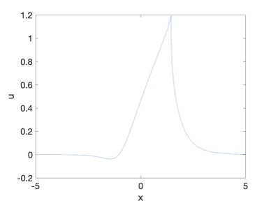
Figure 5. Solution to the modified Whitham equation for the initial data $u(x,0)=\exp(-x^{2})$ for $t=0.8511$.

4. Variants II: shock formation for the generalized fractional Korteweg-de Vries equation

The generalized fractional Korteweg-de Vries equation reads :

$$u_{t}+u^{p}u_{x}-|D|^{\alpha}\partial_{x}u=0,\;p=3,4,...$$ (4.1)

The result on the shock formation of (4.1) can be stated as follows:

Theorem 4.1.

(Rough version) Let $p>1$ and $\alpha\in(-1,0)$. There exists a wide class of functions $\phi\in H^{3}(\mathbb{R})$ with appropriate large positive amplitude $\phi$ and negative slope $\inf_{x\in\mathbb{R}}\phi^{\prime}(x)$ such that the Cauchy problem for equation (4.1) with initial data $u(0,x)=\phi(x)$ exhibits shock formation.

(Precise version) Let $p>1$ and $\alpha\in(-1,0)$, and $\delta$ be a sufficiently small positive number. Assume $\bar{x}_{1}$ and $\bar{x}_{2}$ are the largest and smallest numbers such that $\overline{\{x:\phi^{\prime}(x)<0\}}\subset[\bar{x}_{1},\bar{x}_{2}]$. Let $\phi\in H^{3}(\mathbb{R})$ satisfy the slope condition

$$-\inf_{x\in\mathbb{R}}\phi^{\prime}(x)>\delta^{-1}f_{1},$$

$$-\inf_{x\in\mathbb{R}}\phi^{\prime}(x)>(1-\delta)^{-2}f_{2},$$

$$-\inf_{x\in\mathbb{R}}\phi^{\prime}(x)>(1-\delta)^{-3}f_{3},$$

and the local amplitude condition

$$\phi(x)<B-(1-\delta)^{-2}f_{4},$$

$$\phi(x)>A+(1-\delta)^{-2}f_{4},$$

for all $x\in[\bar{x}_{1},\bar{x}_{2}]$. Here the functions $(f_{1},f_{2},f_{3},f_{4})$ are homogeneous in each argument of order $(1/2,0,0,0)$, and have the following explicit formulae

$$f_{1} =:f_{1}(\|\phi\|_{H^{2}},C_{1},\|\phi^{\prime\prime\prime}\|_{L^{2}})=\big{[}C_{s}\|\phi\|_{H^{2}}+4C_{1}(1+\alpha)^{-1}$$

$$\quad+2C_{s}(-\alpha)^{-1}(2^{-1}A^{p-1}B^{1-p})^{-7B^{p-1}/(2pA^{2p-2})}\|\phi^{\prime\prime\prime}\|_{L^{2}}\big{]}^{1/2},$$

$$f_{2}=:f_{2}(C_{0}^{-1}C_{1})=8(-\alpha(1+\alpha))^{-1}+4\alpha^{-2}C_{0}^{-1}C_{1},$$

$$\quad f_{3}=:f_{3}(C_{1}^{-1}\|\phi^{\prime\prime\prime}\|_{L^{2}})$$

$$=8(1+\alpha)^{-1}+4C_{s}(-\alpha)^{-1}(2^{-1}A^{p-1}B^{1-p})^{-7B^{p-1}/(2pA^{2p-2})}C_{1}^{-1}\|\phi^{\prime\prime\prime}\|_{L^{2}},$$

$$\quad f_{4}=:f_{4}\big{(}C_{0}\big{(}-\inf_{x\in\mathbb{R}}\phi^{\prime}(x)\big{)}^{-1},C_{1}\big{(}-\inf_{x\in\mathbb{R}}\phi^{\prime}(x)\big{)}^{-1}\big{)}$$

$$=\big{(}-\inf_{x\in\mathbb{R}}\phi^{\prime}(x)\big{)}^{-1}\big{[}4C_{0}\big{(}-\alpha(1+\alpha)\big{)}^{-1}+2C_{1}\alpha^{-2}\big{]},$$

where $C_{0}>0$ and $C_{1}>0$ satisfying

$$\|\phi\|_{L^{\infty}}\leq\frac{C_{0}}{2},\quad\|\phi^{\prime}\|_{L^{\infty}}\leq\frac{C_{1}}{2},$$

and $A>0$ and $B>0$ satisfying

$$A^{2p-2}>8\delta B^{2p-2},\quad 4pA^{2p-2}>7B^{p-1},\quad B>A+2(1-\delta)^{-2}f_{4},$$ (4.2)

and $C_{s}$ is the best constant of the Sobolev inequality

$$\|f\|_{L^{\infty}(\mathbb{R})}\leq C_{s}\|f\|_{H^{1}(\mathbb{R})}.$$

Then the solution for the equation (4.1) with initial data $u(0,x)=\phi(x)$ exhibits shock formation at some time $T>0$ satisfying

$$(pB^{p-1}+\delta)^{-1}\big{(}-\inf_{x\in\mathbb{R}}\phi^{\prime}(x)\big{)}^{-1}<T$$

$$<(A^{p-1}B^{1-p}-\delta)^{-1}(pA^{p-1}-\delta)^{-1}\big{(}-\inf_{x\in\mathbb{R}}\phi^{\prime}(x)\big{)}^{-1},$$

and at some location $x_{*}$ satisfying

$$\bar{x}_{1}-C_{0}^{p}T\leq x_{*}\leq\bar{x}_{2}+C_{0}^{p}T.$$ (4.3)

Moreover, we have the blow-up rate estimate

$$(pB^{p-1}+\delta)^{-1}(T-t)^{-1}\leq\|\partial_{x}u(\cdot,t)\|_{L^{\infty}}$$

$$\leq(A^{p-1}B^{1-p}-\delta)^{-1}(pA^{p-1}-\delta)^{-1}(T-t)^{-1},$$

as $t\rightarrow T^{-}$.

It is standard to show that the Cauchy problem for the equation (4.1) with the initial data $u(0,x)=\phi(x)$ is well-posed in the class $C([0,T):H^{3}(\mathbb{R}))$ for some $T>0$ which will now denote the maximal time of existence. Using the same notations $X(t,x),v_{0}(t,x),v_{1}(t,x),m(t)$ and $q(t)$ as (2.11)-(2.13), it then follows from (4.1) that (2.16) and (2.17) hold, in which $K_{0}(t,x)$ and $K_{1}(t,x)$ are the same as in (2.18) and (2.19).

Analogously, to prove Theorem 4.1, we need to show (2.20) via a contradiction argument by assuming (2.21) conversely. We need to carrry two main tasks to close the proof of (2.21).

The first task is to estimate the bound of $q(t)$. Let $t\in[0,T_{1}]$ and $x\in[\bar{x}_{1},\bar{x}_{2}]$, and a priori assume

$$A\leq v_{0}(t,x)\leq B,$$

in which $A$ and $B$ are given in Theorem 4.1 satisfying (4.2). We now define

$$\Sigma_{\delta}(t)=\{x\in[\bar{x}_{1},\bar{x}_{2}]:\ v_{1}(t,x)\leq(A^{p-1}B^{1-p}-\delta)m(t)\},$$

and

$$v_{1}(t,x)=:m(0)r^{-1}(t,x).$$

With slight modifications, one can follow the proof of Lemma 2.6-Lemma 2.7 to show the following:

Lemma 4.2.

We have $\Sigma_{\delta}(t_{2})\subset\Sigma_{\delta}(t_{1})$ whenever $0\leq t_{1}\leq t_{2}\leq T_{1}$.

Lemma 4.3.

$q(t)$ is decreasing and satisfies

$$0<q(t)\leq 1,\quad\text{for}\ t\in[0,T_{1}].$$

We also have the integral estimates

$$\int_{0}^{t}q^{-s}(\tau)\,d\tau \leq(1-s)^{-1}m^{-1}(0)(pA^{p-1}-\delta)^{-1}(A^{p-1}B^{1-p}-\delta)^{-s}$$

$$\quad\times\big{[}q^{1-s}(t)-(A^{p-1}B^{1-p}-\delta)^{s-1}\big{]},\quad\text{for}\ t\in[0,T_{1}].$$

where $s>0,s\neq 1$, and

$$\int_{0}^{t}q^{-1}(\tau)\,d\tau \leq m^{-1}(0)(pA^{p-1}-\delta)^{-1}(A^{p-1}B^{1-p}-\delta)^{-1}$$

$$\quad\times\big{[}\log(A^{p-1}B^{1-p}-\delta)+\log q(t)\big{]},\quad\text{for}\ t\in[0,T_{1}].$$

The other task is to estimate the nonlocal terms.

Lemma 4.4.

For all $t\in[0,T_{2}]$ and $x\in\mathbb{R}$, we have

$$|K_{0}(t,x)|\leq\big{[}4C_{0}(1+\alpha)^{-1}+2C_{1}(-\alpha)^{-1}\big{]}q(t)^{-(1+\alpha)},$$

and

$$|K_{1}(t,x)| \leq\big{[}4C_{1}(1+\alpha)^{-1}+2C_{s}(-\alpha)^{-1}$$

$$\quad\times(2^{-1}A^{p-1}B^{1-p})^{-7B^{p-1}/(2pA^{2p-2})}\|\phi^{\prime\prime\prime}\|_{L^{2}}\big{]}q^{-2}(t),$$

Proof.

Compared with the proof of Lemma 4.4, the only difference is to apply Lemma 4.3 to replace Lemma 2.7 to estimate $\|\partial_{x}^{3}u\|_{L^{2}}$ by using (2.47)

$$\|\partial_{x}^{3}u\|_{L^{2}} \leq\|\phi^{\prime\prime\prime}\|_{L^{2}}(A^{p-1}B^{1-p}-\delta)^{-\frac{7}{2(pA^{p-1}-\delta)(A^{p-1}B^{1-p}-\delta)}}$$

$$\quad\times q(t)^{-\frac{7}{2(pA^{p-1}-\delta)(A^{p-1}B^{1-p}-\delta)}}$$

$$\leq(2^{-1}A^{p-1}B^{1-p})^{-7B^{p-1}/(2pA^{2p-2})}\|\phi^{\prime\prime\prime}\|_{L^{2}}q(t)^{-7B^{p-1}/(2pA^{2p-2})}.$$

∎

We finally note that one can similarly extend the result in Theorem 4.1 to the generalized Burgers-Hilbert and Whitham equations (the cubic nonlinearity $u^{2}u_{x}$ being replaced by the generalized nonlinearity $u^{p}u_{x}$ $(p>1)$ in (3.1) and (3.8)).

5. The case $\alpha>0$

As aforementioned, most assertions in this Section are conjectures that will be motivated by numerical simulations.

5.1. Solitary waves

We first state and recall some theoretical results, starting by the solitary wave solutions, that is solutions of the form

$$u_{c}(x,t)=Q_{c}(x-ct),$$

where $Q_{c}\in H^{\alpha/2}(\mathbb{R}).$ They should satisfy the equation

$$D^{\alpha}Q_{c}+cQ_{c}\mp\frac{1}{3}Q_{c}^{3}=0.$$ (5.1)

The first one is classical and concerns the non-existence of solitary waves.

Proposition 5.1.

There exists no nontrivial solitary waves of (1.1):

1. In the defocusing case for all $\alpha>0$;

2. In the focusing case when $0<\alpha\leq 1/2$ (energy super critical).

Proof.

The proof is similar to that of the quadratic case (see [20]). By (5.1), we have the energy identity

$$\int_{\mathbb{R}}|D^{\alpha/2}Q_{c}|^{2}\,dx+c\int_{\mathbb{R}}Q_{c}^{2}\,dx\mp\frac{1}{3}\int_{\mathbb{R}}Q_{c}^{4}\,dx=0,$$

and the Pohozaev identity

$$\frac{\alpha-1}{2}\int_{\mathbb{R}}|D^{\alpha/2}Q_{c}|^{2}\,dx-\frac{c}{2}\int_{\mathbb{R}}Q_{c}^{2}\,dx\pm\frac{1}{12}\int_{\mathbb{R}}Q_{c}^{4}\,dx=0,$$

which in turn is a consequence of the identity (see for instance Lemma 3 in [14])

$$\int_{\mathbb{R}}(D^{\alpha}\phi)x\phi^{\prime}\,dx=\frac{\alpha-1}{2}\int_{\mathbb{R}}|D^{\alpha/2}\phi|^{2}\,dx,$$

imply in the focusing case

$$(1-2\alpha)\int_{\mathbb{R}}|D^{\alpha/2}Q_{c}|^{2}\,dx+c\int_{\mathbb{R}}Q_{c}^{2}\,dx=0$$

proving that no finite energy solitary waves exist in the energy supercritical case $\alpha>1/2$ when $c\leq 0$.

The same conclusion holds for any $\alpha>0$ in the defocusing case just by the energy identity.

∎

The existence of non trivial solutions for (5.1) in the admissible range is standard and we refer for instance to [8] from which we extract the

Proposition 5.2.

Let $1/2<\alpha<2$.

(i) (Existence) There exists a solution $Q\in H^{\alpha/2}(\mathbb{R})$ of (5.1) such that $Q(|x|)>0$ is even, positive and strictly decreasing in $|x|.$

(ii) (Symmetry and monotonicity) If $Q\in H^{\alpha/2}(\mathbb{R})$ with $Q\geq 0$ and $Q\not\equiv 0,$ then there exists $x_{0}\in\mathbb{R}$ such that $Q(\cdot-x_{0})$ is even, positive and strictly decreasing in $|x-x_{0}|.$

(iii) (Regularity and decay) If $Q\in H^{\alpha/2}(\mathbb{R})$ solves (5.1), then $Q\in H^{\alpha+1}(\mathbb{R}).$ Moreover we have the decay estimate

$$|Q(x)|+|xQ^{\prime}(x)|\leq\frac{C}{1+|x|^{\alpha+1}},$$

for all $x\in\mathbb{R}$ and some constant $C>0.$

Remark 5.3.

In fact $Q$ can be obtained as a minimizer of the Weinstein functional

$$J^{\alpha}(u)=\left(\int_{\mathbb{R}}|u|^{4}\,dx\right)^{-1}\left(\int_{\mathbb{R}}|D|^{\alpha/2}u|^{2}\,dx\right)^{1/\alpha}\left(\int_{\mathbb{R}}u^{2}\,dx\right)^{2-\frac{1}{\alpha}},$$

or optimizers of the Gagliardo-Nirenberg inequality

$$\int_{\mathbb{R}}|u|^{4}\,dx\leq C_{\alpha}\left(\int_{\mathbb{R}}|D|^{\alpha/2}u|^{2}\,dx\right)^{1/\alpha}\left(\int_{\mathbb{R}}u^{2}\,dx\right)^{2-\frac{1}{\alpha}},.$$

Actually, following [8], for $\alpha>1/2,$ a ground state solution of

$$D^{\alpha}Q+Q-Q^{3}/3=0$$ (5.2)

is a positive and even solution that minimizes the Weinstein functional on $H^{\alpha/2}(\mathbb{R})\setminus\{0\}.$

Concerning stability, one can in a straightforward way extend the results of [20] that concerned the (quadratic) fKdV equation to the focusing modified fKdV equation to prove that the ground state is (conditionally) stable in the $L^{2}$ subcritical case $\alpha>1$. We refer to [26] for a complete analysis of stability issues for the focusing modified fKdV equation (and of fKdV with higher nonlinearities) in the $L^{2}$ subcritical regime.

Note that

$$Q_{c}(x)=\sqrt{c}Q(c^{1/\alpha}x),$$

where we have put $Q_{1}=Q$, so that

$$\|Q_{c}\|_{L^{2}}^{2}=c^{\frac{\alpha-1}{\alpha}}\|Q\|_{L^{2}}^{2},$$

proving that the solitary waves may have arbitrary small $L^{2}$ norm by taking arbitrary large velocities when $1/2<\alpha<1$ (resp. arbitrary small velocities when $\alpha>1$). This excludes scattering of small solutions in the $L^{2}$ norm.

The case $\alpha=1$ (modified Benjamin-Ono) is $L^{2}$ critical and the solitary waves have constant $L^{2}$ norm.

Similarly,

$$\|D^{\alpha/2}Q_{c}\|_{L^{2}}^{2}=c^{\frac{3\alpha-2}{2\alpha}}\|D^{\alpha/2}Q\|^{2}_{L^{2}}$$

proving for instance that no scattering in the energy norm is possible when $1/2<\alpha<1$.

We show some ground states of the equation (1.1) with the $+$ sign for $c=1$ and various values of $\alpha$ in Fig. 6. The ground states get more and more peaked the smaller the dispersion is. Compared to the ground states for the fKdV equation in [18] their maximum is smaller here because of the higher nonlinearity.

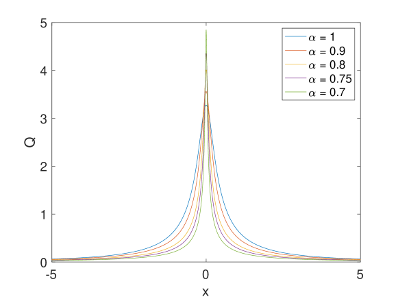
Figure 6. Ground states of the equation (1.1) with the $+$ sign for $c=1$ and various values of $\alpha$.

5.2. The Cauchy problem: generalities

It is straightforward to prove that the modified fKdV equation is locally well posed in $H^{s}(\mathbb{R}),s>3/2$ when $\alpha\geq-1.$ On the other hand the modified Burgers equation is ill-posed in $H^{3/2}(\mathbb{R})$ as can be checked by extending the proof in [19] for the usual Burgers equation.

Adding a dispersive perturbation ($\alpha>0$) has the effect to enlarge the space of resolution for the local Cauchy problem. Actually it was proven in [20] that the Cauchy problem for the fKdV equation is locally well-posed in $H^{s}(\mathbb{R}),s>\frac{3}{2}-\frac{3\alpha}{8}.$ This was improved in [23] to $s>\frac{3}{2}-\frac{5\alpha}{4}$ leading to the global well-posedness of the Cauchy problem in the energy space when $\alpha>6/7.$ The expected global well-posedness for the whole range $1/2<\alpha<1$ is still open.

A similar enlargement of the space of the resolution for the local Cauchy problem is expected for the modified fKdV equation but this is outside the scope of the present paper that is focused on global issues. We just recall that the Cauchy problem for the modified Benjamin-Ono ($\alpha=1$), in both the focusing and defocusing case, was proven to be locally well-posed in $H^{s}(\mathbb{R}),s\geq 1/2$ by Kenig and Takaoka [15] extending a previous work of Molinet and Ribaud [24] who proved the result for $s>1/2.$

5.3. The Cauchy problem: focusing case

For the focusing modified Benjamin-Ono equation ($\alpha=1$), Martel and Pilod [21] proved the finite time blow-up by constructing a minimal mass blow-up solution.

For the other values of $\alpha$ we a priori formulate the following conjectures which will be reinforced by the numerical simulations below:

(i) Finite time blow-up in the case $1/2<\alpha<1$ similar to the gKdV equation

$$u_{t}+u^{p}u_{x}+u_{xxx}=0,$$

when $p>4.$

(ii) Finite time blow-up in the energy supercritical case $0<\alpha<1/2.$

(iii) Global well-posedness and soliton resolution when $\alpha>1.$

Remark 5.4.

It is well known that the focusing modified KdV equation possesses special solutions that are periodic in t and localized in x, the so-called breather solution (see for instance [1] and the references therein). Establishing the existence of such solutions for the focusing modified mKdV when $\alpha>1/2$ is an interesting open question.

5.4. The Cauchy problem: defocusing case

In the energy subcritical case $\alpha>1/2$, one obtains classically by a compactness method the global existence of weak solutions:

Proposition 5.5.

Let $\alpha>1/2$ and $u_{0}\in H^{\alpha/2}(\mathbb{R}).$ Then there exists a solution $u\in L^{\infty}(\mathbb{R}:H^{\alpha/2}(\mathbb{R}))$ of (1.1) with initial data $u_{0}.$

We recall that for the modified defocusing Benjamin-Ono equation ($\alpha=1$) Kenig and Takaoka [15] proved the global well-posedness in $H^{s}(\mathbb{R}),s\geq 1/2$.

One might a priori conjecture that global well-posedness holds for $\alpha>1/2$ but the case $0<\alpha\leq 1/2$ is unclear.

We now present numerical simulations that support the previous conjectures.

Equation (1.1) is invariant under the rescaling

$$y=\frac{x}{L},\quad\frac{d\tau}{dt}=\frac{1}{L^{1+\alpha}},\quad U=L^{\alpha/2}u,$$ (5.3)

i.e., if $u(x,t)$ is a solution to equation (1.1), so is $U(y,\tau)$ for constant $L$. If in (5.3) one lets $L$ depend on $\tau$, one speaks of a dynamic rescaling, and (1.1) takes the form

$$U_{\tau}-\partial_{\tau}(\ln L)(yU_{y}+\alpha U/2)\pm U^{2}U_{y}-|D_{y}|^{\alpha}U_{y}=0.$$ (5.4)

The mass $m[u]$ (the square of the $L^{2}$ norm) and the energy $H[u]$ have the following scaling behavior under (5.3),

$$m[U]=L^{1-\alpha}m[u],\quad H[U]=L^{1-2\alpha}H[u].$$ (5.5)

This means, as was previously noticed, the equation (1.1) is $L^{2}$ critical for $\alpha=1$, the modified Benjamin-Ono equation, and energy critical for $\alpha=1/2$. Thus a self-similar blow-up is expected in the focusing case for $0<\alpha\leq 1$, in the rescaling (5.3) such that $\tau\to\infty$ and $L(\tau)\to 0$ in this case. In this limit, one gets the blow-up profile $U^{\infty}$ from (5.4),

$$a^{\infty}(yU_{y}^{\infty}+\alpha U^{\infty}/2)+(U^{\infty})^{2}U_{y}^{\infty}-|D_{y}|^{\alpha}U_{y}^{\infty}=0,$$ (5.6)

where $a=-(\ln L)_{\tau}$ and $\lim_{\tau\to\infty}a=a^{\infty}$. In the $L^{2}$ critical case one expects $a^{\infty}=0$ in which case the blow-up profile will be just the solitary wave of the modified Benjamin-Ono equation. In the general case, the blow-up profile depends on $a^{\infty}$, and it is not known whether there are localized solutions to (5.6).

In [12], we have studied blow-up in solutions to generalized KdV equations, and it was shown that it is numerically problematic to solve the rescaled equation (5.4). Instead we solved the generalized KdV equation numerically, and fitted certain norms as the $\|u\|_{L^{\infty}}$ and $\|u_{x}\|_{L^{2}}$ to certain blow-up models. In the $L^{2}$ critical case one expects $L\propto 1/\tau$, and thus

$$\|u\|_{L^{\infty}}\propto(t^{*}-t)^{-1/2},\quad\|u_{x}\|_{L^{2}}^{2}\propto(t^{*}-t)^{-(1+1/\alpha)}.$$ (5.7)

In the $L^{2}$ supercritical one expects $L\propto\exp(-\kappa\tau)$ with $\kappa>0$. In this case one has

$$\|u\|_{L^{\infty}}\propto(t^{*}-t)^{-\alpha/(1+\alpha)/2},\quad\|u_{x}\|_{L^{2}}^{2}\propto(t^{*}-t)^{-1}.$$ (5.8)

In the case of a blow-up, these norms will be fitted to the above models to validate the conjectured blow-up scenario.

5.5. Numerical study of the focusing case

We first consider the focusing $L^{2}$ subcritical case for $\alpha=1.5$ with $N=2^{12}$ Fourier modes for $x\in 10[-\pi,\pi]$ and $N_{t}=10^{4}$ time steps for $t\in[0,1]$. For small enough initial data, there is just dispersion of the data as can be seen for the initial data $u(x,0)=\exp(-x^{2})$ on the left of Fig. 7 on the left. Dispersive radiation is emitted to the left, no stable structure seems to appear. This is also confirmed by the $L^{\infty}$ norm of the solution in the same figure on the right. It appears to be monotonically decreasing.

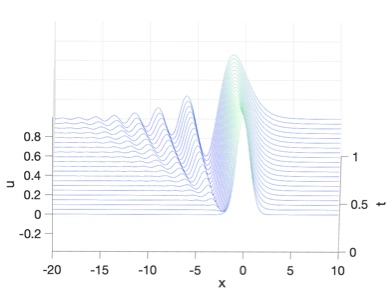
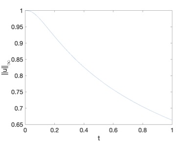
Figure 7. Solution to equation (1.1) with the $+$ sign for $\alpha=1.5$ and the initial data $u(x,0)=\exp(-x^{2})$ on the left, and the $L^{\infty}$ norm of the solution on the right.

We are here in a scattering scenario which suggests that the initial data $u(x,0)=\exp(-x^{2})$ leads to a solution without solitary waves.

The situation changes if initial data of larger norm are considered. In Fig. 8 we show the solution in the same setting as in Fig. 7, but this time for the initial data $u(x,0)=5\exp(-x^{2})$. In addition to the dispersive radiation emitted towards $-\infty$, there is now a solitary wave traveling to the right.

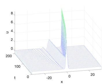
Figure 8. Solution to equation (1.1) with the $+$ sign for $\alpha=1.5$ and the initial data $u(x,0)=5\exp(-x^{2})$.

This is confirmed by the $L^{\infty}$ norm of the solution on the left of Fig. 9. To make this even more explicit, we show on the right of the same figure the solution of Fig. 8 at the final time $t=1$ together with the solitary wave fitted according to (5.1) in green. It can be seen that the solitary wave is already fully developed, possibly the smaller hump to the left of the large solitary wave will become a ground state of smaller velocity. This suggests that the soliton resolution conjecture also applies to this equation.

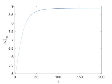
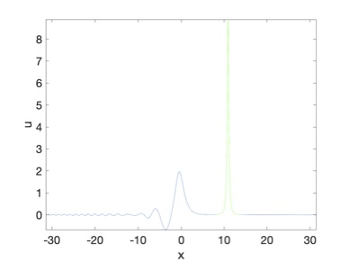
Figure 9. $L^{\infty}$ norm of the solution to equation (1.1) with the $+$ sign for $\alpha=1.5$ and the initial data $u(x,0)=5\exp(-x^{2})$ on the left, and the solution for $t=1$ with a fitted solitary wave on the right in green.

Next we consider the $L^{2}$ critical case $\alpha=1$, i.e., the modified Benjamin-Ono equation. For the initial data $u(x,0)=5\exp(-x^{2})$, we use $N=2^{14}$ Fourier modes for $x\in 5[-\pi,\pi]$ and $N_{t}=10^{4}$ time steps for $t\in[0,0.081]$. The code breaks shortly after the final time since relative energy conservation is no longer assured to the order of $10^{-3}$. The solution for various values of $t$ can be seen in Fig. 10. A solitary wave detaches from the initial hump and eventually appears to blow up.

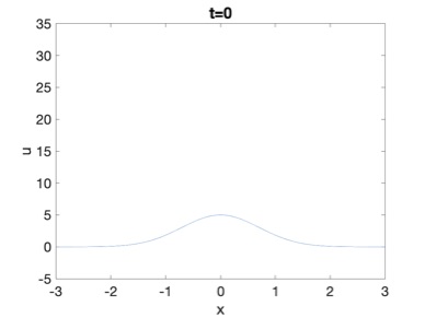
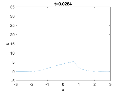
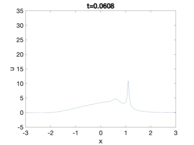
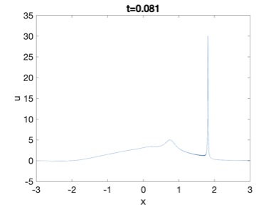
Figure 10. Solution to equation (1.1) with the $+$ sign for $\alpha=1$ for the initial data $u(x,0)=5\exp(-x^{2})$ at various times.

An $L^{\infty}$ blow-up is also confirmed by the $L^{\infty}$ norm and the $L^{2}$ norm of the gradient as shown in Fig. 11.

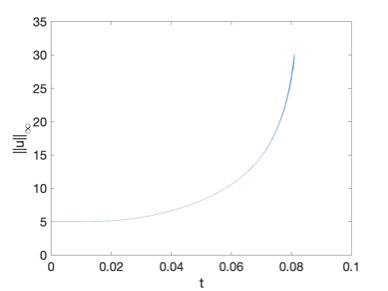
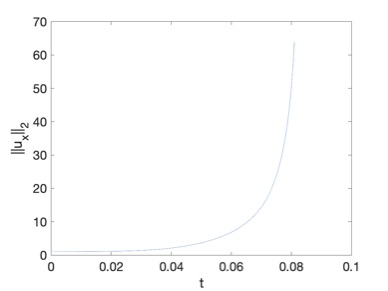
Figure 11. $L^{\infty}$ norm on the left and $\|u_{x}\|_{L^{2}}$ (normalized to 1 for $t=0$) on the right for the solution to equation (1.1) with the $+$ sign for $\alpha=1$ for the initial data $u(x,0)=5\exp(-x^{2})$.

If we fit the norms in Fig. 11 for the last 500 time steps according to

$$\ln\|u\|_{L^{\infty}}\sim a\ln(t^{*}-t)+b$$ (5.9)

in [18], then we get a minimum residual for the values $a=-0.54$, $b=0.49$, and $t^{*}=0.0854$. Similarly we get for $\|u_{x}\|_{L^{2}}$ the fitted values $a=-1.04$, $b=-1.62$ and $t^{*}=0.085$. The good agreement of the blow-up times $t^{*}$ is an indicator of the quality of these results which do not change much if a slightly smaller or larger number of points are taken into account for the fitting. The results for the scaling exponents are in accordance with the expectation for the critical case in (5.7). In Fig. 12 we show the solution at the last recorded time together with a rescaled soliton (according to (5.3), the ratio of the maximum of $u$ and $Q$ respectively determines the factor $L^{\alpha/2}$). It can be seen that the blow-up profile is given by the ground state though the blow-up has not yet been reached. Note that we obtain the same behavior for the $-$ sign in equation (6.1).

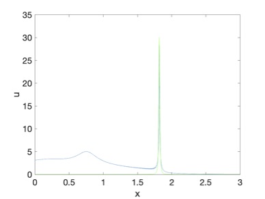
Figure 12. Solution to equation (1.1) with the $+$ sign for $\alpha=1$ for the initial data $u(x,0)=5\exp(-x^{2})$ for $t=0.081$ and a rescaled soliton according to (5.3) in green.

As an example for the $L^{2}$ supercritical (but energy subcritical) case, we consider $\alpha=0.8$, the initial data $u(x,0)=3\exp(-x^{2})$ and $t\in[0,0.22]$. We use $N=2^{14}$ Fourier modes for $x\in 2[-\pi,\pi]$ and $N_{t}=10^{4}$ time steps. The code is stopped for $t=0.2123$ since the relative energy conservation drops below $10^{-3}$ shortly afterwards. The solution at this time can be seen in Fig. 13. The profile of the blow-up is clearly different from the $L^{2}$ critical one in Fig. 12 .

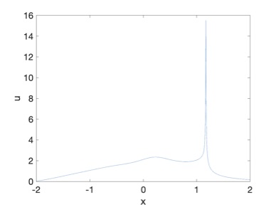
Figure 13. Solution to equation (1.1) with the $+$ sign for $\alpha=0.8$ for the initial data $u(x,0)=3\exp(-x^{2})$ for $t=0.2123$.

If we fit the $L^{\infty}$ norm of the solution for the last 100 recorded time steps (the results are similar for a slightly larger number of steps) according to (5.9), we find $a=-0.27$, $b=1.01$, and $t^{*}=0.2140$. An analogous fitting for $\|u_{x}\|_{L^{2}}$ yields $a=-0.62$, $b=0.14$, and $t^{*}=0.2140$. Note the excellent agreement for the blow-up time. From (5.8) one would expect in the former case for $a$ a value of $-0.222$, and in the latter $-0.5$. This means that the agreement with expectation is better for the $L^{\infty}$ norm, and that we are not close enough to the blow-up (on the rescaled time scales since the blow-up is expected to be exponential in $\tau$) for $\|u_{x}\|_{L^{2}}$.

In the energy critical case $\alpha=0.5$ and the energy supercritical case $\alpha=0.4$, we consider the initial data $u(x,0)=2\exp(-x^{2})$ with the same numerical parameters. The codes break for $t=0.3281$ and $t=0.2674$ respectively in the sense that the relative energy conservation drops below $10^{-3}$.

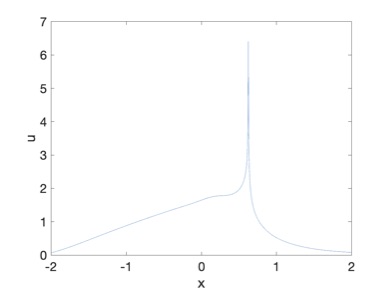
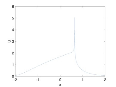
Figure 14. Solutions to equation (1.1) with the $+$ sign for the initial data $u(x,0)=2\exp(-x^{2})$ at the times where the code breaks, on the left for $\alpha=0.5$, on the right for $\alpha=0.4$.

Fitting the norms for the last 100 recorded time steps to (5.9), we get in the case $\alpha=0.5$ for the $L^{\infty}$ norm $a=-0.168$ (expected value $-1/6$) and for the $\|u_{x}\|_{L^{2}},$ $a=-0.47$ (expected value $-1/2$) with blow-up times of $0.3298$ and $0.3296$ respectively. Thus an excellent agreement between the blow-up times and the expectation for the scalings is observed. For $\alpha=0.4$, we get for the $L^{\infty}$ norm $a=-0.14$ (expected value $-0.1429$), and $a=-0.66$ (expected value $-0.5$) for $\|u_{x}\|_{L^{2}}$. In both cases the blow-up time is determined to be $0.2685$.

The above results can be summarized in the following

Conjecture 5.6.

Consider smooth initial data $u_{0}\in L^{2}(\mathbb{R})$ with a single hump for the focusing equation (1.1). Then for

• $\alpha>1$: solutions to the focusing modified fKdV equations with the initial data $u_{0}$ stay smooth for all $t$. For large $t$ they decompose asymptotically into solitary waves and radiation.

• $0<\alpha\leq 1$: solutions to the focusing modified fKdV equations with initial data $u_{0}$ of sufficiently small, but non-zero mass stay smooth for all $t$.

• $\alpha=1$: solutions to the focusing modified fKdV equations with the initial data $u_{0}$ with negative energy and mass larger than the solitary wave mass blow up at finite time $t^{*}$. The type of the blow-up for $t\nearrow t^{*}$ is characterized by

  $$u(x,t)\sim\frac{1}{\sqrt{L(t)}}Q\left(\frac{x-x_{m}}{L(t)}\right),\quad L=c_{0}(t^{*}-t),$$

  where $c_{0}$ is a constant, and where $Q$ is the solitary wave solution (5.1) for $c=1$.

• $0<\alpha<1$: solutions to the focusing modified fKdV equations with the initial data $u_{0}$ and sufficiently large $L^{2}$ norm blow up at finite time $t^{*}$ and finite $x=x^{*}$. The nature of blow-up is self similar as given by (5.3), but the blow-up profile appears to be given by (5.6) with non-vanishing $a^{\infty}$.

Remark 5.7.

The numerical study of the appearance of singularities in solutions to PDEs pushes all numerical methods to the limits, and the results always have to be taken with a grain of salt. The results we present in this paper are always stable with respect to moderate changes of the numerical resolution. In addition we fit in the case of shocks the Fourier coefficients and in the case of $L^{\infty}$ blow-ups various norms. Nonetheless all numerical results are with finite precision, and the analytical phenomena to be studied can always be inaccessible within this precision.

5.6. Numerical study of the defocusing case

The same initial data as in Fig. 8 for the defocusing equation (1.1) lead only to dispersion as can be seen in Fig. 15. This is once more indication for the absence of stable structures in the defocusing case.

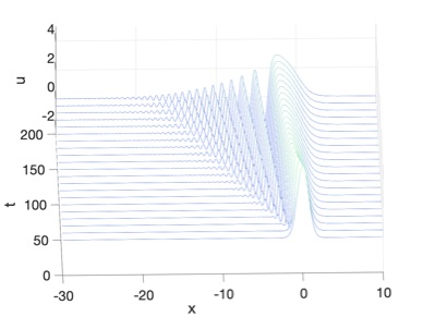
Figure 15. Solution to equation (1.1) with the $-$ sign for $\alpha=1.5$ and the initial data $u(x,0)=5\exp(-x^{2})$.

In the energy critical case $\alpha=0.5$, solutions to the defocusing equation (1.1) still appear to be dispersed. We use $N=2^{14}$ Fourier modes for $x\in 5[-\pi,\pi]$ and $N_{t}=10^{4}$ time steps for $t\in[0,0.05]$. As can be seen on the left of Fig. 16, there appears to be a strong gradient to the right of the initial hump, but the dispersion is still sufficient to create a DSW as is even more clear from the close-up of this zone on the right of the same figure.

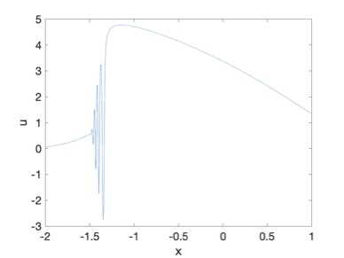
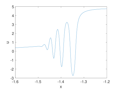
Figure 16. Solution to equation (1.1) with the $-$ sign for $\alpha=0.5$ for the initial data $u(x,0)=5\exp(-x^{2})$ at $t=0.05$ on the left, and close-up of the oscillatory zone on the right.

In the energy supercritical case, for instance $\alpha=0.2$, the situation appears, however, to be similar to what has been seen for negative $\alpha$. If we consider the same initial data as in Fig. 16 in this case, the code breaks for $t=0.332$, and the fitting of the Fourier coefficients on the right of Fig. 17 indicates a $\mu\sim 0.33$, i.e., the formation of a cusp as can be seen in Fig. 17. Note that this phenomenon does not change if the code is rerun with the same numerical resolution for $x\in 2[-\pi,\pi]$, i.e., with more than twice the resolution. But the situation appears to be similar to what has been observed in [17] in the case of the defocusing fractional nonlinear Schrödinger equation. There an almost singular behavior was observed, which seemed to disappear when higher resolution had been used.

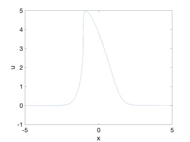
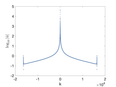
Figure 17. Solution to equation (1.1) with the $-$ sign for $\alpha=0.2$ for the initial data $u(x,0)=5\exp(-x^{2})$ at $t=0.0332$ on the left, and the corresponding Fourier coefficients on the right.

The above behavior is confirmed by various norms of the solution. In Fig. 18 it can be seen on the left that the $L^{\infty}$ norm of the solution is essentially constant and even decreases slightly. But the $L^{\infty}$ norm of the gradient on the right of the same figure appears to explode. This means both norms reflect the behavior of a shock of the solution.

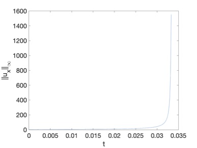
Figure 18. $L^{\infty}$ norm of the solution to equation (1.1) with the $-$ sign for $\alpha=0.2$ for the initial data $u(x,0)=5\exp(-x^{2})$ in dependence of time on the left, and the $L^{\infty}$ norm of the gradient on the right.

If we consider the same initial data for the defocusing equation (1.1) with $\alpha=0.1$, we get very similar results. The code is stopped for $t=0.033$ since the Fourier coefficients appear to show a completely algebraic decay for large $|k|$, and a fitting of the coefficients gives $\mu\sim 0.35$. The solution at this time can be seen in Fig. 19 on the left. The $L^{\infty}$ norm of the gradient in dependence of time on the right of the same figure again indicates a shock.

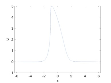
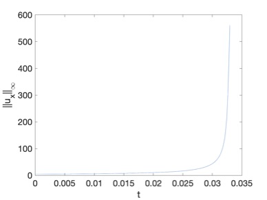
Figure 19. Solution to equation (1.1) with the $-$ sign for $\alpha=0.1$ for the initial data $u(x,0)=5\exp(-x^{2})$ for $t=0.033$ on the left, and the $L^{\infty}$ norm of the gradient on the right.

The above results can be summarized in the following

Conjecture 5.8.

Consider smooth initial data $u_{0}\in L^{2}(\mathbb{R})$ with a single hump for the defocusing equation (1.1). Then

• Initial data with sufficiently small mass will be dispersed, the solution is global in time.

• For $\alpha\geq 1/2$, initial data of arbitrary mass lead to solutions which will be dispersed and are global in time.

• For $\alpha<1/2$, initial data of sufficiently large mass will lead to the formation of a shock in finite time, a singularity of the form $|x-x^{*}|^{1/3}$ for $|x|\sim x^{*}$, where ${}^{*}=const$.

Remark 5.9.

The global existence and scattering for small solutions in the case $0<\alpha<1$ has been recently proven ([30]).

6. The BBM version

We comment here briefly on the BBM version of the modified fKdV equation, that is

$$u_{t}+u_{x}+|D|^{\alpha}u_{t}\pm u^{2}u_{x}=0,$$ (6.1)

which makes sense for $\alpha>0$, and we will restrict to $0<\alpha\leq 1.$

For any $\alpha>0$ the energy

$$E(t)=\frac{1}{2}\int_{\mathbb{R}}(u^{2}+|D^{\alpha/2}u|^{2})\,dx$$

is formally conserved. By a standard compactness method this implies that the Cauchy problem for (6.1) admits a global weak solution in $L^{\infty}(\mathbb{R}:H^{\alpha/2}(\mathbb{R}))$ for any initial data in $H^{\alpha/2}(\mathbb{R})$ when $\alpha>1/3$ (this condition ensures the compactness of the embedding $H^{\alpha/2}(\mathbb{R})\subset L^{3}_{\text{loc}}(\mathbb{R})$).

One can also use the equivalent form

$$\partial_{t}u+\partial_{x}(I+D^{\alpha})^{-1}\left(u\pm\frac{u^{3}}{3}\right)=0,$$

which gives the Hamiltonian formulation

$$u_{t}+J_{\alpha}\nabla_{u}H(u)=0,$$

where the skew-adjoint operator $J_{\alpha}$ is given by $J_{\alpha}=\partial_{x}(I+D^{\alpha})^{-1}$ and

$$H(u)=\frac{1}{2}\int_{\mathbb{R}}\bigg{(}u^{2}\pm\frac{1}{6}u^{4}\bigg{)}\,dx.$$

Note that the Hamiltonian $H(u)$ makes sense for $u\in H^{\alpha/2}(\mathbb{R})$ (due to the energy $E(t)$ and Sobolev embedding) if and only if $\alpha\geq 1/2$.

As noticed in [19] for the quadratic fBBM equation, when $\alpha\geq 1$ (6.1) is an ODE in the Sobolev space $H^{s}(\mathbb{R}),s>1/2$, which by standard arguments yields the local well-posedness of the Cauchy problem in $H^{s}(\mathbb{R}),s>1/2$. When $\alpha=1$ (the BBM version of the modified Benjamin-Ono equation), the conservation of energy and an ODE argument (see[27]) à la Brezis-Gallouet implies that this solution is in fact global.

The situation is more delicate when $0<\alpha<1.$ Concerning the local Cauchy problem, the local well-posedness in $H^{s}(\mathbb{R}),s>3/2$ is trivial. As in the quadratic case (see [19]) a local theory in $H^{3/2-s_{\alpha}}(\mathbb{R}),s_{\alpha}>0$ can be carried out but we will focus here on the global issues. Although the global existence of small solutions is expected, things are less clear for the behavior of large solutions (global existence versus finite time blow-up), and we will rely on numerical simulations, for $0<\alpha<1/3$ and $1/3<\alpha<1,$ for both signs in (6.1).

Equation (6.1) has solitary waves of the form $u(x,t)=\tilde{Q}(\xi)$, $\xi=x-ct$ satisfying

$$(1-c)\tilde{Q}-c|D|^{\alpha}\tilde{Q}\pm\frac{1}{3}\tilde{Q}^{3}=0.$$ (6.2)

One has for $c>1$ and the $+$ sign in (6.2)

$$\tilde{Q}(x)=\sqrt{c-1}Q(\beta^{1/\alpha}x),\quad\beta=\frac{c-1}{c},$$ (6.3)

where $Q$ is the solution of (5.1) for $c=1$, and for $c<-1$ and the $-$ sign in (6.2)

$$\tilde{Q}(x)=\sqrt{1-c}Q(\beta^{1/\alpha}x),\quad\beta=\frac{c-1}{c}.$$ (6.4)

Thus for equation (6.1) solitary waves are expected for both signs in front of the nonlinearity. They are propagating to the right for the $+$ sign, and to the left for the $-$ sign.

Remark 6.1.

We refer to [26] for a rather complete analysis of the stability of solitary waves to the fBBM equation:

$$u_{t}+u_{x}+|D|^{\alpha}u_{t}+uux=0.$$

For the numerical computations below we use $N=2^{16}$ Fourier modes for the shown domains in $x$ and $N_{t}=10^{4}$ time steps for the given time intervals. Note that in all cases discussed below, initial data of small enough mass are simply dispersed towards infinity. We do not show examples for this since they are very similar to what has been shown in this context before.

As a first example we address the case $\alpha=0.8$ where solitary waves are known to exist. We consider the initial data $u(x,0)=5\exp(-x^{2})$. The solution to (6.1) for the $+$ sign can be seen in Fig. 20. A larger solitary wave appears to form and is propagating to the right.

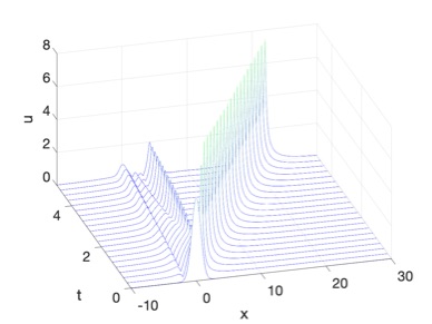
Figure 20. Solution to equation (6.1) with the $+$ sign for $\alpha=0.8$ for the initial data $u(x,0)=5\exp(-x^{2})$.

The $L^{\infty}$ norm of the solution on the left of Fig. 21 is in accordance with the interpretation that at least one large solitary wave appears. On the right of the same figure we show the solution at the final time together with a fitted solitary wave according to (6.3). It can be seen that the agreement is already excellent.

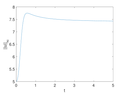
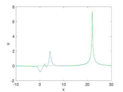
Figure 21. $L^{\infty}$ norm of the solution to equation (6.1) with the $+$ sign for $\alpha=0.8$ for the initial data $u(x,0)=5\exp(-x^{2})$ on the left, and the solution at the final time together with a fitted solitary wave according to (6.3) in green on the right.

The same initial data and $\alpha=0.8$ for the $-$ sign in (6.1) lead to the solution in Fig. 22. Again at least one solitary wave forms which travels to the left this time.

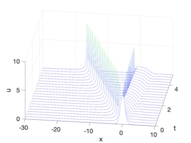
Figure 22. Solution to equation (6.1) with the $-$ sign for $\alpha=0.8$ for the initial data $u(x,0)=5\exp(-x^{2})$.

This is once more confirmed by the $L^{\infty}$ norm of the solution on the left of Fig. 23, and even more so by the solution at the final time on the right of the same figure together with a fitted solitary wave according to (6.4). This shows that the soliton resolution conjecture applies to both the equation (6.1) with the plus and the minus sign. In particular this implies that the solitons are stable for $\alpha>0.5$.

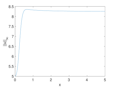
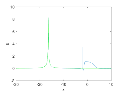
Figure 23. $L^{\infty}$ norm of the solution to equation (6.1) with the $-$ sign for $\alpha=0.8$ for the initial data $u(x,0)=5\exp(-x^{2})$ on the left, and the solution at the final time together with a fitted solitary wave according to (6.4) in green on the right.

For $0<\alpha<1/3$, we consider as an example $\alpha=0.2$ and the initial data $u(x,0)=\exp(-x^{2})$. We find that the code breaks for $t=2.5713$ since a fit of the Fourier coefficients according to (2.55) indicates the formation of a singularity with $\mu\sim 0.19$. The solution at this time can be seen in Fig. 24 on the left. The $L^{\infty}$ norm of the solution in dependence of time is shown on the right of the same figure. It grows until the code breaks, but as mentioned the Fourier coefficients indicate that a cusp appears at this time with finite $L^{\infty}$ norm. This is similar to what was observed for the fBBM equation in [18].

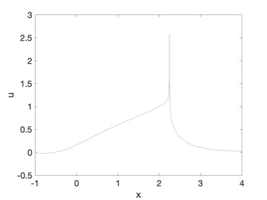
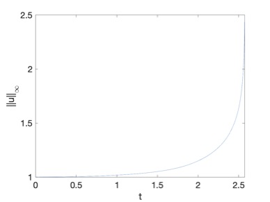
Figure 24. Solution to equation (6.1) with the $+$ sign for $\alpha=0.2$ for the initial data $u(x,0)=\exp(-x^{2})$ for $t=2.5713$ on the left, and the $L^{\infty}$ norm in dependence of time on the right.

The situation for the same initial data is different in the case of (6.1) with the $-$ sign. Here we get a dispersive shock wave as can be seen in Fig. 25. There is no indication of the formation of a singularity in this case.

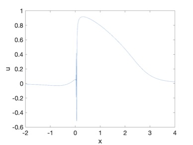
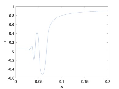
Figure 25. Solution to equation (6.1) with the $-$ sign for $\alpha=0.2$ for the initial data $u(x,0)=\exp(-x^{2})$ for $t=3$ on the left, and a close-up of the DSW on the right.

However, for initial data with slightly larger norm, the situation is as in the focusing case in Fig. 24. If we consider the initial data $u(x,0)=1.5\exp(-x^{2)}$, then the code breaks for $t=1.0174$ since a fitting of the Fourier coefficients according to (2.55) indicates a cusp ($\mu\sim 0.17$). The solution for $t=1.014$ can be seen on the left of Fig. 26. The $L^{\infty}$ norm of the gradient on the right of the same figure also indicates the formation of a cusp.

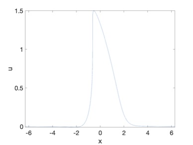
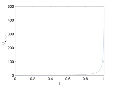
Figure 26. Solution to equation (6.1) with the $-$ sign for $\alpha=0.2$ for the initial data $u(x,0)=1.5\exp(-x^{2})$ for $t=1.014$ on the left, and the $L^{\infty}$ norm of $u_{x}$ in dependence of time on the right.

The above results can be summarized in the following

Conjecture 6.2.

Consider smooth initial data $u_{0}\in L^{2}(\mathbb{R})$ with a single hump for the equation (6.1). Then

• Initial data of sufficiently small mass will be dispersed, the solutions are global in time for $0<\alpha<1$.

• For $\alpha\geq 1/3$, the solutions are global in time.

• For $\alpha>1/2$ the long time behavior of initial data of sufficiently large mass is characterized by solitary waves and radiation.

• For $\alpha<1/3$, initial data of sufficiently large mass can lead to the formation of a cusp in finite time.

Acknowledgments. This work was partially supported by the ANR project ANuI (ANR-17-CE40-0035-02). CK’s work is partially supported by the isite BFC project NAANoD, the EIPHI Graduate School (contract ANR-17-EURE-0002), by the European Union Horizon 2020 research and innovation program under the Marie Sklodowska-Curie RISE 2017 grant agreement no. 778010 IPaDEGAN, and the EITAG project funded by the FEDER de Bourgogne, the region Bourgogne-Franche-Comté and the EUR EIPHI.

References

- [1] M.A. Alejo and C. Munoz, Nonlinear stability of MKdV breathers, Commun. Math. Phys. 324 (2013), 233-262.
- [2] J. Biello and J. Hunter, Nonlinear Hamiltonian waves with constant frequency and surface waves on vorticity discontinuity, Comm. Pure Appl. Math., 63 (2009), 303-336.
- [3] A. Castro, D. Córdoba and F. Gancedo, Singularity formation in a surface wave model, Nonlinearity, 23 (2010), 2835-2847.
- [4] A. Constantin and J. Escher, Wave breaking for nonlinear nonlocal shallow water equations, Acta Math., 181 (1998), 229-245.
- [5] M.Ehrnström and E. Wahlén, On Whitham’s conjecture of a highest cusped wave for a nonlocal shallow water wave equation, Ann. Inst. H. Poincaré Anal. Non Linéaire, 36 (2019), 1603-1637.
- [6] M.Ehrnström and Y. Wang, Enhanced existence time of solutions to the fractional Korteweg-de Vries equation, SIAM J. Math. Anal., 51 (2019), 3298-3323.
- [7] M.Ehrnström and Y. Wang, Enhanced existence time of solutions to evolution equations of Whitham type, arXiv:2008.12722, (2020).
- [8] R.L. Frank and E. Lenzmann, On the uniqueness and nondegeneracy of ground states of , Acta Math., 210 (2) (2013), 261-318.
- [9] V. Hur and L. Tao, Wave breaking for the Whitham equation with fractional dispersion, Nonlinearity, 27 (2014), 2937-2949.
- [10] V. Hur, Wave breaking in the Whitham equation, Adv. Math., 317 (2017), 410-437.
- [11] C. Klein, F. Linares, D. Pilod and J.-C. Saut, On Whitham and related equations, Studies in Appl. Math., 140 (2018), 133-177.
- [12] C. Klein and R. Peter, Numerical study of blow-up in solutions to generalized Korteweg-de Vries equations, Phys. D, 304-305 (2015), 52-78.
- [13] C.E. Kenig and K.D. Koenig, On the local well-posedness of the Benjamin-Ono and modified Benjamin-Ono equations, Math. Res. Letters, 10 (2003), 879-895.
- [14] C.E. Kenig, Y. Martel and L. Robbiano, Local well-posedness and blow-up in the energy space for a class of critical dispersion generalized Benjamin-Ono equations, Ann. Inst. H. Poincaré Anal. Non Linéaire, 28 (2011), 853-887.
- [15] C.E. Kenig and T. Takaoka, Global well-posedness of the modified Benjamin-Ono equation with initial data in , Int. Math. Res. Not., 2006 (2006), 1-44.
- [16] C. Klein, K. Roidot, Numerical study of shock formation in the dispersionless Kadomtsev- Petviashvili equation and dispersive regularizations, Phys. D, 265 (2013), https://doi.org/10.1016/j.physd.2013.09.005.
- [17] C. Klein, C. Sparber and P. Markowich, Numerical study of fractional Nonlinear Schrödinger equations, Proc. R. Soc. A 470: 20140364, http://doi.org/10.1098/rspa.2014.0364.
- [18] C. Klein, and J.-C. Saut, A numerical approach to blow-up issues for dispersive perturbations of Burgers’ equation, Phys. D, 295/296 (2015), 46-65.
- [19] F. Linares, D. Pilod, and J.-C. Saut, Dispersive perturbations of Burgers and hyperbolic equations I: local theory, SIAM J. Math. Anal., 46 (2014), 1505-1537.
- [20] F. Linares, D. Pilod and J.-C. Saut, Remarks on the orbital stability of ground state solutions of fKdV and related equations, Adv. Differ. Equ., 20 (9/10), (2015), 835-858.
- [21] Y. Martel and D. Pilod, Construction of a minimal mass blow-up solution to the modified Benjamin-Ono equation, Math. Annal., 369 (1-2) (2017), 153-245.
- [22] A.J. Mendez, On the propagation of regularity for solutions of fractional Korteweg-de Vries equations, J. Differ. Equ., 269 (2020), 9051-9O89.
- [23] L. Molinet, D. Pilod and S. Vento, On well-posedness for some dispersive perturbations of the Burgers equation, Ann. Inst. H. Poincaré Anal. Non Linéaire, 35 (2018), 1719-1756.
- [24] L. Molinet and F. Ribaud, Well-posedness for the generalized Benjamin-Ono equation with arbitrary large initial data, Int. Math. Res. Not., 70 (204), 3757-3795.
- [25] P. I. Naumkin and I. A. Shishmarëv, Nonlinear nonlocal equations in the theory of waves, Translations of Mathematical Monographs 133 (1994), American Mathematical Society, Providence, RI, Translated from the Russian manuscript by Boris Gommerstadt.
- [26] J. A. Pava, Stability properties of solitary waves for fractional KdV and BBM equation, Nonlinearity 31 (2018), 920-956.
- [27] J.-C.Saut, Sur quelques généralisations de l’équation de KdV I, J. Math. Pures Appl. 58 (1979), 21-61.
- [28] J.-C. Saut and Y. Wang, Long time behavior of the fractional Korteweg-de Vries equation with cubic nonlinearity, Discrete Contin. Dyn. Syst., https://doi.org/10.3934/dcds.2020312, arXiv:2003.05910, (2020).
- [29] J.-C. Saut and Y. Wang, The wave breaking for Whitham-type equations revisited, arXiv:2006.03803, (2020).
- [30] J.-C. Saut and Y. Wang, In preparation.
- [31] C. Sulem, P. Sulem, and H. Frisch, Tracing complex singularities with spectral methods, J. Comp. Phys., 50 (1983), 138-161.
- [32] G.B. Whitham, Linear and nonlinear waves, Wiley, New York 1974.
- [33] G. B. Whitham, Variational methods and applications to water waves, Proc.R. Soc. Lond. Ser. A., 299 (1967), 6-25.