Adaptive Aggregation Networks for Class-Incremental Learning

Abstract

Class-Incremental Learning (CIL) aims to learn a classification model with the number of classes increasing phase-by-phase. An inherent problem in CIL is the stability-plasticity dilemma between the learning of old and new classes, i.e., high-plasticity models easily forget old classes, but high-stability models are weak to learn new classes. We alleviate this issue by proposing a novel network architecture called Adaptive Aggregation Networks (AANets) in which we explicitly build two types of residual blocks at each residual level (taking ResNet as the baseline architecture): a stable block and a plastic block. We aggregate the output feature maps from these two blocks and then feed the results to the next-level blocks. We adapt the aggregation weights in order to balance these two types of blocks, i.e., to balance stability and plasticity, dynamically. We conduct extensive experiments on three CIL benchmarks: CIFAR-100, ImageNet-Subset, and ImageNet, and show that many existing CIL methods can be straightforwardly incorporated into the architecture of AANets to boost their performances.

1 Introduction

AI systems are expected to work in an incremental manner when the amount of knowledge increases over time. They should be capable of learning new concepts while maintaining the ability to recognize previous ones. However, deep-neural-network-based systems often suffer from serious forgetting problems (called “catastrophic forgetting”) when they are continuously updated using new coming data. This is due to two facts: (i) the updates can override the knowledge acquired from the previous data [27, 28, 33, 40, 19], and (ii) the model can not replay the entire previous data to regain the old knowledge.

To encourage solving these problems, [34] defined a class-incremental learning (CIL) protocol for image classification where the training data of different classes gradually come phase-by-phase. In each phase, the classifier is re-trained on new class data, and then evaluated on the test data of both old and new classes. To prevent trivial algorithms such as storing all old data for replaying, there is a strict memory budget due to which a tiny set of exemplars of old classes can be saved in the memory. This memory constraint causes a serious data imbalance problem between old and new classes, and indirectly causes the main problem of CIL – the stability-plasticity dilemma [29]. In particular, higher plasticity results in the forgetting of old classes [27], while higher stability weakens the model from learning the data of new classes (that contain a large number of samples). Existing CIL works try to balance stability and plasticity using data strategies. For example, as illustrated in Figure 1 (a) and (b), some early methods train their models on the imbalanced dataset where there is only a small set of exemplars for old classes [34, 23], and recent methods include a fine-tuning step using a balanced subset of exemplars sampled from all classes [4, 16, 11]. However, these data strategies are still limited in terms of effectiveness. For example, when using the models trained after $25$ phases, LUCIR [16] and Mnemonics [25] “forget” the initial $50$ classes by $30\%$ and $20\%$, respectively, on the ImageNet dataset [37].

In this paper, we address the stability-plasticity dilemma by introducing a novel network architecture called Adaptive Aggregation Networks (AANets). Taking the ResNet [14] as an example of baseline architectures, we explicitly build two residual blocks (at each residual level) in AANets: one for maintaining the knowledge of old classes (i.e., the stability) and the other for learning new classes (i.e., the plasticity), as shown in Figure 1 (c). We achieve these by allowing these two blocks to have different levels of learnability, i.e., less learnable parameters in the stable block but more in the plastic one. We apply aggregation weights to the output feature maps of these blocks, sum them up, and pass the result maps to the next residual level. In this way, we are able to dynamically balance the usage of these blocks by updating their aggregation weights. To achieve auto-updating, we take the weights as hyperparameters and optimize them in an end-to-end manner [12, 48, 25].

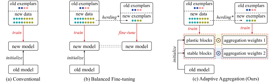
Figure 1: Conceptual illustrations of different CIL methods. (a) Conventional methods use all available data (which are imbalanced among classes) to train the model [34, 16] (b) Recent methods [4, 16, 11, 25] follow this convention but add a fine-tuning step on a balanced subset of all classes. (c) The proposed Adaptive Aggregation Networks (AANets) is a new architecture and it applies a different data strategy: using all available data to update the parameters of plastic and stable blocks, and the balanced set of exemplars to adapt the aggregation weights for these blocks. Our key lies in that adapted weights can balance the usage of the plastic and stable blocks, i.e., balance between plasticity and stability. *: herding is the method to choose exemplars [47], and can be replaced by others, e.g., mnemonics training in [25]. We highlight that in the implementation of AANets, we strictly control the memory (i.e., the sizes of input data and residual blocks) within the same budget as the other methods. Please refer to the details in the section of experiments.

Technically, the overall optimization of AANets is bilevel. Level-1 is to learn the network parameters for two types of residual blocks, and level-2 is to adapt their aggregation weights. More specifically, level-1 is the standard optimization of network parameters, for which we use all the data available in the phase. Level-2 aims to balance the usage of the two types of blocks, for which we optimize the aggregation weights using a balanced subset (by downsampling the data of new classes), as illustrated in Figure 1 (c). We formulate these two levels in a bilevel optimization program (BOP) [41] that solves two optimization problems alternatively, i.e., update network parameters with aggregation weights fixed, and then switch. For evaluation, we conduct CIL experiments on three widely-used benchmarks, CIFAR-100, ImageNet-Subset, and ImageNet. We find that many existing CIL methods, e.g., iCaRL [34], LUCIR [16], Mnemonics Training [25], and PODNet [11], can be directly incorporated in the architecture of AANets, yielding consistent performance improvements. We observe that a straightforward plug-in causes memory overheads, e.g., $26\%$ and $15\%$ respectively for CIFAR-100 and ImageNet-Subset. For a fair comparison, we conduct additional experiments under the settings of zero overhead (e.g., by reducing the number of old exemplars for training AANets), and validate that our approach still achieves top performance across all datasets.

Our contribution is three-fold: 1) a novel and generic network architecture called AANets specially designed for tackling the stability-plasticity dilemma in CIL tasks; 2) a BOP-based formulation and an end-to-end training solution for optimizing AANets; and 3) extensive experiments on three CIL benchmarks by incorporating four baseline methods in the architecture of AANets.

2 Related Work

Incremental learning aims to learn efficient machine models from the data that gradually come in a sequence of training phases. Closely related topics are referred to as continual learning [10, 26] and lifelong learning [7, 2, 22]. Recent incremental learning approaches are either task-based, i.e., all-class data come but are from a different dataset for each new phase [23, 40, 17, 6, 35, 54, 8, 5], or class-based i.e., each phase has the data of a new set of classes coming from the identical dataset [34, 16, 48, 4, 25, 18, 53]. The latter one is typically called class-incremental learning (CIL), and our work is based on this setting. Related methods mainly focus on how to solve the problems of forgetting old data. Based on their specific methods, they can be categorized into three classes: regularization-based, replay-based, and parameter-isolation-based [9, 30].
Regularization-based methods introduce regularization terms in the loss function to consolidate previous knowledge when learning new data. Li et al. [23] proposed the regularization term of knowledge distillation [15]. Hou et al. [16] introduced a series of new regularization terms such as for less-forgetting constraint and inter-class separation to mitigate the negative effects caused by the data imbalance between old and new classes. Douillard et al. [11] proposed an effective spatial- based distillation loss applied throughout the model and also a representation comprising multiple proxy vectors for each object class. Tao et al. [44] built the framework with a topology-preserving loss to maintain the topology in the feature space. Yu et al. [51] estimated the drift of previous classes during the training of new classes.
Replay-based methods store a tiny subset of old data, and replay the model on them (together with new class data) to reduce the forgetting. Rebuffi et al. [34] picked the nearest neighbors to the average sample per class to build this subset. Liu et al. [25] parameterized the samples in the subset, and then meta-optimized them automatically in an end-to-end manner taking the representation ability of the whole set as the meta-learning objective. Belouadah et al. [3] proposed to leverage a second memory to store statistics of old classes in rather compact formats.
Parameter-isolation-based methods are used in task-based incremental learning (but not CIL). Related methods dedicate different model parameters for different incremental phases, to prevent model forgetting (caused by parameter overwritten). If no constraints on the size of the neural network is given, one can grow new branches for new tasks while freezing old branches. Rusu et al. [38] proposed “progressive networks” to integrate the desiderata of different tasks directly into the networks. Abati et al. [1] equipped each convolution layer with task-specific gating modules that select specific filters to learn each new task. Rajasegaran et al.[31] progressively chose the optimal paths for the new task while encouraging to share parameters across tasks. Xu et al. [49] searched for the best neural network architecture for each coming task by leveraging reinforcement learning strategies. Our differences with these methods include the following aspects. We focus on class-incremental learning, and more importantly, our approach does not continuously increase the network size. We validate in the experiments that under a strict memory budget, our approach can surpass many related methods and its plug-in versions on these related methods can bring consistent performance improvements.

Bilevel Optimization Program can be used to optimize hyperparameters of deep models. Technically, the network parameters are updated at one level and the key hyperparameters are updated at another level [45, 46, 13, 52, 24, 21]. Recently, a few bilevel-optimization-based approaches have emerged for tackling incremental learning tasks. Wu et al. [48] learned a bias correction layer for incremental learning models using a bilevel optimization framework. Rajasegaran et al. [32] incrementally learned new tasks while learning a generic model to retain the knowledge from all tasks. Riemer et al. [36] learned network updates that are well-aligned with previous phases, such as to avoid learning towards any distracting directions. In our work, we apply the bilevel optimization program to update the aggregation weights in our AANets.

3 Adaptive Aggregation Networks (AANets)

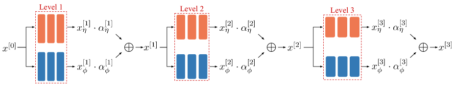
Figure 2: An example architecture of AANets with three levels of residual blocks. At each level, we compute the feature maps from a stable block ($\phi\odot\theta_{\mathrm{base}}$, blue) as well as a plastic block ($\eta$, orange), respectively, aggregate the maps with adapted weights, and feed the result maps to the next level. The outputs of the final level are used to train classifiers. We highlight that this is a logical architecture of AANets, and in real implementations, we strictly control the memory (i.e., the sizes of input data and residual blocks) within the same budget as related works which deploy plain ResNets. Please refer to the details in the section of experiments.

Class-Incremental Learning (CIL) usually assumes $(N+1)$ learning phases in total, i.e., one initial phase and $N$ incremental phases during which the number of classes gradually increases [16, 25, 11, 18]. In the initial phase, data $\mathcal{D}_{0}$ is available to train the first model $\Theta_{0}$. There is a strict memory budget in CIL systems, so after the phase, only a small subset of $\mathcal{D}_{0}$ (exemplars denoted as $\mathcal{E}_{0}$) can be stored in the memory and used as replay samples in later phases. Specifically in the $i$-th ($i\geq 1$) phase, we load the exemplars of old classes $\mathcal{E}_{0:i-1}=\{\mathcal{E}_{0},\dots,\mathcal{E}_{i-1}\}$ to train model $\Theta_{i}$ together with new class data $\mathcal{D}_{i}$. Then, we evaluate the trained model on the test data containing both old and new classes. We repeat such training and evaluation through all phases.

The key issue of CIL is that the models trained at new phases easily “forget” old classes. To tackle this, we introduce a novel architecture called AANets. AANets is based on a ResNet-type architecture, and each of its residual levels is composed of two types of residual blocks: a plastic one to adapt to new class data and a stable one to maintain the knowledge learned from old classes. The details of this architecture are elaborated in Section 3.1. The steps for optimizing AANets are given in Section 3.2.

3.1 Architecture Details

In Figure 2, we provide an illustrative example of our AANets with three residual levels. The inputs $x^{[0]}$ are the images and the outputs $x^{[3]}$ are the features used to train classifiers. Each of our residual “levels” consists of two parallel residual “blocks” (of the original ResNet [14]): the orange one (called plastic block) will have its parameters fully adapted to new class data, while the blue one (called stable block) has its parameters partially fixed in order to maintain the knowledge learned from old classes. After feeding the inputs to Level 1, we obtain two sets of feature maps respectively from two blocks, and aggregate them after applying the aggregation weights $\alpha^{[1]}$. Then, we feed the resulted maps to Level 2 and repeat the aggregation. We apply the same steps for Level 3. Finally, we pool the resulted maps obtained from Level 3 to train classifiers. Below we elaborate the details of this dual-branch design as well as the steps for feature extraction and aggregation.

Stable and Plastic Blocks. We deploy a pair of stable and plastic blocks at each residual level, aiming to balance between the plasticity, i.e., for learning new classes, and stability, i.e., for not forgetting the knowledge of old classes. We achieve these two types of blocks by allowing different levels of learnability, i.e., less learnable parameters in the stable block but more in the plastic. We detail the operations in the following. In any CIL phase, Let $\eta$ and $\phi$ represent the learnable parameters of plastic and stable blocks, respectively. $\eta$ contains all the convolutional weights, while $\phi$ contains only the neuron-level scaling weights [43]. Specifically, these scaling weights are applied on the model $\theta_{\mathrm{base}}$ obtained in the $0$-th phase. As a result, the number of learnable parameters $\phi$ is much less than that of $\eta$. For example, when using $3\times 3$ neurons in $\theta_{\mathrm{base}}$, the number of learnable parameters $\phi$ is only $\frac{1}{3\times 3}$ of the number of full network parameters (while $\eta$ has the full network parameters). We further elaborate on these in the following paragraph.

Neuron-level Scaling Weights. For stable blocks, we learn its neuron parameters in the $0$-th phase and freeze them in the other $N$ phases. In these $N$ phases, we apply a small set of scaling weights $\phi$ at the neuron-level, i.e., each weight for scaling one neuron in $\theta_{\mathrm{base}}$. We aim to preserve the structural pattern within the neuron and slowly adapt the knowledge of the whole blocks to new class data. Specifically, we assume the $q$-th layer of $\theta_{\mathrm{base}}$ contains $R$ neurons, so we have $R$ neuron weights as $\{W_{q,r}\}_{r=1}^{R}$. For conciseness, we denote them as $W_{q}$. For $W_{q}$, we learn $R$ scaling weights denoted as $\phi_{q}$ Let $X_{q-1}$ and $X_{q}$ be the input and output feature maps of the $q$-th layer, respectively. We apply $\phi_{q}$ to $W_{q}$ as follows,

$$X_{q}=(W_{q}\odot\phi_{q})X_{q-1},$$ (1)

where $\odot$ donates the element-wise multiplication. Assuming there are $Q$ layers in total, the overall scaling weights can be denoted as $\phi=\{\phi_{q}\}_{q=1}^{Q}$.

Feature Extraction and Aggregation. We elaborate on the process of feature extraction and aggregation across all residual levels in the AANets, as illustrated in Figure 2. Let $\mathcal{F}^{[k]}_{\mu}{(\cdot)}$ denote the transformation function of the residual block parameterized as $\mu$ at the Level $k$. Given a batch of training images $x^{[0]}$, we feed them to AANets to compute the feature maps at the $k$-th level (through the stable and plastic blocks respectively) as follows,

$$x_{\phi}^{[k]}=\mathcal{F}^{[k]}_{\phi\odot\theta_{\mathrm{base}}}(x^{[k-1]});\quad x_{\eta}^{[k]}=\mathcal{F}^{[k]}_{\eta}(x^{[k-1]}).$$ (2)

The transferability (of the knowledge learned from old classes) is different at different levels of neural networks [50]. Therefore, it makes more sense to apply different aggregation weights for different levels of residual blocks. Let $\alpha^{[k]}_{\phi}$ and $\alpha^{[k]}_{\eta}$ denote the aggregation weights of the stable and plastic blocks, respectively, at the $k$-th level. Then, the weighted sum of $x_{\phi}^{[k]}$ and $x_{\eta}^{[k]}$ can be derived as follows,

$$x^{[k]}=\alpha^{[k]}_{\phi}\cdot x_{\phi}^{[k]}+\alpha^{[k]}_{\eta}\cdot x_{\eta}^{[k]}.$$ (3)

In our illustrative example in Figure 2, there are three pairs of weights to learn at each phase. Hence, it becomes increasingly challenging to choose these weights manually if multiple phases are involved. In this paper, we propose an learning strategy to automatically adapt these weights, i.e., optimizing the weights for different blocks in different phases, see details in Section 3.2.

3.2 Optimization Steps

In each incremental phase, we optimize two groups of learnable parameters in AANets: (a) the neuron-level scaling weights $\phi$ for the stable blocks and the convolutional weights $\eta$ on the plastic blocks; (b) the feature aggregation weights $\alpha$. The former is for network parameters and the latter is for hyperparameters. In this paper, we formulate the overall optimization process as a bilevel optimization program (BOP) [13, 25].

The Formulation of BOP. In AANets, the network parameters $[\phi,\eta]$ are trained using the aggregation weights $\alpha$ as hyperparameters. In turn, $\alpha$ can be updated when temporarily fixing network parameters $[\phi,\eta]$. In this way, the optimality of $[\phi,\eta]$ imposes a constraint on $\alpha$ and vise versa. Ideally, in the $i$-th phase, the CIL system aims to learn the optimal $\alpha_{i}$ and $[\phi_{i},\eta_{i}]$ that minimize the classification loss on all training samples seen so far, i.e., $\mathcal{D}_{i}\cup\mathcal{D}_{0:i-1}$, so the ideal BOP can be formulated as,

$$\min_{\alpha_{i}}\mathcal{L}(\alpha_{i},\phi^{*}_{i},\eta^{*}_{i};\mathcal{D}_{0:i-1}\cup\mathcal{D}_{i})$$ (4a)

$$\ \text{s.t.}\ [\phi_{i}^{*},\eta^{*}_{i}]=\operatorname*{arg\,min}_{[\phi_{i},\eta_{i}]}\mathcal{L}(\alpha_{i},\phi_{i},\eta_{i};\mathcal{D}_{0:i-1}\cup\mathcal{D}_{i}),$$ (4b)

where $\mathcal{L}(\cdot)$ denotes the loss function, e.g., cross-entropy loss. Please note that for the conciseness of the formulation, we use $\phi_{i}$ to represent $\phi_{i}\odot\theta_{\mathrm{base}}$ (same in the following equations). We call Problem 4a and Problem 4b the upper-level and lower-level problems, respectively.

Data Strategy. To solve Problem 4, we need to use $\mathcal{D}_{0:i-1}$. However, in the setting of CIL [34, 16, 11], we cannot access $\mathcal{D}_{0:i-1}$ but only a small set of exemplars $\mathcal{E}_{0:i-1}$, e.g., $20$ samples of each old class. Directly replacing $\mathcal{D}_{0:i-1}\cup\mathcal{D}_{i}$ with $\mathcal{E}_{0:i-1}\cup\mathcal{D}_{i}$ in Problem 4 will lead to the forgetting problem for the old classes. To alleviate this issue, we propose a new data strategy in which we use different training data splits to learn different groups of parameters: 1) in the upper-level problem, $\alpha_{i}$ is used to balance the stable and the plastic blocks, so we use the balanced subset to update it, i.e., learning $\alpha_{i}$ on $\mathcal{E}_{0:i-1}\cup\mathcal{E}_{i}$ adaptively; 2) in the lower-level problem, $[\phi_{i},\eta_{i}]$ are the network parameters used for feature extraction, so we leverage all the available data to train them, i.e., base-training $[\phi_{i},\eta_{i}]$ on $\mathcal{E}_{0:i-1}\cup\mathcal{D}_{i}$. Based on these, we can reformulate the ideal BOP in Problem 4 as a solvable BOP as follows,

$$\min_{\alpha_{i}}\mathcal{L}(\alpha_{i},\phi^{*}_{i},\eta^{*}_{i};\mathcal{E}_{0:i-1}\cup\mathcal{E}_{i})$$ (5a)

$$\ \text{s.t.}\ [\phi_{i}^{*},\eta^{*}_{i}]=\operatorname*{arg\,min}_{[\phi_{i},\eta_{i}]}\mathcal{L}(\alpha_{i},\phi_{i},\eta_{i};\mathcal{E}_{0:i-1}\cup\mathcal{D}_{i}),$$ (5b)

where Problem 5a is the upper-level problem and Problem 5b is the lower-level problem we are going to solve.

Updating Parameters. We solve Problem 5 by alternatively updating two groups of parameters ($\alpha_{i}$ and $[\phi,\eta]$) across epochs, e.g., if $\alpha_{i}$ is updated in the $j$-th epoch, then $[\phi,\eta]$ will be updated in the $(j+1)$-th epoch, until both of them converge. Taking the $i$-th phase as an example, we initialize ${\alpha}_{i},\phi_{i},\eta_{i}$ with ${\alpha}_{i-1},\phi_{i-1},\eta_{i-1}$, respectively. Please note that $\phi_{0}$ is initialized with ones, following [43, 42]; $\eta_{0}$ is initialized with $\theta_{\mathrm{base}}$; and ${\alpha}_{0}$ is initialized with $0.5$. Based on our Data Strategy, we use all available data in the current phase to solve the lower-level problem, i.e., training [$\phi_{i}$, $\eta_{i}$] as follows,

$$[\phi_{i},\eta_{i}]\leftarrow[\phi_{i},\eta_{i}]-\gamma_{1}\nabla_{[\phi_{i},\eta_{i}]}\mathcal{L}(\alpha_{i},\phi_{i},\eta_{i};\mathcal{E}_{0:i-1}\cup\mathcal{D}_{i}).$$ (6)

Then, we use a balanced exemplar set to solve the upper-level problem, i.e., training ${\alpha}_{i}$ as follows,

$${\alpha}_{i}\leftarrow{\alpha}_{i}-\gamma_{2}\nabla_{{\alpha}_{i}}\mathcal{L}({\alpha}_{i},\phi_{i},\eta_{i};\mathcal{E}_{0:i-1}\cup\mathcal{E}_{i}),$$ (7)

where $\gamma_{1}$ and $\gamma_{2}$ are the lower-level and upper-level learning rates, respectively.

Input: New class data $\mathcal{D}_{i}$; old class exemplars $\mathcal{E}_{0:i-1}$; old parameters $\alpha_{i-1}$, $\phi_{i-1}$, $\eta_{i-1}$; base model $\theta_{\mathrm{base}}$.

Output: new parameters $\alpha_{i}$, $\phi_{i}$, $\eta_{i}$; new class exemplars $\mathcal{E}_{i}$.

1

2Get $\mathcal{D}_{i}$ and load $\mathcal{E}_{0:i-1}$ from memory;

3 Initialize $[\phi_{i},\eta_{i}]$ with $[\phi_{i-1},\eta_{i-1}]$;

4 Initialize $\alpha_{i}$ with $\alpha_{i-1}$;

5 Select exemplars $\mathcal{E}_{i}\subsetneqq\mathcal{D}_{i}$, e.g. by herding [34, 16] or mnemonics training [25];

6 for epochs do

7       for mini-batches in $\mathcal{E}_{0:i-1}\cup\mathcal{D}_{i}$ do

8             Train $[\phi_{i},\eta_{i}]$ on $\mathcal{E}_{0:i-1}\cup\mathcal{D}_{i}$ by Eq. 6;

9            

10       end for

11      for mini-batches in $\mathcal{E}_{0:i-1}\cup\mathcal{E}_{i}$ do

12             Learn ${\alpha}_{i}$ on $\mathcal{E}_{0:i-1}\cup\mathcal{E}_{i}$ by Eq. 7;

13            

14       end for

15      

16 end for

17Update exemplars $\mathcal{E}_{i}$, e.g. by herding [34, 16] or mnemonics training [25];

Replace $\mathcal{E}_{0:i-1}$ with $\mathcal{E}_{0:i-1}\cup\mathcal{E}_{i}$ in the memory.

Algorithm 1 AANets (in the $i$-th phase)

3.3 Algorithm

In Algorithm 1, we summarize the overall training steps of the proposed AANets in the $i$-th incremental learning phase (where $i\in[1,...,N]$). Lines 1-4 show the preprocessing including loading new data and old exemplars (Line 1), initializing the two groups of learnable parameters (Lines 2-3), and selecting the exemplars for new classes (Line 4). Lines 5-12 optimize alternatively between the network parameters and the Adaptive Aggregation weights. In specific, Lines 6-8 and Lines 9-11 execute the training for solving the upper-level and lower-level problems, respectively. Lines 13-14 update the exemplars and save them to the memory.

4 Experiments

We evaluate the proposed AANets on three CIL benchmarks, i.e., CIFAR-100 [20], ImageNet-Subset [34] and ImageNet [37]. We incorporate AANets into four baseline methods and boost their model performances consistently for all settings. Below we describe the datasets and implementation details (Section 4.1), followed by the results and analyses (Section 4.2) which include a detailed ablation study, extensive comparisons to related methods, and some visualization of the results.

4.1 Datasets and Implementation Details

Row		Ablation Setting				CIFAR-100 (acc.%)							ImageNet-Subset (acc.%)
						Memory	FLOPs	#Param	$N$=5	10	25		Memory	FLOPs	#Param	$N$=5	10	25
1	single-branch “all” [16]					7.64MB	70M	469K	63.17	60.14	57.54		330MB	1.82G	11.2M	70.84	68.32	61.44
2	“all” + “all”					9.43MB	140M	938K	64.49	61.89	58.87		372MB	3.64G	22.4M	69.72	66.69	63.29
3	“all” + “scaling”					9.66MB	140M	530K	66.74	65.29	63.50		378MB	3.64G	12.6M	72.55	69.22	67.60
4	“all” + “frozen”					9.43MB	140M	469K	65.62	64.05	63.67		372MB	3.64G	11.2M	71.71	69.87	67.92
5	“scaling” + “frozen”					9.66MB	140M	60K	64.71	63.65	62.89		378MB	3.64G	1.4M	73.01	71.65	70.30
6	w/o balanced $\mathcal{E}$					9.66MB	140M	530K	65.91	64.70	63.08		378MB	3.64G	12.6M	70.30	69.92	66.89
7	w/o adapted $\alpha$					9.66MB	140M	530K	65.89	64.49	62.89		378MB	3.64G	12.6M	70.31	68.71	66.34
8	strict memory budget					7.64MB	140M	530K	66.46	65.38	61.79		330MB	3.64G	12.6M	72.21	69.10	67.10

Table 1: Ablation study. The baseline (Row 1) is LUCIR [16]. “all”, “scaling”, and “frozen” denote three types of blocks and they have different numbers of learnable parameters, e.g., “all” means all convolutional weights and biases are learnable. If we name them as A, B, and C, we use A+B in the table to denote the setting of using A-type and B-type blocks respectively as plastic and stable blocks. See more details in Section 4.2 Ablation settings. Adapted ${\alpha}$ are applied on Rows 3-8. “all”+“scaling” is the default setting of Rows 6-8. “#Param” indicates the number of learnable parameters. “Memory” denotes the peak memory for storing the exemplars and the learnable & frozen network parameters during the model training through all phases. Please refer to more results in the supplementary materials.

Datasets. We conduct CIL experiments on two datasets, CIFAR-100 [20] and ImageNet [37], following closely related work [16, 25, 11]. CIFAR-100 contains $60,000$ samples of $32\times 32$ color images for $100$ classes. There are $500$ training and $100$ test samples for each class. ImageNet contains around $1.3$ million samples of $224\times 224$ color images for $1000$ classes. There are approximately $1,300$ training and $50$ test samples for each class. ImageNet is used in two CIL settings: one based on a subset of $100$ classes (ImageNet-Subset) and the other based on the full set of $1,000$ classes. The $100$-class data for ImageNet-Subset are sampled from ImageNet in the same way as [16, 11].

Architectures. Following the exact settings in [16, 25], we deploy a $32$-layer ResNet as the baseline architecture (based on which we build the AANets) for CIFAR-100. This ResNet consists of $1$ initial convolution layer and $3$ residual blocks (in a single branch). Each block has $10$ convolution layers with $3\times 3$ kernels. The number of filters starts from $16$ and is doubled every next block. After these $3$ blocks, there is an average-pooling layer to compress the output feature maps to a feature embedding. To build AANets, we convert these $3$ blocks into three levels of blocks and each level consists of a stable block and a plastic block, referring to Section 3.1. Similarly, we build AANets for ImageNet benchmarks but taking an $18$-layer ResNet [14] as the baseline architecture [16, 25]. Please note that there is no architecture change applied to the classifiers, i.e., using the same FC layers as in [16, 25].

Hyperparameters and Configuration. The learning rates $\gamma_{1}$ and $\gamma_{2}$ are initialized as $0.1$ and $1\times 10^{-8}$, respectively. We impose a constraint on each pair of $\alpha_{\eta}$ and $\alpha_{\phi}$ to make sure $\alpha_{\eta}+\alpha_{\phi}=1$. For fair comparison, our training hyperparamters are almost the same as in [11, 25]. Specifically, on the CIFAR-100 (ImageNet), we train the model for $160$ ($90$) epochs in each phase, and the learning rates are divided by $10$ after $80$ ($30$) and then after $120$ ($60$) epochs. We use an SGD optimizer with the momentum $0.9$ and the batch size $128$ to train the models in all settings.

Memory Budget. By default, we follow the same data replay settings used in [34, 16, 25, 11], where each time reserves $20$ exemplars per old class. In our “strict memory budget” settings, we strictly control the memory budget shared by the exemplars and the model parameters. For example, if we incorporate AANets to LUCIR [16], we need to reduce the number of exemplars to balance the additional memory used by model parameters (as AANets take around $20\%$ more parameters than plain ResNets). As a result, we reduce the numbers of exemplars for AANets from $20$ to $13$, $16$ and $19$, respectively, for CIFAR-100, ImageNet-Subset, and ImageNet, in the “strict memory budget” setting. For example, on CIFAR-100, we use $530k$ additional parameters, so we need to reduce $530k\mathrm{floats}\times 4\mathrm{bytes/float}\div(32\times 32\times 3\mathrm{bytes}/\mathrm{image})\div 100\mathrm{classes}\approx 7\mathrm{images}/\mathrm{class}$.

Benchmark Protocol. We follow the common protocol used in [16, 25, 11]. Given a dataset, the model is trained on half of the classes in the $0$-th phase. Then, it learns the remaining classes evenly in the subsequent $N$ phases. For $N$, there are three options as $5$, $10$, and $25$, and the corresponding settings are called “$N$-phase”. In each phase, the model is evaluated on the test data for all seen classes. The average accuracy (over all phases) is reported. For each setting, we run the experiment three times and report averages and $95\%$ confidence intervals.

Method	CIFAR-100				ImageNet-Subset				ImageNet
	$N$=5	10	25		5	10	25		5	10	25
LwF [23]	49.59	46.98	45.51		53.62	47.64	44.32		44.35	38.90	36.87
BiC [48]	59.36	54.20	50.00		70.07	64.96	57.73		62.65	58.72	53.47
TPCIL [44]	65.34	63.58	–		76.27	74.81	–		64.89	62.88	–
iCaRL [34]	57.12$\pm 0.50$	52.66$\pm 0.89$	48.22$\pm 0.76$		65.44$\pm 0.35$	59.88$\pm 0.83$	52.97$\pm 1.02$		51.50$\pm 0.43$	46.89$\pm 0.35$	43.14$\pm 0.67$
w/ AANets (ours)	64.22$\pm 0.42$	60.26$\pm 0.73$	56.43$\pm 0.81$		73.45$\pm 0.51$	71.78$\pm 0.64$	69.22$\pm 0.83$		63.91$\pm 0.59$	61.28$\pm 0.49$	56.97$\pm 0.86$
LUCIR [16]	63.17$\pm 0.87$	60.14$\pm 0.73$	57.54$\pm 0.43$		70.84$\pm 0.69$	68.32$\pm 0.81$	61.44$\pm 0.91$		64.45$\pm 0.32$	61.57$\pm 0.23$	56.56$\pm 0.36$
w/ AANets (ours)	66.74$\pm 0.37$	65.29$\pm 0.43$	63.50$\pm 0.61$		72.55$\pm 0.67$	69.22$\pm 0.72$	67.60$\pm 0.39$		64.94$\pm 0.25$	62.39$\pm 0.61$	60.68$\pm 0.58$
Mnemonics [25]	63.34$\pm 0.62$	62.28$\pm 0.43$	60.96$\pm 0.72$		72.58$\pm 0.85$	71.37$\pm 0.56$	69.74$\pm 0.39$		64.54$\pm 0.49$	63.01$\pm 0.57$	61.00$\pm 0.71$
w/ AANets (ours)	67.59$\pm 0.34$	65.66$\pm 0.61$	63.35$\pm 0.72$		72.91$\pm 0.53$	71.93$\pm 0.37$	70.70$\pm 0.45$		65.23$\pm 0.62$	63.60$\pm 0.71$	61.53$\pm 0.29$
PODNet-CNN [11]	64.83$\pm 1.11$	63.19$\pm 1.31$	60.72$\pm 1.54$		75.54$\pm 0.29$	74.33$\pm 1.05$	68.31$\pm 2.77$		66.95	64.13	59.17
w/ AANets (ours)	66.31$\pm 0.87$	64.31$\pm 0.90$	62.31$\pm 1.02$		76.96$\pm 0.53$	75.58$\pm 0.74$	71.78$\pm 0.81$		67.73$\pm 0.71$	64.85$\pm 0.53$	61.78$\pm 0.61$

Table 2: Average incremental accuracies (%) of four state-of-the-art methods w/ and w/o our AANets as a plug-in architecture. In the upper block, we present some comparable results reported in some other related works. Please note 1) [11] didn’t report the results for $N$=25 on the ImageNet, and we produce the results using their public code; 2) [25] updated their results on arXiv (after fixing a bug in their code), different from its conference version; 3) for “w/ AANets”, we use “all”+“scaling” blocks corresponding to Row 3 of Table 1; and 4) if applying “strict memory budget”, there is little performance drop. Corresponding results are given in Table 1 and Table S2 in the supplementary materials.

4.2 Results and Analyses

Table 1 summarizes the statistics and results in $8$ ablative settings. Table 2 presents the results of $4$ state-of-the-art methods w/ and w/o AANets as a plug-in architecture, and the reported results from some other comparable work. Figure 3 compares the activation maps (by Grad-CAM [39]) produced by different types of residual blocks and for the classes seen in different phases. Figure 4 shows the changes of values of $\alpha_{\eta}$ and $\alpha_{\phi}$ across $10$ incremental phases.

Ablation Settings. Table 1 shows the ablation study. By differentiating the numbers of learnable parameters, we can have $3$ block types: 1) “all” for learning all the convolutional weights and biases; 2) “scaling” for learning neuron-level scaling weights [43] on the top of a frozen base model $\theta_{\mathrm{base}}$; and 3) “frozen” for using only $\theta_{\mathrm{base}}$ (always frozen). In Table 1, the pattern of combining blocks is A+B where A and B stands for the plastic and the stable blocks, respectively. Rows 1 is the baseline method LUCIR [16]. Row 2 is a double-branch version for LUCIR without learning any aggregation weights. Rows 3-5 are our AANets using different combinations of blocks. Row 6-8 use “all”+“scaling” under an additional setting as follows. 1) Row 6 uses imbalanced data $\mathcal{E}_{0:i-1}\cup\mathcal{D}_{i}$ to train $\alpha$ adaptively. 2) Row 7 uses fixed weights $\alpha_{\eta}=\alpha_{\phi}=0.5$ at each residual level. 3) Row 8 is under the “strict memory budget” setting, where we reduce the numbers of exemplars to $14$ and $17$ for CIFAR-100 and ImageNet-Subset, respectively.

Ablation Results. In Table 1, if comparing the second block (ours) to the first block (single-branch and double-branch baselines), it is obvious that using AANets can clearly improve the model performance, e.g., “scaling”+“frozen” gains an average of $4.8\%$ over LUCIR for the ImageNet-Subset, by optimizing $1.4M$ parameters during CIL — only $12.6\%$ of that in LUCIR. Among Rows 3-5, we can see that for the ImageNet-Subset, models with the fewest learnable parameters (“scaling”+“frozen”) work the best. We think this is because we use shallower networks for learning larger datasets (ResNet-32 for CIFAR-100; ResNet-18 for ImageNet-Subset), following the Benchmark Protocol. In other words, $\theta_{\mathrm{base}}$ is quite well-trained with the rich data of half ImageNet-Subset ($50$ classes in the $0$-th phase), and can offer high-quality features for later phases. Comparing Row 6 to Row 3 shows the efficiency of using a balanced subset to optimize $\alpha$. Comparing Row 7 to Row 3 shows the superiority of learning $\alpha$ (which is dynamic and optimal) over manually-choosing $\alpha$.
About the Memory Usage. By comparing Row 3 to Row 1, we can see that AANets can clearly improve the model performance while introducing small overheads for the memory, e.g., $26\%$ and $14.5\%$ on the CIFAR-100 and ImageNet-Subset, respectively. If comparing Row 8 to Row 3, we find that though the numbers of exemplars are reduced (for Row 8), the model performance of AANets has a very small drop, e.g., only $0.3\%$ for the $5$-Phase CIL models of CIFAR-100 and ImageNet-Subset. Therefore, we can conclude that AANets can achieve rather satisfactory performance under strict memory control — a desirable feature needed in class-incremental learning systems.

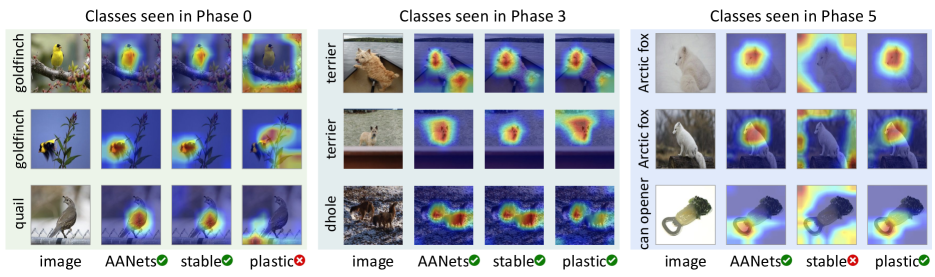
Figure 3: The activation maps using Grad-CAM [39] for the 5-th phase (the last phase) model on ImageNet-Subset ($N$=5). Samples are selected from the classes coming in the 0-th phase (left), the 3-rd phase (middle), and the 5-th phase (right), respectively. Green tick (red cross) means the discriminative features are activated on the object regions successfully (unsuccessfully). $\bar{\alpha}_{\eta}=0.428$ and $\bar{\alpha}_{\phi}=0.572$.

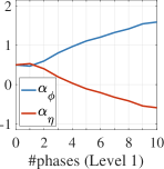
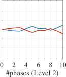
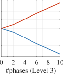
(a) CIFAR-100 ($N$=10)

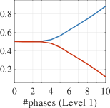
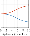
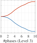
(b) ImageNet-Subset ($N$=10)

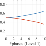
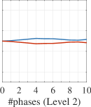
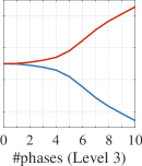
(c) ImageNet ($N$=10)

Figure 4: The values of $\alpha_{\eta}$ and $\alpha_{\phi}$ adapted for each residual level and in each incremental phase. All curves are smoothed with a rate of $0.8$ for better visualization.

Comparing to the State-of-the-Art. Table 2 shows that taking our AANets as a plug-in architecture for $4$ state-of-the-art methods [34, 16, 25, 11] consistently improves their model performances. E.g., for CIFAR-100, LUCIR w/ AANets and Mnemonics w/ AANets respectively gains $4.9\%$ and $3.3\%$ improvements on average. From Table 2, we can see that our approach of using AANets achieves top performances in all settings. Interestingly, we find that AANets can boost more performance for simpler baseline methods, e.g., iCaRL. iCaRL w/ AANets achieves mostly better results than those of LUCIR on three datasets, even though the latter method deploys various regularization techniques.

Visualizing Activation Maps. Figure 3 demonstrates the activation maps visualized by Grad-CAM for the final model (obtained after $5$ phases) on ImageNet-Subset ($N$=5). The visualized samples from left to right are picked from the classes coming in the $0$-th, $3$-rd and $5$-th phases, respectively. For the $0$-th phase samples, the model makes the prediction according to foreground regions (right) detected by the stable block and background regions (wrong) by the plastic block. This is because, through multiple phases of full updates, the plastic block forgets the knowledge of these old samples while the stable block successfully retains it. This situation is reversed when using that model to recognize the $5$-th phase samples. The reason is that the stable block is far less learnable than the plastic block, and may fail to adapt to new data. For all shown samples, the model extracts features as informative as possible in two blocks. Then, it aggregates these features using the weights adapted from the balanced dataset, and thus can make a good balance of the features to achieve the best prediction.

Aggregation Weights ($\alpha_{\eta}$ and $\alpha_{\phi}$). Figure 4 shows the values of $\alpha_{\eta}$ and $\alpha_{\phi}$ learned during training $10$-phase models. Each row displays three plots for three residual levels of AANets respectively. Comparing among columns, we can see that Level 1 tends to get larger values of $\alpha_{\phi}$, while Level 3 tends to get larger values of $\alpha_{\eta}$. This can be interpreted as lower-level residual blocks learn to stay stabler which is intuitively correct in deep models. With respect to the learning activity of CIL models, it is to continuously transfer the learned knowledge to subsequent phases. The features at different resolutions (levels in our case) have different transferabilities [50]. Level 1 encodes low-level features that are more stable and shareable among all classes. Level 3 nears the classifiers, and tends to be more plastic such as to fast to adapt to new classes.

5 Conclusions

We introduce a novel network architecture AANets specially for CIL. Our main contribution lies in addressing the issue of stability-plasticity dilemma in CIL by a simple modification on plain ResNets — applying two types of residual blocks to respectively and specifically learn stability and plasticity at each residual level, and then aggregating them as a final representation. To achieve efficient aggregation, we adapt the level-specific and phase-specific weights in an end-to-end manner. Our overall approach is generic and can be easily incorporated into existing CIL methods to boost their performance.

Acknowledgments. This research is supported by A*STAR under its AME YIRG Grant (Project No. A20E6c0101), the Singapore Ministry of Education (MOE) Academic Research Fund (AcRF) Tier 1, Alibaba Innovative Research (AIR) programme, Major Scientific Research Project of Zhejiang Lab (No. 2019DB0ZX01), and Max Planck Institute for Informatics.

Supplementary Materials

These supplementary materials include the results for different CIL settings(§A), “strict memory budget” experiments (§B), additional ablation results (§C), additional plots (§D), more visualization results (§E), and the execution steps of our source code with PyTorch (§F).

A Results for Different CIL Settings.

We provide more results on the setting with the same number of classes at all phases [32] in the second block (“same # of cls”) of Table S1. For example, $N$=$25$ indicates $100$ classes evenly come in $25$ phases, so $4$ new classes arrive in each phase (including the $0$-th phase). Further, in this table, each entry represents an accuracy of the last phase (since all-phase accuracies are not comparable to our original setting) averaged over $3$ runs; and “update $\theta_{\mathrm{base}}$” means that $\theta_{\mathrm{base}}$ is updated as $\theta_{\mathrm{base}}\leftarrow\phi_{i}\odot\theta_{\mathrm{base}}$ after each phase. All results are under “strict memory budget” and “all”+“scaling” settings, so $\phi_{i}$ indicate the meta-learned weights of SS operators. The results show that 1) “w/ AANets” performs best in all settings and brings consistent improvements; and 2) “update $\theta_{\mathrm{base}}$” is helpful for CIFAR-100 but harmful for ImageNet-Subset.

Last-phase acc. (%)	CIFAR-100				ImageNet-Subset
	$N$=5	10	25		5	10	25
LUCIR (50 cls in Phase 0)	54.3	50.3	48.4		60.0	57.1	49.3
w/ AANets	58.6	56.7	53.3		64.3	58.0	56.5
LUCIR (same # of cls)	52.1	44.9	40.6		60.3	52.5	53.3
w/ AANets, update $\theta{{}_{\mathrm{base}}}$	54.3	47.4	42.4		61.4	52.5	48.2
w/ AANets	52.6	46.1	41.9		68.8	60.8	56.8

Table S1: Supplementary to Table 1. Last-phase accuracies (%) for different class-incremental learning (CIL) settings.

B Strict Memory Budget Experiments

Method	CIFAR-100				ImageNet-Subset				ImageNet
	$N$=5	10	25		5	10	25		5	10	25
iCaRL [34]	57.12$\pm 0.50$	52.66$\pm 0.89$	48.22$\pm 0.76$		65.44$\pm 0.35$	59.88$\pm 0.83$	52.97$\pm 1.02$		51.50$\pm 0.43$	46.89$\pm 0.35$	43.14$\pm 0.67$
w/ AANetss (ours)	63.91$\pm 0.52$	57.65$\pm 0.81$	52.10$\pm 0.87$		71.37$\pm 0.57$	66.34$\pm 0.61$	61.87$\pm 1.01$		63.65$\pm 1.02$	61.14$\pm 0.59$	55.91$\pm 0.95$
	64.22$\pm 0.42$	60.26$\pm 0.73$	56.43$\pm 0.81$		73.45$\pm 0.51$	71.78$\pm 0.64$	69.22$\pm 0.83$		63.91$\pm 0.59$	61.28$\pm 0.49$	56.97$\pm 0.86$
LUCIR [16]	63.17$\pm 0.87$	60.14$\pm 0.73$	57.54$\pm 0.43$		70.84$\pm 0.69$	68.32$\pm 0.81$	61.44$\pm 0.91$		64.45$\pm 0.32$	61.57$\pm 0.23$	56.56$\pm 0.36$
w/ AANetss (ours)	66.46$\pm 0.45$	65.38$\pm 0.53$	61.79$\pm 0.51$		72.21$\pm 0.87$	69.10$\pm 0.90$	67.10$\pm 0.54$		64.83$\pm 0.50$	62.34$\pm 0.65$	60.49$\pm 0.78$
	66.74$\pm 0.37$	65.29$\pm 0.43$	63.50$\pm 0.61$		72.55$\pm 0.67$	69.22$\pm 0.72$	67.60$\pm 0.39$		64.94$\pm 0.25$	62.39$\pm 0.61$	60.68$\pm 0.58$
Mnemonics [25]	63.34$\pm 0.62$	62.28$\pm 0.43$	60.96$\pm 0.72$		72.58$\pm 0.85$	71.37$\pm 0.56$	69.74$\pm 0.39$		64.54$\pm 0.49$	63.01$\pm 0.57$	61.00$\pm 0.71$
w/ AANetss (ours)	66.12$\pm 0.00$	65.10$\pm 0.00$	61.83$\pm 0.00$		72.88$\pm 0.00$	71.50$\pm 0.00$	70.49$\pm 0.00$		65.21$\pm 0.76$	63.36$\pm 0.67$	61.37$\pm 0.80$
	67.59$\pm 0.34$	65.66$\pm 0.61$	63.35$\pm 0.72$		72.91$\pm 0.53$	71.93$\pm 0.37$	70.70$\pm 0.45$		65.23$\pm 0.62$	63.60$\pm 0.71$	61.53$\pm 0.29$
PODNet-CNN [11]	64.83$\pm 1.11$	63.19$\pm 1.31$	60.72$\pm 1.54$		75.54$\pm 0.29$	74.33$\pm 1.05$	68.31$\pm 2.77$		66.95	64.13	59.17
w/ AANetss (ours)	66.36$\pm 1.02$	64.31$\pm 1.13$	61.80$\pm 1.24$		76.63$\pm 0.35$	75.00$\pm 0.78$	71.43$\pm 1.51$		67.80$\pm 0.87$	64.80$\pm 0.60$	61.01$\pm 0.97$
	66.31$\pm 0.87$	64.31$\pm 0.90$	62.31$\pm 1.02$		76.96$\pm 0.53$	75.58$\pm 0.74$	71.78$\pm 0.81$		67.73$\pm 0.71$	64.85$\pm 0.53$	61.78$\pm 0.61$

Table S2: Supplementary to Table 2. Using “strict memory budget” setting. Average incremental accuracies (%) of four state-of-the-art methods w/ and w/o our AANetss as a plug-in architecture. The red lines are the corresponding results in Table 2 of the main paper.

In Table S2, we present the results of $4$ state-of-the-art methods w/ and w/o AANetss as a plug-in architecture, under the “strict memory budget” setting which strictly controls the total memory shared by the exemplars and the model parameters. For example, if we incorporate AANetss to LUCIR [16], we need to reduce the number of exemplars to balance the additional memory introduced by AANetss (as AANetss take around $20\%$ more parameters than the plain ResNets used in LUCIR [16]). As a result, we reduce the numbers of exemplars for AANetss from $20$ to $13$, $16$ and $19$, respectively, for CIFAR-100, ImageNet-Subset, and ImageNet, in the “strict memory budget” setting. For CIFAR-100, we use $530k$ additional parameters, so we need to reduce $530k\mathrm{floats}\times 4\mathrm{bytes/float}\div(32\times 32\times 3\mathrm{bytes}/\mathrm{image})\div 100\mathrm{classes}\approx 6.9\mathrm{images}/\mathrm{class}$, and $\lceil 6.9\rceil=7\mathrm{images}/\mathrm{class}$. For ImageNet-Subset, we use $12.6M$ additional parameters, so we need to reduce $12.6M\mathrm{floats}\times 4\mathrm{bytes/float}\div(224\times 224\times 3\mathrm{bytes}/\mathrm{image})\div 100\mathrm{classes}\approx 3.3\mathrm{images}/\mathrm{class}$, and $\lceil 3.3\rceil=4\mathrm{images}/\mathrm{class}$. For ImageNet, we use $12.6M$ additional parameters, so we need to reduce $12.6M\mathrm{floats}\times 4\mathrm{bytes/float}\div(224\times 224\times 3\mathrm{bytes}/\mathrm{image})\div 100\mathrm{classes}\approx 0.3\mathrm{images}/\mathrm{class}$, and $\lceil 0.3\rceil=1\mathrm{image}/\mathrm{class}$. From Table S2, we can see that our approach of using AANetss still achieves the top performances in all CIL settings even if the “strict memory budget” is applied.

C More Ablation Results

Row		Ablation Setting				CIFAR-100 (acc.%)							ImageNet-Subset (acc.%)
						Memory	FLOPs	#Param	$N$=5	10	25		Memory	FLOPs	#Param	$N$=5	10	25
1	single-branch “all” [16]					7.64MB	70M	469K	63.17	60.14	57.54		330MB	1.82G	11.2M	70.84	68.32	61.44
2	“all” + “all”					9.43MB	140M	938K	64.49	61.89	58.87		372MB	3.64G	22.4M	69.72	66.69	63.29
3	$4\times$ “all”					13.01MB	280M	1.9M	65.13	64.08	59.40		456MB	7.28G	44.8M	70.12	67.31	64.00
4	single-branch “scaling”					7.64MB	70M	60K	62.48	61.53	60.17		334MB	1.82G	1.4M	71.29	68.88	66.75
5	“scaling” + “scaling”					9.43MB	140M	120K	65.13	64.08	62.50		382MB	3.64G	2.8M	71.71	71.07	66.69
6	$4\times$ “scaling”					13.01MB	240M	280K	66.00	64.67	63.16		478MB	3.64G	5.6M	72.01	71.23	67.12
7	“all” + “scaling”					9.66MB	140M	530K	66.74	65.29	63.50		378MB	3.64G	12.6M	72.55	69.22	67.60
8	“all” + “frozen”					9.43MB	140M	469K	65.62	64.05	63.67		372MB	3.64G	11.2M	71.71	69.87	67.92
9	“scaling” + “frozen”					9.66MB	140M	60K	64.71	63.65	62.89		378MB	3.64G	1.4M	73.01	71.65	70.30

Table S3: Supplementary to Table 1. More ablation study. “$4\times$” denotes that we use $4$ same-type blocks at each residual level.

In Table S3, we supplement the ablation results obtained in more settings. “$4\times$” denotes that we use $4$ same-type blocks at each residual level. Comparing Row 7 to Row 2 (Row 5) shows the efficiency of using different types of blocks for representing stability and plasticity.

D Additional Plots

In Figures S2, we present the phase-wise accuracies obtained on CIFAR-100, ImageNet-Subset and ImageNet, respectively. “Upper Bound” shows the results of joint training with all previous data accessible in every phase. We can observe that our method achieves the highest accuracies in almost every phase of different settings. In Figures S3 and S4, we supplement the plots for the values of $\alpha_{\eta}$ and $\alpha_{\phi}$ learned on the CIFAR-100 and ImageNet-Subset ($N$=$5$, $25$). All curves are smoothed with a rate of $0.8$ for a better visualization.

E More Visualization Results

Figure S1 below shows the activation maps of a “goldfinch” sample (seen in Phase 0) in different-phase models (ImageNet-Subset, $N$=$5$). Notice that the plastic block gradually loses its attention on this sample (i.e., forgets it), while the stable block retains it. AANets benefit from its stable blocks.

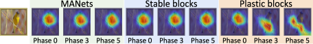
Figure S1: Supplementary to Figure 3. The activation maps of a “goldfinch” sample (seen in Phase 0) in different-phase models (ImageNet-Subset; $N$=$5$).

F Source Code in PyTorch

We provide our PyTorch code on https://class-il.mpi-inf.mpg.de/. To run this repository, we kindly advise you to install Python 3.6 and PyTorch 1.2.0 with Anaconda.

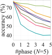
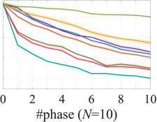
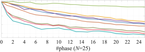
(a) CIFAR-100 ($100$ classes). In the $0$-th phase, $\theta_{\mathrm{base}}$ is trained on $50$ classes, the remaining classes are given evenly in the subsequent phases.

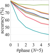
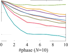
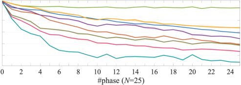
(b) ImageNet-Subset ($100$ classes). In the $0$-th phase, $\theta_{\mathrm{base}}$ is trained on $50$ classes, the remaining classes are given evenly in the subsequent phases.

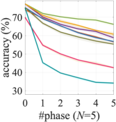
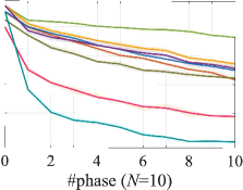
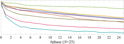
(c) ImageNet ($1000$ classes). In the $0$-th phase, $\theta_{\mathrm{base}}$ on is trained on $500$ classes, the remaining classes are given evenly in the subsequent phases.

Figure S2: Supplementary to Table 2.Phase-wise accuracies ($\%$). Light-color ribbons are visualized to show the $95\%$ confidence intervals. Comparing methods: Upper Bound (the results of joint training with all previous data accessible in each phase); PODNet (2020) [11]; Mnemonics (2020) [25]; LUCIR (2019) [16]; BiC (2019) [48]; iCaRL (2017) [34]; and LwF (2016) [23].

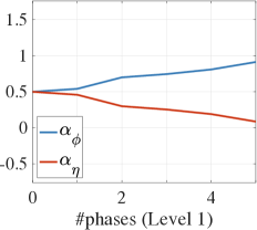
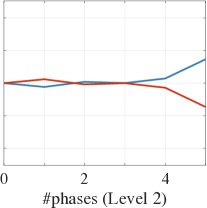
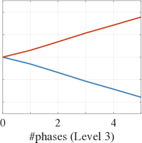
(a) CIFAR-100, $N$=5

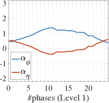
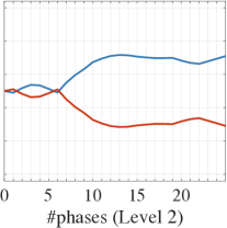
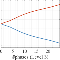
(b) CIFAR-100, $N$=25

Figure S3: Supplementary to Figure 4. The changes of values for $\alpha_{\eta}$ and $\alpha_{\phi}$ on CIFAR-100.

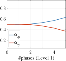
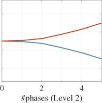
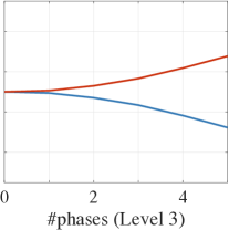
(a) ImageNet-Subset, $N$=5

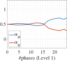
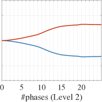
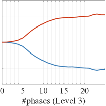
(b) ImageNet-Subset, $N$=25

Figure S4: Supplementary to Figure 4. The changes of values for $\alpha_{\eta}$ and $\alpha_{\phi}$ on ImageNet-Subset.

References

- [1] Davide Abati, Jakub Tomczak, Tijmen Blankevoort, Simone Calderara, Rita Cucchiara, and Babak Ehteshami Bejnordi. Conditional channel gated networks for task-aware continual learning. In CVPR, pages 3931–3940, 2020.
- [2] Rahaf Aljundi, Punarjay Chakravarty, and Tinne Tuytelaars. Expert gate: Lifelong learning with a network of experts. In CVPR, pages 3366–3375, 2017.
- [3] Eden Belouadah and Adrian Popescu. Il2m: Class incremental learning with dual memory. In CVPR, pages 583–592, 2019.
- [4] Francisco M. Castro, Manuel J. Marín-Jiménez, Nicolás Guil, Cordelia Schmid, and Karteek Alahari. End-to-end incremental learning. In ECCV, pages 241–257, 2018.
- [5] Arslan Chaudhry, Puneet K Dokania, Thalaiyasingam Ajanthan, and Philip HS Torr. Riemannian walk for incremental learning: Understanding forgetting and intransigence. In ECCV, pages 532–547, 2018.
- [6] Arslan Chaudhry, Marc’Aurelio Ranzato, Marcus Rohrbach, and Mohamed Elhoseiny. Efficient lifelong learning with a-gem. In ICLR, 2019.
- [7] Zhiyuan Chen and Bing Liu. Lifelong machine learning. Synthesis Lectures on Artificial Intelligence and Machine Learning, 12(3):1–207, 2018.
- [8] Guy Davidson and Michael C Mozer. Sequential mastery of multiple visual tasks: Networks naturally learn to learn and forget to forget. In CVPR, pages 9282–9293, 2020.
- [9] Matthias De Lange, Rahaf Aljundi, Marc Masana, Sarah Parisot, Xu Jia, Ales Leonardis, Gregory Slabaugh, and Tinne Tuytelaars. Continual learning: A comparative study on how to defy forgetting in classification tasks. arXiv, 1909.08383, 2019.
- [10] Matthias De Lange, Rahaf Aljundi, Marc Masana, Sarah Parisot, Xu Jia, Aleš Leonardis, Gregory Slabaugh, and Tinne Tuytelaars. A continual learning survey: Defying forgetting in classification tasks. arXiv, 1909.08383, 2019.
- [11] Arthur Douillard, Matthieu Cord, Charles Ollion, Thomas Robert, and Eduardo Valle. Podnet: Pooled outputs distillation for small-tasks incremental learning. In ECCV, 2020.
- [12] Chelsea Finn, Pieter Abbeel, and Sergey Levine. Model-agnostic meta-learning for fast adaptation of deep networks. In ICML, pages 1126–1135, 2017.
- [13] Ian Goodfellow, Jean Pouget-Abadie, Mehdi Mirza, Bing Xu, David Warde-Farley, Sherjil Ozair, Aaron Courville, and Yoshua Bengio. Generative adversarial nets. In NIPS, pages 2672–2680, 2014.
- [14] Kaiming He, Xiangyu Zhang, Shaoqing Ren, and Jian Sun. Deep residual learning for image recognition. In CVPR, pages 770–778, 2016.
- [15] Geoffrey E. Hinton, Oriol Vinyals, and Jeffrey Dean. Distilling the knowledge in a neural network. arXiv, 1503.02531, 2015.
- [16] Saihui Hou, Xinyu Pan, Chen Change Loy, Zilei Wang, and Dahua Lin. Learning a unified classifier incrementally via rebalancing. In CVPR, pages 831–839, 2019.
- [17] Wenpeng Hu, Zhou Lin, Bing Liu, Chongyang Tao, Zhengwei Tao, Jinwen Ma, Dongyan Zhao, and Rui Yan. Overcoming catastrophic forgetting for continual learning via model adaptation. In ICLR, 2019.
- [18] Xinting Hu, Kaihua Tang, Chunyan Miao, Xian-Sheng Hua, and Hanwang Zhang. Distilling causal effect of data in class-incremental learning. In CVPR, 2021.
- [19] Ronald Kemker, Marc McClure, Angelina Abitino, Tyler L. Hayes, and Christopher Kanan. Measuring catastrophic forgetting in neural networks. In AAAI, pages 3390–3398, 2018.
- [20] Alex Krizhevsky, Geoffrey Hinton, et al. Learning multiple layers of features from tiny images. Technical report, Citeseer, 2009.
- [21] Xinzhe Li, Qianru Sun, Yaoyao Liu, Qin Zhou, Shibao Zheng, Tat-Seng Chua, and Bernt Schiele. Learning to self-train for semi-supervised few-shot classification. In NeurIPS, pages 10276–10286, 2019.
- [22] Yingying Li, Xin Chen, and Na Li. Online optimal control with linear dynamics and predictions: Algorithms and regret analysis. In NeurIPS, pages 14858–14870, 2019.
- [23] Zhizhong Li and Derek Hoiem. Learning without forgetting. IEEE Transactions on Pattern Analysis and Machine Intelligence, 40(12):2935–2947, 2018.
- [24] Yaoyao Liu, Bernt Schiele, and Qianru Sun. An ensemble of epoch-wise empirical bayes for few-shot learning. In ECCV, pages 404–421, 2020.
- [25] Yaoyao Liu, Yuting Su, An-An Liu, Bernt Schiele, and Qianru Sun. Mnemonics training: Multi-class incremental learning without forgetting. In CVPR, pages 12245–12254, 2020.
- [26] David Lopez-Paz and Marc’Aurelio Ranzato. Gradient episodic memory for continual learning. In NIPS, pages 6467–6476, 2017.
- [27] Michael McCloskey and Neal J Cohen. Catastrophic interference in connectionist networks: The sequential learning problem. In Psychology of Learning and Motivation, volume 24, pages 109–165. Elsevier, 1989.
- [28] K. McRae and P. Hetherington. Catastrophic interference is eliminated in pre-trained networks. In CogSci, 1993.
- [29] Martial Mermillod, Aurélia Bugaiska, and Patrick Bonin. The stability-plasticity dilemma: Investigating the continuum from catastrophic forgetting to age-limited learning effects. Frontiers in Psychology, 4:504, 2013.
- [30] Ameya Prabhu, Philip HS Torr, and Puneet K Dokania. Gdumb: A simple approach that questions our progress in continual learning. In ECCV, 2020.
- [31] Jathushan Rajasegaran, Munawar Hayat, Salman H Khan, Fahad Shahbaz Khan, and Ling Shao. Random path selection for continual learning. In NeurIPS, pages 12669–12679, 2019.
- [32] Jathushan Rajasegaran, Salman Khan, Munawar Hayat, Fahad Shahbaz Khan, and Mubarak Shah. itaml: An incremental task-agnostic meta-learning approach. In CVPR, pages 13588–13597, 2020.
- [33] R. Ratcliff. Connectionist models of recognition memory: Constraints imposed by learning and forgetting functions. Psychological Review, 97:285–308, 1990.
- [34] Sylvestre-Alvise Rebuffi, Alexander Kolesnikov, Georg Sperl, and Christoph H Lampert. iCaRL: Incremental classifier and representation learning. In CVPR, pages 5533–5542, 2017.
- [35] Matthew Riemer, Ignacio Cases, Robert Ajemian, Miao Liu, Irina Rish, Yuhai Tu, and Gerald Tesauro. Learning to learn without forgetting by maximizing transfer and minimizing interference. In ICLR, 2019.
- [36] Matthew Riemer, Ignacio Cases, Robert Ajemian, Miao Liu, Irina Rish, Yuhai Tu, and Gerald Tesauro. Learning to learn without forgetting by maximizing transfer and minimizing interference. In ICLR, 2019.
- [37] Olga Russakovsky, Jia Deng, Hao Su, Jonathan Krause, Sanjeev Satheesh, Sean Ma, Zhiheng Huang, Andrej Karpathy, Aditya Khosla, Michael Bernstein, et al. Imagenet large scale visual recognition challenge. International Journal of Computer Vision, 115(3):211–252, 2015.
- [38] Andrei A Rusu, Neil C Rabinowitz, Guillaume Desjardins, Hubert Soyer, James Kirkpatrick, Koray Kavukcuoglu, Razvan Pascanu, and Raia Hadsell. Progressive neural networks. arXiv, 1606.04671, 2016.
- [39] Ramprasaath R Selvaraju, Michael Cogswell, Abhishek Das, Ramakrishna Vedantam, Devi Parikh, and Dhruv Batra. Grad-cam: Visual explanations from deep networks via gradient-based localization. In CVPR, pages 618–626, 2017.
- [40] Hanul Shin, Jung Kwon Lee, Jaehong Kim, and Jiwon Kim. Continual learning with deep generative replay. In NIPS, pages 2990–2999, 2017.
- [41] Ankur Sinha, Pekka Malo, and Kalyanmoy Deb. A review on bilevel optimization: From classical to evolutionary approaches and applications. IEEE Transactions on Evolutionary Computation, 22(2):276–295, 2018.
- [42] Qianru Sun, Yaoyao Liu, Zhaozheng Chen, Tat-Seng Chua, and Bernt Schiele. Meta-transfer learning through hard tasks. IEEE Transactions on Pattern Analysis and Machine Intelligence, 2020.
- [43] Qianru Sun, Yaoyao Liu, Tat-Seng Chua, and Bernt Schiele. Meta-transfer learning for few-shot learning. In CVPR, pages 403–412, 2019.
- [44] Xiaoyu Tao, Xinyuan Chang, Xiaopeng Hong, Xing Wei, and Yihong Gong. Topology-preserving class-incremental learning. In ECCV, 2020.
- [45] Heinrich Von Stackelberg and Stackelberg Heinrich Von. The theory of the market economy. Oxford University Press, 1952.
- [46] Tongzhou Wang, Jun-Yan Zhu, Antonio Torralba, and Alexei A. Efros. Dataset distillation. arXiv, 1811.10959, 2018.
- [47] Max Welling. Herding dynamical weights to learn. In ICML, pages 1121–1128, 2009.
- [48] Yue Wu, Yinpeng Chen, Lijuan Wang, Yuancheng Ye, Zicheng Liu, Yandong Guo, and Yun Fu. Large scale incremental learning. In CVPR, pages 374–382, 2019.
- [49] Ju Xu and Zhanxing Zhu. Reinforced continual learning. In NeurIPS, pages 899–908, 2018.
- [50] Jason Yosinski, Jeff Clune, Yoshua Bengio, and Hod Lipson. How transferable are features in deep neural networks? In NIPS, pages 3320–3328, 2014.
- [51] Lu Yu, Bartlomiej Twardowski, Xialei Liu, Luis Herranz, Kai Wang, Yongmei Cheng, Shangling Jui, and Joost van de Weijer. Semantic drift compensation for class-incremental learning. In CVPR, pages 6982–6991, 2020.
- [52] Chi Zhang, Yujun Cai, Guosheng Lin, and Chunhua Shen. Deepemd: Few-shot image classification with differentiable earth mover’s distance and structured classifiers. In CVPR, pages 12203–12213, 2020.
- [53] Chi Zhang, Nan Song, Guosheng Lin, Yun Zheng, Pan Pan, and Yinghui Xu. Few-shot incremental learning with continually evolved classifiers. In CVPR, 2021.
- [54] Bowen Zhao, Xi Xiao, Guojun Gan, Bin Zhang, and Shu-Tao Xia. Maintaining discrimination and fairness in class incremental learning. In CVPR, pages 13208–13217, 2020.