Valid $t$-ratio Inference for IV

David S. Lee
Princeton University and NBER

Justin McCrary
Columbia University and NBER

Marcelo J. Moreira
FGV EPGE

Jack Porter
University of Wisconsin

March 10, 2024

In the single IV model, current practice relies on the first-stage $F$ exceeding some threshold (e.g., 10) as a criterion for trusting $t$-ratio inferences, even though this yields an anti-conservative test. We show that a true 5 percent test instead requires an $F$ greater than 104.7. Maintaining 10 as a threshold requires replacing the critical value 1.96 with 3.43. We re-examine 57 AER papers and find that corrected inference causes half of the initially presumed statistically significant results to be insignificant. We introduce a more powerful test, the $tF$ procedure, which provides $F$-dependent adjusted $t$-ratio critical values.

Keywords: Instrumental Variables, Weak Instruments, $t$-ratio, First-stage $F$ statistic

1 Introduction

Consider the single-variable instrumental variable (IV) model, with outcome $Y$, regressor of interest $X$, and instrument $Z$,

$$Y=\alpha+\beta X+u\text{, where}$$ (1)

$$COV\left(u,Z\right)=0\text{.}$$

When describing statistical inference procedures for these models, textbooks invariably recommend estimating $\beta$ via the instrumental variable estimator $\hat{\beta}_{IV}\equiv\frac{\hat{COV}\left(Y,Z\right)}{\hat{COV}\left(X,Z\right)}$ and associated standard error $\hat{SE}\left(\hat{\beta}_{IV}\right)$ and testing the null hypothesis that $\beta=\beta_{0}$ using the $t$-ratio $\frac{\hat{\beta}_{IV}-\beta_{0}}{\hat{SE}\left(\hat{\beta}_{IV}\right)}$ with the usual critical value of $1.96$ for a test at the 5 percent level of significance, or constructing 95 percent confidence intervals using the interval $\hat{\beta}_{IV}\pm 1.96\cdot\hat{SE}\left(\hat{\beta}_{IV}\right)$. Most textbook treatments also note that these inference procedures give distorted Type I error (or coverage rates) when instruments are “weak,” and suggest using the first-stage $F$ statistic as a diagnostic, implying that one can reliably use the usual procedures if $F$ exceeds a threshold, such as 10.

Even though these $t$-ratio inference procedures are known to yield distortions in size and coverage rates, and even though alternatives (e.g., AndersonRubin49) are known to have correct size/coverage – possessing attractive optimality properties while also being robust to arbitrarily weak instruments – applied research, with rare exceptions, relies on $t$-ratio-based inference. This continued practice is arguably based on a combination of a preference for analytical and computational convenience and the presumption that for practical purposes, the distortions in inference are small or negligible.

This paper theoretically and empirically assesses this presumption. Specifically, we derive expressions for the rejection probabilities for both the conventional $t$-ratio procedure and the common procedure of using a threshold for the first-stage $F$ statistic to account for weak instruments. We use these expressions to precisely answer the following sets of questions: 1) Since it is known that being completely agnostic about the data-generating process will lead to $t$-ratio-based inference that will deliver incorrect size and confidence level (e.g., because of weak instruments), precisely which additional assumptions about the model in (1) can be imposed so that the conventional $t$-ratio procedure is valid? and 2) Since it is known that using the usual $t$-ratio procedure in conjunction with a modest threshold rule for $F$ (e.g., 10) will yield Type I error that is too large, is there a threshold for $F$ (or, alternatively, a higher critical value for $t$) that would yield inferences with the intended size and confidence level? In other words, since it would be inaccurate to refer to these procedures as having the intended 5 percent Type I error, are there adjustments that can be made that would result in a true 5 percent test?

Our answers to these questions indicate that fixing these distortions (or specifying the assumptions needed to avoid the distortions) leads to a significant change to interpretation and practice. The IV $t$-ratio procedure is typically presented as asymptotically valid, applicable without needing to make any assumptions about model (1), other than $COV\left(X,Z\right)\neq 0$. But the results of Dufour97 show that the $t$-ratio procedure will lead to incorrect coverage in any (arbitrarily large) finite sample. We quantify this distortion, by showing that the usual $1.96$ critical values for a 5 percent test can remain valid if one assumes that $E\left[F\right]$ exceeds 143; strictly speaking, our calculations show that there exist data-generating processes with $E\left[F\right]<$ 143 that could lead to rejection probabilities (coverage probabilities) greater than 0.05 (less than 0.95). Without knowing the true value of the nuisance parameter $E\left[F\right]$, the rejection probability can be arbitrarily close to 1.

We also show that an alternative assumption can be used to justify the validity of the usual $t$-ratio procedure. This alternative assumption is agnostic about $E\left[F\right]$ but instead limits the degree of endogeneity. Namely, it requires the correlation between the main equation and first-stage errors, $\rho\equiv Corr\left(u,X-Z\pi\right)$, be no greater than 0.565 in absolute value. Again, allowing the possibility of $\left|\rho\right|$ being greater than $0.565$ could potentially lead to the maximum distortion in type I error possible (e.g., rejecting with probability 1). These potential restrictions on $E[F]$ or $|\rho|$ appear to be significant departures from agnosticism about nuisance parameters.

Examining the more standard case, in which practitioners wish to remain agnostic about $E\left[F\right]$ and $\rho$, we find that substantial changes to common usage of the first-stage $F$ are required for inferences to be undistorted. As noted above, perhaps the most commonly employed rule of thumb for the first-stage $F$ statistic is a threshold of $10$: if $F$ is beyond 10, then the usual critical values of $1.96$ are typically used, with the understanding that there is a “small” amount of distortion to size/coverage. We show that it is in fact possible to adjust the threshold for $F$ to be a finite value so that there is no distortion. However, these calculations show that the distortion-corrected threshold for $F$ is far from 10, and is, in fact, 104.7.

An alternative approach is to maintain the commonly used threshold for $F$ of 10, but then to adjust the critical values for $t$ to achieve correct size and confidence level. Our calculations show that the required critical value in this case would be very large: $3.43$. To put this adjusted critical value in perspective, consider the move from a 95 percent confidence interval to a 99 percent confidence interval—an exacting standard. This move only requires adjusting the critical value by about 31 percent, i.e., from 1.96 to 2.57. Our results show that using a threshold of 10 for $F$ requires adjusting the critical value by about 74 percent, i.e., from 1.96 to 3.43, for the $t$-test to have correct size/coverage. In other words, using 3.43 as a critical value for $t$-ratio-based inference is even more stringent than using a 1 percent test and in fact is the critical value for a 0.06 percent test.

An important fact that has been recognized in the econometrics literature but possibly under-appreciated in applied research is that the validity of a decision rule that uses a single critical value for $t$ and a single threshold for $F$ requires the commitment to automatically accept the null hypothesis – no matter the realized value of $t$ – if $F$ does not exceed the threshold (e.g., $10$ or 104.7). This amounts to confidence intervals that are dependent on $F$: If $F>104.7$ (or 10), then use $\hat{\beta}_{IV}\pm 1.96\cdot\hat{SE}\left(\hat{\beta}\right)$ (or $\hat{\beta}_{IV}\pm 3.43\cdot\hat{SE}\left(\hat{\beta}\right)$); otherwise, the confidence interval for $\beta$ is the entire real line.

We consider the practical implications of these findings for applied research by examining all studies recently published in the American Economic Review ($AER$) that utilize a single-instrument specification. All of these papers use the usual $t$-ratio-based 2SLS inference outlined above, but only 2-3 percent of the specifications report the test of AndersonRubin49, despite the clear implication from the econometrics literature that this test should be part of best applied econometric practice. Surprisingly, for more than a quarter of the specifications, one cannot infer the associated first-stage $F$ statistic from the published tables. For this group of specifications, their conclusions about statistical significance at the 5 percent level could remain unaltered were they to use our results and qualify their analysis by making one of the above two assumptions about the nuisance parameters: either $E\left[F\right]>142.6$ or $\left|\rho\right|<0.565$.

For the $AER$ specifications for which an $F$ statistic can be derived from the published tables, the median is 42.0, with 25th and 75th percentiles at 12.4 and 299.5, respectively. 58 percent of the specifications satisfy both $F>10$ and the rejection rule $\left|t\right|>1.96$, which is conventionally used to determine “statistical significance.” While StaigerStock97 notes the size distortion in such a procedure, conventional wisdom in the applied literature appears to treat such a procedure as having approximately 5 percent significance level. We re-examine the specifications with $F>10$ and $t^{2}>1.96^{2}$ and find that using either of the size-corrected procedures described above to actually achieve 5 percent significance causes at least half of the specifications to become statistically insignificant, leading us to conclude that these calculations are of real importance for the field and that “$F$>10” is not a reliable rule for practical use if authors want to maintain a significance level of 5 percent.

As AndrewsStockSun19 have noted, an important limitation to adopting a single threshold for $F$ is the loss of informativeness of the data when the first-stage $F$ is below the threshold. Even more worrisome is the possibility that researchers may selectively drop the specification because the $F$ does not meet the threshold, a decision which, in repeated samples, distorts the size of the procedure even further, as those authors note. Therefore, to accommodate occurrences of $F$ that are below $104.7$, we use our theoretical results to construct a function $c\left(F\right)$ and a procedure – which we call “$tF$” – such that under the null hypothesis, $\Pr\left[t^{2}>c\left(F\right)\right]\leq 0.05$, under any values of the nuisance parameters $E\left[F\right]$ and $\rho$. Another motivation for providing this $tF$ procedure is to aid in interpreting the potentially hundreds of studies that have already been published that did not use procedures with correct size, such as $AR$. Given the prohibitive cost of re-analyzing those studies, the $tF$ procedure allows one to use already-published $t$ and $F$ statistics to reinterpret the results, conducting valid inference.

In contrast to the two “single critical value/threshold” procedures which suggest only half of published results are statistically significant at the conventional 5 percent level, the $tF$ procedure allows us to conclude that almost four-fifths are statistically significant.

The paper is organized as follows. Section 2 uses recent papers published in the AER to characterize current inferential practices for the single-instrument IV model; these patterns motivate our areas of emphasis in the theoretical discussion. Deferring details and the more in-depth theoretical discussion to Section LABEL:sec:Derivations-of-Results, Section 3 states the main theoretical results and illustrates the consequences of those results for the studies in our sample. Section LABEL:sec:Derivations-of-Results more formally derives the theoretical results, and Section LABEL:sec:Conclusion-and-Extensions concludes. Lastly, we should re-emphasize that the findings and results of this paper, including specific numerical thresholds, are not reliant on i.i.d. or homoskedastic errors. Departures from i.i.d. errors, such as two-way clustering or auto-correlation, are easily accommodated as long as a corresponding consistent robust variance estimator is also employed.

2 Inference for IV: Current Practice

This section documents current practice for the single instrumental variable model, as reflected by recent research published in the American Economic Review. Our sample frame consists of all AER papers published between 2013 and 2019, excluding proceedings papers and comments, yielding 757 articles, of which 124 included instrumental variable regressions. Of these 124 studies, 57 employed single instrumental variable (just-identified) regressions. Consistent with the conclusion of AndrewsStockSun19, this confirms that the just-identified case is an important and prevalent one from an applied perspective.

From these papers, we transcribed the coefficients, standard errors, and other statistics associated with each $IV$ regression specification. Each observation in our final dataset is a “specification,” where a single specification is defined as a unique combination of 1) outcome, 2) endogenous regressor, 3) instrument, and 4) combination of covariates. The dataset contains 1310 specifications from 57 studies; among those studies, the average number of specifications was 22.98, with a median of 9, with 25th and 75th percentiles of 4 and 21, respectively. Since the purpose of our dataset is to fully characterize specifications that are reported in published studies, our coverage of studies will be broader than that of AndrewsStockSun19, who compared $AR$-based and $t$-ratio-based inference, by obtaining the original microdata from the smaller subset of studies for which this was possible.

Each specification was placed into one of four categories, as shown in Table 1, according to the types of regressions for which coefficients and standard errors were reported: the coefficients and standard errors from 1) only the 2SLS, 2) the 2SLS and first-stage regression, 3) the 2SLS and the reduced-form regression of the outcome on the instrument, and 4) the 2SLS, the first stage, and the reduced form. In addition, we identified whether for each specification, the first-stage $F$ statistic was explicitly reported, as indicated by the first two columns in Table 1.

Figure 1: Table 1: Current Practice Implementing IV estimation, Published Papers from AER

\begin{overpic}[width=433.62pt,trim=50.18748pt 456.70624pt 130.48749pt 40.15pt,clip]{table1_V2.pdf}\end{overpic}

N=1310.Drawn from 56 published papers. Each observation represents a unique combination of outcome, regressor, instrument, and covariates. Unweighted proportions are in parentheses, and weighted proportions are in brackets, where the weights are proportional to the inverse of the number of specifications in the associated paper.

For each configuration, Table 1 reports the number of specifications, as well as proportions (parentheses) and weighted proportions (brackets), where the weight for each specification is the inverse of the total number of specifications reported from its study. Henceforth, unless otherwise specified, when we refer to proportions, we refer to the weighted proportions, since we wish to implicitly give each study equal weight in the summary statistics that we report.

Table 1 shows that the modal practice among all combinations is for 2SLS coefficients to be reported without explicitly reporting the first-stage $F$ statistic, representing about a quarter of the specifications. The second most common practice is to report both the 2SLS and the first-stage coefficients without reporting the $F$ statistic, but it should be clear that the $F$ statistic can be derived from squaring the ratio of the first-stage coefficient to its associated estimated standard error. The least common reporting combination was the 2SLS and the reduced form, while reporting the first-stage $F$ (3.8 percent).

In the foregoing analysis, in order to maximize the number of specifications for which we have a first-stage $F$ statistic, we first use the first-stage $F$ statistic as computed from the reported first-stage coefficients and standard errors, but whenever this is not possible we use the reported $F$ statistic.

Figure 1 displays the histogram of the $F$ statistics in our sample on a logarithmic scale. The weighted 25th percentile, median, and 75th percentiles are 12.41, 41.99, and 299.48, respectively. Thus, most of the reported first-stage $F$ statistics in these studies do pass commonly cited thresholds such as 10. More detail on these specifications is provided in Table 2a, which is a two-way frequency table for whether or not $t^{2}$ exceeds $1.96^{2}$ and whether or not $F$ exceeds 10. Overall, the table indicates that for about 58 percent of the specifications, the estimated 2SLS coefficient would be “statistically significant” under the usual practice of using a critical value of $1.96$ and would also loosely reject the hypothesis of “weak instruments.” We recognize that the null hypothesis of $\beta=0$ may not always be the hypothesis of interest across all the studies, and furthermore, in our data collection, we did not make any judgments as to the extent to which any particular regression specification was crucial for the conclusions of the article; note that in many cases, the 2SLS specification was used for a “placebo” analysis where insignificant results are consistent with the identification strategy of the paper. Below, our purpose is not to determine whether any particular study’s overall conclusions are unwarranted when using the corrections below. Instead, we are seeking to identify broad patterns across all studies to assess how much of a difference these corrected procedures would have made in the aggregate.

Figure 2: Figure 1: Distribution of First-stage F-statistics

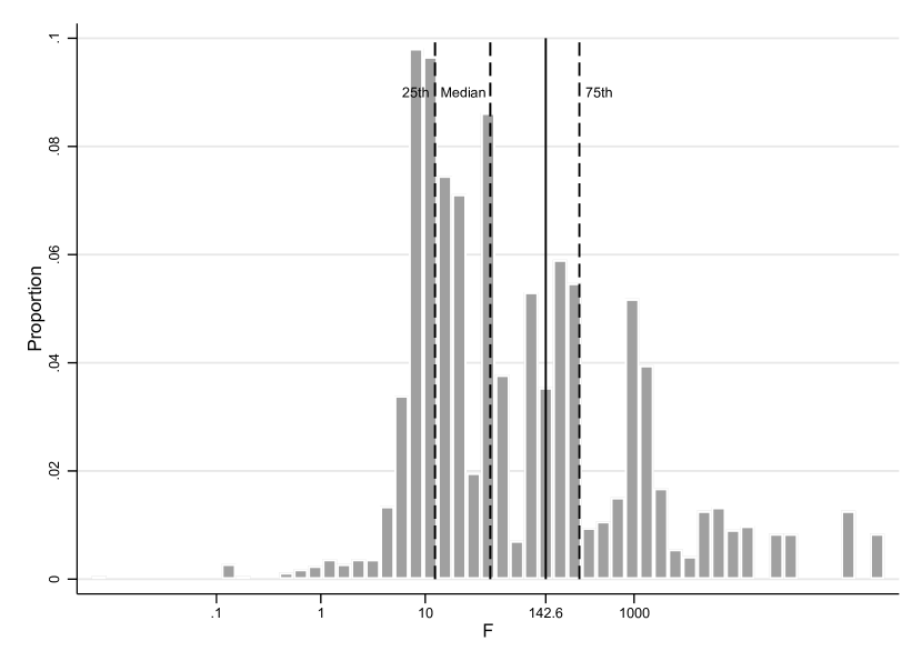
N=859 specifications. Scale is logarithmic. All specifications use the derived $F$ statistic, and when not possible, the reported $F$ statistic. Proportions are weighted; see notes to Table 1. Dashed lines correspond to the 25^th (12.41), 50^th (41.99), and 75^th (299.48) percentiles of the distribution.

Figure 3: Table 2a: $t^{2}$ and First-stage F Statistics, Conventional Critical Value, Rule of Thumb Threshold of 10

\begin{overpic}[trim=100.37498pt 582.17499pt 240.9pt 50.18748pt,clip]{table2a.pdf}\end{overpic}

N=859. Unweighted proportions are in parentheses, and weighted proportions are in brackets. See notes to Table 1.

We conclude this section with the observation that $AR$ test statistics or $AR$ confidence regions are reported for less than 3 percent of the specifications, despite the fact that the econometric literature has provided clear guidance that reporting $AR$ is part of applied econometric best practice. It is this stark difference between theory and practice that motivates our focus. We surmise that practitioners elect to use the $t$-ratio (supplemented with the use of the first-stage $F$ statistic) over the $AR$ statistic not because they believe it has superior properties, compared to $AR$-based inference, but rather because it is presumed that any inferential approximation errors associated with the conventional $t$-ratio are minimal or acceptable.

We are also motivated by the fact that there are likely hundreds of other studies that have used the single-instrument $IV$ model. Even though it can be argued that these studies should have used $AR$, if our sample is any indication, it may well be that most did not, and it could be prohibitively costly to replicate those hundreds of studies. For this reason, we take the reported statistics as given, and seek to specify precisely which assumptions previous researchers should have made to justify the inferences they made, or to reinterpret the meaning of their reported $t$ and $F$ statistics through the lens of a procedure that delivers the intended (e.g., 5 percent) level of significance.

3 Valid $t$-based Inference: Theoretical Results and Empirical Implications

This section states our main theoretical findings and defers more detailed discussion of derivations and how our findings connect to the existing econometric literature to Section LABEL:sec:Derivations-of-Results. In order to make the theory readily accessible to applied researchers, we state our findings with minimal formalism, also deferring details and nuances of the results to Section LABEL:sec:Derivations-of-Results. Whenever possible, we illustrate the practical implications of these results on the sample of studies described in Section 2. We focus on tests at the 5 percent level of significance and the corresponding 95 percent confidence interval because this is a commonly-reported standard used in applied research. However, we also report selected findings for 1 percent tests and 99 percent confidence intervals. It will be clear in Section LABEL:sec:Derivations-of-Results that our formulas can be used to analyze other levels of significance or confidence levels.

We begin by stating which restrictions on the data-generating process – over and above the textbook assumptions $COV\left(Z,u\right)=0$ and $COV\left(Z,X\right)\neq 0$ – are sufficient so that $t$-ratio-based inference procedures have approximately correct size and coverage in (arbitrarily large) finite samples. We then focus on the common practice of using the first-stage $F$ for the purposes of making inferences about $\beta$. Specifically, the results of StockYogo provide a numerical threshold (e.g., 10) for the purposes of making inferences about the strength of the instrument $Z$, defining instrument “weakness” according to the particular level of distortion – the degree of over-rejection beyond the desired Type I error. Here, we take this now-widespread notion of a single threshold for $F$ as given, and explicitly incorporate that threshold into an inference procedure on the parameter of interest $\beta$. In particular, we seek procedures that have zero distortion.

Finally, motivated by the findings below that these simple adjustments to common procedures greatly alter the width of the confidence intervals, we maintain the notion of incorporating the first-stage $F$ statistic for inference on $\beta$, and propose an extension to gain improvements in power.

3.1 Sufficient and Necessary Assumptions for Valid Inference: $t$-ratio only

As shown in Table 1, about one-quarter of the specifications reported in our sample of published AER papers do not report enough information to compute the first-stage $F$.

From Dufour97, we know that any finite critical value for the $t$-ratio will lead to over-rejection for certain values of the model’s nuisance parameters. So, we start by seeking specific restrictions on the nuisance parameters that will allow standard $t$-ratio inference to achieve correct size and confidence level. There are two key (generally unknown) nuisance parameters to consider, $E\left[F\right]$ where $F$ is the first-stage $F$-statistic, and $\rho\equiv Corr\left(u,v\right)$ where $u\equiv y-\alpha-x\beta$ and $v\equiv X-Z\pi$.

Next we explore precisely what restrictions would be sufficient or necessary so that using the usual critical value of $1.96$ would result in correct size (and coverage rates for confidence intervals). To gain some intuition for potential restrictions on $E\left[F\right]$, note that when instruments are weak (corresponding to small values of $E\left[F\right]$), the size of a conventional $t$-test with critical value 1.96 can be arbitrarily close to one. On the other hand, when the instruments are especially strong (large values of $E\left[F\right]$), the size of the conventional $t$-test with critical value 1.96 will be arbitrarily close to its nominal size of 5 percent. Perhaps surprisingly, the change in the size of the conventional $t$-test with critical value 1.96 as we move from weak to strong instruments is not monotonically decreasing, which leads to the following characterization.

Result 1a: In addition to the IV model in (1), consider the restriction that $E\left[F\right]\geq\bar{F}$. The smallest value of $\bar{F}$ such that $\Pr\left[t^{2}>1.96^{2}\right]\leq.05$ is 142.6 .

This means that in the absence of the first-stage $F$ statistic, if researchers wish to claim that their use of the $t$-ratio or confidence intervals using $1.96\cdot SE\left(\hat{\beta}_{IV}\right)$ delivers correct size and coverage, they could assume (without evidence) that the true mean of $F$ from their data is greater than 142.6. The flip side of this statement is that if the truth is that $E\left[F\right]<142.6,$ there is potential to reject the null at a rate higher than the desired nominal rate. In the extreme, the probability of rejection can be arbitrarily close to 1.

As shown in Figure 1, of the specifications for which the $F$ statistic is available, most are below 142.6, which indicates that it might be tenuous to assume $E[F]>142.6$ for those studies that do not report the first-stage $F$. At a minimum, there is every indication that such an assumption could be quite restrictive in practice.

Next we consider restrictions on the other key nuisance parameter, $\rho$. The following result presents an alternative to Result 1a, but focused on $\rho$ instead of $E[F]$.

Result 1b: In addition to the IV model in (1), consider the restriction that $\left|\rho\right|<\bar{\rho}$. The largest value of $\bar{\rho}$ such that $\Pr\left[t^{2}>1.96^{2}\right]\leq.05$ is 0.565.

In words, Result 1b says that if a researcher is willing to assume that the degree of endogeneity is not too large, one can remain agnostic about $E\left[F\right]$ (and even allow for non-identification, i.e., $E\left[F\right]=1$), and still correctly make the claim that the usual $t$-ratio procedure under the null hypothesis rejects no more than 5 percent of the time.

Remark. The above conditions are sufficient for valid inference, and they are conditions based on constant thresholds. However, in principle there are combinations of $\rho,E\left[F\right]$ under which $\Pr\left[t^{2}>1.96^{2}\right]\leq.05$, even if either one of the nuisance parameters does not fulfill the restrictions in Results 1a or 1b. The full set of combinations of values is depicted in Figure 2a; this figure is constructed using the derivations described in Section LABEL:sec:Derivations-of-Results. If the $t$-ratio procedure were valid, the entire region would be shaded. Hence, the figure illustrates in a precise way the inferential limitations of the conventional $t$-ratio alone: applied researchers may well consider assumptions about $\rho$ or $E\left[F\right]$ to be unpalatable, perhaps undermining the original appeal of the instrumental variable strategy (which is typically intended to allow one to be agnostic about $\rho$) in the first place. Figure 2a also shows immediately why hard threshold rules such as $E[F]>142.6$ or $|\rho|<0.565$ work to restore size/coverage in the IV model in (1). That is, all of the region to the left of the vertical line superimposed at $|\rho|=0.565$ is shaded, and all of the region above the horizontal line superimposed at $E[F]=142.6$ is shaded.

Figure 4: Figure 2a: Combinations of $E[F]$, $\rho$ for $Pr[t^{2}>1.96^{2}]\leq 0.05$

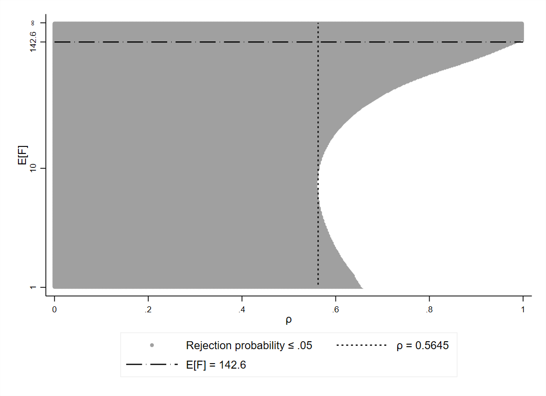
Vertical axis scale uses the transformation $\frac{\frac{E[F]}{10}}{1+\frac{E[F]}{10}}$. Shaded region represents all combinations of $E[F]$ and $\rho$ such that the rejection probability is less than or equal to 0.05. Dashed line is the maximum $\rho$ such that the region to the left is shaded. Horizontal dashed line (at 142.6) is the minimum $E[F]$ such that the region above is shaded. The rejection probabilities for $\rho<0$ mirror those for $\rho>0$.

In light of these results that show over-rejection for a nontrivial region of the nuisance parameter space, it is tempting to conclude that a simple and practical approach to avoiding these problems is to adopt a “higher standard” of statistical significance. That is, one could use the procedure with the conventional 1 percent level critical value $2.58$, and confidence intervals based on $\pm 2.58\cdot\hat{SE}\left(\hat{\beta}_{IV}\right)$. The next result shows that this approach does not, in fact, solve the size/coverage distortions discussed above. Moreover, a restriction of the parameter space for $E[F]$ no longer works at the 1 percent level.

Result 1c: For the 1 percent level of significance, there exists no $\bar{F}$ such that $\Pr\left[t^{2}>2.58^{2}\right]\leq 0.01$ for all $E\left[F\right]\geq\bar{F}$, and the largest $\bar{\rho}$ such that $\Pr\left[t^{2}>2.58^{2}\right]\leq 0.01$ for all $\left|\rho\right|\leq\bar{\rho}$ is 0.43. The full set of values of $\left|\rho\right|,E\left[F\right]$ for which $\Pr\left[t^{2}>2.58^{2}\right]\leq 0.01$ is illustrated in Figure 2b.

In Figure 2b, the shaded region is entirely contained within that of Figure 2a, indicating that the adoption of the 1 percent significance level requires stronger assumptions about the nuisance parameters for valid inference. In this sense, applied researchers should consider the use of the conventional critical values to be even more dubious at the 1 percent than at the 5 percent level.

Figure 5: Figure 2b: Combinations of $E[F]$, $\rho$ for $Pr[t^{2}>2.58^{2}]\leq 0.01$

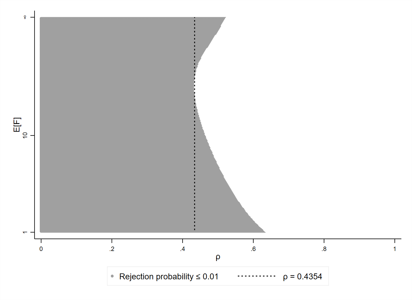
Vertical axis scale uses the transformation $\frac{\frac{E[F]}{10}}{1+\frac{E[F]}{10}}$. Shaded region represents all combinations of $E[F],\rho$ such that the rejection probability is less than or equal to 0.01. Dashed line is the maximum $\rho$ such that the region to the left is shaded.