The Color of Habitability
Abstract
From life on other planets to virtual classrooms this thesis spans a wide array of research topics all based on how we see other worlds. Our understanding of everything from moon phases, the planets in our Solar System, and exoplanet atmospheres come from our interpretation of light and one day, our knowledge of light will be used as evidence for the discovery of life on another planet.
In the time before we scattered rovers, landers, and brave souls across the Solar System we only knew of the planets and moons from the light they reflected from the Sun back to us. We are in much the same situation with exoplanets today. Our telescopes can gather the light from distant worlds but they are too far out of reach to confirm our observations with in-situ measurements. Soon we will be able to gather light from even smaller exoplanets and eventually Earth-sized exoplanets orbiting in their star’s habitable zone. As a reference guide to these upcoming observations what better place to compare to than our own Solar System. What we’ve done is take measurements of planets in our own Solar System and treat them as exoplanets to determine how different surface types can be differentiated. The result is a database of the spectra, geometric albedos, and color of 19 Solar System objects for use as an exoplanetary field guide.
A step beyond the field guide is a way to explore worlds only physics and our imaginations are limited by. By using computer models, we can create thousands of planets to determine the physical and chemical stability of any environment. One parameter domain of interest is the role of surface color on a planet’s habitability. Different materials have unique thermal properties that either cool or heat a surface depending on their color and the light that hits them. Dark oceans absorb light well and heat up while white sand is highly reflective and keeps cool. Stars emit different types of light depending on their temperature, cool stars are red while hot stars are blue. Blue starlight on a blue surface will stay cool while blue light on a red surface will heat up and vice-versa for red starlight. This results in a complicated relationship for exoplanets and stars that is important to understand if we are to properly plan observations, analyze data, and make predictions with their results.
The near future is bright for exoplanet science and as new observations dramatically change our understanding of celestial bodies so too do our methods of communicating that science. At the same time the first exoplanets were being discovered, NASA was developing the use of virtual reality to train astronauts and drive rovers on Mars. Virtual reality (VR) has come a long way since then and immersive VR headsets are now used by a fast growing audience for video games, entertainment, and education. As VR education begins to grow, we need a good understanding of its strengths and weaknesses as a teaching tool. So far, very little is know about how employing VR compares to traditional methods of teaching. By designing a learning activity on Moon phases in VR, we were able to compare the learning gains of students who used the VR version with students who used a desktop simulation or a hands-on activity. This information, coupled with the demographics of the participants, allows for a detailed breakdown of who is learning best under which conditions and plan for further study into the use of VR as a teaching tool.
Cornell Department of Astronomy and Space Sciences \subjectAstrophysics August 2020 \advisorLisa Kaltenegger
©
![[Uncaptioned image]](/html/2010.05046/assets/art/MFA_d3.jpg)
Biographical Sketch
Jack Madden grew up in Beach Haven, New Jersey before moving to Princeton, New Jersey. After graduating from Princeton High School in 2010 he went to Franklin and Marshall College in Lancaster, Pennsylvania. He worked with Dr. Froney Crawford on a pulsar survey of the Small and Large Magellanic clouds and spent the summer of 2013 at Goddard Spaceflight Center working with Dr. Lynn Carter, and Dr. Catherine Neish on Lunar impact melts. He received his B. A. in astrophysics from F&M in 2014. He went on to pursue a Ph. D. in astrophysics at Cornell University in Ithaca, New York working with Dr. Lisa Kaltenegger on exoplanet habitability. After successfully defending this thesis in May of 2020, he went on to pursue an MFA at the Rhode Island School of Design.
Acknowledgments
Mom and Dad. It’s so relaxing to know your love is unconditional. Having you here for me as a given means I can calmly focus on what I love to do, without worry. I appreciate every decision you’ve made because it got me to where I am today. Everything I do, you’ve made possible.
Will, I’m so lucky to have such a supportive brother. I know you’re always there for me and your music has been perfect to write my thesis to.
Lisa, thank you. This has been an amazing experience. I don’t think I’ll ever meet a more enthusiastic and motivated scientist. You have been so generous and supportive. Together we have done some really great work and I’m proud of what we’ve accomplished.
First years: Nic Kutsop, Victoria Calafut, Avani Gowardhan, Georgios Valogianis, Daisy Leung, Michelle Vick, Sam Birch, Eldritch, and Paul Coriles
Fellow astronomers: Yury Aglyamov, Kassandra Anderson, Cristóbal Armaza, Catie Ball, Gabe Bonilla, Ligia Fonseca Coelho, Dylan Cromer, Nils Dippe, Trevor Foote, Andrew Foster, Alex Grant,Matt Hankins, Jeremy Hodis, Jason Hofgardner, Dante Iozzo, Jonathan Jackson, Ross Jennings, Abhinav Jindal, Mike Jones, Byungdoo Kim, Thea Kozakis, Michael Lam, J.T. Laune, Marika Leitner, Cody Lemarche, Jiaru Li, Zifan Lin, C.J. Llorente, Tory Lynch, Sean Marshall, Sarah Millholland, Ishan Mishra, Kelsey Moore, Emily Moser, Eamonn O’Shea, Stella Ocker, Chris O’Connor, Swati Pandita, Tyler Pauly, Riccardo Pavesi, Bo Peng, Karen Perez, Bonan Pu, Tyler Robinson, Christopher Rooney, Morgan Saidel, Carly Snell, Tristan Stone, Yubo Su, Yilu Sun, Akshay Suresh, Christian Tate, Alex Teachey, Zoe Todd, Ngoc Truong, Amit Vishwas, Nicole Wallack, Lukas Wenzl, and JJ Zanazzi
Astronomy Department: Doug, Nena, Jason Jennings, Jessica Jones, Patricia Fernandez de Castro Martinez, Mary Mulvanerton, Cheryl Neville, Dave Pawelczyk, Zoe Ponterio, Tom Shannon, Lynda Sovocool, Jill Tarbell, Bez Thomas, and Melanie Wetzel
Cornell EMS: Catherine Appleby, Evy Baer, Hannah Bukzin, Steve Davies, Jessie Dobler, Michael Downey, Jacob Eisner, Anthony Gariolo, Meg Gordon, Ed Jaffe, George Jakubson, Alex Katz, Elise Kleine, Troy Laurence, Chad Lazar, Esteban Lopez, Dan Maas, Lakshmi Mahajan, Sean McCoy, Kyle Otto, Richa Parikh, Zac Pertucci, Dillon Sumanthiran, Galen Weld, Lily Woolf, the 18s, and all the CUPD officers who kept me safe
DBER Frank Castelli, Claire Meaders, Katherine Quinn, Emily Smith, Martin Stein, Ryan Tapping, Cole Walsh, and Monica Xu
Cornell Faculty: Nic Battaglia, Rachel Bean, Don Campbell, David Chernoff, Jim Cordes, Peter Gierasch, Riccardo Giovanelli, Alex Hayes, Martha Haynes, Terry Herter, Dong Lai, Nikole Lewis, Jamie Lloyd, Richard Lovelace, Phil Nicholson, Mason Peck, Jonathon Schuldt, Michelle Smith, Gordon Stacey, Saul Teukolsky, and Kim Williams
Researchers: Shami Chatterjee, Sid Hegde, Paul Helfenstein, Robert Hurt, Jack O’Malley James, Larry Kidder, Illeana Gomez Leal, Thomas Loredo, Ryan MacDonald, Maryame El Moutamid, Valerio Poggiali, Ramses Ramirez, Julie Rathbun, Andrew Ridden-Harper, Marina Romanova, Sarah Rugheimer, Henrik Spoon, and Jake Turner
Cornell Staff: Florio Argillas, Janine Brace, Carla DeMello, Blaine Friedlander, Linda Glaser, Sara Xayarath Hernández, and all the printing services at Cornell
Faculty and staff at Franklin and Marshall: Greg Adkins, Andy de Wet, Etienne Gagnon, Roger Godin, Lynn Johnson, Ken Krebs, Christie Larochelle, Andrea Lommen, Amy Lytle, Dan Porterfield, Beth Praton, and Calvin Stubbins
Middle and high school teachers: Mr. Komada, Mr. Floor, Mr. Carson, Mr. Skalka, Mr. Kosa, Mr. Hoffman, Ms. Agrusti-Taha, Ms. Nickman, Mrs. Cody, and Mr. Mckenna
Friends: Emily Christie, Heather Croy, Zoe Fuhrman, Hilary Gorgol, Emma Handzo, Matt Klimuszka, Adina Klingman, Dan Levin, Matt Momjian, Caitlin Rose, Charlotte Roth, Jennie Anne Simson, Betsy Sweemer, Brenna Vaughn, and Klariobaldo Zavala
Family: Grandmom, Aunt Kathryn, Nanny, Pop-pop, Katie, Patrick, Thomas, Aunt Barbara, Uncle Beard, Uncle Will, Sue, Matt, Melissa, Uncle Walt, Aunt Jan, Charlie, Alicia, Walter, Uncle Robert, Aunt Nancy, and Claire
Jacob Peacock has been the most inspirational example to me of what a scientist should be. Disguised as adventure, my love of exploring the natural world grew from the footprints we left on LBI.
Mr. Anderson was more than just that one science teacher we all had who was amazing. He helped me tap into my affinity for science and direct it purposefully to projects and independent studies. Mr. Anderson reminded all of us that science could be fun, even for high school seniors, and that science has a massive impact on our lives and future.
Froney Crawford was my first research advisor and I couldn’t have asked for a better mentor. His confidence in me, generous support, and rigorous yet lighthearted approach to science drove me to enjoy research more than I ever expected. I am constantly using what I’ve learned from Froney in my science and my life.
Jonathan Lunine has shown me that there’s always time for respect. He provides all of us with a great example of how scientists have no excuse when it comes to respecting others and valuing professionalism, diversity and inclusion, communication, and mentorship.
Andrea Stevenson Won’s fascination, expertise, and encouragement enabled me to produce work I am really proud of and didn’t think I was capable of. She inspires dedication, passion, curiosity, and everyone’s best.
Natasha Holmes, it’s hard to put into words how dramatically working with Natasha has impacted me. Her guidance through our project taught me so much and exposed me to whole new ways of thinking about science. In addition, her confidence, trust, patience, enthusiasm, and support made for one of the most rewarding research experiences I’ve ever had.
Monica Carpenter always had my back through grad school ever since I missed the first day of TA orientation. Monica sent me my acceptance letter to Cornell and the announcement email for my defense. I could always count on her for a laugh and help with anything that came up.
I’d like to recognize and thank my committee members Lisa Kaltenegger, Natasha Holmes, Ira Wasserman, Dmitry Savransky, and Steve Squyres for helping shape my graduate career and being a part of my degree conferral.
I’d also like to give special thanks to those that have supported my Ph.D. work. Cornell University, The Departmemnt of Astronomy and Space Sciences, The Carl Sagan Institute, The NY Space Grant Consortium, The Simons Foundation, The Brinson Foundation, and Oculus Education
To the stars that made me.
![[Uncaptioned image]](/html/2010.05046/assets/art/MFA_d2.jpg)
Chapter 1 Introduction
1 Color
Astronomy is an inherently visual endeavor. Whether experienced virtually or through a thirty-meter telescope, we gather information about what lies beyond Earth using light, shape, color, and motion from up to 13.8 billion light-years away. We know the universe not through our nose, mouth, ears, or hands but our eyes. If you’re seeing this on paper, you’re seeing a wavelength of light around 488nm reflected off a mix of pigments reflecting light at just the right levels across the whole visible spectrum. If you’re looking at a computer screen, you’re seeing a combination of green (530nm) light dimmed to 70.5% and blue (465nm) light dimmed to 89.6% that is being processed by your brain into a single color. The qualia we experience as color is a complex system of quantum mechanics and perception. But, as hard as it would be to describe a color with words to match its visual representation, its relatively easy to break down color into its components and distinguish its source. Breaking down light into spectra has become indispensable in science and perhaps the most essential tool in modern astronomy.
The color of an object is an aggregate of light at wavelengths determined by the properties of the source and the medium through which the light passes. For the most part, the resulting array of wavelengths is unique to the certain source and medium combination. Breaking light apart in a way to see the wavelengths is called spectroscopy and allows us to determine the composition of the source and medium from a distance using only light. This simple principle has allowed astronomy to reach beyond what we can touch and understand what the universe is made of from light-years away. Spectroscopy is how we will find life beyond our Solar System.
2 Habitability
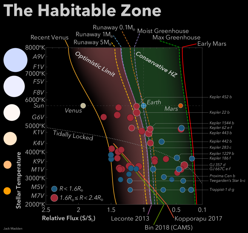
Our search for life beyond the Solar System is focused on the habitable zone. This zone is the area around a star in which a terrestrial planet could sustain liquid water on its surface. The boundaries of the habitable zone have gone through many recalculations since the 1960s (Kasting et al., 1993; Kopparapu et al., 2013; Leconte et al., 2013a ; Ramirez and Kaltenegger, 2017; Bin et al., 2018; Kopparapu et al., 2017; Gomez-Leal et al., 2019), but roughly speaking at relative fluxes between Earth and Mars we have a good understanding of how a planet here could maintain its surface water. Venus shows evidence for past liquid water so at fluxes between Venus and Earth there is the possibility of liquid surface water but it may not be part of a stable climate (Ingersoll, 1969; Kasting et al., 1984). As shown in Figure 1.1, the habitable zone is significantly modulated by star type. The hotter the star the bluer the light hitting the planet. Bluer light has more of its energy in the visible portion of the spectrum and little in infrared allowing planets to receive more total flux from blue stars but remain the same temperature. Redder, cooler stars are the opposite. Red stars emit most of their energy in the infrared so less total flux is needed to achieve a warm surface temperature.
The light from the host star of a planet also drives the photochemistry in the atmosphere. The amount and wavelengths of ultraviolet (UV) hitting an atmosphere control the production and destruction of molecules in an atmosphere. This process controls the composition and structure of an atmosphere and greatly affects what we can see when observing an atmosphere from a telescope Rugheimer et al., 2015a .
If the conditions are just right, we may be able to see signs of life through the observation of biosignatures. This was curiously tested by Sagan et al., (1993) in which a strong case was built for the remote detection of life on Earth using a range of measurements. The biosignatures I’ll mainly be talking about in this thesis are the spectroscopic measurements of molecules in an atmosphere or on the surface that when seen together provide evidence for a biologic origin. We focus on searching for spectroscopic biosignatures because of the limitations of our current and near-future telescopes only being able to measure the bulk compositions of the atmospheres and surfaces of distant planets.
Commonly mentioned biosignatures include the disequilibrium chemistry of oxidizing and reducing gases in an atmosphere suggesting a constant biotic source of one or more of the gases. Oxygen (O2), when present with methane (CH4) will eventually break down into carbon dioxide (CO2) and water (H2O). Methane can occur in significant quantities abiotically but for oxygen, large quantities can be produced quickly through mainly biologic sources. Seeing oxygen and methane together tells us that there is a constant supply of each molecule into the atmosphere. Seeing enough oxygen in the presence of methane indicates a large continuous source of oxygen which suggests a biological origin (Lederberg, 1965; Lippincott et al., 1967).
A more direct biosignature would be detecting the reflected light from the surface of the planet and matching its color to known reflectance spectra of life (Hegde and Kaltenegger, 2013). The vegetation red-edge is an example of such a biosignature (O’Malley-James and Kaltenegger, 2018b ). Many photosynthesizing organisms absorb visible light but reflect infrared light. The spectral boundary of this transition is often very distinct and is a strong indicator of life.
3 The Color of Habitability
The dark blue of an ocean, the verdant green of a forest, the faint reds in oxygen, and the heat-absorbing properties of carbon dioxide and methane. Life as we know it comes with a variety of unique colors and effects on light that, when seen in combination, provide strong evidence for biological activity. However, the challenge of making these spectroscopic observations is immense. With a vast quantity of exoplanets to choose from and more being discovered daily, the focus is now on preparing observational tools and models with the express purpose of finding life (Council, 2010).
Like any scientific endeavor, there is a theoretical approach and experimental approach that work in tandem to advance our understanding. The experimental approach to finding life involves building larger telescopes with more sensitive instruments and attempting observations of biosignatures. The theoretical approach includes building an understanding of the types of observations to make, potential biosignatures, and which places we should be looking. The testing of this theoretical work is done through forward and inverse modeling. Inverse modeling takes observations and attempts to reconstruct the source using a library of references and our understanding of climate. We have an accurate enough idea of what different molecules look like to see an atmosphere with a complex soup of elements floating around and understand its composition through inverse modeling. Inverse modeling requires observations to be made in the first place, which we do not yet have for habitable zone planets. In lieu of observational data, forward modeling takes our understanding of climate and chemistry to create novel simulations of planets allowing us to imagine which types of environments could exist.
4 Forward modeling
Forward modeling gives us insight into the types of planets that could exist within our understanding of physics. Through the process of exploring large parameter spaces, we can discover what makes worlds suitable for life and which biosignatures are most likely to be present. When it comes to modeling entire planets there are a lot of parameters available to us. Models tend to make deliberate assumptions to assure simulations run quickly while remaining accurate. The goal is to simulate climate, not weather, as many small scale atmospheric features can be ignored leaving general processes that keep an atmosphere stable.
One major simplification that can be taken advantage of is reducing the dimensionality of the model. Instead of modeling the entire atmosphere of a planet only a single vertical dimension of the atmosphere is simulated. For these 1D models, the parameters and calculations are constructed to provide an approximate look at the atmosphere as if the planet was modeled in 3D then averaged. Reducing the simulation to one dimension dramatically increases the speed of the model, but sacrifices a detailed understanding of the planet and limits where the model can be applied. One-dimensional models are best used to explore massive parameter spaces for trends in climate because of their ability to quickly model the average climate of a planet using a wide range of free parameters. While each individual simulation may not be applicable to a specific situation, the result of hundreds of models with slightly altered parameters reveals the strength and direction of an effect on climate.
In the search for habitable planets, the parameters we are interested in exploring are centered around maintaining temperatures and pressures suitable for liquid surface water. This may include altering planet-star distance, surface pressure, greenhouse gas abundance, surface albedo, or star type, among many others (Kozakis et al., 2018; Kozakis and Kaltenegger, 2019; O’Malley-James and Kaltenegger, 2018b ; Rugheimer et al., 2015b ). By exploring how these parameters affect the climate of a planet in the habitable zone of its host star, we can determine where best to look for habitable planets, what their atmospheres will look like, and which exoplanets we have found may be the best targets for intensive study. Once we have atmospheric data from a planet, we can also use our models to learn more about a planet’s climate than can be directly observed.
The primary code used in this thesis for atmosphere modeling is based on updated versions of a 1D climate (Kasting and Ackerman, 1986; Pavlov et al., 2000; Haqq-Misra et al., 2008), and a 1D photochemistry model (Pavlov and Kasting, 2002; Segura et al., 2005, 2007). This code has a long history of being used for exoplanet modeling and adaptations have been used in the most cited constructions of the habitable zone (Kasting et al., 1993; Kopparapu et al., 2013).
5 Thesis work summary
Beginning with Madden and Kaltenegger, (2018) in chapter 2 this thesis will start by looking at how we have been able to use the bodies in our Solar System as a reference guide for exploring exoplanets. In chapter 3, Madden and Kaltenegger, 2020b will show how surface albedo influences the climate of potentially habitable planets. We will take a break from exoplanet science with Madden et al., (2020) in chapter 4 by examining how virtual reality can be used in physics and astronomy education before getting back to Madden and Kaltenegger, 2020a in chapter 5 to look at the reflection and emission spectra of exoplanets with different surfaces.
5.1 The (exo)Solar System
The Solar System contains a wide variety of bodies from dusty red Mars and icy white moons to orange gas giants and a very special green planet with a blue sky. We have a much more complete understanding of the bodies in our Solar System compared to any exoplanet. By treating the spectra and albedos of objects in our Solar System as exoplanets we can create a reference guide for comparing new observations of exoplanets to bodies we know well.
In Madden and Kaltenegger, (2018), we used past observations to calculate the geometric albedos and spectra for 19 different Solar System bodies as if they orbited F, G, K, and M-stars. This allowed us to create a large database of absolute spectra for use as references in the planning and follow-up observations of large ground-based and space-based telescopes. We also examined the photometric colors of each object as we changed its host star. As a result, we determined the optimal filters in the visible and near-IR to use in order to distinguish the bodies by surface type (rocky, icy, or gaseous) depending on the host star type.
We gathered data from many sources (Lundock et al., 2009; Spencer, 1987; Filacchione et al., 2012; Fanale et al., 1974; Mallama, 2017; McCord and Westphal, 1971; Lorenzi et al., 2016; Protopapa et al., 2008; Meadows, 2006; Pollack et al., 1978) in the range from 0.45-2.5 microns for our calculations. Much of the data was relatively calibrated and required additional work to calculate the absolute values for the spectra and geometric albedos. During this process, we noted several studies that contained data that were not reduced properly or contained observation contamination previously unnoticed. After calculating a reliable set of spectra, geometric albedos, and colors for all 19 objects in our study we could then simulate their observations as exoplanets around star types other than our Sun.
Along with producing a catalog of simulated observations of the Solar System we found interesting results by looking at the data holistically. We noted that the color combination of J-K and R-J was the optimal combination in this wavelength range using standard colors to distinguish the surface types between rocky, icy, and gaseous (see also Krissansen-Totton et al., 2016; Cahoy et al., 2010; Lundock et al., 2009; Traub, 2003). This was also true independent of star type and resolution. We also observed that the CO2 atmosphere of Venus positioned it within the icy looking objects using this color combination, and positioned the Earth within the rocky objects despite the majority of its surface being covered with water.
A catalog of these spectra and albedos allows for observation planning and comparative planetology between exoplanets and objects in our Solar System (Krissansen-Totton et al., 2016; Traub, 2003). Simulated observations can be made with this data for different telescopes to gather statistics for planning and retrieval. Once observations of exoplanets are made, this catalog can be used in comparison to determine its closest analog in our Solar System. We have also shown that a simple determination of surface type can be achieved using broad filters and low resolution, opening up the possibility of smaller telescopes being able to contribute to the classification of exoplanets.
5.2 Climate and Photochemistry Modeling
After looking at examples in our Solar System, the next step in understanding terrestrial exoplanets is to model their potential climates. A 1D code has the benefit of rapid processing over 3D models, meaning a large parameter space can be explored to first order. Since the true climates of exoplanets remain unknown, the first-order exploration with 1D models is a process that will provide breadth without detailing our results beyond detection capabilities.
The 1D model we have been using and updating is a coupled climate and photochemistry model. This allows for the simulation of atmospheres around stars unlike our Sun where the UV environment is significantly different. The code iterates between balancing the pressure, temperature, and distribution of molecules with the photochemistry induced by an input stellar spectrum.
We have made substantial updates to this code’s usability and physics. It is now possible to parallelize the code across all available CPUs and automate the input file generation allowing for rapid development and deployment of parameter searches. The data handling of the code has also been streamlined to convert the data for input into a code used for observational analysis. In addition to improvements that reduce project run-time, new physics has been added to the model. With the added functionality to treat the surface as a wavelength-dependent albedo instead of a constant value, we have opened a new parameter space and begun exploring it.
Several new stellar spectra have also been added. Stellar activity and UV can have a large impact on a planet’s atmosphere even when the flux differences seem small (Rugheimer et al., 2015b ). More accurate models of the stars used in the code provide needed confidence for analyzing the output of photochemically altered species. This issue is particularly in need of attention for M-stars and well-studied systems such as Proxima Centauri and Trappist-1 due to the relatively high levels of activity of cooler stars.
5.3 Surfaces of Habitable Exoplanets
With an updated 1D code, there have been several avenues opened to understand habitability in more detail. In Madden and Kaltenegger, 2020b we take advantage of these updates by looking at the effect of surface color on habitability across star type.
Surface reflection plays a critical role in a planet’s climate due to the varying reflection of incoming starlight on the surface depending on the surface composition. 1D models commonly used to simulate terrestrial exoplanet atmospheres, such as ExoPrime and ATMOS (Segura et al., 2010, 2005, 2003; Arney et al., 2016; Rugheimer and Kaltenegger, 2018; Rugheimer et al., 2013), use a single, wavelength-independent albedo value for the planet, which has been calibrated to reproduce present-day Earth conditions for present-day Sun-like irradiance.
Even though this average value for Earth’s albedo is well calibrated to reproduce a similar climate to the wavelength-dependent albedo for present-day Earth orbiting the Sun, the particular average value will vary strongly if the incident stellar SED changes from a Sun-analog to a cool M-star or hotter F-star. For example, the cooling ice-albedo feedback is smaller for M-stars than for G-stars because ice reflects strongest in the visible shortwave region, whereas cool M-stars emit most of their energy in the red part of the spectrum (Shields et al., 2013). The climate conditions driving the snowball-deglaciation loop in models show a dependence on the stellar type, which has an impact on long-term sustained surface habitability (Shields et al., 2014). This match or mismatch of the surface albedo to the SED of a star can lead to a strong difference in heating or cooling of the planet.
No study has explored the feedback of a range of different surfaces on the climate, photochemistry, surface habitability, and the resulting spectra of terrestrial planets in the HZ orbiting a wide range of stellar host stars. The modeled climate of a planet with a flat surface albedo only responds to differences in the total incident flux received, whereas a planet with a non-flat surface albedo responds to the wavelength dependence of that flux. Thus a wavelength-dependent surface albedo is critical to assess the differing efficiencies of incoming stellar SED to heat or cool the planet. Depending on the surface, the effectiveness changes, and can not be captured with one single value for the albedo at all wavelengths for stars with different SEDs.
5.4 Eyes on atmosphere
A major component of forward modeling is linking the simulations to real observations. After parameters are decided and a planet is constructed within the model we can take the output and calculate what the planet’s spectra would look like from Earth. By taking advantage of the speed 1D models offer we can calculate spectra for hundreds of planets to build a database of references for use in other aspects of exoplanet science (Lin and Kaltenegger, 2020; Kaltenegger et al., 2020; Kozakis et al., 2020). Simulated spectra can be used in planning and optimizing observations, training atmospheric retrieval algorithms, and provides a field guide for comparison to real observations.
In Madden and Kaltenegger, 2020a , we follow from the previous modeling work for different surfaces (Madden and Kaltenegger, 2020b ) and use a radiative transfer code to generate reflectance and emission spectra for each case. This allowed us to cross-compare the spectra to show which cases show the most distinctive features and provide the best opportunity to observe biosignatures. The database of spectra we have created is made from planet models with 30 different surfaces around 12 types of host stars. Our high resolution is applicable to the observations that will be made in the near future by ground-based telescopes like the Giant Magellan Telescope (GMT), Thirty Meter Telescope (TMT), and Extremely Large Telescope (ELT), and concept telescopes like HabEx, LUVOIR, and Origins (Arney et al., 2018; Snellen et al., 2017, 2015; Rodler and López-Morales, 2014; Brogi et al., 2014; Fischer et al., 2016; Lopez-Morales et al., 2019).
As we make our first attempts at finding evidence for life in the atmospheres of potentially habitable planets we must have strong theoretical backing to support the data. Building an understanding of our Solar System, exploring the effects of surface albedo, and calculating new spectra for future reference contribute to the search for life by building up a stronger theoretical framework around the observations we plan to make.
5.5 Physics Education Research
Along with exoplanet science, this thesis contains research on education in astronomy using virtual reality. Generally regarded as the oldest natural science, astronomy education has come a long way. Recently, virtual reality (VR) has entered the scene as a potential way to immerse students in a learning experience like never before. Before schools and universities make a large investment in VR technology research needs to be done to determine the circumstances in which VR is beneficial, to what degree it is beneficial and simply if it is beneficial at all for students.
VR allows users to enter a simulated environment where perspectives, physics, time, and space can be altered to a point only limited by the imagination of the creators. This sandbox allows for educators to build an interactive classroom capable of showing concepts and phenomena in ways never before accessible in a traditional classroom. Just like how desktop computers have been able to show students simulations and play with physics in a virtual program, VR is equally capable of this with the additional feature of 3D immersion in the program. But does that make for a better learning experience?
To test this, we built an immersive 3D environment to recreate the classic Moon phase demonstration involving a ball and a light source to simulate the Moon phases. The environment was build by our team using the Unity game engine for the Oculus Rift. A detailed Earth-Moon-Sun system was created with accurate orbits, inclination, surface textures, and background stars. The simulation allowed users to alter time by dragging the Moon through its phases from three different vantage points in the system.
After months of program development, we recruited participants to take a test on their Moon phase knowledge before experiencing our VR simulation and afterward to compare with results to students who experienced the traditional analog demonstration. This work provides one of the most comprehensive looks into VR as a teaching tool in physics and provides detailed guidelines for conducting future research in this field and recommendations for using VR in the classroom.
![[Uncaptioned image]](/html/2010.05046/assets/art/MFA_d10.jpg)
Chapter 2 A Catalog of Spectra, Albedos, and Colors of Solar System Bodies for Exoplanet Comparison
This thesis chapter originally appeared in the literature as
J. Madden and L. Kaltenegger, Astrobiology, Volume 18, Issue 12, pp.1559-1573 (2018)
Abstract
We present a catalog of spectra and geometric albedos, representative of the different types of Solar System bodies, from 0.45 to 2.5 microns. We analyzed published calibrated, un-calibrated spectra, and albedos for Solar System objects and derived a set of reference spectra and reference albedo for 19 objects that are representative of the diversity of bodies in our Solar System. We also identified previously published data that appears contaminated. Our catalog provides a baseline for comparison of exoplanet observations to 19 bodies in our own Solar System, which can assist in the prioritization of exoplanets for time intensive follow-up with next generation Extremely Large Telescopes (ELTs) and space based direct observation missions. Using high and low-resolution spectra of these Solar System objects, we also derive colors for these bodies and explore how a color-color diagram could be used to initially distinguish between rocky, icy, and gaseous exoplanets. We explore how the colors of Solar System analog bodies would change when orbiting different host stars. This catalog of Solar System reference spectra and albedos is available for download through the Carl Sagan Institute.
1 Introduction
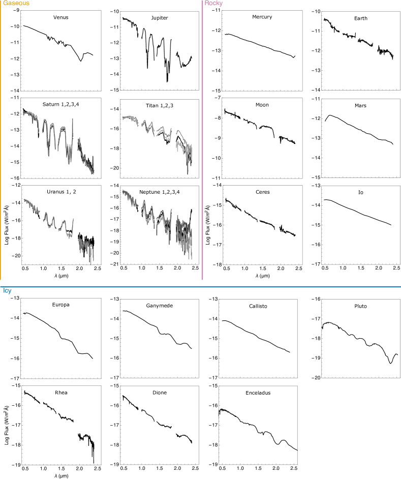
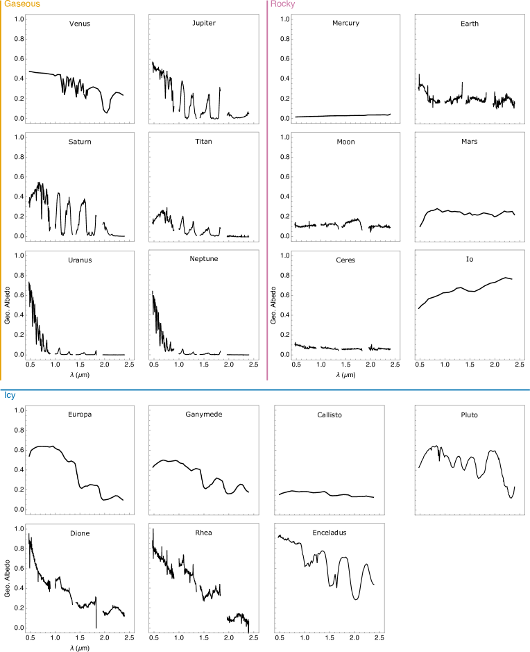
The first spectra of extrasolar planets have already been observed for gaseous bodies (e.g. Dyudina et al., 2016; Kreidberg et al., 2014; Mesa et al., 2016; Sing et al., 2016; Snellen et al., 2010). To aid in comparative planetology exoplanet observations will require an accurate set of disk-integrated reference spectra, and albedos of Solar System objects. To establish this catalog for the solar system we use disk-integrated spectra from several sources. We use un-calibrated and calibrated spectra as well as albedos when available from the literature to compile our reference catalog. About half of the spectra and albedos we derive in this paper are based on un-calibrated observations obtained from the Tohoku-Hiroshima-Nagoya Planetary Spectral Library (THN-PSL)(Lundock et al., 2009), which provides a large coherent dataset of un-calibrated data taken with the same telescope. Our analysis shows contamination of part of that dataset, as discussed in section 2.1 and 2.2, therefore we only include a subset of their data in our catalog (see discussion 4.3). This paper provides the first catalog of calibrated spectra (Fig. 2.1) and geometric albedos (Fig. 2.2) of 19 bodies in our Solar System, representative of a wide range of object types: all 8 planets, 9 moons (representing, icy, rocky, and gaseous moons), and 2 dwarf planets (Ceres in the Asteroid belt and Pluto in the Kuiper belt). This catalog is available through the Carl Sagan Institute111www.carlsaganinstitute.org/data/ to enable comparative planetology beyond our Solar System. Several teams have shown that photometric colors of planetary bodies can be used to initially distinguish between icy, rocky, and gaseous surface types Krissansen-Totton et al., (2016); Cahoy et al., (2010); Lundock et al., (2009); Traub, (2003) and that models of habitable worlds lie in a certain color space (Krissansen-Totton et al., 2016; Hegde and Kaltenegger, 2013; Traub, 2003). We expand these earlier analyses from a smaller sample of Solar System objects to 19 Solar System bodies in our catalog, which represent the diversity of bodies in our Solar System. In addition, we explore the influences of spectral resolution on characterization of planets in a color-color diagram by creating low resolution versions of our data. Using the derived albedos, we also explore how colors of analog planets would change if they were orbiting other host stars. Section 2 of this paper describes our methods to identify contamination in the THN-PSL data, derive calibrated spectra, albedos, and colors from the un-calibrated THN-PSL data and how we model the colors of the objects around the Sun and other host stars. Section 3 presents our results, Section 4 discusses our catalog, and Section 5 summarizes our findings.
2 Method
We first discuss our analysis of the THN-PSL data and how we identified contaminated data in detail, then discuss how we derived spectra and albedo from the uncontaminated data. Finally we discuss spectra and albedo from other data sources for our catalog.
2.1 Calibrating the Spectra of Solar System Bodies from the THN-PSL
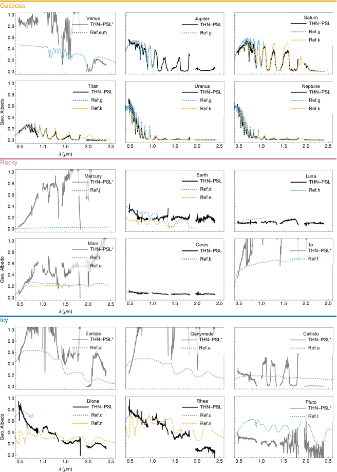
The THN-PSL is a collection of observations of 38 spectra for 18 Solar System objects observed over the course of several months in 2008. The spectra of one of the objects, Callisto, was contaminated and could not be re-observed, while the spectrum for Pluto in the database is a composite spectrum of both Pluto and Charon. We analyzed the data for the 16 remaining Solar System objects for additional contamination and found 6 apparently contaminated objects among them, leaving 10 objects in the database that do not appear contaminated. Their albedos are similar to published values in the literature for the wavelength range such data is available for. We show the derived albedos for both contaminated and uncontaminated data from the database in Fig. 2.3, compared to available values from the literature for these bodies.
The THN-PSL data were taken in 2008 using the TRISPEC instrument while on the Kanata Telescope at the Higashi-Hiroshima observatory. TRISPEC (Watanabe et al., 2005) splits light into one visible channel and two near-infrared channels giving a wavelength range of 0.45-2.5 . The optical band covered 0.45-0.9 and had a resolution of . The first IR channel has a coverage from 0.9-1.85 and had a resolution of . The second IR channel has a coverage from 1.85-2.5 and had a resolution of . Note that the slit subtends 4.5 arcseconds by 7 arcmin meaning that spectra for larger bodies such as Saturn and Jupiter were not disk integrated (see discussion). As discussed in the original paper, all spectra are unreliable below 0.47 and between 0.9-1.0 from a dichroic coating problem with the beam splitters. Near 1.4 and 1.8 the Earth’s water absorption degrades the quality and beyond 2.4 thermal contamination is an issue. These wavelength regions are grayed out in all relevant figures in our paper but do not influence our color analysis, due to the choice of filters. The raw data available for download includes all data points. The THN-PSL paper discusses several initial observations of moons that were contaminated with light from their host planet rendering their spectra inaccurate (080505 Callisto, 081125 Dione, 080506 Io, and 080506 Rhea). These objects (with the exception of Callisto) were observed again and the extra light was removed in a different fashion to more accurately correct the spectra (Lundock et al., 2009). Callisto was not re-observed and therefore the THN-PSL Calisto data remained contaminated (Fig. 2.3). The fluxes of the published THN-PSL observations were not calibrated but arbitrary normalized to the value of 1 at 0.7. This makes the dataset generally useful to compare the colors of the uncontaminated objects, as shown in the original paper, but limits the data’s usefulness as reference for extrasolar planet observations because geometric albedos can only be derived from calibrated spectra. The conversion factors used in the original publication were not available (Ramsey Lundock, private communication). However, in addition to the V magnitude, the THN-PSL gives the color differences: V-R, R-I, R-J, J-K, and H-Ks for each observation, providing the R, I, and J magnitudes. Therefore, we used the published V, R, I, and J magnitudes to derive the conversion factor for each spectrum to match the published color magnitudes and to calibrate the THN-PSL observations.
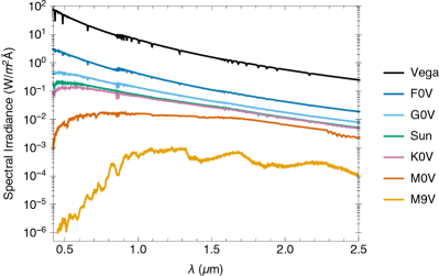
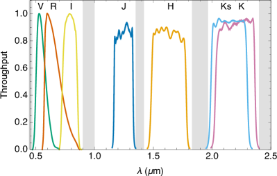
We define the conversion factor such that where and are the normalized and absolute spectra respectively. Adapting the method outlined in Fukugita et al., (1995) the magnitude in a single band using the filter response, V, and the spectrum of Vega, , is given by equation (1). The spectrum of Vega, (Bohlin, 2014)222www.stsci.edu/hst/observatory/crds/calspec.html (alpha_lyr_stis_008.fits) as well as the filter responses, are the same as in the THN-PSL publication and shown in Fig. 2.5 and Fig. 2.5 respectively. The filters we used are V (Johnson and Morgan, 1953); R and I (Bessell, 1979; Cousins, 1976); J, H, K, and Ks (Tokunaga et al., 2002). Since the THN-PSL paper recorded the V, R, I, and J color magnitudes for each object we derive the conversion factor to obtain each magnitude and average them to obtain k. For example, we substitute in equation (2) and isolate as shown in equation (3) to calculate the conversion factors for the V band. The conversion factors for each band for a single object were averaged and used to calibrate the normalized spectra.
| (2.1) | ||||
| (2.2) | ||||
| (2.3) | ||||
| (2.4) |
We used this method to calibrate the THN-PSL data for each object. When comparing the coefficient of variation () of the conversion factors for each body we found that the data showed two distinct groups, one with a greater than 14% and another with a smaller than 6%. We use that distinction to set the level of the conversion factor for uncontaminated spectra to over the different filter bins. If the value was in the second group , the data is flagged as contaminated and not used in our catalog. The nature of this contamination is unclear, it could be photometric error during the observation, excess light from the host planet or other effects that influenced the observations. The values calculated for the , , , , , and the for each observation is given in Table 2.1.
| Name | Obs. Date | |||||||
| Uncontaminated ( <6% and albedo <1) | ||||||||
| Ceres | 11/25/08 | 8.27E-16 | 8.27E-16 | 8.45E-16 | 8.36E-16 | 8.34E-16 | 8.44E-18 | 1.01% |
| Dione | 5/5/08 | 1.34E-16 | 1.34E-16 | 1.35E-16 | 1.34E-16 | 1.34E-16 | 6.75E-19 | 0.50% |
| Earth | 11/21/08 | 1.48E-11 | 1.48E-11 | 1.50E-11 | 1.50E-11 | 1.49E-11 | 1.14E-13 | 0.77% |
| Jupiter | 5/7/08 | 2.17E-11 | 2.16E-11 | 2.08E-11 | 2.19E-11 | 2.15E-11 | 5.03E-13 | 2.34% |
| Moon | 11/21/08 | 1.49E-08 | 1.49E-08 | 1.54E-08 | 1.51E-08 | 1.51E-08 | 2.27E-10 | 1.50% |
| Neptune 1 | 5/7/08 | 5.28E-16 | 5.38E-16 | 4.89E-16 | 5.25E-16 | 5.20E-16 | 2.14E-17 | 4.11% |
| Neptune 2 | 11/20/08 | 4.44E-16 | 4.53E-16 | 4.33E-16 | 4.42E-16 | 4.43E-16 | 8.44E-18 | 1.90% |
| Neptune 3 | 11/25/08 | 2.96E-16 | 3.02E-16 | 2.86E-16 | 2.97E-16 | 2.95E-16 | 6.51E-18 | 2.20% |
| Neptune 4 | 11/26/08 | 7.80E-16 | 7.94E-16 | 7.46E-16 | 7.76E-16 | 7.74E-16 | 2.00E-17 | 2.59% |
| Pluto | 5/11/08 | 2.67E-18 | 2.67E-18 | 2.70E-18 | 2.71E-18 | 2.69E-18 | 2.10E-20 | 0.78% |
| Rhea | 11/25/08 | 2.72E-16 | 2.71E-16 | 2.73E-16 | 2.73E-16 | 2.72E-16 | 1.14E-18 | 0.42% |
| Saturn 1 | 5/5/08 | 8.29E-13 | 8.31E-13 | 7.86E-13 | 8.49E-13 | 8.24E-13 | 2.70E-14 | 3.28% |
| Saturn 2 | 11/19/08 | 1.11E-12 | 1.10E-12 | 1.05E-12 | 1.13E-12 | 1.10E-12 | 3.44E-14 | 3.14% |
| Saturn 3 | 11/19/08 | 1.00E-12 | 9.97E-13 | 9.57E-13 | 1.02E-12 | 9.94E-13 | 2.68E-14 | 2.70% |
| Saturn 4 | 11/22/08 | 7.57E-13 | 7.52E-13 | 7.21E-13 | 7.62E-13 | 7.48E-13 | 1.81E-14 | 2.42% |
| Titan 1 | 5/5/08 | 1.12E-15 | 1.13E-15 | 1.09E-15 | 1.13E-15 | 1.12E-15 | 1.79E-17 | 1.60% |
| Titan 2 | 5/6/08 | 1.74E-15 | 1.72E-15 | 1.70E-15 | 1.76E-15 | 1.73E-15 | 2.47E-17 | 1.43% |
| Titan 3 | 11/24/08 | 1.17E-15 | 1.16E-15 | 1.12E-15 | 1.18E-15 | 1.16E-15 | 2.45E-17 | 2.11% |
| Uranus 1 | 5/11/08 | 3.04E-15 | 3.12E-15 | 2.76E-15 | 3.00E-15 | 2.98E-15 | 1.53E-16 | 5.12% |
| Uranus 2 | 11/20/08 | 3.30E-15 | 3.37E-15 | 3.19E-15 | 3.26E-15 | 3.28E-15 | 7.48E-17 | 2.28% |
| Contaminated (albedo >1) | ||||||||
| Callisto | 5/5/08 | 7.38E-15 | 7.36E-15 | 6.90E-15 | 7.55E-15 | 7.30E-15 | 2.78E-16 | 3.81% |
| Europa | 5/7/08 | 2.47E-14 | 2.46E-14 | 2.58E-14 | 2.48E-14 | 2.49E-14 | 5.57E-16 | 2.24% |
| Ganymede | 11/26/08 | 4.20E-14 | 4.17E-14 | 4.52E-14 | 4.26E-14 | 4.29E-14 | 1.62E-15 | 3.79% |
| Io | 11/26/08 | 1.26E-14 | 1.25E-14 | 1.41E-14 | 1.29E-14 | 1.31E-14 | 7.45E-16 | 5.70% |
| Mars | 5/12/08 | 1.59E-12 | 1.57E-12 | 1.73E-12 | 1.60E-12 | 1.62E-12 | 7.56E-14 | 4.67% |
| Mercury | 5/11/08 | 7.18E-12 | 7.12E-12 | 8.02E-12 | 7.31E-12 | 7.41E-12 | 4.16E-13 | 5.61% |
| Venus | 11/20/08 | 1.40E-10 | 1.39E-10 | 1.43E-10 | 1.39E-10 | 1.40E-10 | 2.08E-12 | 1.49% |
| Contaminated (CV >14%) | ||||||||
| Earth | 5/11/08 | 1.84E-11 | 1.79E-11 | 1.62E-11 | 2.26E-11 | 1.88E-11 | 2.71E-12 | 14.43% |
| Moon | 11/21/08 | 2.08E-08 | 1.84E-08 | 2.10E-08 | 3.04E-08 | 2.26E-08 | 5.33E-09 | 23.55% |
| Uranus | 5/7/08 | 3.28E-15 | 3.22E-15 | 2.60E-15 | 7.30E-16 | 2.46E-15 | 1.19E-15 | 48.52% |
2.2 Albedos of Solar System Bodies
We then derive the geometric albedo from the calibrated spectra as a second part of our analysis (see Table 2.2 and Table 2.3 for references) by dividing the observed flux of the Solar System bodies by the solar flux and accounting for the observation geometry as given in equation (5) (de Vaucouleurs, 1964).
| (2.5) |
Where d is the separation between Earth and the body, ab the distance between the Sun and the body at the time of observation, and the semi major axis of Earth. and are the fluxes from the Sun seen from Earth and the body seen from Earth respectively, is the radius of the body being observed, and is the value of the phase function at the point in time the observation was taken. For , we used the standard STIS Sun spectrum (Bohlin et al., 2001)333www.stsci.edu/hst/observatory/crds/calspec.html (sun_reference_stis_002.fits) shown in Fig. 2.5. If the geometric albedo exceeds 1, the data is flagged as contaminated and not used in our catalog. Note that we also compared the spectra that were flagged as contaminated in this 2-step analysis with the available data and models from other groups (Fig. 2.3). All flagged spectra show a strong difference in albedo for these bodies observed by other teams, supporting our analysis method (see Fig. 2.3).
| Name | Obs. Date | V Mag. | Phase | Albedo | |||||
|---|---|---|---|---|---|---|---|---|---|
| (AU) | (AU) | (km) | (deg.) | Ref. | Ref. | ||||
| Ceres | 11/25/08 | 8.40 | 2.405 | 2.558 | 470 | 23 | 0.34(5) | a | a |
| Dione | 5/5/08 | 10.40 | 8.97 | 9.298 | 560 | 6 | 0.88(3) | b | l,v |
| Earth | 11/21/08 | -2.50 | 0.0026† | 0.988† | 6378 | 70 | 0.5 | c | m,n |
| Jupiter | 5/7/08 | -2.40 | 4.68 | 5.199 | 71492 | 10 | 0.91(8) | d | o |
| Moon | 11/21/08 | -9.30 | 0.0026 | 0.988 | 1738 | 108 | 0.05(1) | e | e |
| Neptune 1 | 5/7/08 | 7.90 | 30.14 | 30.04 | 24766 | 2 | 1 | f | o,p |
| Neptune 2 | 11/20/08 | 7.90 | 30.145 | 30.03 | 24766 | 2 | 1 | f | o,p |
| Neptune 3 | 11/25/08 | 7.90 | 30.23 | 30.03 | 24766 | 2 | 1 | f | o,p |
| Neptune 4 | 11/26/08 | 7.90 | 30.247 | 30.03 | 24766 | 2 | 1 | f | o,p |
| Pluto* | 5/11/08 | 15.00 | 30.72 | 31.455 | 1150 | 1 | 1 | q | |
| Rhea | 11/25/08 | 9.90 | 9.591 | 9.36 | 764 | 6 | 0.87(2) | b | l,v |
| Saturn 1 | 5/5/08 | 1.00 | 8.97 | 9.296 | 60268 | 6 | 0.76(3) | d | o,p |
| Saturn 2 | 11/19/08 | 1.20 | 9.685 | 9.356 | 60268 | 6 | 1 | d | o,p |
| Saturn 3 | 11/19/08 | 1.20 | 9.685 | 9.356 | 60268 | 6 | 0.76(3) | d | o,p |
| Saturn 4 | 11/22/08 | 1.20 | 9.6385 | 9.359 | 60268 | 6 | 0.76(3) | d | o,p |
| Titan 1 | 5/5/08 | 8.40 | 8.97 | 9.3 | 2575 | 6 | 0.98(3) | g | o,p |
| Titan 2 | 5/6/08 | 8.40 | 8.97 | 9.3 | 2575 | 6 | 0.98(3) | g | o,p |
| Titan 3 | 11/24/08 | 8.60 | 9.5947 | 9.364 | 2575 | 6 | 0.98(3) | g | o,p |
| Uranus 1 | 5/11/08 | 5.90 | 20.66 | 20.097 | 25559 | 2 | 1 | f | o,p |
| Uranus 2 | 11/20/08 | 5.80 | 19.742 | 20.097 | 25559 | 3 | 1 | f | o,p |
| Name | Obs. Date | V Mag. | Phase | Albedo | |||||
|---|---|---|---|---|---|---|---|---|---|
| (AU) | (AU) | (km) | (deg.) | Ref. | Ref. | ||||
| Callisto* | 5/5/08 | 6.30 | 4.73 | 5.214 | 2410 | 10 | 0.60(2) | h | r,s |
| Europa | 5/7/08 | 5.60 | 4.69 | 5.195 | 1565 | 10 | 0.88(5) | i,b | i,r,s |
| Ganymede | 11/26/08 | 5.40 | 5.7518 | 5.12066 | 2634 | 8 | 0.80(5) | h | r,s |
| Io | 11/26/08 | 5.80 | 5.7556 | 5.12348 | 1821 | 8 | 0.87(5) | j | s,t |
| Mars | 5/12/08 | 1.30 | 1.68 | 1.6676 | 3397 | 35 | 0.58(5) | d | u,n |
| Mercury | 5/11/08 | 0.00 | 0.99 | 0.37547 | 2440 | 96 | 0.11(5) | d,k | k,x |
| Venus | 11/20/08 | -4.20 | 1.077 | 0.72556 | 6052 | 63 | 0.4(1) | d | n,m |
References for Table 2.2 and 2.3: a(Reddy et al., 2015), b(Buratti and Veverka, 1983), c(Goode et al., 2001), d(Irvine et al., 1968), e(Lane and Irvine, 1973), f(Pollack et al., 1986), g(Tomasko and Smith, 1982), h(Squyres and Veverka, 1981), i(Buratti and Veverka, 1983), j(Simonelli and Veverka, 1984), k(Mallama et al., 2002), l(Noll et al., 1997), m(Kaltenegger et al., 2010), n(Meadows, 2006), o(Karkoschka, 1998), p(Fink and Larson, 1979), q(Lorenzi et al., 2016; Protopapa et al., 2008) r(Spencer, 1987), s(Spencer et al., 1995) t(Fanale et al., 1974) u(McCord and Westphal, 1971), v(Cassini VIMS - NASA PDS), w(Pollack et al., 1978), x(Mallama, 2017)
2.3 Using colors to characterize planets
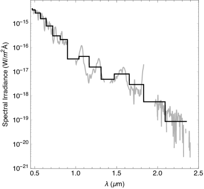
We use a standard astronomy tool, a color-color diagram, to analyze if we can distinguish Solar System bodies based on their colors and what effect resolution and filter choice has on this analysis. Several teams have shown that photometric colors of planetary bodies can be used to initially distinguish between icy, rocky, and gaseous surface types (Krissansen-Totton et al., 2016; Cahoy et al., 2010; Lundock et al., 2009; Traub, 2003). We calculated the colors from high and low-resolution spectra to mimicearly results from exoplanet observations as well as explored the effect of spectral resolution on the colors and their interpretation.The error for colors derived from the THN-PSL data was calculated by adding the errors used by Lundock et al., (2009) and the error accumulated through the conversion process of 6% in the value. This gives and for the error values. We reduce the high-resolution data of to in order to mimic colors that are generated from low-resolution spectra as shown in Fig. 2.6. The colors at high resolutions were used to determine the best color-color combination for surface and atmospheric characterization, a process that was repeated for colors derived from low resolution spectra.
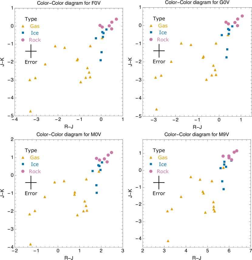
We also explored how to characterize Solar System analog planets around other host stars using their colors by placing the bodies at an equivalent
orbital distance around different host stars (F0V, G0V, M0V, and M9V). We used stellar spectra for the host stars from the Castelli and Kurucz Atlas (Castelli and Kurucz, 2004)444www.stsci.edu/hst/observatory/crds/castelli kurucz atlas.html (F0V, G0V, K0V, M0V) and the PHOENIX library (Husser et al., 2013)555 http://phoenix.astro.physik.uni-goettingen.de (M9V) (Fig. 2.5). As a first order approximation, we have assumed that the albedo of the object would not change under this new incoming stellar flux (See discussion).
3 Results
3.1 A spectra and albedo catalog of a diverse set of Solar System Objects
We assembled a reference catalog of 19 bodies in our Solar System as a baseline for comparison to upcoming exoplanet observations. To provide a wide range of Solar System bodies in our catalog we compiled and analyzed data from un-calibrated and calibrated spectra of previously published disk-integrated observations. Our catalog contains spectra and geometric albedo of the 8 planets: Mercury (Mallama, 2017), Venus (Meadows, 2006; Pollack et al., 1978), Earth (Lundock et al., 2009), Mars (McCord and Westphal, 1971), Jupiter, Saturn, Uranus, and Neptune (Lundock et al., 2009). 9 moons: Io (Fanale et al., 1974), Callisto, Europa, Ganymede (Spencer, 1987), Enceladus666Data available on NASA’s Planetary Data Archive: (v1640517972_1, v1640518173_1, v1640518374_1) (Filacchione et al., 2012), Dione, Rhea, the Moon, and Titan (Lundock et al., 2009), and 2 dwarf planets: Ceres (Lundock et al., 2009) and Pluto (Lorenzi et al., 2016; Protopapa et al., 2008). For the 8 planets of the Solar System, 9 moons (Callisto, Dione, Europa, Ganymede, Io, the Moon, Rhea, Titan), and 2 dwarf planets (Ceres and Pluto) we present the absolute fluxes in Fig. 2.1 and the geometric albedos in Fig. 2.2.
3.2 Contaminated spectra in the THN-PSL dataset
When we derived the geometric albedo from the calibrated THN-PSL spectra as the second part of our analysis, we found that 6 objects (Io, Europa, Ganymede, Mercury, Mars, and Venus) display geometric albedos exceeding 1, indicating that the measurements are contaminated (see Table 2.3, Fig. 2.3). We compared the albedo of these six observations to previously published values in the literature (Mallama, 2017; Meadows, 2006; Mallama et al., 2002; Spencer et al., 1995; Spencer, 1987; Buratti and Veverka, 1983; Pollack et al., 1978; Fanale et al., 1974; McCord and Westphal, 1971) and found substantial differences over the wavelength covered by the different teams (Fig. 2.3). We list the 7 bodies with contaminated THN-PSL measurements in Table 2.3.
3.3 Spectra not flagged as contaminated in the THN-PSL dataset
Table 2.2 lists the spectra of the 10 bodies from the THN-PSL database, which were not flagged as contaminated and are part of our catalog, as well as the Pluto-Charon spectrum. It shows the properties we used to calculate their albedos, once we un-normalized the un-calibrated data as well as references to previously published albedos. Note that we did not use the THN-PSL Pluto-Charon spectrum in our analysis because it is not a Pluto spectrum. Instead we use the spectrum for Pluto published by two teams (Lorenzi et al., 2016; Protopapa et al., 2008) that cover the wavelength range requires for our analysis. We show both spectra in Fig.3 for completeness. We compared the derived albedo of the 10 bodies from the THN-PSL database, which were not flagged as contaminated, against disk-integrated spectra and albedo from observations or models in the literature for the wavelengths available. Our derived albedos are in qualitative agreement with previously published data (Fig. 2.3) for Ceres (Reddy et al., 2015); Dione and Rhea (Noll et al., 1997, Cassini VIMS,); Earth (Kaltenegger et al., 2010; Meadows, 2006); the Moon (Lane and Irvine, 1973); Jupiter, Saturn, Uranus, Neptune, and Titan (Karkoschka, 1998; Fink and Larson, 1979). We simulated their absolute fluxes with the same observation geometry as the THN-PSL spectra to be able to compare them (Fig. 2.3). Note that small changes are likely due to observation geometry as well as the changes in the atmospheres over the time between observations. Giant planets have daily variations in brightness (Belton et al., 1981). For completeness we include the THN-PSL observation of the combined spectrum of Pluto and Charon and compare it to the albedo of Pluto (Lorenzi et al., 2016; Protopapa et al., 2008). We averaged several Cassini VIMS observations together and used them as references for Rhea and Dione777Data available on NASA’s PDS: Rhea - v1498350281_1, v1579258039_1, v1579259351_1 Dione - v1549192526_1, v1549192731_1, v1549193961_1.
3.4 Using Color-color diagrams to initially characterize Solar System bodies
To qualify the Solar System objects in terms of extrasolar planet observables, we consider whether they are gaseous, icy, or rocky bodies and do not distinguish between moons and planets. Thus, Titan and Venus are both gaseous bodies in our analysis since only their atmosphere is being observed at this wavelength range. Fig. 2.7 shows the spectra as well as the colors for the three subcategories in our catalog. The top panel shows gaseous bodies: Jupiter, Saturn, Uranus, Neptune, Venus, Titan. The middle panel shows rocky bodies: Mars, Mercury, Io, Ceres, Earth, and the Moon. The bottom panel shows icy bodies: Ganymede, Dione, Rhea, Callisto, Pluto, Europa, and Enceladus. Each surface type occupies its own color space in the diagram. To explore how the resolution of the available spectra and thus the observation time available would influence this classification, we reduced the spectral resolution for all spectra to of 8.
We find that the derived colors of the Solar System bodies do not shift substantially (Fig. 2.8), showing that colors derived from high and low-resolution spectra provide similar capabilities for first order color-characterization of a Solar System object. While a slight shift occurs in the color-color diagram, the three different Solar System surface types (gaseous, rocky and icy) can still be distinguished, showing that colors from low resolution spectra can be used for first order characterization of bodies in our Solar System.
We chose a lower resolution of since the bin width near the K-band becomes larger than the K-band filter itself at lower resolutions. Bandwidth is directly proportional to the amount of light collected by a telescope and thus the time needed for observation. If low-resolution spectra could initially characterize a planet, exoplanets could be prioritized for time-intense high-resolution follow-up observations from their colors. At a lower resolution, a higher signal to noise ratio is required to achieve the same distinguishability as an observation at high resolution. The ratio of the integral uncertainties of two spectra at different resolutions, and ,
| (2.6) |
is proportional to the number of bins being integrated over, N, and the measurement uncertainty of each bin, , as shown in equation 6.
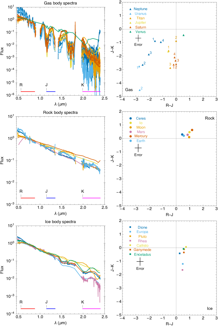
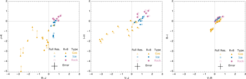
We explored different filter combinations to best distinguish between icy, gaseous and rocky bodies. We find that R-J versus J-K colors distinguish the bodies best, (see also Krissansen-Totton et al., 2016; Cahoy et al., 2010; Lundock et al., 2009; Traub, 2003). If only a smaller wavelength range is available, such as V through H or V through I, Fig. 2.8 shows which alternate filter combinations can still separate the surface types. However, Fig. 2.8 shows that a wider wavelength range improves the characterization of surfaces for Solar System objects substantially. The success of using this method to characterize the Solar System reduces with narrower wavelength coverage. Long wavelengths (J and K band) especially help distinguish different kind of Solar System bodies (Fig. 2.8). To characterize all bodies in the Solar System it is important to have wavelength coverage of the visible and near IR at a resolution that distinguishes each band.
3.5 Colors of Solar System analog bodies orbiting different host stars
To provide observers with the color-space where Solar System analog exoplanets could be found, we use the albedos shown in Fig. 2.2 to explore the colors of similar bodies orbiting different host stars. For airless bodies the albedo is a direct surface measurement, therefore that assumption should be valid for similar surface composition. For objects with substantial atmospheres that can be influenced by stellar radiation, individual models are needed to assess whether the albedo of a system’s bodies would notably change due to the different host star flux. Note that Earth’s albedo would not change significantly from F0V to M9V host stars in the wavelength range considered here (see Rugheimer et al., 2013, 2015). Fig. 2.9 shows the colors of the Solar System analog bodies orbiting other host stars. Because their albedo is assumed to be constant the shift closely mimics the shift in colors of the host star. For hotter host stars the colors shift to a bluer section of the color-color diagram (F0V). For cooler host stars the colors shift toward a redder portion of the color space (M0V, and M9V). This provides insights for observers into where the divisions in color-space of rocky, icy, and gaseous bodies lie depending on the host star’s spectral class.
4 Discussion
4.1 Change in colors of Gaseous Planets
Some gaseous bodies in the THN-PSL with multiple spectra (Uranus, Neptune, and Titan) show variations in their colors larger than the error (Fig. 2.7). Gaseous bodies are known to vary in brightness over timescales shorter than the time between these observations (Belton et al., 1981), consistent with the THN-PSL data. This indicates that any sub-divide for gaseous bodies would be challenging from their colors alone. However the K-band is also more susceptible to photometric error as discussed in the THN-PSL paper (Lundock et al., 2009), which could add to the observed differences. Multiple uncontaminated observations across the same wavelengths for rocky or icy bodies are not available in the literature, therefore we cannot assess whether a spread in colors also exists for rocky or icy bodies, independent of viewing geometry.
4.2 Non disk-integrated spectra of some objects
Due to the finite field of view of the TRISPEC instrument the observations of the Earth, Moon, Jupiter, and Saturn were not disk integrated. A disk integrated spectrum is preferred because it averages the light from the entire body instead of from a small region of its surface. The spectrograph slit was centered on the planet and aligned longitudinally for Jupiter and Saturn making the spectra as representative of the entire surface as possible. When comparing their spectra to other sources, the spectra shows a good match to disk integrated spectra (Karkoschka, 1998; Fink and Larson, 1979). This could not be done for the Moon and the Earthshine observations leading to variations in their spectra from previously published data.
4.3 Spectra derived from the THN-PSL dataset
We have used several spectra of planets and moons from the THN-PSL dataset that did not appear contaminated in our analysis. The contamination of 6 objects in the THN-PSL database raises questions about the viability of the spectra in this database in general. We compared the 10 bodies that we used in our catalog, which were not flagged as contaminated against disk-integrated spectra and albedo from observations or models in the literature. These observations or models were not available for the whole wavelength range, thus we could not compare the full wavelength range, however the range covered shows qualitative agreement with previously published data (Fig. 2.3) and thus we have included the spectra and albedos we derived from the un-calibrated THN-PSL data in our analysis. For Earth and the Moon time variability of the spectra can be explained because observations of the Earth and the Moon were not disk integrated, due to the spectrographic slit as discussed in 4.2. Note that for most solar system objects, reliable disc-averaged spectra for different times are lacking, which are observations that would be useful for future exoplanet comparisons.
4.4 Similarity of the color of water and rock
The primarily liquid water surface of the Earth is unique in the Solar System however, this is not apparent in the color-color diagrams (Fig 2.7, 2.8, and 2.9). This is because water and rock share a similar, relatively flat, albedo over the 0.5-2.5 wavelength range. This specific color-color degeneracy for rock and water can be broken if shorter wavelength observations are available (see also Krissansen-Totton et al., 2016).
4.5 Color of atmospheres appear similar to icy surfaces
Venus has the interesting position of being a rocky planet that has a gaseous appearance but lies amongst the colors of the icy bodies in the color-color diagrams. This is due to Venus having a primarily CO2 atmosphere which provides a similarly sloped albedo as ice in this wavelength range. This shows the limits of initial characterization through a color-color diagram. It will make habitability assessments from colors alone of terrestrial planets especially on the edges of their habitable zones very difficult since CO2 is likely to be present. Estimates of the effective stellar flux that reaches the planet or moon could help to disentangle the ice/CO2 degeneracy on the inner edge of the Habitable Zone. On the outer edge of the Habitable Zone both surface types should be present, CO2-rich atmospheres as well as icy bodies, therefore higher resolution spectra will be needed to break such degeneracy.
4.6 Spotting the absence of methane in a gas planet’s colors
The absence of methane in Venus’ atmosphere makes it distinguishable from the other gaseous objects in our Solar System in the color-color diagrams. More information about the atmospheric composition of exoplanets and exomoons would be needed before we can assess whether we could derive similar inferences for other planetary systems.
4.7 Colors of objects that are made of ‘dirty snow’
In the color-color diagrams, Ganymede and Callisto fall in the region between rocky and ice bodies due to their high amount of ‘dirty snow’ compared to the other bodies in the icy body category. Given the error bars in their colors, these two bodies could be placed in either the rocky or icy categories. Such rocky-icy bodies are anticipated in other planetary systems as well and should lie in the color space between the icy and rocky bodies like in our Solar System.
5 Conclusions
We present a catalog of spectra, and geometric albedos for 19 Solar System bodies, which are representative of the types of surfaces found throughout the Solar System for wavelengths from 0.45-2.5 microns. This catalog provides a baseline for comparison of exoplanet observations to the most closely studied bodies in our Solar System. The data used and created by this paper is available for download through the Carl Sagan Institute888www.carlsaganinstitute.org/data/. We show the utility of a color-color diagram to distinguish between rocky, icy, and gaseous bodies in our Solar System for colors derived from high as well as low-resolution spectra (Fig. 2.7 and 2.8) and initially characterize extrasolar planets and moons. The spectra, albedo and colors presented in this catalog can be used to prioritize time-intensive follow up spectral observations of extrasolar planets and moons with current and next generation like the Extremely Large Telescopes (ELTs). Assuming an unchanged albedo, Solar System body analog exoplanets shift their position in a color-color diagram following the color change of the host stars (Fig. 2.9). Detailed spectroscopic characterization will be necessary to confirm the provisional categorization from the broadband photometry suggested here, which is only based on planets and moons of our own Solar System. Planetary science broke new ground in the 70s and 80s with spectral measurements for Solar System bodies. Exoplanet science will see a similar renaissance in the near future, when we will be able to compare spectra of a wide range of exoplanets to the catalog of bodies in our Solar System.
Data Access
DOI for accompanying data: 10.5281/zenodo.3930986
Acknowledgments
We Thank Gianrico Filacchione, Ramsey Lundock, Erich Karkoschka, Siddharth Hegde, Paul Helfenstein, Steve Squyres, and our reviewers for helpful discussions and comments. The authors acknowledge support by the Simons Foundation (SCOL # 290357, Kaltenegger), the Carl Sagan Institute, and the NASA/New York Space Grant Consortium (NASA Grant # NNX15AK07H).
![[Uncaptioned image]](/html/2010.05046/assets/art/MFA_d5.jpg)
Chapter 3 How surfaces shape the climate of habitable exoplanets
This thesis chapter originally appeared in the literature as
J. Madden and L. Kaltenegger, Monthly Notices of the Royal Astronomical Society (2020)
Abstract
Large ground- and space-based telescopes will be able to observe Earth-like planets in the near future. We explore how different planetary surfaces can strongly influence the climate, atmospheric composition, and remotely detectable spectra of terrestrial rocky exoplanets in the habitable zone depending on the host star‘s incident irradiation spectrum for a range of Sun-like host stars from F0V to K7V. We update a well-tested 1D climate-photochemistry model to explore the changes of a planetary environment for different surfaces for different host stars. Our results show that using a wavelength-dependent surface albedo is critical for modeling potentially habitable rocky exoplanets.
1 Introduction
With dozens of Earth-sized planets already discovered, the next step in the search for life beyond our Solar System will be the characterization of the atmospheres of terrestrial planets and the search for signs of life on planets in the Habitable Zone (HZ).
Gathering spectra of the atmospheres of potentially habitable exoplanets is one of the aims of several upcoming and proposed telescopes both on the ground and in space like the James Webb Space Telescope (JWST) and the Extremely Large telescopes (ELTs), such as the Giant Magellan Telescope (GMT), Thirty Meter Telescope (TMT), and the Extremely Large Telescope (ELT) and several missions concepts like Arial (Tinetti et al., 2016), Origins (Battersby et al., 2018), Habex (Mennesson et al., 2016) and LUOVIR (The LUVOIR Team, 2018). Future ground-based ELTs and JWST are designed to be capable of obtaining first measurements of the atmospheric composition of Earth-sized planets (see e.g. Kaltenegger and Traub, 2009; Kaltenegger et al., 2010; Stevenson et al., 2016; Barstow and Irwin, 2016; Hedelt et al., 2013; Snellen et al., 2013; Rodler and López-Morales, 2014; Bétrémieux and Kaltenegger, 2014; Misra et al., 2014; García Muñoz et al., 2012).
Surface reflection plays a critical role in a planet’s climate due to the varying reflection of incoming starlight on the surface, depending on the surface composition. 1D models commonly used to simulate terrestrial exoplanet atmospheres such as, Chemclim (Segura et al., 2010, 2005, 2003), ATMOS (see, e.g. Arney et al., 2016), and earlier versions of ExoPrime (Rugheimer and Kaltenegger, 2018; Rugheimer et al., 2013) use a single, wavelength-independent albedo value for the planet, which has been calibrated to reproduce present-day Earth conditions for present-day Sun-like irradiance.
Even though this average value for Earth’s albedo is well calibrated to reproduce a similar climate to the wavelength-dependent albedo for present-day Earth orbiting the Sun, the particular average value will vary strongly if the incident stellar SED changes from a Sun-analog to a cool M star or hotter F star. For example, the cooling ice-albedo feedback is smaller for M stars than for G stars (Shields et al., 2013; Abe et al., 2011) because ice reflects strongest in the visible shortwave region. In contrast, cool M stars emit most of their energy in the red part of the spectrum. The climate conditions driving the snowball-deglaciation loop in models show a dependence on the stellar type, which has an impact on long-term sustained surface habitability (Abe et al., 2011; Shields et al., 2014; Abbot et al., 2018). The relationship between the surface albedo and the stellar SED can lead to a substantial difference in the heating of a planet. We focus on F, G, and K-stars because M-stars pose a unique challenge for climate modeling due to the potential for planets to be tidally locked in the habitable zone and high stellar activity (Airapetian et al., 2017; Johnstone et al., 2018).
Several studies (Kaltenegger et al., 2007; Cockell et al., 2009; Kaltenegger et al., 2010; Rugheimer et al., 2013; Rugheimer et al., 2015a ; Schwieterman et al., 2015; O’Malley-James and Kaltenegger, 2018b ; Rugheimer and Kaltenegger, 2018) have shown that surface albedo, as well as cloud coverage, is an essential factor for atmospheric as well as surface biosignature detection.
However, no study has explored the feedback for a range of different surfaces on the climate, photochemistry, habitability, and observable spectra of planets in the HZ orbiting a wide range of stars. The modeled climate of a planet with a flat surface albedo only responds to differences in the total incident flux received whereas a planet with a non-flat surface albedo, responds to the wavelength dependence of that flux. Thus, a wavelength-dependent surface albedo is critical to assess the differing efficiencies of incoming stellar SED to heat or cool the planet. Depending on the surface, the effectiveness changes, and cannot be captured with one single value for the albedo at all wavelengths for stars with different SEDs.
Another critical issue that has not been explored is that the average surface albedo value commonly used encompasses the heating as well as cooling of clouds in addition to the reflectivity of a planet’s surface. We address this by first exploring the contribution of clouds to the overall albedo for present-day Earth and separating that effect from the surface for present-day Earth. This separation is critical to be able to assess the influence of the surface environment on the planet’s climate. Note that there is no self-consistent model that predicts the cloud feedback with different stellar types or stellar irradiance. Thus we keep the cloud component constant in our model comparison for different host stars, to isolate the effect of changing planetary surfaces.
Our paper demonstrates the importance of including the wavelength-dependent feedback between a planet’s surface and a planet’s host star for Earth-like planets in the HZ. We focus on the change in a planet‘s climate, its surface temperature as well as atmospheric species including biosignatures, which can indicate life on a planet: Ozone and oxygen in combination with a reducing gas like methane or N2O (Lovelock, 1965a ; Lederberg, 1965; Lippincott et al., 1967). Other atmospheric components we highlight are climate indicators like water and CO2, which in addition to estimating the greenhouse gas concentration on an Earth-like planet, can also indicate whether the oxygen production can be explained abiotically (e.g. Des Marais et al., 2002; Kaltenegger, 2017). Section 2 describes our models, section 3 presents our results and section 4 a discussion.
2 Methods
2.1 Planetary Model
A star’s radiation shifts to longer wavelengths with cooler surface temperatures, which makes the light of a cooler star more efficient in heating an Earth-like planet with a mostly N2-H2O-CO2 atmosphere (Kasting et al., 1993). This is partly due to the effectiveness of Rayleigh scattering, which decreases at longer wavelengths. A second effect is an increase in near-IR absorption by H2O and CO2 as the star’s spectral peak shifts to these wavelengths. That means that the same integrated stellar flux that hits the top of a planet’s atmosphere from a cool red star warms a planet more efficiently than from a hot blue star. Thus the stellar irradiance and the resulting orbital distance where a planet will show a similar surface temperature depends on the stellar host’s SED.
To establish the incident irradiation which produces similar surface temperatures for different host stars, we reduce the incident stellar flux at the moist greenhouse HZ limits for planet models with 1 Earth-mass (Kopparapu et al., 2013) and fit it to the incident flux of present-day Earth for a G2V star to estimate the stellar irradiation for each stellar type. The HZ is a concept that is used to guide remote observation strategies to characterize potentially habitable worlds. It is defined as the region around one or multiple stars in which liquid water could be stable on a rocky planet’s surface (Kasting et al., 1993; Kaltenegger and Haghighipour, 2013; Kane and Hinkel, 2013; Kopparapu et al., 2013; Ramirez and Kaltenegger, 2016, 2017), facilitating the remote detection of possible atmospheric biosignatures (see e.g. review Kaltenegger, 2017).
This approach provides surface conditions similar to modern Earth of across all stellar types for a wavelength-independent, fixed surface albedo (284 K for the K7V to 292K for the F0V host star).
2.2 Atmospheric Model
For this study, we update exo-Prime to include a wavelength-dependent surface albedo. Exo-Prime (see e.g. Kaltenegger et al., 2010), is a coupled 1D iterative radiative-convective atmosphere code with a line by line radiative transfer code, developed for rocky exoplanets. We update exo-Prime to include i) the updates in ATMOS (see Arney et al., 2016) in the climate and photochemical model as well as ii) a decoupled cloud and surface albedo and iii) wavelength-dependent albedo in all calculations, instead of a single average value.
The code is based on iterations of a 1D climate (Kasting and Ackerman, 1986; Pavlov et al., 2000; Haqq-Misra et al., 2008), and a 1D photochemistry model (Pavlov and Kasting, 2002; Segura et al., 2005, 2007), which are run to convergence (see details in Segura et al., 2005). Visible and near-IR shortwave fluxes are calculated with a two-stream approximation, including atmospheric gas scattering (Toon et al., 1989), and longwave fluxes in the IR region are calculated with a rapid radiative transfer model (RRTM). We use a geometrical model in which the average 1D global atmospheric model profile is generated using a plane-parallel atmosphere, treating the planet as a Lambertian sphere, and setting the stellar zenith angle to 60 degrees to represent the average incoming stellar flux on the dayside of the planet (see also Schindler and Kasting, 2000).A reverse-Euler method within the photochemistry code (originally developed by Kasting et al., (1985)) contains 220 reactions to solve for 55 chemical species. The radiative transfer code to model reflected planetary spectra in Exo-Prime was originally developed to study Earth spectra (Traub and Stier, 1976) and later adapted for exoplanet use (Kaltenegger et al., 2007; Kaltenegger and Traub, 2009). We calculate light transmission at a resolution of from 0.4 to 2 microns providing a minimum resolving power of 100,000 at all wavelengths.
We divide the atmosphere into 100 layers for our model up to an altitude of at least 60 km, with smaller spacing towards the ground. We present the spectra at a resolution of 100 for clarity in the figures of this paper.
2.3 Stellar Spectra
The effects of wavelength-dependent surface and cloud albedo on habitability are most apparent across star type. We used ATLAS models (Castelli and Kurucz, 2004) for the F, G, and K star input spectra (Fig. 3.1). We scale the spectra from these sources to provide stellar irradiation at a model planet’s position, which provides similar surface temperatures for the single wavelength-independent albedo setup (as explained in section 2.1).
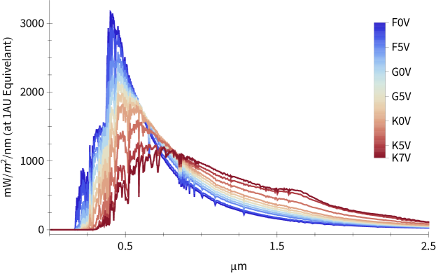
2.4 Initial Conditions
In our models, we keep the outgassing rates for H2, CH4, CO, N2O, and CH3Cl constant, and set the mixing ratios of O2 to 0.21 and CO2 to , with a varying N2 concentration that is used as a fill gas to reach the set surface pressure of the model (see also Segura et al., 2005, 2003; Rugheimer et al., 2013; Rugheimer et al., 2015b ; Rugheimer and Kaltenegger, 2018).Note that by keeping the outgassing rates constant, lower surface pressure atmosphere models initially have slightly higher mixing ratios of chemicals with constant outgassing ratios than higher surface pressure models. The dominant parameters we vary between simulations are the host star type and planetary surface albedo. Other parameters were altered slightly to aid in a more rapid convergence of the model, such as atmosphere height, and height of convection.
2.5 Albedos
The surface albedo in the 1D iterative climate-photochemistry code we updated for this study (Kasting and Ackerman, 1986; Kasting et al., 1979; Zahnle et al., 2006)
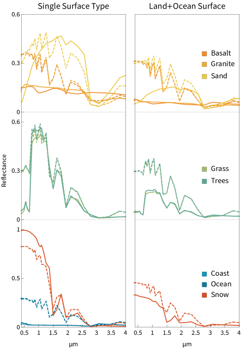
was a single value from 0.237m to 4.55m. To simulate Earth conditions for solar irradiation at Earth’s orbital position with a single albedo, a value of 0.31 is used for all wavelengths (e.g. Arney et al., 2016). To examine how different surfaces influence a planet’s climate, we updated the code to read in a wavelength-dependent albedo value.
Following Kaltenegger et al., (2007) we gathered surface albedos from the ASTER and USGS spectral libraries (Baldridge et al., 2009; Kokaly et al., 2017; Clark et al., 2007) to create an average present-day Earth surface albedo from 8 raw albedos of snow, water, coast, sand, trees, grass, basalt, and granite (Fig. 3.2). If the data was not complete in the UV, we extended the albedo constantly using the nearest value (these extensions affected regions smaller than 0.1 microns). For Earth clouds, we use the Modis 20m cloud albedo model (King et al., 1997; Rossow and Schiffer, 1999)(Fig. 3.3), which provides an average for many clouds of different droplet size. We then used this Earth surface albedo to determine what fractional addition of clouds results in the same surface temperature as the model using a flat albedo of 0.31. As discussed further in the results section, we find that using 44% cloud coverage in combination with the wavelength-dependent surface albedo of present-day Earth reproduces the same surface temperature and climate as the original albedo treatment of a single value of 0.31.
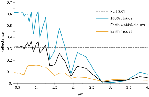
Note that the cloud fraction mimics the combined effect of warming and cooling due to clouds, which is why the fraction is lower than modern Earth’s actual cloud fraction, which is between 50% and 70% (Stubenrauch et al., 2013). Because of unknown cloud feedback for host stars with different SEDs, we then keep the cloud properties, reflectivity, and coverage constant to explore the influence of the surface albedo on the planet’s climate and spectra for different host stars.
3 Results
We model Earth-like planets with different surfaces for a representative grid of 12 host stars from F0 to K7 in approximately 350K effective surface temperature steps. Figures 3.4 and 3.5 show the temperature profiles along with the mixing ratio profiles of the major atmospheric chemicals of interest for characterization and biosignature detection H2O, O3, CH4, and N2O for planets with different surfaces with and without clouds. In this paper, we present the detailed temperature and chemical profiles of a select subset of 3 stars (K2V, G2V, F2V) and the spectra for a subset of 4 stars (K2V, G2V, F2V, F0V) in the figures for clarity.
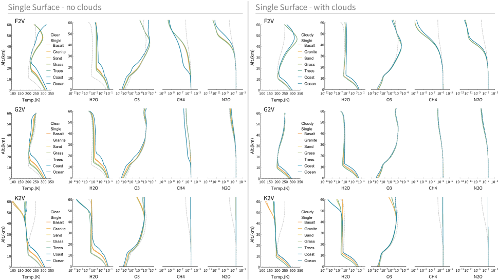
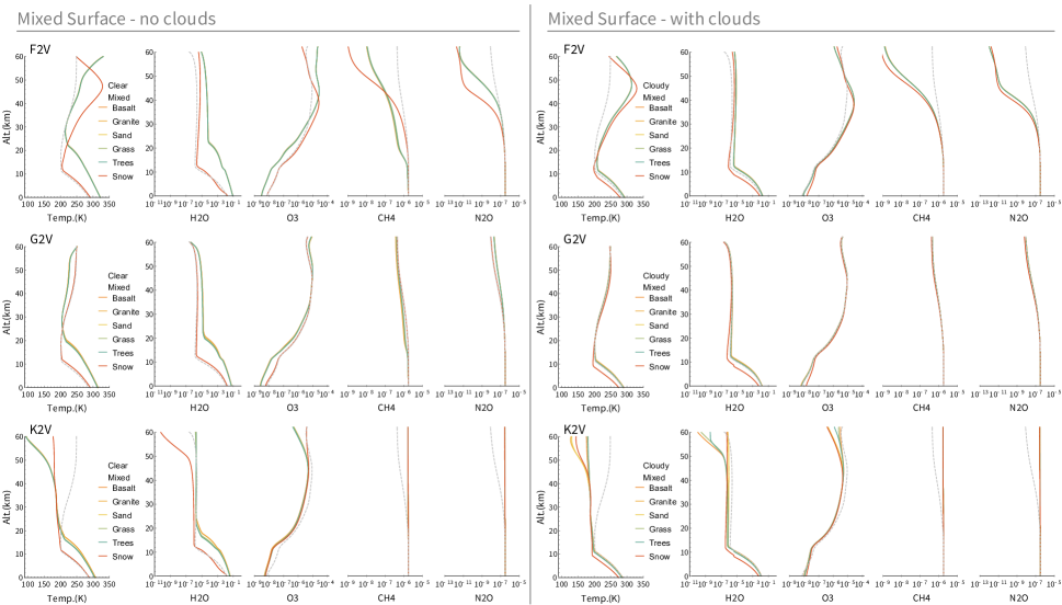
3.1 Surface Temperature for Earth-like Planets
Using our wavelength-dependent Earth surface albedo in combination with a 44% cloud fraction, we compare the results for our Earth-like planet models for each host star type to the flat albedo models. Fig. 3.6 shows that the deviation of the resulting surface temperature becomes larger as the stellar type becomes more different from the Sun. The wavelength-dependent Earth albedo is less reflective in the near IR than the flat albedo, which causes the planetary surface to become hotter around redder stars and cooler around bluer stars. For an Earth-analog surface, which the 1D flat albedo models were calibrated for, where the surface is dominated by 70% ocean, our results show that the wavelength dependence of the surface albedo increases the average surface temperature by up to 5K and decreases it by down to 1K (Fig. 3.6). However, the effects can be much stronger for planets that do not have modern Earth-analog mixed surfaces.
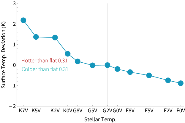
Our models show that planetary surface temperature generally increases with decreasing effective temperature of the host star, and temperature inversions in the upper atmosphere of the planet decrease (Fig.3.4 (see also Segura et al., 2007; Rugheimer et al., 2015a ). The absolute surface temperature generally is higher for clear atmosphere models as expected due to the high reflectivity of clouds. The surface temperature of ocean-worlds is higher due to the lower reflection of oceans compared to granite or basalt surfaces, which show higher surface temperatures than desert- and jungle-worlds.
While the trend of increasing surface temperature with decreasing host star effective temperature also holds for planets with similar surfaces, different surfaces can reduce the magnitude significantly e.g. an ocean-planet orbiting an F-star shows hotter surface temperature than a rocky planet orbiting a K-star (see Fig.3.4).
The chemical profiles in Figures 3.4 and 3.5 show an increase in methane and N2O concentrations as expected for host stars with lower surface temperatures, especially in the upper atmosphere (see also Segura et al., 2007; Rugheimer et al., 2015a ). The ozone concentration increases for host stars with lower surface temperatures as discussed in several papers (e.g. Segura et al., 2005, 2007; Rugheimer et al., 2015a ; Rugheimer et al., 2013).
3.2 Surface Temperature of Water-, to Desert-worlds around different host stars
To explore how the spectral type of the host star influences different kinds of potentially habitable worlds, we first model a planet covered entirely with a single surface, e.g. ocean covered water worlds (using the surface albedo of oceans), desert worlds (sand), jungle worlds (trees and grass) and rocky worlds (basalt and granite) with and without clouds. Since these single-surface planets have unique, non-flat surface albedos, their climates each respond differently to host stars with different SEDs. As a second step, we created a set of wavelength-dependent ocean-land surface models comprising of the wavelength-dependent albedo of one unique surface combined with 70% ocean coverage. Fig. 3.7 shows the average surface temperature differences between models assuming a flat 0.31 albedo and water-, jungle-, rocky- and desert-planets (top panel) and land-ocean surface coverage for clear and cloudy atmospheres (bottom panel). These results show that the surface of a planet can have a significant impact on the surface temperature of an exoplanet, and potentially alter habitability. For our single surface models, using a wavelength-dependent albedo instead of the constant albedo value changes the surface temperature for up to +35 K for an ocean planet orbiting an F0 host star and -10K for a cloudy jungle-planet orbiting a K7 host star (Fig. 3.7).
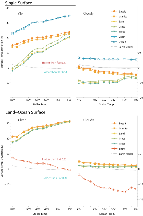
3.3 How Surfaces influence Spectra
We model the reflection spectra of Earth-like planets with different surfaces in the Habitable Zone to explore how different surfaces influence the spectra of potentially habitable worlds seen directly imaged.
Fig. 3.8 and Fig.3.9 show that some atmospheric species exhibit noticeable spectral features in reflected light (0.4 to 2m) as a result directly or indirectly from biological activity: the main ones are O2, O3, CH4, N2O and CH3Cl (see e.g. Des Marais et al., 2002; Kaltenegger, 2017). In the visible wavelength range, the strongest O2 feature is the saturated Frauenhofer A-band at 0.76m, with a weaker feature at 0.69m. O3 has a broad feature, the Chappuis band, which appears as a shallow triangular dip in the middle of the visible spectrum from about 0.45m to 0.74m. Methane at present terrestrial abundance (1.65ppm) has no significant visible absorption features, but at high abundance, it shows bands at 0.88m, and 1.04m, detectable e.g. in early Earth models (Kaltenegger et al., 2007; Rugheimer and Kaltenegger, 2018). In addition to biosignatures, H2O shows bands at 0.73m, 0.82m, 0.95m, and 1.14m. CO2 has negligible visible features at present abundance, but in a high CO2-atmosphere of 10% CO2, like in early Earth evolution stages, the weak 1.06m band could become detectable.
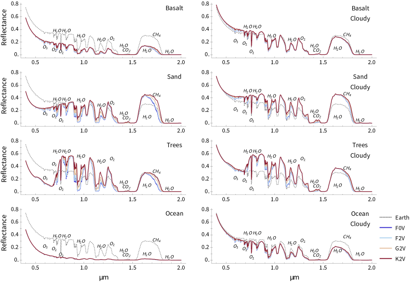
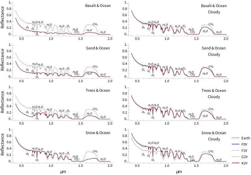
As discussed in detail in (Rugheimer et al., 2013; Rugheimer et al., 2015a ), features of Oxygen, water, Methane, and Carbon Dioxide are present in the visible/near IR spectrum. Aside from the dominant water features, the O2 feature near 0.76 m is clearly distinguished in the relative reflection around all model stars. Most features appear deeper for the models using the wavelength-dependent Earth albedo compared to the flat albedo. Note that the spectra have not been multiplied by the incident stellar flux, which will reduce the reflected flux in the shorter wavelength range significantly (see e.g. Rugheimer et al., 2015a ).
Along with the differences in surface temperature and photochemical differences described previously, the resulting reflectance spectra show changes between a wavelength-dependent Earth-analog surface model versus a flat albedo model (Fig. 3.10). This shows that assuming a flat albedo can both under- or over-estimate the strength of specific chemical atmospheric signatures for Earth-like planets, depending on their host stars.
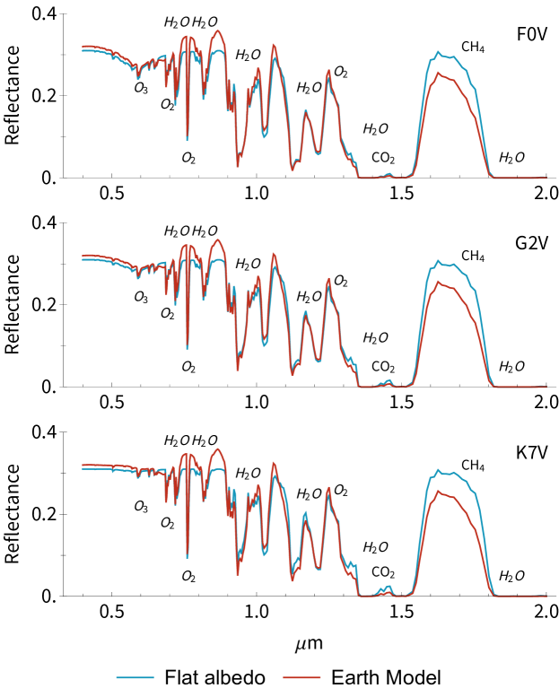
Since the wavelength-dependent Earth albedo reflects less than the flat albedo in the near IR, spectral features in the NIR will be overestimated if a flat albedo is used in an Earth spectrum model (Fig. 3.3).
Fig. 3.8 and Fig. 3.9 show relative reflectance for planet models with one surface as well as 30% land and 70% ocean coverage, respectively, for different host stars for clear (left) and cloudy (right) atmospheres. Note that the dashed line in both figures is the modern Earth reflection spectra, including clouds. Surfaces with lower albedo (e.g. water) reduce the reflected flux of the planet. In contrast, surfaces like sand and trees increase the overall reflectivity of a planet compared to modern Earth (dashed line).
The overall effect of the decreased stellar incident flux at shorter wavelengths for cooler stars makes atmospheric features like the 0.76m O2 challenging to detect for cooler stars (see also e.g. Rugheimer et al., 2015a ). However, the shape of the surface albedo (e.g. sand reflection increases with decreasing wavelength compared to modern Earth) can increase and decrease the detectability of specific atmospheric features.
For atmospheric models, including clouds, the overall reflectivity of the planet increases due to the added high cloud albedo. However, the overall results from the single surface planet models discussed above hold, even though the coverage of the surface reduces due to the added 44% cloud coverage in the planet models.
Earth‘s surface consists of about 70% ocean and 30% land. Therefore we also model this specific case to provide a second comparison set. Assuming one single surface dominates the remaining landmass (basalt, sand, trees, or snow), we explore the effect on the reflection spectra of such planets. Note that the 100% ocean covered surface has been shown in Fig. 3.8. Adding 70% ocean reduces the overall reflectivity of the planet because oceans only reflect a small amount of incident light (Fig. 3.2). While the overall reflected flux reduces for all models (Fig. 3.9), the overall signature changes discussed above hold for the land-ocean models as well under both clear and cloudy conditions.
The spectra shown in Fig.3.8 and Fig.3.9 show that increasing cloud coverage and decreasing surface coverage of individual surfaces decrease the detectable differences in reflected flux for planets with different surfaces (as discussed in Kaltenegger et al., (2007).
Several teams has discussed observations of Earth-size planets in the habitable zone with upcoming extremely large telescopes (see e.g. Kaltenegger and Traub, 2009; Kaltenegger et al., 2010; Stevenson et al., 2016; Barstow and Irwin, 2016; Hedelt et al., 2013; García Muñoz et al., 2012; Snellen et al., 2013; Rodler and López-Morales, 2014; Bétrémieux and Kaltenegger, 2014; Misra et al., 2014). Different surfaces of planets can influence the overall abundance of chemicals in the atmosphere, via their influence on the surface temperature of a planet and the resulting photochemical changes. Note that these changes affect most spectral lines (especially water, oxygen, and methane).
4 Discussion
4.1 Single surface models explore the most extreme effect
Our exploration of the influence of the surface on an exoplanet‘s climate and spectra shows the most extreme effect for planets fully covered with a single surface (Fig. 3.8). We chose this case to explore whether wavelength-dependent surfaces affected the climate and surface temperature of exoplanet models. In addition to the most extreme case, a single surface coverage, we also show a second comparison set in this paper, analog to Earth, we assume a 70% ocean coverage of the planet‘s surface. While the fraction of different surfaces on exoplanets in unknown, these two cases show i) the maximum effect of a surface on a planet‘s climate as well as ii) the reduced effect if only 30% of a planet‘s surface is covered with a specific surface. While many other options are possible, these two cases clearly show how the surface fraction, as well as clouds, influence the climate of Earth-like planets. Any other surface fraction can be interpolated from the cases shown. While we do not know what surfaces exist on Earth-like exoplanets, We chose the 8 dominant surfaces of our own planet here as the test cases in our models (Fig. 3.3). In an exoplanet context, the interaction of wavelength-dependent surface albedo and stellar spectra has been examined mainly regarding the effect of ice-albedo feedback or special case surfaces (Abe et al., 2011; Shields et al., 2013, 2014; Shields and Carns, 2018). Some of our cases resembled those previously studied with snow/ice surfaces, which we confirmed show increased heating for planets around K-stars compared to G- and F-stars.
4.2 Cloud feedback is unknown for different host stars
Cloud feedback is unknown for different host stars. We, therefore, use clouds with similar properties for all our models based on the modern Earth model, as explained in section 2 as a first-order approximation. Cloud properties and coverage depend on many factors, including planetary rotation rate, atmospheric pressure, temperature, aerosol abundance, particle size distribution, and humidity (see e.g. Zsom et al., 2012). Cloud coverage on Earth changes seasonally and is thought to have also changed over geologic time (see e.g. O’Malley-James and Kaltenegger, 2018b ; Brierley et al., 2009).
4.3 3D and 1D model exploration of rocky planets
3D models are being expanded to explore rocky exoplanets, with a large body of papers advancing a lively discussion in the literature on how to best include the feedback effects of clouds, rotation, surface features, atmospheric dynamics, and full photochemistry in 3D models (see e.g. discussions in Gomez-Leal et al., (2016, 2019); Forget and Pierrehumbert, (1997); Chen et al., (2019); Lorenz et al., (1997); Williams and Pollard, (2002); Joshi, (2003); Lopez et al., (2005); Selsis et al., (2007); Edson et al., (2011); Zsom et al., (2012); Goldblatt et al., (2013); Leconte et al., 2013b ; Leconte et al., 2013a ; Leconte et al., (2015); Vladilo et al., (2013); Wordsworth and Pierrehumbert, (2013); Yang et al., (2013); Boschi et al., (2013); Ferreira et al., (2014); Wolf and Toon, (2015); Linsenmeier et al., (2015); Kopparapu et al., (2016); Popp et al., (2016); Kitzmann, (2017).) 3D models and 1D models tend to be in agreement on globally averaged surface temperature for a range of stellar types though some 3D effects can exacerbate this difference due to cloud feedback Arney et al., (2016), tidal locking Kopparapu et al., (2016), or at climate extremes such as habitable zone edges Shields et al., (2013); Yang et al., (2016); Gomez-Leal et al., (2019).
Our 1D model includes detailed photochemistry based on Earth’s atmosphere and is, therefore, an excellent tool to explore the effect of the host’s SED and the wavelength-dependent surfaces on the changes in the atmosphere of Earth-like planets orbiting different host stars. We concentrate on F, G, and K stars in this paper, where rocky planets in the HZ should not be synchronously locked to their host stars, and thus effective heat transfer in an Earth-like atmosphere can be assumed (see e.g. Joshi, 2003). We use a 1D model for this study to explore a large range of surfaces and star types.
5 Conclusions
Our paper demonstrates the importance of including the wavelength-dependent feedback between a planet’s surface and a planet’s host star for Earth-like planets in the HZ of stars with an effective temperature between 3,900 and 7,400 K, corresponding to K7V to F0V main sequence stars. The heating or cooling effect of a specific surface is due to the interplay between the host star’s SED compared to the shape of the wavelength-dependent surface albedo and can substantially change the surface temperature of an Earth-like planet. Our paper demonstrates the importance of including the wavelength-dependent feedback between a planet’s surface and a planet’s host star for Earth-like planets in the habitable zone. Reflected light from the surface plays a significant role not only on the overall climate but also on the detectable spectra of Earth-like planets.
Data Access
DOI for accompanying data: 10.5281/zenodo.3912065
Acknowledgements
This work was supported by the Brinson Foundation and the Carl Sagan Institute. We would like to thank Zifan Lin, Thea Kozakis, and Sarah Rugheimer for comments and insights.
![[Uncaptioned image]](/html/2010.05046/assets/art/MFA_d4.jpg)
Chapter 4 Ready Student One: Exploring the predictors of student learning in virtual reality
This thesis chapter originally appeared in the literature as
J. Madden, S. Pandita, J. P. Schuldt, B. Kim, A. S. Won, and N. G. Holmes, PLOS ONE 15(3): e0229788 (2020)
1 Abstract
Immersive virtual reality (VR) has enormous potential for education, but classroom resources are limited. Thus, it is important to identify whether and when VR provides sufficient advantages over other modes of learning to justify its deployment. In a between-subjects experiment, we compared three methods of teaching Moon phases (a hands-on activity, VR, and a desktop simulation) and measured student improvement on existing learning and attitudinal measures. While a substantial majority of students preferred the VR experience, we found no significant differences in learning between conditions. However, we found differences between conditions based on gender, which was highly correlated with experience with video games. These differences may indicate certain groups have an advantage in the VR setting.
2 Introduction
In twenty-first century education, technology is pervasive in our classrooms (Maddux, 2003). Research has found many ways in which technology benefits student learning and attitudes towards science (Singer et al., 2012). As new instructional technologies are developed, it is necessary that researchers conduct critical evaluations of their effectiveness. There are many open research questions related to identifying how to most effectively use different kinds of technology for different learning goals or for different points in the learning process. One technology that has received particular attention for its potential in science learning is virtual reality and other immersive media (Dede, 2009; Pan et al., 2006).
In a typical college lecture for a science course, an instructor can choose to engage students with a concept using technologies such as specialized equipment for an interactive lecture demonstration (Sokoloff and Thornton, 1997), a dynamic computer simulation (Wieman et al., 2008), or classroom polling with personal response systems (Stains et al., 2018). Science courses also employ technology extensively in instructional labs, where students can use technology to obtain first-hand experiences with the phenomenon (Hofstein and Lunetta, 2004). Instructional labs, however, have failed to provide measurable gains in student learning of those phenomena (Holmes et al., 2017; Etkina et al., 2010), reminding us that what is important for learning is not the technology itself, but how and why it is used (Singer et al., 2012). For example, using relatively similar equipment, interactive lecture demonstrations have consistently found measurable learning gains when students are actively engaged in making predictions and explaining the observations from the demonstrations (Sokoloff and Thornton, 1997; Crouch et al., 2004). Interactive simulations have also been shown to improve or replicate learning compared to hands-on manipulatives, while reducing the associated resources (Finkelstein et al., 2005; Chini et al., 2012). While there are many potential explanations for these differences (Smith and Holmes, 2017), two relate to how learners and technology interact through issues of embodiment and real-world complexities. This study aimed to test the impact of these variables by directly comparing student learning and attitudes from three different instructional technologies (a hands-on activity, desktop simulation, and virtual reality simulation), while taking advantage of their respective affordances along the dimensions of embodiment and real-world complexity.
2.1 Embodiment
Theories of learning argue that cognition is inherently embodied: “the mind must be understood in the context of its relationship to a physical body that interacts with the world.” (Wilson, 2002, p.625). Research has found that learning benefits from activities that explicitly attend to embodied cognition (Anderson, 2003; Roth and Jornet, 2013; Carbonneau et al., 2013). There are several ways in which embodiment is argued to support learning, generally tied to a hypothesis whereby activities help move cognition from abstract to concrete representations of a phenomenon (Anderson, 2003).
Two such notions of embodied cognition focus on how learners off-load cognitive work on to the environment and how off-line cognition is body-based (Wilson, 2002; Martin and Schwartz, 2005). These notions suggest physical aspects of cognition, whereby learning is supported through engaging perceptuo-motor systems (Tsang et al., 2015). Indeed, nearly all science education advocates for the use of interactive hands-on activities (Ruby, 2001). Through hands-on activities and demonstrations, learners connect abstract concepts to their physical environment. For example, researchers in physics education have developed embodied activities for teaching concepts of energy conservation (Scherr et al., 2013). In these activities, learners assign units of energy to physical objects (either cubes or people) (Scherr et al., 2012), and then manipulate those objects to represent processes of energy transfer and dynamics. Through these concrete representations of an otherwise abstract phenomenon, learners develop their conceptual and mechanistic understandings of the phenomenon (Scherr et al., 2013). By manipulating physical objects, students can see deep features of the phenomena, allowing them to effectively integrate the features into their mental models of the phenomena (Tsang et al., 2015; Piaget, 2013).
Two other notions of embodied cognition focus on how cognition is situated within the real-world and that the learning environment is part of the cognitive system (Wilson, 2002; Martin and Schwartz, 2005). Because the knowledge learned is tied to the environment in which it was learned, it is argued that there are limitations to applying the knowledge in new environments (Brown et al., 1989). In science education, the initial learning environment can often seem too far removed or distinct from the intended environment for applying the knowledge. Context-rich activities, can provide concrete, real-world scenarios for otherwise abstract learning activities. Alternatively, activities may be modified to better represent the real world, such as by providing realistic representations of the phenomena.
These activities also demonstrate that there are degrees of embodiment. These may range from metaphorical groundings of cognition (for example, being able to imagine oneself walking from point A to point B) to physically experiencing the phenomenon (for example, actually walking from A to point B) (Anderson, 2003). While much research has demonstrated the benefits of physically experiencing the phenomenon through hands-on activities, the results are not universal (Cunningham, 1946; Holmes et al., 2017; Chini et al., 2012; Finkelstein et al., 2005; Klahr et al., 2007). One explanation for the lack of clear benefit for hands-on activities is that when the activities and materials are complicated or difficult to manipulate, the learner may experience extraneous cognitive load (Paas et al., 2003) or may be likely to make mistakes (Sokoloff and Thornton, 1997). That is, real-world complexity gets in the way of student learning in hands-on activities.
2.2 Real-world complexity
In a real-world experiment, students’ measurements and observations are prone to variability, systematic effects, and measurement mistakes that are not relevant to the theoretical concepts being taught. In general, people struggle to evaluate uncertain events (Kahneman and Tversky, 1972) and use error-prone shortcuts and heuristics in making judgments under uncertainty (Tversky and Kahneman, 1974). Learning an underlying concept, then, becomes difficult if the information being used to develop that understanding is uncertain or probabilistic.
For hands-on activities, the uncertain and probabilistic elements contribute to extraneous cognitive load during the activity. Cognitive load refers to a learner’s capacity for processing information in their short-term memory (Paas et al., 2003). Information can either contribute to extraneous (ineffective) cognitive load or germane (effective) cognitive load (Paas et al., 2003). Germane cognitive load refers to information that is relevant for learning, such that large amounts of germane cognitive load can improve learning (Kapur, 2016). Extraneous cognitive load refers to information that is irrelevant for learning, such that large amounts of extraneous cognitive load impede learning (Sweller and Chandler, 1991; Paas et al., 2003). In hands-on activities, issues of uncertainty, complicated equipment, and user mistakes contribute to extraneous cognitive load, which may hamper learning.
To reduce that cognitive load, hands-on activities often use heavily guided instructions that attempt to limit mistakes, tell students how to manipulate the equipment, and reduce uncertainties (Hofstein and Lunetta, 2004). However, constructivist theories of learning argue that students must have the ability to explore and generate their own knowledge (Bransford et al., 1999). The key is to develop activities with high germane cognitive load, but low extraneous cognitive load (Kapur, 2016; Schwartz et al., 2011).
Simulations are one way to remove the extraneous cognitive load of real-world hands-on activities, allowing phenomena to be demonstrated in a consistent and controlled way. With that control, they can still be relatively unstructured, maintaining high germane cognitive load. Students can autonomously and easily change variables, allowing them to learn at their own pace (Price et al., 2018; Podolefsky et al., 2010). Several studies have found that computer simulations produce equal (Darrah et al., 2014; Chini et al., 2012; Evangelou and Kotsis, 2018) or better (Finkelstein et al., 2005; Chini et al., 2012) learning than hands-on activities. Simulations also provide opportunities for students to see features of a phenomenon that they would be unable to see otherwise, for example abstract concepts such as heat (Strzys et al., 2018) or microscopic objects such as cells (Chang et al., 2016) or electrons (Finkelstein et al., 2005; Kapp et al., 2019).
Simulations, however, provide a more limited embodied cognition experience than hands-on activities, where the learner interacts directly with the phenomenon. Virtual reality is a potential technology that can employ high-levels of embodiment, while maintaining controlled and simplified representations of the phenomena to be learned.
2.3 Why virtual reality?
Immersive virtual reality (VR) may provide the best of both worlds. VR allows embodied simulations and offers a number of other affordances (Bricken, 1991; Perone, 2016) that make it uniquely suited as a teaching tool for basic science. First, students can physically interact with content, providing the engagement of a hands-on activity but with the control and replicability of a simulation. Second, the simulations provide multiple forms of embodiment, such as changing perspectives to experience phenomena as they would in different circumstances in the real world (Anderson, 2003). Third, students can experience these perspectives in ways unavailable in the real world (Price et al., 2018; Strzys et al., 2018; Kapp et al., 2019). From a research perspective, the ability to track student movement allows for assessing engagement and learning (Won et al., 2014) to better test the embodiment hypothesis. It also facilitates implementing interventions to increase learning in real time.
There is thus a need for experimental research that directly tests the effectiveness of VR on science learning, over-and-above that offered by existing hands-on and simulation approaches. Several studies have compared learning between these three modalities and found that, in terms of student attitudes, participants generally prefer learning in VR over other modalities (Smith et al., 2017; Chang et al., 2016). One study even found that students’ attitudes towards socio-scientific issues improved more in an augmented reality (AR) simulation over a desktop simulation, even though these aspects were secondary to the activity’s primary cognitive goal (Chang et al., 2016). Related to embodiment, several studies have found that participants became more immersed in VR than in other environments (Lier et al., 2018; Makransky et al., 2017; Winn et al., 2002). Generally, this immersion seems to be independent of personal characteristics, such as gender, VR experience, and time spent gaming (Lier et al., 2018).
Measures of learning from VR are generally conflicting. Studies have found that participants in VR learn more than (Winn et al., 2002; Strzys et al., 2018), as much as (Smith et al., 2017; Chang et al., 2016), or less than (Makransky et al., 2017) participants in hands-on or desktop conditions. When learning was improved in VR over a hands-on activity, the gains were attributed to immediate feedback available through the simulation and visualization of the abstract phenomenon that was otherwise imperceptible in the hands-on activity (Strzys et al., 2018). When learning was hindered in VR over a desktop simulation, the differences were attributed to higher cognitive load (Makransky et al., 2017). In this study, where participants answered multiple-choice questions and performed technical lab procedures in the two types of simulation, researchers found that students in the desktop simulation condition learned more than students in the VR condition on a conceptual test. However, learning was the same between conditions on a transfer test and participants overwhelmingly preferred the VR condition. The researchers also found that participants in the VR condition had significantly higher cognitive load as measured through an electroencephalogram (EEG). They suggested that the physical manipulation of the equipment in VR was more complicated than the desktop condition, which may have increased students’ extraneous cognitive load, impacting learning. They recommended experiments that used more natural control systems to manipulate the environment. Furthermore, the researchers also argued that the enjoyment associated with VR actually distracted the learners from learning.
In addition to cognitive load, there are also questions about gender differences and experience with 3D rotations through experience with video games. In one study, men outperformed women during the task itself, but there was no difference on a post-condition recall test (León et al., 2018). In a study that found no overall differences in learning from VR compared with video and static images, the researchers found that men and participants with experience with video games outperformed in the VR condition over other conditions and participants (Smith et al., 2017). Because gender was also correlated with video game experience, they hypothesized that video game experience was a proxy for the gender differences emerging in their study. This result is somewhat surprising given that neither condition involved much interaction with the simulations (even the VR participants could only look around the simulation).
Research has found, however, that performance is improved when participants can more fully interact with the simulation: for example, walking around the simulation compared with remaining stationary while looking around the simulation (León et al., 2018). Furthermore, one study found that students’ reported sense of presence in a simulation was correlated with their learning from the simulation (Winn et al., 2002). This study also found that preferential learning from VR was confined to sub-topics involving “dynamic three-dimensional processes, but not processes that can be represented statically in two dimensions” (Winn et al., 2002, p.1). This suggests that VR simulations are more effective when they take advantage of their specific affordances.
The existing research exemplifies the idea that it is not the technology, but how it is used, that promotes learning. In this study, we aimed to develop and test a VR simulation that took advantage of its various affordances, particularly related to embodiment and real-world complexity. We probed these ideas by comparing an interactive VR condition with analogous hands-on and desktop simulation activities for learning about Moon Phases. As per the previous research, we evaluated students’ conceptual knowledge, long-term retention, attitudes towards the activity, and socio-scientific beliefs. We also compared differential effects on sub-populations of our participants, including evaluating effects for gender, video game experience, and experience in VR. We found that there were no overall differences in learning on short-term or long-term assessments between conditions and that the immersive VR did not impact students’ socio-scientific beliefs. We also replicated previous work in that participants overwhelmingly preferred the VR condition, and that men outperform in the VR condition, which may be attributed to video game experience.
3 Methods and Materials
This study had two hypotheses. First, we proposed that there would be a main effect of virtual reality on learning. Second, we proposed that there would be corresponding effects on environmental attitude. We also collected data on other measures in order to explore interactions that might be predicted by the literature. All measures are reported below.
In our study, we used a between-subjects pre-post design, with three conditions. The three conditions were designed to express the same content using different educational tools; an immersive simulation using a VR headset, a computer-based interactive desktop simulation, and an analog hands-on activity (Fig. 4.1). We chose the concept of Moon phases, as it was expected to benefit from embodiment and reduction of real-world complexities. A review of over 35 years of astronomy education literature found that phases of the Moon was one of the most challenging topics in astronomy education (Lelliott and Rollnick, 2010). A lesson on Moon phases requires the student to place themselves in spatial and temporal perspectives of the Sun-Earth-Moon system that are generally inaccessible, which can be challenging through static images or text (Galano et al., 2018; Türk and Kalkan, 2015). Previous work has found that students’ spatial reasoning correlates with their understanding of lunar concepts (Wilhelm et al., 2013; Cole et al., 2018). Understanding of Moon phases also requires understanding the dynamic evolution of the phases over time and space (Cole et al., 2018), likely facilitated through interacting with and moving around a simulation. Furthermore, the traditional hands-on activity for teaching Moon phases (described below) is susceptible to various real-world inaccuracies, such as creating eclipses every month or rotating or orbiting the wrong way. Research has also found that explanatory features of traditional descriptions and images can interfere with student understanding (Galano et al., 2018; Türk and Kalkan, 2015), motivating the need for authentic real-world visualizations over abstracted ones.
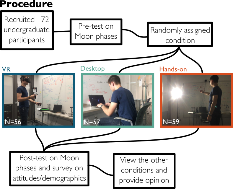
3.1 Participants
Participants were recruited from the undergraduate student population of a medium-sized private university. There were 172 participants, including 138 women, 31 men, and 3 other, all between the ages of 18 and 24. For three conditions to obtain a Cohen’s d effect size of 0.25 with 80% statistical power at 95% significance level, our power test determined that a sample size of 53 participants per condition (159 total) would be sufficient. We ran a total of 172 participants to buffer against potential exclusions. The study primarily drew from students currently enrolled in an introductory astronomy class (varying in major), and students majoring in Communication. Participants’ self-reported race and ethnicity were as follows: 62 Asian/Pacific Islander, 59 Caucasian, 21 African American, 18 bi/multiracial (including Asian/Pacific Islander, Caucasian, African American, Hispanic/Latinx, and Native American), 6 Hispanic/Latinx, 4 preferred not to answer, and 2 specified ‘other’ without elaboration. Participants could select as many categories that applied. All participants signed an informed-consent form before beginning the experiment. All aspects of the experiment were approved by the Cornell Institutional Review Board Protocol #1708007381. Participants were compensated with course credit or 15 dollars in cash for their participation. The individual pictured in Fig. 4.1 has provided written informed consent (as outlined in the PLOS consent form) to publish their image alongside the manuscript.
Participants first took a pre-test and then they were randomly assigned to one of three conditions. After the activity (which included consistent self-guided lessons on Moon phases, described below), participants took a post-test that included a demographic and attitudinal survey. Finally, the participants were shown the other two conditions and asked to comment on which they would prefer as their favorite learning method and why. These activities are summarized in Fig. 4.1. A large preference for one condition over another may lead to greater retention of knowledge learned in that condition. To explore this potential effect we contacted all participants four months after participating and asked them to complete another learning test (delayed post-test). We received 56 responses to the delayed post-test making a breakdown by demographics difficult.
3.2 Conditions
Each condition was designed to give participants a similar learning experience using the three technologies we employed. The overall design was to recreate a Sun-Earth-Moon system that the participant could control in time in order to observe the changes in the Moon’s phase and the positions of the Sun, Earth, and Moon during each phase. In each condition the participant could move forward and backward in time and had control over the perspective from which the system was being viewed. Each condition also contained guiding questions for the participant to assist with navigating and learning from the simulation.
VR Simulation
The VR simulation was designed to mimic the hands-on activity as closely as possible, while still taking advantages of the technology’s unique affordances. In the VR simulation, participants used a headset and controllers that tracked their motion and rendered the environment, providing an immersive and interactive experience (Fig. 4.1, left). The simulation contained a realistic Sun-Earth-Moon system in which the participant had control over time and their viewing location (Fig. 4.2). Students could control the Moon phases by moving forwards and backwards in time with simple button presses or grabbing the Moon to move it in its orbit. Upon entering the simulation, participants were initially placed on top of the Earth’s north pole, but they could change their position to be far above the Earth to provide a more diagrammatic view of the system or to be near the surface of the Earth to view a realistic horizon as the Sun or Moon rises and sets. The participants were given the guiding questions throughout the experience via a virtual clipboard attached to their hand to help students interact with and learn from the environment. The names of the Moon phases were displayed in the environment as the participant moved the Moon. The simulation was created by our team using the Unity game engine for use with the Oculus Rift VR headset.
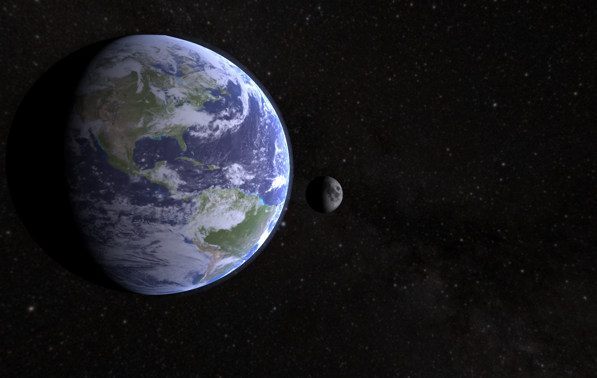
Desktop Simulation
The desktop simulation was designed to mimic the VR activity as closely as possible. In the desktop simulation, participants were shown a realistic Sun-Earth-Moon system on a laptop with controls over the camera position and time (Fig. 4.1, middle). The environment was created using the same system as the VR simulation (Fig. 4.2). Participants could control the Moon phases by going forwards and backwards in time through arrow key presses. They could also navigate around the environment using the mouse and scroll to zoom. The participants were given the guiding questions using a tablet device outside of the simulated environment. The names of the Moon phases were displayed in the environment as the participant moved the Moon. This simulation was created by our team using the Unity game engine.
Hands-on activity
The hands-on activity was based on traditional classroom activities about Moon phases (Newbury, 2011). In this activity, the participant’s head represented the Earth; the Moon was represented by a small ball held at arm’s length; and the Sun was represented by a stationary light (Fig. 4.1, right). Participants were asked to rotate counter-clockwise to observe changes in the Moon’s phase, as observed in the shadowed portion of the ball’s surface. Through this action, real-world complexities arise where the phenomenon may be inaccurately presented. For example, due to the relative distances and sizes between the ball and the participant’s head, participants may see eclipses every month. Subtleties such as inclination and procession of the orbits are uncontrollable and missed in the hands-on activity. The participants were given the guiding questions using a tablet as well as the names of the Moon phases.
3.3 Measures
To evaluate the effects of the different conditions, we assessed student understanding of Moon phases using existing pre-post assessment instruments, their attitudes towards the activities and the environment, and tracked their movements in the simulations.
Moon phases assessment
The pre- and post-tests each consisted of 14 multiple choice questions about Moon phases and the Moon’s motion relative to the Earth, sourced from existing research-validated assessments (Hufnagel, 2002; Lindell and Olsen, 2002; Lindell, 2004; Slater, 2014). The selected items included ones where the activities were both likely (orbit direction and period) and unlikely (rise and set times) to impact learning. Because the time between the pre- and post-tests were so short, the questions on each test were isomorphic and matched on content, but not identical. The delayed post-test questions were similar to the ones found on the post-test. On all tests, each question had only one correct answer, and the participant’s score was the sum of the number of correct answers, with all questions weighted equally. The item-test correlation and item difficulty turned out to be 0.37 and 0.34 for the pre-test and 0.43 and 0.59 for the post-test respectively based on all participant scores.
We also examined learning across conditions on each sub-topic on the assessments by comparing performance on the isomorphic questions. One of the deciding factors in choosing a certain technology as an educational tool is the affordances it offers to teach different aspects of the lesson. For learning about Moon phases, for example, the orbit and rotation periods are not controlled in the hands-on condition, but are constrained to be realistic in the desktop and VR simulations. Keeping the Moon’s orbit fixed is a task the participants must preform in the hands-on condition that does not require conscious effort in the other conditions. Differences between the technologies to control or not control certain aspects of the activities, therefore, may lead to differences in participant performance on knowledge questions in different topic areas despite showing the same performance between conditions on the whole exam. Our test contained a question pair that, upon investigation, was not truly the same from pre-test to post-test. Though they referred to the same general topic of why phases occur, they were not isomorphic and the question pair was removed from our analysis. The removal of this question did not significantly alter the results of our analysis.
Demographic survey
The demographic survey was provided at the end of the post-test and asked about a variety of participants’ characteristics.
Gender: Participants were asked their gender with the choices of Male, Female, or Other. For the analysis involving gender as a variable we removed the three participants who chose Other, due to low sample size.
Video game Experience: Participants were asked “On average, how frequently have you played video games over the past three years?” and the choices were daily, weekly, 1-2 times a month, 1-2 times a year, or never. We grouped the choices of daily, weekly, and 1-2 times a month into the category of ‘having significant video game experience’ and the participants who chose 1-2 times a year or never as ‘not having significant video game experience.’
VR experience: Participants were asked “How much virtual reality experience did you have before you participated in the experiment today?” and the choices were very minimum, moderate, a lot, or none. We grouped the participants who specified moderate or a lot as ‘having significant VR experience’ and the other participants as ‘not having significant VR experience’. Only one participant indicated having a lot of VR experience. We maintained three categories of VR experience: none, minimal VR experience, and moderate to high VR experience.
Academic Major: Participants were asked to pick their academic major from a list or write their own. For our analysis we grouped participants according to whether their major was science-focused or non-science-focused. Non-science majors included arts, humanities, economics, social science, communication, and business. Science majors included physics, astronomy, engineering, biology, chemistry, computer science, information science, and math.
Environmental attitudes survey
We also added an exploratory set of questions to probe participants’ socio-scientific attitudes through measurements of their individual differences in environmental attitudes using 15-items selected from the Environmental Attitude Inventory (EAI) (Milfont and Duckitt, 2010; Dunlap et al., 2000). We suspected that participants in our VR activity might come out with different socio-scientific attitudes, based on similar outcomes found in previous work (Chang et al., 2016; Ahn et al., 2016). In our simulation, we wanted to test the possibility that viewing the planet from the unique vantage point of space (an astronaut-like perspective of the Earth) might have an impact on environmental consciousness (Dunlap and Liere, 2008; Poole, 2010; Stepanova et al., 2019). This effect is attributed to a recognition of the the planet’s limited resources (Dunlap and Van Liere, 1978). Specifically, we selected five questions corresponding to each of three of the EAI’s subscales of particular interest to test whether the intervention influenced participants’ environmental movement activism, environmental threat, and human utilization of nature. Sample items were “I would not want to donate money to support an environmentalist cause,” “When humans interfere with nature it often produces disastrous consequences (R)” and “In order to protect the environment, we need economic growth” (1 = Strongly agree to 7 = Strongly disagree), and the modified scale showed sufficiently reliability (Cronbach’s ).
Activity preference
After completing the post-test, demographic questions, and EAI, participants were invited to try the other two conditions. They then completed a short survey that asked, “Today, you have experienced three different ways of learning moon phases. Which of the three ways to simulate the moon phases is your favorite method?” Participants could select either “Demonstration in virtual reality,” “Hands-on demonstration,” or “On-screen demonstration.” They were then asked, “Please briefly explain, why did you prefer this learning method?” with an open text box answer.
Virtual Reality Only Analyses
Analyses on presence and movement measures will be included in a subsequent publication, as only those in the virtual reality condition answered these questions or had head and hand movements, specifically, tracked.
Presence: Fourteen questions from two presence questionnaires (Aymerich-Franch et al., 2012; Witmer and Singer, 1998) measured participants’ sense of spatial presence in the virtual reality activity. Questions drawn from these surveys involved asking participants how much they agreed with the following statements: “I was really in outer space,” “I felt surrounded by outer space,” “I really visited outer space,” and “The outer space seemed real.” The participants assigned to the VR condition were also asked if they had experienced any simulator sickness during the activity and if it was distracting.
Movement tracking and controller use: The X, Y, and Z position and the pitch, yaw, and roll rotation of participants’ head and hands were recorded for the entire session in the VR condition. Movement from timepoint to timepoint may be calculated as the Euclidean distance (mm) between the positions of a tracker at time one and time two. Because the current paper focuses on the comparisons between the three conditions, analysis of the VR specific data, which includes movement, button presses, and presence measures, will be presented in a subsequent publication focused only on participants’ experiences in the VR simulation.
3.4 Data analysis
After all of the data had been collected we cleaned the data set by merging the survey results and verifying participant responses. The full data set was checked for inaccuracies, duplicates, and was translated into the proper form for analysis. Mathematica and R (R Core Team, 2017) packages were used for the analyses. All data and code are available through the CISER data archive (ciser.cornell.edu/data/data-archive/)
First, performance on the pre-test, post-test, and delayed post-test were compared between conditions using Analysis of Variance. Effects of condition on environmental attitudes were compared between conditions using ANOVA. Linear regression analyses were used to evaluate effects of other variables on student performance on the post-test, controlling for pre-test score. Variables were selected based on prior literature and included condition, gender, video game experience, and VR experience. Variables were checked for correlation using the ggpairs function from the GGally package in R, recording each variable level as numeric. The only significant correlation was between gender and video game experience, with a correlation coefficient of 0.47. Gender and video game experience were, therefore, analyzed separately in all regression analyses. Variance Inflation Factors (VIF) were also calculated in all regression analyses to measure possible collinearity. Main effects were tested first without interactions, and then regressions with interactions between condition and video game experience, gender, and VR experience were tested next. For the regression analyses, the base variables were a female, non-science major in the hands-on condition, with no VR experience, and not having significant video game experience.
4 Results
We describe our results grouped by overall differences in learning and attitudes based on condition and then by interactions between other variables.
4.1 Overall learning between conditions
The average score on the pre-test was 33.7% with no significant differences between the three conditions: F(2,169)=1.04, . Student performance significantly increased from pre- to post-test by 25.3% on average (average score of 59.1%), with no significant differences between the post-test scores across the three conditions: F(2,169)=0.815, (Fig. 4.3). An ANCOVA controlling for pre-score also showed no differences between the post-score between conditions: F(2,168)=1.07, . The average score on the delayed post-test(completed approximately four months after participation in the activity) was 39.0%, again with no differences between conditions: F(2,51)=0.571, . Our overall normalized gain of 0.38 is similar to that reported in an experiment involving pre-post moon phase assessments for a 20 minute inquiry-based tutorial of 0.54 (Lindell, 2004).
Our pre and post tests were not designed to be unidimensional and therefore did not reach a high Cronbach’s alpha ( for pre test, for post test). This is expected for multidimensional multiple choice tests (Wilcox and Pollock, 2014; Cortina, 1993). Both of our tests gave scores across a sufficient range according to Ferguson’s delta ( for pre test, for post test).
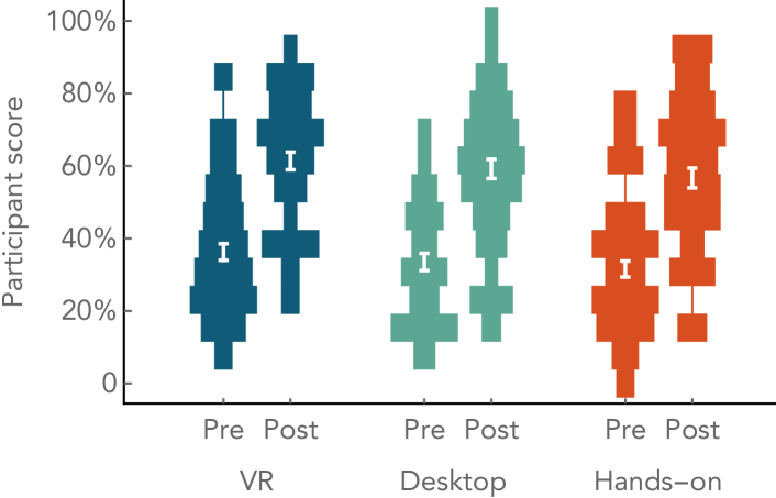
4.2 Learning by question
Breaking down the pre- and post-test scores by question show consistent gains between conditions, with no statistically significant differences (Fig. 4.4). Across the conditions, some topic areas showed large gains over 40% (orbit period, phase period, and illumination), while others showed small gains less than 10% (scale, Moon rotation, phase diagram, rise/set time), consistent with previous research on learning about Moon phases (Lindell, 2004; Wilhelm et al., 2018). This demonstrates that learning did not differ between conditions on sub-topics that may have held learning benefits within the different conditions.
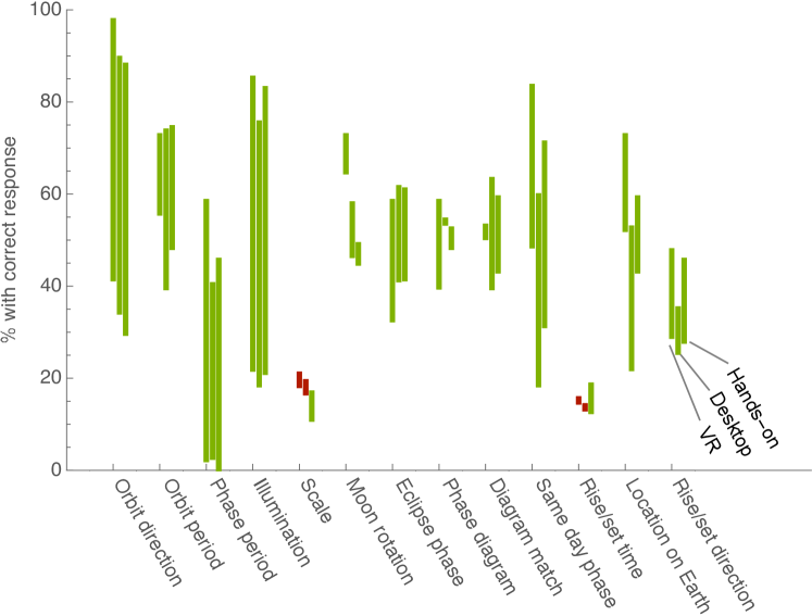
4.3 Attitudes towards the conditions
Consistent with previous work (Dede, 2009) participants overwhelmingly (, ) preferred the VR condition as their favorite learning method independent of their study condition (Fig. 4.5).
78% preferred the VR condition and when describing their reason used phrases such as: the VR condition was “easier to visualize”, “more realistic”, “more immersive”, “more fun”, “more interesting”, and “the most accurate”.
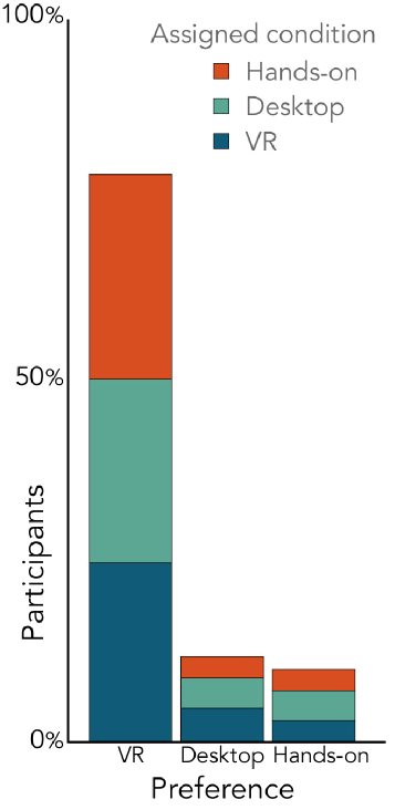
The participants who preferred VR generally said that seeing the full picture in a realistic way helped with their learning. The main contributors to this feeling were the ease of viewing different perspectives and having easier control over the system. For example, one participant wrote:
“Having a overall space to see where everything is helps a lot. Even in class I still had a hard time understanding what they are talking about in concept. But I think I learned a lot in VR and being able to manipulate the environment on my own accord. It seems more engaging than the 2 other methods.”
For the few students who did not prefer VR, participants said that they “did not notice everything that was going on”, found it “a little too complex”, it “made me dizzy and confused,” or generally indicated feeling uncomfortable or overwhelmed. They preferred either the hands-on or desktop conditions because they were more familiar. For example, a participant who preferred the desktop condition wrote:
“The VR was cool but since I’m very new to it I spent most of my time just trying to figure out how it worked–it was also tough to find where the Sun and Moon were at times because of how ‘large’ the environment was. The desktop game was more familiar and easy-to-use for me. Personally.”
The 12% of participants who preferred the desktop condition also used phrases such as: the desktop condition was “less overwhelming”, “easier to control”, and “very easy to follow”. When participants did not like the desktop condition they said: the desktop condition “gave a limited field of view”, and “[was] a lot harder for me to navigate”.
The 10% of participants who preferred the hands-on condition used phrases such as “easiest and fastest”, “I was able to more clearly focus”, and “I got distracted by the other methods”. A participant who preferred the hands-on condition wrote:
“I really liked the virtual reality method. And it gave me more information than the other two methods, for instance, what time of day certain Moon phases would rise and set. Nevertheless, it was almost too overwhelming and it was as if I was too excited to be in space to actually commit to learning the Moon phases. With the hands-on demonstration. there was nothing to distract me. And, obviously, controlling the demonstration felt about as natural as possible.”
4.4 Effects on Environmental Attitudes
Our second hypothesis, that there would be a main effect of condition on environmental attitudes, such that participants in the VR conditions would evince greater environmental support, was also not supported. A one-way ANOVA found no significant differences in environmental attitudes among treatment groups (means standard error were VR = 5.24 0.09, Desktop = 5.25 0.1, Hands-on = 5.35 0.08; F(2, 169) 0.41, p = .66), suggesting that the methods of learning Moon phases did not affect participants’ environmental attitudes. Although we expected that brief exposure in the VR condition to the unique vantage point of the Earth could possibly increase participants’ concerns for environmental issues (by priming the concept of limited resources), the instrument’s typical use as a trait-level instrument may make it unsurprising that we did not observe such an effect.
4.5 Effects due to participant demographics
We conducted exploratory analyses to identify whether other variables were interacting with participants’ experiences in the three conditions. Based on prior literature, we focused on gender, major, video game experience, and quantity of VR experience. We first explored main effects alone and then explored interactions between the variables and condition. When examining the role of the demographic variables on performance, we found a correlation between video game experience and gender (column 1 of Fig. 4.6), but no correlation between any of the other variables. Therefore, video game experience and gender were analyzed in separate regression models.
Main effects between condition and demographic variables
As shown in Table 4.1, students’ pre-score was a significant predictor of their post-scores across conditions and, again, there was no significant differences in post-score between conditions. We interpret the regression coefficients as the simple effect size, (Baguley, 2009). The main effects model also found that there is a significant effect for major, with science majors slightly outperforming non-science majors, even when controlling for pre-score. Neither participants’ gender, video game experience, or VR experience had significant main effects.
Interactions between condition and demographic variables
Experience in VR did not have a significant interaction with condition (Table 4.2). Notably, this indicates that having experience with VR did not improve students’ learning in the VR condition, even though some students claimed that not having experience in VR impeded their learning.
The interactions with gender and video game experience are more complicated. As seen in Table 4.2, there is an interaction between gender and condition in Model 3, with men outperforming in the VR condition. However, Model 4 indicates that there is a main effect with video game experience (seen as marginally significant in Model 2), and a potential interaction between condition and video game experience. From Fig. 4.6, this interaction is likely understood through the pre-test scores. Only in the hands-on condition do we see differences in pre-test scores between participants with and without video game experience. We believe these results can be understood such that men and participants with video game experience learn more from the VR condition, followed by the desktop and then hands-on conditions. Given the correlation between video game experience and gender, it is unclear which variable is responsible for the differences. This correlation between gender and video game experience may be more clearly understood by elaborating on the type and detailed quantity of video game experience in future studies.
| Model 1 | Model 2 | |||||||||
| Term | B | SE | VIF | B | SE | VIF | ||||
| 4.52 | 0.53 | 8.45 | <.001∗∗∗ | 0.0 | 4.42 | 0.54 | 8.26 | <.001∗∗∗ | 0.0 | |
| 0.50 | 0.08 | 6.65 | <.001∗∗∗ | 1.1 | 0.50 | 0.08 | 6.62 | <.001∗∗∗ | 1.1 | |
| -0.05 | 0.41 | -0.13 | 0.898 | 1.4 | 0.00 | 0.40 | 0.00 | 0.998 | 1.4 | |
| 0.23 | 0.41 | 0.56 | 0.578 | 1.4 | 0.32 | 0.41 | 0.78 | 0.44 | 1.4 | |
| 0.52 | 0.43 | 1.20 | 0.233 | 1.0 | ||||||
| 0.63 | 0.35 | 1.79 | 0.075 | 1.1 | ||||||
| 0.70 | 0.37 | 1.89 | 0.060 | 1.3 | 0.70 | 0.37 | 1.91 | 0.058 | 1.3 | |
| -0.17 | 0.51 | -0.33 | 0.741 | 1.4 | -0.19 | 0.50 | -0.39 | 0.699 | 1.4 | |
| 1.14 | 0.36 | 3.21 | 0.002∗∗ | 1.1 | 1.00 | 0.35 | 2.83 | 0.005∗∗ | 1.2 | |
| 0.325 | 0.330 | |||||||||
| 0.296 | 0.302 | |||||||||
| 748.41 | 758.67 | |||||||||
, ,
| Model 3 | Model 4 | |||||||||
| Term | B | SE | VIF | B | SE | VIF | ||||
| 4.76 | 0.61 | 7.74 | <.001∗∗∗ | 0.0 | 4.15 | 0.65 | 6.38 | <.001∗∗∗ | 0.0 | |
| 0.50 | 0.08 | 6.71 | <.001∗∗∗ | 1.1 | 0.48 | 0.08 | 6.28 | <.001∗∗∗ | 1.1 | |
| -0.55 | 0.72 | -0.77 | 0.443 | 4.4 | 0.83 | 0.79 | 1.05 | 0.296 | 5.7 | |
| -0.25 | 0.68 | -0.36 | 0.719 | 4.0 | 0.55 | 0.75 | 0.73 | 0.465 | 5.1 | |
| -0.76 | 0.67 | -1.14 | 0.258 | 2.6 | ||||||
| 1.42 | 0.58 | 2.43 | 0.016∗ | 3.3 | ||||||
| 0.88 | 0.62 | 1.41 | 0.160 | 3.7 | 0.92 | 0.61 | 1.50 | 0.136 | 3.8 | |
| -0.42 | 0.88 | -0.48 | 0.634 | 4.3 | -1.11 | 0.87 | -1.27 | 0.205 | 4.2 | |
| 1.18 | 0.35 | 3.37 | 0.001∗∗ | 1.1 | 1.06 | 0.36 | 2.99 | 0.003∗∗ | 1.2 | |
| 1.77 | 1.12 | 1.59 | 0.115 | 1.8 | ||||||
| 2.56 | 1.00 | 2.57 | 0.011∗ | 2.2 | ||||||
| 0.28 | 0.89 | 0.32 | 0.752 | 4.3 | -0.17 | 0.87 | -0.20 | 0.841 | 4.4 | |
| -0.66 | 0.90 | -0.73 | 0.467 | 3.4 | -0.74 | 0.90 | -0.83 | 0.407 | 3.5 | |
| -0.18 | 1.29 | 0.14 | 0.888 | 2.5 | -0.09 | 1.28 | -0.07 | 0.943 | 2.5 | |
| 0.95 | 1.15 | 0.83 | 0.409 | 3.6 | 1.78 | 1.14 | 1.56 | 0.120 | 3.5 | |
| -1.82 | 0.84 | -2.17 | 0.03∗ | 3.0 | ||||||
| -0.40 | 0.86 | -0.47 | 0.642 | 2.7 | ||||||
| 0.373 | 0.372 | |||||||||
| 0.321 | 0.321 | |||||||||
| 747.89 | 759.59 | |||||||||
, ,
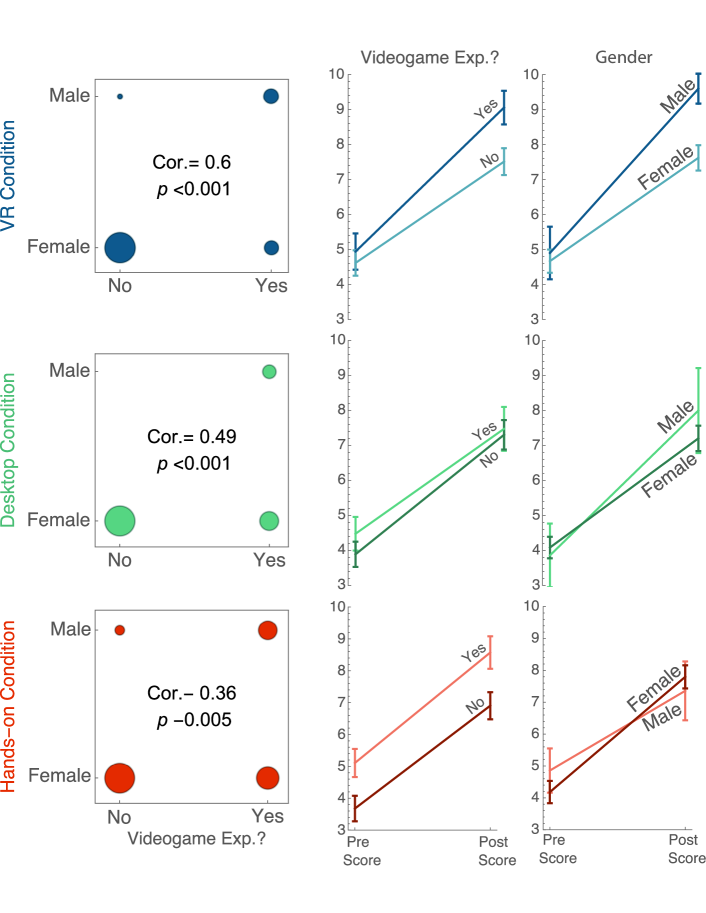
5 Discussion
In this study, we performed a controlled experiment of student learning about
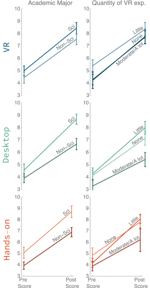
Moon phases through three different modalities: a hands-on activity, a desktop simulation, and a VR simulation.We found no overall effect for condition on students’ learning on an immediate post-test, nor on a delayed post-test four months after the intervention. We did find that students with declared science majors outperformed non-science majors in all conditions. Student learning in the VR condition was not improved with VR experience. Despite these results, students overwhelmingly preferred learning in the VR condition.
There are several possible interpretations of these results. First, our hypothesis had been that the VR simulation would improve performance by reducing the real-world complexities of a hands-on activity and providing a realistic, embodied learning experience. The results suggest that these affordances did not impact learning about Moon phases. On the other hand, one may interpret that the VR condition provided equivalent learning to the other two modalities, while dramatically improving students’ attitudes towards the learning experience.
The study also explored interactions between conditions and students’ video game experience and gender. Gender and video game experience were significantly correlated in our study, and men performed better in the VR condition. This means that either video game experience, being male, or a combination of the two provides an advantage.
There are several studies that suggest video game experience would provide this advantage. One study found that video games can have a beneficial effect on completing complex spatial tasks, visuomotor coordination, and multiple object tracking(Spence and Feng, 2010). Other studies suggest that the benefits of video games on such abilities can be gained after a short time playing an action game and is not dependent on gender (Feng et al., 2007). Furthermore, research has shown that men are more drawn to the type of video games suggested to provide these benefits (Phan et al., 2012). Combining these studies paints a picture that these advantages are not inherently male but may be caused by a particular type of video game experience that so happens to be common for men.
Alternatively, since the 1970’s, several studies have suggested that men have better spatial reasoning than women. However, comprehensive studies have shown recently that, while differences in spatial reasoning between men and women may be present in certain cases, we may not fully understand their causes. Newcombe and Stieff claimed, “from a practical educational standpoint, the most relevant fact is that the relevant skills can be improved in both men and women” (Newcombe and Stieff, 2012, p. 962). Research has also previously found that men outperformed women on post-test conceptual assessments of Moon phase understanding, but only on items involving spatial reasoning (Wilhelm, 2009). However, it has also been found that men’s and women’s scores improve similarly from pre- to post-test with appropriate instruction (Wilhelm, 2009; Jackson et al., 2015), again suggesting that performance can be improved in both men and women.
While our study was unable to prove video game experience was the true contributor to performance increases in the VR condition over gender, literature on the subject suggests that video game experience and not gender may be the affecting variable. While further experimental work should examine this proposition, this points the way to improving learning experiences in virtual reality such that they benefit all learners. If all participants did as well in the virtual reality condition as did men/people with video game experience, then virtual reality could be an overall more effective teaching tool than the other two tested modes of teaching moon phases.
5.1 Limitations
There are several limitations to this study that should be considered when interpreting our results. This study was focused on learning in an activity that was based on physics and astronomy concepts. Thus, we should be careful when applying our findings to learning in other subjects or even other concepts within physics and astronomy (Winn et al., 2002). Furthermore, the participant pool for this study was not perfectly representative of either a typical college classroom or typical physics/astronomy classroom. For example, our study was comprised of 80% women while the American Physical Society reports that only around 20% of undergraduate physics degrees are awarded to women (American Physical Society, 2018). In addition, the significant interaction between gender and condition was based on a small sample of male participants and future work should evaluate this result with more equally distributed samples.
The contribution that we believe this paper makes to the discussion on gender/video game effects on learning in virtual reality is based on exploratory analyses. Thus, future work should explicitly test these hypotheses in a pre-registered study and include more detailed questions related to the type and quantity of video game experience.
While VR technology has advanced rapidly, it is still not ideal. Control responsiveness, motion sickness, limited resolution and field of view are all technological obstacles that can still break immersion and distract from learning using today’s equipment. In contrast, the technologies we used for the hand-on condition and the desktop condition have essentially plateaued compared to VR, meaning the results of this study may change as VR technology progresses.
Compared to VR, the participants were very familiar with the technology used in the hands-on condition and desktop condition. Many participants had never experienced VR before our study or had very limited experience with using a VR headset. This suggests that many of our participants were managing high cognitive load as they attempt to become comfortable with VR, understand the activity, and learn about Moon phases. Participants in the other two conditions did not have such a high barrier to getting comfortable with the technology handed to them. For participants who preferred the non-VR conditions, a common praise was familiarity with the equipment. This suggests that as a college population becomes more familiarly and comfortable using VR, the results of this study may change. Future research should measure students’ cognitive load during the activity explicitly, such as through eye-tracking Zu et al., (2018), self-report surveys Zu et al., (2018); Paas, (1992); Leppink et al., (2013); Paas et al., (2003, 1994), physiological indicators Paas et al., (1994, 2003), or electroencephalography Antonenko et al., (2010). We note, however, that many of the common methods have several limitations de Jong, (2010), such as that different methods may or may not be able to distinguish different types of cognitive load Leppink et al., (2013); DeLeeuw and Mayer, (2008); de Jong, (2010); Paas et al., (2003). It is unclear which may be at play in these activities.
5.2 Future Work
Our study joins others in suggesting that virtual reality is a promising technology as an educational tool but does not, in itself, guarantee a learning advantage over traditional hands-on activities or desktop simulations. There are several areas for future work, based on this analysis.
Future work should focus on further investigating the potential relationship between video game experience and learning gains. This strategy has three components. First, researchers should attempt to sample both male and female participants with equivalent video game experience. Video game experience should be more precisely characterized, focusing on game types that require more visuospatial navigation skills. Video game experiences tend to build procedural or motor skills (Rosser et al., 2007) which do not typically go away after long-term disuse. Measures should thus include lifetime experience, rather than frequency of use alone. If video game experience is confirmed to provide users with skills that allow them to learn better in VR, then researchers can use this knowledge to provide participants with tools to learn to interact with the environment in order to provide a level playing field to all participants.
The VR educational experience can also be improved through enhancing the user interface to maximize VR’s full potential. This does not require waiting for the technology to improve or to become more widely used; instead, designers can take cues from participant’s responses. One strategy would be to enhance users’ sense of embodiment. In this study, users were not embodied in avatars, which may have affected their feeling of presence or ‘being there’ within an environment (Slater, 2017). This in turn could have affected how willing participants were to interact with the environment, thereby reducing their learning gains. Examining existing movement data in the VR condition could provide hints for how to design such a simulation. Similarly, our study used guiding questions that must be answered before proceeding into the environment which may have prevented exploration. Thus, future studies should evaluate how avatar embodiment and interactive text affect movement and learning within an environment as well as how visuospatial ability relates to movement in VR.
Finally, participants worked alone in our study, but each of our conditions could also be used to collaborate. Two students could help each other learn concepts through answering questions together, or an instructor could emphasize key components that are easily missed (Chi, 2009). Indeed in virtual reality in particular, the anonymity can make it a safer space for learning (Yu and Liu, 2009), thereby encouraging students to make mistakes and learn from them without fear of judgement. If participants experience gains from social learning, such gains may be more noticeable in virtual environments.
However, future work must also remain open to the possibility that the excitement and engagement produced by virtual reality experiences may not translate into learning gains in all domains.
6 Conclusion
This study has several takeaway findings. First, participants’ learning gains from pre- to post-test were not significantly different, on average, between the VR, desktop, and hands-on conditions. Participants preformed similarly well on each question topic across the three conditions. We found no strong evidence that participants’ retention differed between conditions after four months. Our hypothesis, that VR would improve learning by simplifying real-world complexities and providing an embodied learning experience, was not supported. Nonetheless, participants strongly favored learning in the VR activity.
Guided by the literature on virtual reality and learning, we also collected data on demographic measures (gender, video game experience, virtual reality experience, and major) to explore predicted interactions, all of which are reported here. We did find a positive effect from gender within the VR condition. However, video game experience and gender were significantly correlated in our study, and the literature suggests that video game experience may be the main reason for the performance increase.
This study has allowed us to determine new experiment designs that will help explore the reasons we saw similar learning gains across conditions. What remains promising about VR is that, relative to a ball on a stick and 2D computer games, it is a technology that is rapidly advancing. Given that participants’ unfamiliarity with VR and the technical roughness of the simulation, the fact that participants were able to learn as much as those in the other conditions may bode well to support VR as a better educational tool when the majority of students are comfortable learning in a virtual environment.
Given that the learning was the same regardless of condition what remains is the fact that participants widely favored the VR experience. As a method of engaging students, using VR was successful in our study and was not achieved at the cost of learning gains. Novelty does diminish however, so an advantage based on novelty alone will cease to be an advantage as exposure rises.
All together, there are many avenues to explore with educational VR. Future work should encourage a more comprehensive look into VR’s ability as an educational tool, such that a participant’s experience is considered from multiple perspectives.
Data Access
DOI for accompanying data: 10.6077/f12c-m973
Acknowledgments
This work was supported by Oculus Education with special thanks to Cindy Ball and Cindi McCurdy. We would like to thank all the graduate and undergraduate students who helped develop the simulations and run participants: Tristan Stone, Yilu Sun, Akhil Gopu, Kristi Lin, Jason Wu, Anirudh Maddula, Frank Rodriguez, Alice Nam, Phil Barrett, Dwyer Tschantz, Connor Lapresi, Giulia Reversi, Keun Youk, Albert Tsao, and Annie Hughey. We would also like to thank Kimberly Williams from the Cornell Center for the Integration of Research, Teaching, and Learning, Stephen Parry of the Cornell Statistical Consulting Unit, Daniel Alexander and Florio Arguillas from the Cornell Institute of Social and Economic Research, and the entire Cornell Physics Education Research Lab for support, comments, and assistance.
7 Supporting information
S1 Table
Modeling interactions between video game experience and gender with condition Supporting data for Fig. 4.6
| Video game experience | |||||||
| Condition | Exp. | Intercept | SE | p | Slope | SE | p |
| VR | Yes | 4.94 | 0.50 | 3.0E-11 | 4.12 | 0.71 | 1.8E-06 |
| VR | No | 4.62 | 0.37 | 7.1E-20 | 2.90 | 0.53 | 5.1E-07 |
| Desktop | Yes | 4.48 | 0.56 | 7.7E-10 | 3.00 | 0.79 | 4.9E-04 |
| Desktop | No | 3.89 | 0.39 | 5.5E-15 | 3.42 | 0.55 | 4.0E-08 |
| Hands-on | Yes | 5.11 | 0.48 | 5.6E-15 | 3.46 | 0.67 | 3.9E-06 |
| Hands-on | No | 3.68 | 0.41 | 1.4E-12 | 3.23 | 0.58 | 7.6E-07 |
| Gender | |||||||
| Condition | Gender | Intercept | SE | p | Slope | SE | p |
| VR | Male | 4.90 | 0.61 | 2.4E-07 | 4.70 | 0.86 | 3.7E-05 |
| VR | Female | 4.67 | 0.35 | 5.2E-23 | 2.96 | 0.49 | 4.1E-08 |
| Desktop | Male | 3.86 | 1.07 | 3.7E-03 | 4.14 | 1.52 | 1.8E-02 |
| Desktop | Female | 4.08 | 0.34 | 4.2E-21 | 3.12 | 0.48 | 2.6E-09 |
| Hands-on | Male | 4.86 | 0.82 | 2.8E-06 | 2.50 | 1.16 | 4.0E-02 |
| Hands-on | Female | 4.18 | 0.36 | 1.6E-19 | 3.61 | 0.50 | 2.5E-10 |
S2 Table
Modeling interactions between academic major, and VR experience quantity with condition Supporting data for Fig. 4.7
| Academic Major | |||||||
| Condition | Major | Intercept | SE | p | Slope | SE | p |
| VR | Science | 5.40 | 0.62 | 1.6E-09 | 3.27 | 0.87 | 8.1E-04 |
| VR | Non-Science | 5.43 | 0.99 | 1.5E-04 | 2.29 | 1.41 | 1.3E-01 |
| Desktop | Science | 4.38 | 0.37 | 1.2E-08 | 3.88 | 0.52 | 3.4E-06 |
| Desktop | Non-Science | 4.17 | 0.79 | 2.7E-05 | 2.17 | 1.12 | 6.5E-02 |
| Hands-on | Science | 5.75 | 0.89 | 1.7E-06 | 2.83 | 1.26 | 3.5E-02 |
| Hands-on | Non-Science | 4.00 | 0.72 | 1.3E-04 | 3.00 | 1.02 | 1.3E-02 |
| Quantity of VR experience | |||||||
| Condition | Quantity | Intercept | SE | p | Slope | SE | p |
| VR | None | 5.41 | 0.52 | 2.8E-13 | 2.95 | 0.73 | 2.2E-04 |
| VR | Little | 4.29 | 0.47 | 2.4E-11 | 3.43 | 0.66 | 6.8E-06 |
| VR | Moderate/A lot | 4.23 | 0.63 | 6.3E-07 | 3.54 | 0.89 | 5.8E-04 |
| Desktop | None | 4.14 | 0.49 | 2.1E-10 | 3.00 | 0.70 | 1.0E-04 |
| Desktop | Little | 4.28 | 0.48 | 3.5E-12 | 3.72 | 0.69 | 1.3E-06 |
| Desktop | Moderate/A lot | 3.29 | 0.55 | 6.2E-05 | 2.14 | 0.77 | 1.7E-02 |
| Hands-on | None | 4.85 | 0.65 | 5.2E-09 | 2.95 | 0.91 | 2.6E-03 |
| Hands-on | Little | 4.17 | 0.41 | 1.7E-14 | 3.90 | 0.58 | 8.3E-09 |
| Hands-on | Moderate/A lot | 3.89 | 0.79 | 1.6E-04 | 2.33 | 1.12 | 5.4E-02 |
![[Uncaptioned image]](/html/2010.05046/assets/art/MFA_d6.jpg)
Chapter 5 High-resolution Spectra for a Wide Range of Habitable Zone Planets around Sun-like stars
This thesis chapter originally appeared in the literature as
J. Madden and L. Kaltenegger, The Astrophysical Journal Letters (2020)
Abstract
The search for life in the universe is currently focused on Earth-analog planets. However, we should be prepared to find a diversity of terrestrial exoplanets not only in terms of host star but also in terms of surface environment. Simulated high-resolution spectra of habitable planets covering a wide parameter space are essential in training retrieval tools, optimizing observing strategies, and interpreting upcoming observations. Ground-based extremely large telescopes like ELT, GMT, and TMT; and future space-based mission concepts like Origins, HabEx, and LUVOIR are designed to have the capability of characterizing a variety of potentially habitable worlds. Some of these telescopes will use high precision radial velocity techniques to obtain the required high-resolution spectra () needed to characterize potentially habitable exoplanets.
Here we present a database of high-resolution (0.01 cm-1) reflection and emission spectra for simulated exoplanets with a wide range of surfaces, receiving similar irradiation as Earth around 12 different host stars from F0 to K7.
Depending on surface type and host star, we show differences in spectral feature strength as well as overall reflectance, emission, and star to planet contrast ratio of terrestrial planets in the Habitable zone of their host stars. Accounting for the wavelength-dependent interaction of the stellar flux and the surface will help identify the best targets for upcoming spectral observations in the visible and infrared.
All of our spectra and model profiles are available online.
1 Introduction
Currently, about 4000 extrasolar planets have been detected orbiting Main Sequence stars with dozens of terrestrial planets orbiting in their habitable zone (HZ) (Kane et al., 2016; Johns et al., 2018; Berger et al., 2018). The detected rocky exoplanets in the HZ show a wide variety of sizes and stellar hosts. For now, we are unable to characterize their atmospheres.
If our Solar System is any indication (e.g. Madden and Kaltenegger, 2018; Krissansen-Totton et al., 2016; Cahoy et al., 2010; Lundock et al., 2009; Traub, 2003), exoplanets should show a large diversity in composition and surface type. Therefore, it is important to model a wide range of surfaces and stellar hosts for rocky planets to expand the spectral database we will use to characterize planets and search for signs of life in their atmospheres.
Direct observations that provide reflection and emission spectra of habitable zone exoplanets are critical to identifying signs of life on exoplanets (e.g. Kaltenegger, 2017; Schwieterman et al., 2018; Fujii et al., 2018) and should be within the capabilities of the next generation of ground-based telescopes like the extremely large telescopes (ELTs) and mission concepts such as Origins, HabEx, and LUVOIR (e.g. Arney et al., 2018; Snellen et al., 2017). Spectrographs on the Extremely Large Telescope (ELT) like HIRES (0.3-2.5) and METIS (3-19) are designed for a resolution of (Ramsay et al., 2020). Our database provides spectra modelled at 0.01, which translates into a minimum resolution of from 0.4 to 10 and a minimum of from 10 to 20
Here we present a high-resolution database of 360 reflection and emission spectra of Earth-like planets with diverse surfaces, which evolved in the HZ of a wide range of Sun-like host stars. Our spectra are based on the atmosphere models described in detail in Madden and Kaltenegger, 2020b .
This database enables us to explore which of these planets provide the strongest atmospheric features for overall characterization as well as signs of life. Biosignatures in this work represent disequilibrium atmospheric chemistry suggesting biotic sources, namely the biosignature pairs of O2 and CH4, and CH4 and O3 (Lovelock, 1965b ; Lederberg, 1965).
Our high-resolution spectra show the effects surfaces and host stars can have on the detectability of atmospheric features of habitable-zone planets and is a tool to prioritize promising targets in upcoming observations.
Our spectra provide an important step in expanding the references used for optimizing upcoming observations, training retrieval algorithms as well as providing comparison model datasets to analyze future observations. In addition, studies show that high-resolution () exoplanet spectrum can be isolated from the combined star-planet spectrum, using the radial velocity difference between the two objects (Snellen et al., 2015; Rodler and López-Morales, 2014; Brogi et al., 2014; Fischer et al., 2016; Lopez-Morales et al., 2019). high-resolution spectra models of habitable atmospheres are important in refining this technique and may allow characterization of planets even if they can’t be resolved.
Section 2 describes our models, section 3 presents our results, and section 4 discusses and summarizes our paper.
Our high-resolution spectra are available online at DOI: 10.5281/zenodo.3912065.
2 Methods
2.1 Planetary and Atmospheric Model
The atmospheric composition of Earth-like planets depends on the outgassing rates, the irradiation from its host star, subsequent photochemistry, surface type, and cloud coverage. Here, we define ‘Earth-like’ to refer to an Earth-radius and Earth-mass planet with similar outgassing rates to the modern Earth. Our spectra use planetary models generated using a coupled 1D climate and photochemistry model with wavelength-dependent albedo, described in detail in Madden and Kaltenegger, 2020b .
By incorporating wavelength-dependent reflection of surfaces and decoupling clouds from the surface reflection Madden and Kaltenegger, 2020b explored the relationship between surface type and stellar type in the context of habitability. Madden and Kaltenegger, 2020b found that surfaces with high variability across the visible and near-IR displayed a wide range of surface temperatures across star type. Surfaces like vegetation and sand showed the biggest change in surface temperature between cool K and hot F-stars while flatter overall albedo such as basalt, granite, coast, and seawater showed less change in surface temperature between star type. The surface temperature ranges for the different planet models are shown in Table 5.1.
2.2 Generating reflection and emission spectra
We use EXO-Prime2 to generate the high-resolution reflection and emission spectra for each simulated exoplanet from 0.4 to 20 at a resolution of . The radiative transfer model used was originally developed for stratospheric measurements in Earth’s atmosphere (Traub and Stier, 1976; Traub and Jucks, 2002) and has been updated for use with exoplanets (e.g. Des Marais et al., 2002; Traub and Jucks, 2002; Kaltenegger et al., 2007; Kaltenegger and Traub, 2009; O’Malley-James and Kaltenegger, 2019). For our calculations, we used 38 plane-parallel layers for an 80km atmosphere with an observation zenith angle of 60 degrees giving an approximation of quadrature viewing.
| Surface | Source | Temp. Range | Temp. |
|---|---|---|---|
| (K) | (K) | ||
| (F0V-K7V) | |||
| Basalt | ASTER Basalt: Solid: Basalt.H5 | 315.5-296.4 | 19.1 |
| Granite | ASTER Alkalic: Solid: Granite.H1 | 314.4-295.2 | 19.2 |
| Sand | ASTER Brown loamy fine: 87P3468 | 311.8-280.2 | 31.6 |
| Grass | ASTER Grass: Unknown | 314.7-280.8 | 33.9 |
| Trees | ASTER Deciduous: Unknown | 312.4-278.8 | 33.6 |
| Seawater | USGS Open Ocean SW2 (0.2-2.4) | 326.4-304.7 | 21.7 |
| ASTER Seawater: Liquid (2.4+) | |||
| Coast | USGS Coast SW1 (0.2-2.4) | 326.6-303.9 | 22.7 |
| ASTER Seawater: Liquid (2.4+) | |||
| Cloud | Modis Cloud Model | 249.9-260.0 | -10.1 |
| Basalt+Cloud | 56.3% Basalt, 43.7% Cloud | 286.7-281.9 | 4.8 |
| Granite+Cloud | 56.3% Granite, 43.7% Cloud | 286.1-280.8 | 5.3 |
| Sand+Cloud | 56.3% Sand, 43.7% Cloud | 284.0-271.9 | 12.1 |
| Grass+Cloud | 56.3% Grass, 43.7% Cloud | 285.0-272.7 | 13.8 |
| Trees+Cloud | 56.3% Trees, 43.7% Cloud | 283.9-270.1 | 12.3 |
| Seawater+Cloud | 56.3% Seawater, 43.7% Cloud | 297.0-287.8 | 9.2 |
| Coast+Cloud | 56.3% Coast, 43.7% Cloud | 297.1-287.9 | 9.2 |
| Basalt+Seawater | 30% Basalt, 70% Seawater | 323.1-302.7 | 20.4 |
| Granite+Seawater | 30% Granite, 70% Seawater | 322.9-302.1 | 20.8 |
| Sand+Seawater | 30% Sand, 70% Seawater | 322.5-299.2 | 23.3 |
| Grass+Seawater | 30% Grass, 70% Seawater | 323.2-299.0 | 24.1 |
| Trees+Seawater | 30% Trees, 70% Seawater | 322.7-298.6 | 24.2 |
| Snow+Seawater | 30% Snow, 70% Seawater | 290.6-288.5 | 2.1 |
| Basalt+Seawater+Cloud | 56.3% (Basalt+Seawater), 43.7% Cloud | 293.7-286.1 | 7.6 |
| Granite+Seawater+Cloud | 56.3% (Granite+Seawater), 43.7% Cloud | 293.5-285.9 | 7.6 |
| Sand+Seawater+Cloud | 56.3% (Sand+Seawater), 43.7% Cloud | 292.6-283.1 | 9.5 |
| Grass+Seawater+Cloud | 56.3% (Grass+Seawater), 43.7% Cloud | 293.1-283.4 | 9.5 |
| Trees+Seawater+Cloud | 56.3% (Trees+Seawater), 43.7% Cloud | 292.6-283.1 | 9.7 |
| Snow+Seawater+Cloud | 56.3% (Snow+Seawater), 43.7% Cloud | 277.9-277.2 | 0.7 |
| Earth | 70% Seawater, 2% Coast, 2.52% Basalt, | 319.6-298.6 | 21.0 |
| 2.52% Granite, 1.96% Sand, 8.4% Grass, | |||
| 8.4% Trees, 4.2% Snow | |||
| Earth+Cloud | 56.3% Earth, 43.7% Cloud | 290.4-283.1 | 7.3 |
| Flat | Flat reflectence of 0.31 | 291.3-280.8 | 10.5 |
We include the molecular species with prominent absorption features expected in the atmospheres of Earth-like planets orbiting F to K stars as modeled in Madden and Kaltenegger, 2020b . We use the 2016 HITRAN database for our opacities for H2O, CO2, CH4, N2O, O3, O2, H2CO, OH, C2H6, HO2, CO, NO, NO2, H2O2, H2S, and SO2 (Gordon et al., 2017). We include CO2 line mixing (Niro et al., 2005). For CO2, H2O, and N2, we use measured continua data instead of line-by-line calculations in the far wings (Traub and Jucks, 2002).
With no clear answer on how cloud-feedback should affect clouds on exoplanets orbiting different host stars, we use Earth’s clouds as a first approximation for all our models. We include 3 cloud layers in our models (following Kaltenegger et al., (2007)) at 1km (40%), 6km (40%), and 12km (20%) and an overall cloud coverage of 44% (Madden and Kaltenegger, 2020b ). This simulates an observation of a cloudy exoplanet by having the spectrum represent the sum of different layers in the atmosphere.
2.3 Stellar Spectra & Surface Albedos
The effects of wavelength-dependent surface and cloud albedo on habitability are most apparent when comparing the planetary models across star type. We used the same ATLAS model (Castelli and Kurucz, 2004) F, G, and K star as in Madden and Kaltenegger, 2020b for our calculations of planetary spectra and star to planet contrast. In total, we simulated planets around 12 star types spaced roughly 250K in temperature between an F0V (7,400K) and a K7V (3,900K). Note that the simulations in Madden and Kaltenegger, 2020b used lower total stellar incident flux on the planet for cooler host stars to achieve temperatures similar to modern Earth across star type ( percent).
The albedos used here and in Madden and Kaltenegger, 2020b focus on the dominant surfaces on Earth: seawater, coastal water, basalt, granite, sand, trees, grass, snow, and clouds. A modern Earth albedo can be made by combining these surfaces with weights based on their modern Earth surface coverage (Kaltenegger et al., 2007). Surface albedos were taken from the USGS and ASTER spectral libraries (Baldridge et al., 2009; Kokaly et al., 2017; Clark et al., 2007). For all three cloud layers, we use the Modis cloud albedo (King et al., 1997; Rossow and Schiffer, 1999) (Table 5.1).
In this paper we show four planetary scenarios for each surface: i) a single planetary surface to show the maximum effect of a specific surface on the spectra, ii) a 30% single surface and 70% seawater combination, and iii) and iv) two more scenarios where these cases have the 44% cloud coverage, derived to simulate the modern Earth model in Madden and Kaltenegger, 2020b .
For 30 different surfaces around 12 host star types, we simulated in total, 360 terrestrial planetary spectra from 0.4 to 20.
3 Results
Our high-resolution spectra database contains the combined reflection and emission spectra for 360 Earth-like planets with 30 different surfaces orbiting 12 different Sun-like host stars. All spectra shown are a combination of planet reflection and emission. Emission begins to dominate the flux between 3 and 4 depending on the star and surface temperature.
We highlight a subset of these spectra in our figures to show a balance of variety and specific effects while keeping figures uncrowded. We do not show the simulated spectra for granite, grass, coast, or cloud surface only. The surface reflectivity of granite is similar to first-order with basalt, grass with trees, and coast with seawater. However, these spectra can all be downloaded from our database.
3.1 Reflection Spectra
The star-surface interaction leads to drastic differences in a planet’s appearance, which are most apparent in the exoplanets’ reflectance spectra in the visible.
Even though the incident stellar flux decreases for cooler star types to provide similar surface temperatures in our models, the reflected flux of a planet can vary by more than an order of magnitude at specific wavelengths depending on a planet’s surface reflectivity, as shown in Fig. 5.1, and Fig. 5.2. It can result in planets with highly reflective surfaces orbiting cooler stars reflecting more starlight than planets with low surface reflectivity orbiting hotter stars: For example, at , a desert planet (sand surface) orbiting a K7V star is twice as bright as an ocean planet (seawater surface) orbiting an F0V host star, despite the higher incident flux of an F0V star at that wavelength.
Surfaces with high reflectivity generally lead to more prominent spectral features at visible wavelengths. The deepest absorption features can be seen for planetary models with high reflective surfaces like vegetation, sand, and snow orbiting the hottest grid host stars, which provide the highest incident flux (Fig. 5.1 and 5.2).
The shape of the surface albedo also modulates the flux of the visible exoplanet spectra models. For example, the vegetation ’red-edge’ near shows as a strong increase in reflectivity in the spectra of tree-covered planets (Fig. 5.1 and Fig. 5.2).
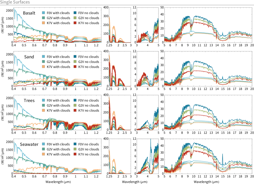
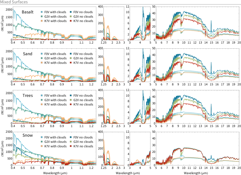
3.2 Emission
Planetary surface albedos can have a large effect on the planetary surface temperature as well as atmospheric temperature structure (Madden and Kaltenegger, 2020b ). Planetary models with highly reflective surfaces generally lead to lower surface temperatures and therefore lower infrared emission, while models with less reflective surfaces lead to higher surface temperatures and thus higher infrared emission of the planet for a specific host star (Table 5.1, Fig. 5.1 and 5.2).
The models in Madden and Kaltenegger, 2020b used a reduced incident flux for cooler stars to achieve similar modern Earth temperatures for a constant surface albedo of 0.31. Therefore, while the surface reflectivity of a planet changes the surface temperature for similar incident flux, that difference has been compensated for in the modeling for a specific wavelength-independent surface albedo case, resulting in a slight increase in surface temperature and overall emission for planets orbiting hotter host stars (see Fig. 5.1 and 5.2).
Infrared spectral feature depth depends on both the abundance as well as the difference in temperature of the overall emitting and absorption layer. Thus the deepest absorption features are not seen for the hottest planetary models with low reflective surfaces like oceans (Fig. 5.1 and 5.2), because of the similarity in temperature of the two layers compared to planets with different surfaces.
3.3 Planet-to-star contrast
Planet-star contrast is generally higher for similar planets around cooler stars versus hotter stars. Fig. 5.3 shows that Earth-like planets orbiting our coolest grid stars have the highest contrast across the spectrum compared to hotter host stars. Planets with the same surface also show this based on our spectra (Fig. 5.4).
However, an ocean planet covered with dark seawater orbiting a K7V-star shows a similar contrast ratio in the visible and near-infrared () as a planet covered in vegetation around an F0V host star (Fig. 5.4). Planets covered by highly reflective surfaces such as grass, trees, snow, and sand around G-stars will be consistently as high or higher in contrast at visible wavelengths than planets covered by darker surfaces such as coast, seawater, basalt, or granite around K-stars. Therefore, a planet’s surface can influence the contrast ratio significantly in the visible and near-IR. When comparing surfaces with extreme differences in reflectivity, cooler stars may not always provide the highest contrast habitable zone targets in the visible and near-IR, depending on their surface composition.

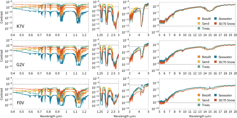
3.4 Atmospheric composition change with host star
The stellar energy distribution (SED) of a star influences the atmospheric composition of a planet (Kasting et al., 1993; Rugheimer et al., 2013; Rugheimer et al., 2015a ; Segura et al., 2003, 2005; Madden and Kaltenegger, 2020b ; Rauer et al., 2011). Fig. 5.3, Fig. 5.1, and Fig. 5.2 show the varying depth of the atmospheric spectral features such as O3, CO2, and CH4 for different stellar hosts.
In the visible, the depth of an absorption feature is proportional to the abundance of a molecule, the amount of incident stellar radiation, and the reflectivity of the planet. For similar reflectivity, the change in the absorption features depth reflects the change in abundance of the chemicals due to the stellar SED and subsequent photochemistry in the planet’s atmosphere as well as incident irradiation (Fig. 5.3). Hotter stars in our grid emit higher UV flux, thus altering the profiles of these molecules and subsequent reactions in a planet’s atmosphere
In the infrared, the depth of the absorption features depends on the abundance of a chemical as well as the temperature difference between the emitting/absorbing layer and the continuum.
Surfaces can modify the atmosphere composition based on how the surface albedo alters the surface temperature of the planet as well as the temperature profiles of the atmosphere, for example how much water is evaporated.
Fig. 5.3 shows the change in planet-to-star contrast ratio for a planet model with a modern Earth-analog surface for our grid stars to isolate the effect of the host star on the planet’s spectra.
The most notable spectral features between 0.4 and 20 relevant to biosignature detection include oxygen and ozone at 0.69, 0.76, and 9.6; in combination with methane at 0.88, 1.04, 2.3, 3.3, and 7.66; ; N2O shows features at 7.75, 8.52, 10.65, and 16.89. H2O has features at 0.6, 0.65. 0.73, 0.82, 0.95, 1.14, 1.4, 1.85, 2.5-3.5, 3.7, and 5-8. Another greenhouse gas seen in the spectra is CO2 at 2.7, 4.25, and 15.
As an example, for the 0.76 O2 and the 9.6 O3 feature, Fig. 5.5 shows that at a high-resolution of , all spectral features have a distinct series of lines to identify such Doppler-shifted lines uniquely on exoplanets which move predictably around their host star (Rodler and López-Morales, 2014; Snellen et al., 2015; Brogi et al., 2014). For specific absorption features of interest, our high-resolution spectra database can be used to optimize observation strategies for specific features and specific wavelength regions.
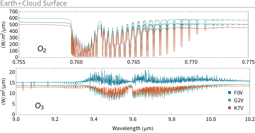
4 Discussion & Conclusion
We present 360 emission and reflection spectra at a high-resolution of for habitable zone planets orbiting 12 F, G, and K star types. These model spectra show the interaction of the host star’s stellar energy distribution and a planet’s wavelength-dependent albedo. We used the 9 dominant surfaces on modern Earth and isolated the effects of rock (basalt and granite), vegetation, sand, snow, clouds, water (ocean and coast) as well as clouds on a planet’s reflection and emission spectra from the visible to the infrared (0.4-20).
To show the variety in this database, we include models with single surface planets to show the maximum effect of each surface on the spectra as well as the planet star to planet contrast ratio (Fig. 5.4 and 5.1), mixtures of seawater and cloud coverage (Fig. 5.1 and 5.2) as well as modern Earth surface coverage models (Fig. 5.3) for the 12 host stars from F0V to K7V.
Other surface albedos and fractional combinations of surfaces are of course possible for exoplanets. As a first-order estimate our single surface spectra can be combined to create spectra for new surface mixtures. In this way, our spectral database provides a toolkit to generate estimated spectra of Earth-like planets with different surface combinations with and without clouds. One aspect that won’t be captured by such a combination is the potential difference in surface temperature introduced by the different surface reflectivity (see Madden and Kaltenegger, 2020b ). Exoplanets may also have many different surface types not addressed in this study including mineral surfaces(Shields and Carns, 2018), a wide range of different biota (Hegde and Kaltenegger, 2013) or biofluorescent organisms(O’Malley-James and Kaltenegger, 2018a ).
We’ve shown that surface albedos can deepen spectral features. In the visible, where the spectra show reflected starlight, highly reflective surfaces generally increase the depth of absorption features. In the infrared, on the other hand, low reflective surfaces increase the surface temperature and thus a planet’s overall emission.
Our high-resolution spectra database provides a critical tool in the planning and analysis of observations with upcoming ground-based telescopes like ELT, GMT, and TMT and future space mission concepts Origins, HabEx, and LUVOIR. Ground-based telescopes plan to employ high precision radial velocity techniques that require high-resolution () in order to characterize potentially habitable exoplanets.
Studying the wide range of changes caused by different surfaces and host stars improves our understanding of biosignatures and their remote observability. Obtaining high-resolution spectra of terrestrial planets in the habitable zone is an essential milestone in discovering life beyond our Solar System. Our database is intended to support this objective by presenting a wide range of cases for further study, planning, training, and comparison.
Data Access
DOI for accompanying data: 10.5281/zenodo.3912065
Acknowledgments
This work was supported by the Carl Sagan Institute and the Brinson Foundation.
![[Uncaptioned image]](/html/2010.05046/assets/art/MFA_d8.jpg)
References
- Abbot et al., (2018) Abbot, D. S., Bloch-Johnson, J., Checlair, J., Farahat, N. X., Graham, R. J., Plotkin, D., Popovic, P., and Spaulding-Astudillo, F. (2018). Decrease in Hysteresis of Planetary Climate for Planets with Long Solar Days. ApJ, 854(1):3.
- Abe et al., (2011) Abe, Y., Abe-Ouchi, A., Sleep, N. H., and Zahnle, K. J. (2011). Habitable Zone Limits for Dry Planets. Astrobiology, 11(5):443–460.
- Ahn et al., (2016) Ahn, S. J., Bostick, J., Ogle, E., Nowak, K. L., McGillicuddy, K. T., and Bailenson, J. N. (2016). Experiencing nature: Embodying animals in immersive virtual environments increases inclusion of nature in self and involvement with nature. Journal of Computer-Mediated Communication, 21(6):399–419.
- Airapetian et al., (2017) Airapetian, V. S., Glocer, A., Khazanov, G. V., Loyd, R. O. P., France, K., Sojka, J., Danchi, W. C., and Liemohn, M. W. (2017). How Hospitable Are Space Weather Affected Habitable Zones? The Role of Ion Escape. ApJ, 836(1):L3.
- American Physical Society, (2018) American Physical Society (2018). Bachelor’s degrees in physics and stem earned by women. https://www.aps.org/programs/education/statistics/womenstem.cfm.
- Anderson, (2003) Anderson, M. L. (2003). Embodied cognition: A field guide. Artificial Intelligence, 149(1):91 – 130.
- Antonenko et al., (2010) Antonenko, P., Paas, F., Grabner, R., and van Gog, T. (2010). Using Electroencephalography to Measure Cognitive Load. Educational Psychology Review, 22(4):425–438.
- Arney et al., (2018) Arney, G., Batalha, N., Cowan, N., Domagal-Goldman, S., Dressing, C., Fujii, Y., Kopparapu, R., Lincowski, A., Lopez, E., Lustig-Yaeger, J., and Youngblood, A. (2018). The Importance of Multiple Observation Methods to Characterize Potentially Habitable Exoplanets: Ground- and Space-Based Synergies. arXiv e-prints, page arXiv:1803.02926.
- Arney et al., (2016) Arney, G., Domagal-Goldman, S. D., Meadows, V. S., Wolf, E. T., Schwieterman, E., Charnay, B., Claire, M., Hébrard, E., and Trainer, M. G. (2016). The Pale Orange Dot: The Spectrum and Habitability of Hazy Archean Earth. Astrobiology, 16(11):873–899.
- Aymerich-Franch et al., (2012) Aymerich-Franch, L., Karutz, C., and Bailenson, J. N. (2012). Effects of facial and voice similarity on presence in a public speaking virtual environment. In Proceedings of the International Society for Presence Research Annual Conference, pages 24–26.
- Baguley, (2009) Baguley, T. (2009). Standardized or simple effect size: What should be reported? British Journal of Psychology, 100(3):603–617.
- Baldridge et al., (2009) Baldridge, A. M., Hook, S., Grove, C., and Rivera, G. (2009). The aster spectral library version 2.0. Remote Sensing of Environment, 113(4):711–715.
- Barstow and Irwin, (2016) Barstow, J. K. and Irwin, P. G. J. (2016). Habitable worlds with JWST: transit spectroscopy of the TRAPPIST-1 system? Monthly Notices of the Royal Astronomical Society, 461(1):L92–L96.
- Battersby et al., (2018) Battersby, C., Armus, L., Bergin, E., Kataria, T., Meixner, M., Pope, A., Stevenson, K. B., Cooray, A., Leisawitz, D., Scott, D., Bauer, J., Bradford, C. M., Ennico, K., Fortney, J. J., Kaltenegger, L., Melnick, G. J., Milam, S. N., Narayanan, D., Padgett, D., Pontoppidan, K., Roellig, T., Sandstrom, K., Su, K. Y. L., Vieira, J., Wright, E., Zmuidzinas, J., Staguhn, J., Sheth, K., Benford, D., Mamajek, E. E., Neff, S. G., Carey, S., Burgarella, D., De Beck, E., Gerin, M., Helmich, F. P., Moseley, S. H., Sakon, I., and Wiedner, M. C. (2018). The Origins Space Telescope. Nature Astronomy, 2:596–599.
- Belton et al., (1981) Belton, M. J. S., Wallace, L., and Howard, S. (1981). The periods of Neptune - Evidence for atmospheric motions. Icarus, 46:263–274.
- Berger et al., (2018) Berger, T. A., Huber, D., Gaidos, E., and van Saders, J. L. (2018). Revised Radii of Kepler Stars and Planets Using Gaia Data Release 2. ApJ, 866(2):99.
- Bessell, (1979) Bessell, M. S. (1979). UBVRI photometry. II - The Cousins VRI system, its temperature and absolute flux calibration, and relevance for two-dimensional photometry. PASP, 91:589–607.
- Bétrémieux and Kaltenegger, (2014) Bétrémieux, Y. and Kaltenegger, L. (2014). Impact of Atmospheric Refraction: How Deeply can We Probe Exo-Earth’s Atmospheres during Primary Eclipse Observations? ApJ, 791(1):7.
- Bin et al., (2018) Bin, J., Tian, F., and Liu, L. (2018). New inner boundaries of the habitable zones around M dwarfs. Earth and Planetary Science Letters, 492:121–129.
- Boschi et al., (2013) Boschi, R., Lucarini, V., and Pascale, S. (2013). Bistability of the climate around the habitable zone: A thermodynamic investigation. Icarus, 226(2):1724–1742.
- Bransford et al., (1999) Bransford, J., Brown, A., and Cocking, R. (1999). How people learn: Mind, brain, experience, and school. Washington, DC: National Research Council.
- Bricken, (1991) Bricken, M. (1991). Virtual reality learning environments: Potentials and challenges. SIGGRAPH Comput. Graph., 25(3):178–184.
- Brierley et al., (2009) Brierley, C. M., Fedorov, A. V., Liu, Z., Herbert, T. D., Lawrence, K. T., and LaRiviere, J. P. (2009). Greatly expanded tropical warm pool and weakened hadley circulation in the early pliocene. Science, 323(5922):1714–1718.
- Brogi et al., (2014) Brogi, M., de Kok, R. J., Birkby, J. L., Schwarz, H., and Snellen, I. A. G. (2014). Carbon monoxide and water vapor in the atmosphere of the non-transiting exoplanet HD 179949 b. A&A, 565:A124.
- Brown et al., (1989) Brown, J. S., Collins, A., and Duguid, P. (1989). Situated Cognition and the Culture of Learning. Educational Researcher, 18(1):32.
- Buratti and Veverka, (1983) Buratti, B. and Veverka, J. (1983). Voyager photometry of Europa. Icarus, 55:93–110.
- Cahoy et al., (2010) Cahoy, K. L., Marley, M. S., and Fortney, J. J. (2010). Exoplanet Albedo Spectra and Colors as a Function of Planet Phase, Separation, and Metallicity. ApJ, 724:189–214.
- Carbonneau et al., (2013) Carbonneau, K. J., Marley, S. C., and Selig, J. P. (2013). A meta-analysis of the efficacy of teaching mathematics with concrete manipulatives. Journal of Educational Psychology, 105(2):380–400.
- Castelli and Kurucz, (2004) Castelli, F. and Kurucz, R. L. (2004). New grids of atlas9 model atmospheres. ArXiv Astrophysics e-prints.
- Chang et al., (2016) Chang, H.-Y., Hsu, Y.-S., and Wu, H.-K. (2016). A comparison study of augmented reality versus interactive simulation technology to support student learning of a socio-scientific issue. Interactive Learning Environments, 24(6):1148–1161.
- Chen et al., (2019) Chen, H., Wolf, E. T., Zhan, Z., and Horton, D. E. (2019). Habitability and Spectroscopic Observability of Warm M-dwarf Exoplanets Evaluated with a 3D Chemistry-Climate Model. ApJ, 886(1):16.
- Chi, (2009) Chi, M. T. H. (2009). Active-Constructive-Interactive: A Conceptual Framework for Differentiating Learning Activities. Topics in Cognitive Science, 1(1):73–105.
- Chini et al., (2012) Chini, J. J., Madsen, A., Gire, E., Rebello, N. S., and Puntambekar, S. (2012). Exploration of factors that affect the comparative effectiveness of physical and virtual manipulatives in an undergraduate laboratory. Physical Review Special Topics - Physics Education Research, 8(1):010113.
- Clark et al., (2007) Clark, R. N., Swayze, G. A., Wise, R. A., Livo, K. E., Hoefen, T. M., Kokaly, R. F., and Sutley, S. J. (2007). Usgs digital spectral library splib06a. Technical report, US Geological Survey.
- Cockell et al., (2009) Cockell, C. S., Kaltenegger, L., and Raven, J. A. (2009). Cryptic Photosynthesis-Extrasolar Planetary Oxygen Without a Surface Biological Signature. Astrobiology, 9(7):623–636.
- Cole et al., (2018) Cole, M., Cohen, C., Wilhelm, J., and Lindell, R. (2018). Spatial thinking in astronomy education research. Physical Review Physics Education Research, 14(1):010139.
- Cortina, (1993) Cortina, J. M. (1993). What is coefficient alpha? an examination of theory and applications. Journal of Applied Psychology, 78:98–104.
- Council, (2010) Council, N. R. (2010). New Worlds, New Horizons in Astronomy and Astrophysics. The National Academies Press, Washington, DC.
- Cousins, (1976) Cousins, A. (1976). Standard Stars for VRI Photometry with S25 Response Photocathodes. Monthly Notes of the Astronomical Society of South Africa, 35:70.
- Crouch et al., (2004) Crouch, C., Fagen, A. P., Callan, J. P., and Mazur, E. (2004). Classroom demonstrations: Learning tools or entertainment? American Journal of Physics, 72(6):835–838.
- Cunningham, (1946) Cunningham, H. A. (1946). Lecture demonstration versus individual laboratory method in science teaching—A summary. Science Education, 30(2):70–82.
- Darrah et al., (2014) Darrah, M., Humbert, R., Finstein, J., Simon, M., and Hopkins, J. (2014). Are Virtual Labs as Effective as Hands-on Labs for Undergraduate Physics? A Comparative Study at Two Major Universities. Journal of Science Education and Technology, 23(6):803–814.
- de Jong, (2010) de Jong, T. (2010). Cognitive load theory, educational research, and instructional design: some food for thought. Instructional Science, 38(2):105–134.
- de Vaucouleurs, (1964) de Vaucouleurs, G. (1964). Geometric and Photometric Parameters of the Terrestrial Planets. Icarus, 3:187–235.
- Dede, (2009) Dede, C. (2009). Immersive interfaces for engagement and learning. science, 323(5910):66–69.
- DeLeeuw and Mayer, (2008) DeLeeuw, K. E. and Mayer, R. E. (2008). A comparison of three measures of cognitive load: Evidence for separable measures of intrinsic, extraneous, and germane load. Journal of Educational Psychology, 100(1):223–234.
- Des Marais et al., (2002) Des Marais, D. J., Harwit, M. O., Jucks, K. W., Kasting, J. F., Lin, D. N. C., Lunine, J. I., Schneider, J., Seager, S., Traub, W. A., and Woolf, N. J. (2002). Remote Sensing of Planetary Properties and Biosignatures on Extrasolar Terrestrial Planets. Astrobiology, 2:153–181.
- Dunlap and Liere, (2008) Dunlap, R. E. and Liere, K. D. V. (2008). The ”new environmental paradigm”. The Journal of Environmental Education, 40(1):19–28.
- Dunlap and Van Liere, (1978) Dunlap, R. E. and Van Liere, K. D. (1978). The “new environmental paradigm”. The journal of environmental education, 9(4):10–19.
- Dunlap et al., (2000) Dunlap, R. E., Van Liere, K. D., Mertig, A. G., and Jones, R. E. (2000). New trends in measuring environmental attitudes: Measuring endorsement of the new ecological paradigm: A revised nep scale. Journal of Social Issues, 56(3):425–442.
- Dyudina et al., (2016) Dyudina, U., Zhang, X., Li, L., Kopparla, P., Ingersoll, A. P., Dones, L., Verbiscer, A., and Yung, Y. L. (2016). Reflected light curves, spherical and bond albedos of Jupiter- and Saturn like exoplanets. The Astrophysical Journal, 822(2):76.
- Edson et al., (2011) Edson, A., Lee, S., Bannon, P., Kasting, J. F., and Pollard, D. (2011). Atmospheric circulations of terrestrial planets orbiting low-mass stars. Icarus, 212(1):1–13.
- Etkina et al., (2010) Etkina, E., Karelina, A., Ruibal-Villasenor, M., Rosengrant, D., Jordan, R., and Hmelo-Silver, C. E. (2010). Design and Reflection Help Students Develop Scientific Abilities: Learning in Introductory Physics Laboratories. Journal of the Learning Sciences, 19(1):54–98.
- Evangelou and Kotsis, (2018) Evangelou, F. and Kotsis, K. (2018). Real vs virtual physics experiments: comparison of learning outcomes among fifth grade primary school students. A case on the concept of frictional force. International Journal of Science Education, pages 1–19.
- Fanale et al., (1974) Fanale, F., Johnson, T., and Matson, D. (1974). Io - A surface evaporite deposit. Science, 186:922–925.
- Feng et al., (2007) Feng, J., Spence, I., and Pratt, J. (2007). Playing an action video game reduces gender differences in spatial cognition. Psychological Science, 18(10):850–855. PMID: 17894600.
- Ferreira et al., (2014) Ferreira, D., Marshall, J., O’Gorman, P. A., and Seager, S. (2014). Climate at high-obliquity. Icarus, 243:236–248.
- Filacchione et al., (2012) Filacchione, G., Capaccioni, F., Ciarniello, M., Clark, R. N., Cuzzi, J. N., Nicholson, P. D., Cruikshank, D. P., Hedman, M. M., Buratti, B. J., Lunine, J. I., Soderblom, L. A., Tosi, F., Cerroni, P., Brown, R. H., McCord, T. B., Jaumann, R., Stephan, K., Baines, K. H., and Flamini, E. (2012). Saturn’s icy satellites and rings investigated by Cassini-VIMS: III - Radial compositional variability. Icarus, 220(2):1064–1096.
- Fink and Larson, (1979) Fink, U. and Larson, H. (1979). The infrared spectra of Uranus, Neptune, and Titan from 0.8 to 2.5 microns. ApJ, 233:1021–1040.
- Finkelstein et al., (2005) Finkelstein, N. D., Adams, W. K., Keller, C. J., Kohl, P. B., Perkins, K. K., Podolefsky, N. S., Reid, S., and LeMaster, R. (2005). When learning about the real world is better done virtually: A study of substituting computer simulations for laboratory equipment. Phys. Rev. ST Phys. Educ. Res., 1:010103.
- Fischer et al., (2016) Fischer, D. A., Anglada-Escude, G., Arriagada, P., Baluev, R. V., Bean, J. L., Bouchy, F., Buchhave, L. A., Carroll, T., Chakraborty, A., Crepp, J. R., Dawson, R. I., Diddams, S. A., Dumusque, X., Eastman, J. D., Endl, M., Figueira, P., Ford, E. B., Foreman-Mackey, D., Fournier, P., Fűrész, G., Gaudi, B. S., Gregory, P. C., Grundahl, F., Hatzes, A. P., Hébrard, G., Herrero, E., Hogg, D. W., Howard, A. W., Johnson, J. A., Jorden, P., Jurgenson, C. A., Latham, D. W., Laughlin, G., Loredo, T. J., Lovis, C., Mahadevan, S., McCracken, T. M., Pepe, F., Perez, M., Phillips, D. F., Plavchan, P. P., Prato, L., Quirrenbach, A., Reiners, A., Robertson, P., Santos, N. C., Sawyer, D., Segransan, D., Sozzetti, A., Steinmetz, T., Szentgyorgyi, A., Udry, S., Valenti, J. A., Wang, S. X., Wittenmyer, R. A., and Wright, J. T. (2016). State of the Field: Extreme Precision Radial Velocities. PASP, 128(964):066001.
- Forget and Pierrehumbert, (1997) Forget, F. and Pierrehumbert, R. T. (1997). Warming Early Mars with Carbon Dioxide Clouds That Scatter Infrared Radiation. Science, 278:1273.
- Fujii et al., (2018) Fujii, Y., Angerhausen, D., Deitrick, R., Domagal-Goldman, S., Grenfell, J. L., Hori, Y., Kane, S. R., Pallé, E., Rauer, H., Siegler, N., Stapelfeldt, K., and Stevenson, K. B. (2018). Exoplanet Biosignatures: Observational Prospects. Astrobiology, 18(6):739–778.
- Fukugita et al., (1995) Fukugita, M., Shimasaku, K., and Ichikawa, T. (1995). Galaxy Colors in Various Photometric Band Systems. PASP, 107:945.
- Galano et al., (2018) Galano, S., Colantonio, A., Leccia, S., Marzoli, I., Puddu, E., and Testa, I. (2018). Developing the use of visual representations to explain basic astronomy phenomena. Physical Review Physics Education Research, 14(1):010145.
- García Muñoz et al., (2012) García Muñoz, A., Zapatero Osorio, M. R., Barrena, R., Montañés-Rodríguez, P., Martín, E. L., and Pallé, E. (2012). Glancing Views of the Earth: From a Lunar Eclipse to an Exoplanetary Transit. ApJ, 755(2):103.
- Goldblatt et al., (2013) Goldblatt, C., Robinson, T. D., Zahnle, K. J., and Crisp, D. (2013). Low simulated radiation limit for runaway greenhouse climates. Nature Geoscience, 6(8):661–667.
- Gomez-Leal et al., (2016) Gomez-Leal, I., Codron, F., and Selsis, F. (2016). Thermal light curves of earth-like planets: 1. varying surface and rotation on planets in a terrestrial orbit. Icarus, 269:98 – 110.
- Gomez-Leal et al., (2019) Gomez-Leal, I., Kaltenegger, L., Lucarini, V., and Lunkeit, F. (2019). Climate sensitivity to ozone and its relevance on the habitability of earth-like planets. Icarus, 321:608 – 618.
- Goode et al., (2001) Goode, P., Qiu, J., Yurchyshyn, V., Hickey, J., Chu, M., Kolbe, E., Brown, C., and Koonin, S. E. (2001). Earthshine observations of the Earth’s reflectance. Geophys. Res. Lett., 28:1671–1674.
- Gordon et al., (2017) Gordon, I. E., Rothman, L. S., Hill, C., Kochanov, R. V., Tan, Y., Bernath, P. F., Birk, M., Boudon, V., Campargue, A., Chance, K. V., Drouin, B. J., Flaud, J. M., Gamache, R. R., Hodges, J. T., Jacquemart, D., Perevalov, V. I., Perrin, A., Shine, K. P., Smith, M. A. H., Tennyson, J., Toon, G. C., Tran, H., Tyuterev, V. G., Barbe, A., Császár, A. G., Devi, V. M., Furtenbacher, T., Harrison, J. J., Hartmann, J. M., Jolly, A., Johnson, T. J., Karman, T., Kleiner, I., Kyuberis, A. A., Loos, J., Lyulin, O. M., Massie, S. T., Mikhailenko, S. N., Moazzen-Ahmadi, N., Müller, H. S. P., Naumenko, O. V., Nikitin, A. V., Polyansky, O. L., Rey, M., Rotger, M., Sharpe, S. W., Sung, K., Starikova, E., Tashkun, S. A., Auwera, J. V. e., Wagner, G., Wilzewski, J., Wcisło, P., Yu, S., and Zak, E. J. (2017). The HITRAN2016 molecular spectroscopic database. J. Quant. Spec. Radiat. Transf., 203:3–69.
- Haqq-Misra et al., (2008) Haqq-Misra, J. D., Domagal-Goldman, S. D., Kasting, P. J., and Kasting, J. F. (2008). A Revised, Hazy Methane Greenhouse for the Archean Earth. Astrobiology, 8(6):1127–1137.
- Hedelt et al., (2013) Hedelt, P., von Paris, P., Godolt, M., Gebauer, S., Grenfell, J. L., Rauer, H., Schreier, F., Selsis, F., and Trautmann, T. (2013). Spectral features of Earth-like planets and their detectability at different orbital distances around F, G, and K-type stars. A&A, 553:A9.
- Hegde and Kaltenegger, (2013) Hegde, S. and Kaltenegger, L. (2013). Colors of Extreme Exo-Earth Environments. Astrobiology, 13:47–56.
- Hofstein and Lunetta, (2004) Hofstein, A. and Lunetta, V. N. (2004). The laboratory in science education: Foundations for the twenty-first century. Science Education, 88(1):28–54.
- Holmes et al., (2017) Holmes, N., Olsen, J., Thomas, J. L., and Wieman, C. E. (2017). Value added or misattributed? A multi-institution study on the educational benefit of labs for reinforcing physics content. Physical Review Physics Education Research, 13(1):010129.
- Hufnagel, (2002) Hufnagel, B. (2002). Development of the Astronomy Diagnostic Test. Astronomy Education Review, 1(1):47–51.
- Husser et al., (2013) Husser, T.-O., Wende-von Berg, S., Dreizler, S., Homeier, D., Reiners, A., Barman, T., and Hauschildt, P. H. (2013). A new extensive library of PHOENIX stellar atmospheres and synthetic spectra. A&A, 553:A6.
- Ingersoll, (1969) Ingersoll, A. P. (1969). The Runaway Greenhouse: A History of Water on Venus. Journal of Atmospheric Sciences, 26(6):1191–1198.
- Irvine et al., (1968) Irvine, W. M., Simon, T., Menzel, D. H., Pikoos, C., and Young, A. T. (1968). Multicolor Photoelectric Photometry of the Brighter Planets. III. Observations from Boyden Observatory. AJ, 73:807.
- Jackson et al., (2015) Jackson, C., Wilhelm, J. A., Lamar, M., and Cole, M. (2015). Gender and Racial Differences: Development of Sixth Grade Students’ Geometric Spatial Visualization within an Earth/Space Unit. School Science and Mathematics, 115(7):330–343.
- Johns et al., (2018) Johns, D., Marti, C., Huff, M., McCann, J., Wittenmyer, R. A., Horner, J., and Wright, D. J. (2018). Revised Exoplanet Radii and Habitability Using Gaia Data Release 2. ApJS, 239(1):14.
- Johnson and Morgan, (1953) Johnson, H. L. and Morgan, W. W. (1953). Fundamental stellar photometry for standards of spectral type on the revised system of the Yerkes spectral atlas. ApJ, 117:313.
- Johnstone et al., (2018) Johnstone, C. P., Güdel, M., Lammer, H., and Kislyakova, K. G. (2018). Upper atmospheres of terrestrial planets: Carbon dioxide cooling and the Earth’s thermospheric evolution. A&A, 617:A107.
- Joshi, (2003) Joshi, M. (2003). Climate Model Studies of Synchronously Rotating Planets. Astrobiology, 3(2):415–427.
- Kahneman and Tversky, (1972) Kahneman, D. and Tversky, A. (1972). Subjective probability: A judgment of representativeness. Cognitive Psychology, 3(3):430–454.
- Kaltenegger, (2017) Kaltenegger, L. (2017). How to Characterize Habitable Worlds and Signs of Life. Annual Review of Astronomy and Astrophysics, 55(1):433–485.
- Kaltenegger and Haghighipour, (2013) Kaltenegger, L. and Haghighipour, N. (2013). Calculating the Habitable Zone of Binary Star Systems. I. S-type Binaries. The Astrophysical Journal, 777(2):165.
- Kaltenegger et al., (2020) Kaltenegger, L., Lin, Z., and Madden, J. (2020). High-resolution Transmission Spectra of Earth Through Geological Time. ApJ, 892(1):L17.
- Kaltenegger et al., (2010) Kaltenegger, L., Selsis, F., Fridlund, M., Lammer, H., Beichman, C., Danchi, W., Eiroa, C., Henning, T., Herbst, T., Léger, A., Liseau, R., Lunine, J., Paresce, F., Penny, A., Quirrenbach, A., Röttgering, H., Schneider, J., Stam, D., Tinetti, G., and White, G. J. (2010). Deciphering Spectral Fingerprints of Habitable Exoplanets. Astrobiology, 10(1):89–102.
- Kaltenegger and Traub, (2009) Kaltenegger, L. and Traub, W. A. (2009). Transits of Earth-like Planets. The Astrophysical Journal, 698(1):519–527.
- Kaltenegger et al., (2007) Kaltenegger, L., Traub, W. A., and Jucks, K. W. (2007). Spectral Evolution of an Earth-like Planet. The Astrophysical Journal, 658(1):598–616.
- Kane et al., (2016) Kane, S. R., Hill, M. L., Kasting, J. F., Kopparapu, R. K., Quintana, E. V., Barclay, T., Batalha, N. M., Borucki, W. J., Ciardi, D. R., Haghighipour, N., Hinkel, N. R., Kaltenegger, L., Selsis, F., and Torres, G. (2016). A Catalog of Kepler Habitable Zone Exoplanet Candidates. ApJ, 830(1):1.
- Kane and Hinkel, (2013) Kane, S. R. and Hinkel, N. R. (2013). On the Habitable Zones of Circumbinary Planetary Systems. ApJ, 762(1):7.
- Kapp et al., (2019) Kapp, S., Thees, M., Strzys, M. P., Beil, F., Kuhn, J., Amiraslanov, O., Javaheri, H., Lukowicz, P., Lauer, F., Rheinländer, C., and Wehn, N. (2019). Augmenting Kirchhoff’s laws: Using augmented reality and smartglasses to enhance conceptual electrical experiments for high school students. The Physics Teacher, 57(1):52–53.
- Kapur, (2016) Kapur, M. (2016). Examining Productive Failure, Productive Success, Unproductive Failure, and Unproductive Success in Learning. Educational Psychologist, 51(2):289–299.
- Karkoschka, (1998) Karkoschka, E. (1998). Methane, Ammonia, and Temperature Measurements of the Jovian Planets and Titan from CCD-Spectrophotometry. Icarus, 133(1):134–146.
- Kasting and Ackerman, (1986) Kasting, J. F. and Ackerman, T. P. (1986). Climatic Consequences of Very High Carbon Dioxide Levels in the Earth’s Early Atmosphere. Science, 234(4782):1383–1385.
- Kasting et al., (1985) Kasting, J. F., Holland, H. D., and Pinto, J. P. (1985). Oxidant abundances in rainwater and the evolution of atmospheric oxygen. J. Geophys. Res., 90(D6):10,497–10,510.
- Kasting et al., (1979) Kasting, J. F., Liu, S. C., and Donahue, T. M. (1979). Oxygen levels in the prebiological atmosphere. J. Geophys. Res., 84(C6):3097–3107.
- Kasting et al., (1984) Kasting, J. F., Pollack, J. B., and Ackerman, T. P. (1984). Response of Earth’s atmosphere to increases in solar flux and implications for loss of water from Venus. Icarus, 57(3):335–355.
- Kasting et al., (1993) Kasting, J. F., Whitmire, D. P., and Reynolds, R. T. (1993). Habitable Zones around Main Sequence Stars. Icarus, 101(1):108–128.
- King et al., (1997) King, M., Tsay, S.-C., Platnick, S., Wang, M., and Liou, K. (1997). Cloud retrieval algorithms for modis: Optical thickness, effective particle radius, and thermodynamic phase. MODIS Algorithm Theoretical Basis Document, No. ATBD-MOD-05.
- Kitzmann, (2017) Kitzmann, D. (2017). Clouds in the atmospheres of extrasolar planets. V. The impact of CO2 ice clouds on the outer boundary of the habitable zone. A&A, 600:A111.
- Klahr et al., (2007) Klahr, D., Triona, L. M., and Williams, C. (2007). Hands on what? The relative effectiveness of physical versus virtual materials in an engineering design project by middle school children. Journal of Research in Science Teaching, 44(1):183–203.
- Kokaly et al., (2017) Kokaly, R. F., Clark, R. N., Swayze, G. A., Livo, K. E., Hoefen, T. M., Pearson, N. C., Wise, R. A., Benzel, W. M., Lowers, H. A., Driscoll, R. L., et al. (2017). Usgs spectral library version 7. Technical report, US Geological Survey.
- Kopparapu et al., (2013) Kopparapu, R. K., Ramirez, R., Kasting, J. F., Eymet, V., Robinson, T. D., Mahadevan, S., Terrien, R. C., Domagal-Goldman, S., Meadows, V., and Deshpande, R. (2013). Habitable Zones around Main-sequence Stars: New Estimates. ApJ, 765(2):131.
- Kopparapu et al., (2014) Kopparapu, R. K., Ramirez, R. M., SchottelKotte, J., Kasting, J. F., Domagal-Goldman, S., and Eymet, V. (2014). Habitable Zones around Main-sequence Stars: Dependence on Planetary Mass. ApJ, 787(2):L29.
- Kopparapu et al., (2017) Kopparapu, R. k., Wolf, E. T., Arney, G., Batalha, N. E., Haqq-Misra, J., Grimm, S. L., and Heng, K. (2017). Habitable Moist Atmospheres on Terrestrial Planets near the Inner Edge of the Habitable Zone around M Dwarfs. ApJ, 845(1):5.
- Kopparapu et al., (2016) Kopparapu, R. k., Wolf, E. T., Haqq-Misra, J., Yang, J., Kasting, J. F., Meadows, V., Terrien, R., and Mahadevan, S. (2016). The Inner Edge of the Habitable Zone for Synchronously Rotating Planets around Low-mass Stars Using General Circulation Models. ApJ, 819(1):84.
- Kozakis and Kaltenegger, (2019) Kozakis, T. and Kaltenegger, L. (2019). Atmospheres and UV Environments of Earth-like Planets throughout Post-main-sequence Evolution. ApJ, 875(2):99.
- Kozakis et al., (2018) Kozakis, T., Kaltenegger, L., and Hoard, D. W. (2018). UV Surface Environments and Atmospheres of Earth-like Planets Orbiting White Dwarfs. ApJ, 862(1):69.
- Kozakis et al., (2020) Kozakis, T., Lin, Z., and Kaltenegger, L. (2020). High-resolution Spectra and Biosignatures of Earth-like Planets Transiting White Dwarfs. ApJ, 894(1):L6.
- Kreidberg et al., (2014) Kreidberg, L., Bean, J. L., Désert, J.-M., Benneke, B., Deming, D., Stevenson, K. B., Seager, S., Berta-Thompson, Z., Seifahrt, A., and Homeier, D. (2014). Clouds in the atmosphere of the super-Earth exoplanet GJ1214b. Nature, 505(7481):69–72.
- Krissansen-Totton et al., (2016) Krissansen-Totton, J., Schwieterman, E. W., Charnay, B., Arney, G., Robinson, T. D., Meadows, V., and Catling, D. C. (2016). Is the Pale Blue Dot Unique? Optimized Photometric Bands for Identifying Earth-like Exoplanets. ApJ, 817:31.
- Lane and Irvine, (1973) Lane, A. and Irvine, W. (1973). Monochromatic phase curves and albedos for the lunar disk. AJ, 78:267.
- (117) Leconte, J., Forget, F., Charnay, B., Wordsworth, R., and Pottier, A. (2013a). Increased insolation threshold for runaway greenhouse processes on Earth-like planets. Nature, 504(7479):268–271.
- (118) Leconte, J., Forget, F., Charnay, B., Wordsworth, R., Selsis, F., Millour, E., and Spiga, A. (2013b). 3D climate modeling of close-in land planets: Circulation patterns, climate moist bistability, and habitability. A&A, 554:A69.
- Leconte et al., (2015) Leconte, J., Wu, H., Menou, K., and Murray, N. (2015). Asynchronous rotation of Earth-mass planets in the habitable zone of lower-mass stars. Science, 347(6222):632–635.
- Lederberg, (1965) Lederberg, J. (1965). Signs of Life: Criterion-System of Exobiology. Nature, 207(4992):9–13.
- Lelliott and Rollnick, (2010) Lelliott, A. and Rollnick, M. (2010). Big Ideas: A review of astronomy education research 1974–2008. International Journal of Science Education, 32(13):1771–1799.
- León et al., (2018) León, I., Tascón, L., Ortells-Pareja, J. J., and Cimadevilla, J. M. (2018). Virtual reality assessment of walking and non-walking space in men and women with virtual reality-based tasks. PLOS ONE, 13(10):e0204995.
- Leppink et al., (2013) Leppink, J., Paas, F., Van der Vleuten, C. P. M., Van Gog, T., and Van Merriënboer, J. J. G. (2013). Development of an instrument for measuring different types of cognitive load. Behavior Research Methods, 45(4):1058–1072.
- Lier et al., (2018) Lier, E. J., Harder, J., Oosterman, J. M., de Vries, M., and van Goor, H. (2018). Modulation of tactile perception by Virtual Reality distraction: The role of individual and VR-related factors. PLOS ONE, 13(12):e0208405.
- Lin and Kaltenegger, (2020) Lin, Z. and Kaltenegger, L. (2020). High-resolution reflection spectra for Proxima b and Trappist-1e models for ELT observations. MNRAS, 491(2):2845–2854.
- Lindell, (2004) Lindell, R. (2004). Measuring conceptual change in college students understanding of lunar phases. In Physics Education Research Conference 2004, volume 790 of PER Conference, pages 53–56.
- Lindell and Olsen, (2002) Lindell, R. and Olsen, J. P. (2002). Developing the lunar phases concept inventory. In Physics Education Research Conference 2002, PER Conference, Boise, Idaho.
- Linsenmeier et al., (2015) Linsenmeier, M., Pascale, S., and Lucarini, V. (2015). Climate of Earth-like planets with high obliquity and eccentric orbits: Implications for habitability conditions. Planet. Space Sci., 105:43–59.
- Lippincott et al., (1967) Lippincott, E. R., Eck, R. V., Dayhoff, M. O., and Sagan, C. (1967). Thermodynamic Equilibria in Planetary Atmospheres. ApJ, 147:753.
- Lopez et al., (2005) Lopez, B., Schneider, J., and Danchi, W. C. (2005). Can Life Develop in the Expanded Habitable Zones around Red Giant Stars? ApJ, 627(2):974–985.
- Lopez-Morales et al., (2019) Lopez-Morales, M., Currie, T., Teske, J., Gaidos, E., Kempton, E., Males, J., Lewis, N., Rackham, B. V., Ben-Ami, S., Birkby, J., Charbonneau, D., Close, L., Crane, J., Dressing, C., Froning, C., Hasegawa, Y., Konopacky, Q., Kopparapu, R. K., Mawet, D., Mennesson, B., Ramirez, R., Stelter, D., Szentgyorgyi, A., Wang, J., Alam, M., Collins, K., Dupree, A., Karovska, M., Kirk, J., Levi, A., McGruder, C., Packman, C., Rugheimer, S., and Rukdee, S. (2019). Detecting Earth-like Biosignatures on Rocky Exoplanets around Nearby Stars with Ground-based Extremely Large Telescopes. BAAS, 51(3):162.
- Lorenz et al., (1997) Lorenz, R. D., Lunine, J. I., and McKay, C. P. (1997). Titan under a red giant sun: A new kind of “habitable” moon. Geophys. Res. Lett., 24(22):2905–2908.
- Lorenzi et al., (2016) Lorenzi, V., Pinilla-Alonso, N., Licandro, J., Cruikshank, D. P., Grundy, W. M., Binzel, R. P., and Emery, J. P. (2016). The spectrum of Pluto, 0.40-0.93 m - I. Secular and longitudinal distribution of ices and complex organics. A&A, 585:A131.
- (134) Lovelock, J. E. (1965a). A Physical Basis for Life Detection Experiments. Nature, 207(4997):568–570.
- (135) Lovelock, J. E. (1965b). A Physical Basis for Life Detection Experiments. Nature, 207(4997):568–570.
- Lundock et al., (2009) Lundock, R., Ichikawa, T., Okita, H., Kurita, K., Kawabata, K. S., Uemura, M., Yamashita, T., Ohsugi, T., Sato, S., and Kino, M. (2009). Tohoku-Hiroshima-Nagoya planetary spectra library: a method for characterizing planets in the visible to near infrared. A&A, 507:1649–1658.
- (137) Madden, J. and Kaltenegger, L. (2020a). High-resolution Spectra for a Wide Range of Habitable Zone Planets around Sun-like stars. ApJ, To be submitted.
- (138) Madden, J. and Kaltenegger, L. (2020b). How surfaces shape the climate of habitable exoplanets. MNRAS.
- Madden et al., (2020) Madden, J., Pandita, S., Schuldt, J. P., Kim, B., S. Won, A., and Holmes, N. G. (2020). Ready student one: Exploring the predictors of student learning in virtual reality. PLOS ONE, 15(3):1–26.
- Madden et al., (2018) Madden, J., Won, A. S., Schuldt, J., Kim, B., Pandita, S., Sun, Y., Stone, T., and Holmes, N. (2018). Virtual reality as a teaching tool for moon phases and beyond. 2018 Physics Education Research Conference Proceedings.
- Madden and Kaltenegger, (2018) Madden, J. H. and Kaltenegger, L. (2018). A Catalog of Spectra, Albedos, and Colors of Solar System Bodies for Exoplanet Comparison. Astrobiology, 18(12):1559–1573.
- Maddux, (2003) Maddux, C. D. (2003). Twenty Years of Research in Information Technology in Education. Computers in the Schools, 20(1-2):35–48.
- Makransky et al., (2017) Makransky, G., Terkildsen, T. S., and Mayer, R. E. (2017). Adding immersive virtual reality to a science lab simulation causes more presence but less learning. Learning and Instruction.
- Mallama, (2017) Mallama, A. (2017). The Spherical Bolometric Albedo of Planet Mercury. ArXiv e-prints.
- Mallama et al., (2002) Mallama, A., Wang, D., and Howard, R. A. (2002). Photometry of Mercury from SOHO/LASCO and Earth. The Phase Function from 2 to 170 deg. Icarus, 155:253–264.
- Martin and Schwartz, (2005) Martin, T. and Schwartz, D. L. (2005). Physically Distributed Learning: Adapting and Reinterpreting Physical Environments in the Development of Fraction Concepts. Cognitive Science, 29(4):587–625.
- McCord and Westphal, (1971) McCord, T. and Westphal, J. (1971). Mars: Narrow-Band Photometry, from 0.3 to 2.5 Microns, of Surface Regions during the 1969 Apparition. ApJ, 168:141.
- Meadows, (2006) Meadows, V. S. (2006). Modelling the Diversity of Extrasolar Terrestrial Planets. In Aime, C. and Vakili, F., editors, IAU Colloq. 200: Direct Imaging of Exoplanets: Science & Techniques, pages 25–34.
- Mennesson et al., (2016) Mennesson, B., Gaudi, S., Seager, S., Cahoy, K., Domagal-Goldman, S., Feinberg, L., Guyon, O., Kasdin, J., Marois, C., Mawet, D., Tamura, M., Mouillet, D., Prusti, T., Quirrenbach, A., Robinson, T., Rogers, L., Scowen, P., Somerville, R., Stapelfeldt, K., Stern, D., Still, M., Turnbull, M., Booth, J., Kiessling, A., Kuan, G., and Warfield, K. (2016). The Habitable Exoplanet (HabEx) Imaging Mission: preliminary science drivers and technical requirements. In Proc. SPIE, volume 9904 of Society of Photo-Optical Instrumentation Engineers (SPIE) Conference Series, page 99040L.
- Mesa et al., (2016) Mesa, D., Vigan, A., D’Orazi, V., Ginski, C., Desidera, S., Bonnefoy, M., Gratton, R., Langlois, M., Marzari, F., Messina, S., Antichi, J., Biller, B., Bonavita, M., Cascone, E., Chauvin, G., Claudi, R., Curtis, I., Fantinel, D., Feldt, M., Garufi, A., Galicher, R., Henning, T., Incorvaia, S., Lagrange, A.-M., Millward, M., Perrot, C., Salasnich, B., Scuderi, S., Sissa, E., Wahhaj, Z., and Zurlo, A. (2016). Characterizing HR 3549 B using SPHERE. A&A, 593:A119.
- Milfont and Duckitt, (2010) Milfont, T. L. and Duckitt, J. (2010). The environmental attitudes inventory: A valid and reliable measure to assess the structure of environmental attitudes. Journal of environmental psychology, 30(1):80–94.
- Misra et al., (2014) Misra, A., Meadows, V., and Crisp, D. (2014). The Effects of Refraction on Transit Transmission Spectroscopy: Application to Earth-like Exoplanets. ApJ, 792(1):61.
- Newbury, (2011) Newbury, P. (2011). Phases of the moon. https://peternewbury.org/2011/09/06/phases-of-the-moon/.
- Newcombe and Stieff, (2012) Newcombe, N. S. and Stieff, M. (2012). Six myths about spatial thinking. International Journal of Science Education, 34(6):955–971.
- Niro et al., (2005) Niro, F., Jucks, K., and Hartmann, J. M. (2005). Spectra calculations in central and wing regions of CO2 IR bands. IV: software and database for the computation of atmospheric spectra. J. Quant. Spec. Radiat. Transf., 95(4):469–481.
- Noll et al., (1997) Noll, K. S., Roush, T. L., Cruikshank, D. P., Johnson, R. E., and Pendleton, Y. J. (1997). Detection of ozone on Saturn’s satellites Rhea and Dione. Nature, 388:45–47.
- (157) O’Malley-James, J. T. and Kaltenegger, L. (2018a). Biofluorescent worlds: global biological fluorescence as a biosignature. MNRAS, 481(2):2487–2496.
- (158) O’Malley-James, J. T. and Kaltenegger, L. (2018b). The Vegetation Red Edge Biosignature Through Time on Earth and Exoplanets. Astrobiology, 18(9):1123–1136.
- O’Malley-James and Kaltenegger, (2019) O’Malley-James, J. T. and Kaltenegger, L. (2019). Expanding the Timeline for Earth’s Photosynthetic Red Edge Biosignature. ApJ, 879(2):L20.
- Paas et al., (2003) Paas, F., Renkl, A., and Sweller, J. (2003). Cognitive Load Theory and Instructional Design: Recent Developments. Educational Psychologist, 38(1):1–4.
- Paas, (1992) Paas, F. G. (1992). Training strategies for attaining transfer of problem-solving skill in statistics: A cognitive-load approach. Journal of Educational Psychology, 84(4):429–434.
- Paas et al., (1994) Paas, F. G. W. C., van Merriënboer, J. J. G., and Adam, J. J. (1994). Measurement of Cognitive Load in Instructional Research. Perceptual and Motor Skills, 79(1):419–430.
- Pan et al., (2006) Pan, Z., Cheok, A. D., Yang, H., Zhu, J., and Shi, J. (2006). Virtual reality and mixed reality for virtual learning environments. Computers & Graphics, 30(1):20–28.
- Pavlov and Kasting, (2002) Pavlov, A. A. and Kasting, J. F. (2002). Mass-Independent Fractionation of Sulfur Isotopes in Archean Sediments: Strong Evidence for an Anoxic Archean Atmosphere. Astrobiology, 2(1):27–41.
- Pavlov et al., (2000) Pavlov, A. A., Kasting, J. F., Brown, L. L., Rages, K. A., and Freedman, R. (2000). Greenhouse warming by CH4 in the atmosphere of early Earth. J. Geophys. Res., 105(E5):11981–11990.
- Perone, (2016) Perone, B. (2016). Taking vr to school: Exploring immersive virtual reality as a tool for environmental science education. Stanford.
- Phan et al., (2012) Phan, M. H., Jardina, J. R., Hoyle, S., and Chaparro, B. S. (2012). Examining the role of gender in video game usage, preference, and behavior. Proceedings of the Human Factors and Ergonomics Society Annual Meeting, 56(1):1496–1500.
- Piaget, (2013) Piaget, J. (2013). Origin of Intelligence in the Child : Selected Works vol 3. Routledge.
- Podolefsky et al., (2010) Podolefsky, N. S., Perkins, K. K., and Adams, W. K. (2010). Factors promoting engaged exploration with computer simulations. Phys. Rev. ST Phys. Educ. Res., 6:020117.
- Pollack et al., (1986) Pollack, J., Rages, K., Baines, K., Bergstralh, J., Wenkert, D., and Danielson, G. (1986). Estimates of the bolometric albedos and radiation balance of Uranus and Neptune. Icarus, 65:442–466.
- Pollack et al., (1978) Pollack, J., Strecker, D., Witteborn, F., Erickson, E., and Baldwin, B. (1978). Properties of the clouds of Venus, as inferred from airborne observations of its near-infrared reflectivity spectrum. Icarus, 34:28–45.
- Poole, (2010) Poole, R. (2010). Earthrise How Man First Saw the Earth. Yale University Press.
- Popp et al., (2016) Popp, M., Schmidt, H., and Marotzke, J. (2016). Transition to a Moist Greenhouse with CO2 and solar forcing. Nature Communications, 7:10627.
- Price et al., (2018) Price, A. M., Perkins, K. K., Holmes, N., and Wieman, C. E. (2018). How and why do high school teachers use PhET interactive simulations? In Traxler, A., Cao, Y., and Wolf, S., editors, Physics Education Research Conference 2018, Washington, D.C.
- Protopapa et al., (2008) Protopapa, S., Boehnhardt, H., Herbst, T. M., Cruikshank, D. P., Grundy, W. M., Merlin, F., and Olkin, C. B. (2008). Surface characterization of Pluto and Charon by L and M band spectra. A&A, 490(1):365–375.
- R Core Team, (2017) R Core Team (2017). R: A Language and Environment for Statistical Computing. R Foundation for Statistical Computing, Vienna, Austria.
- Ramirez and Kaltenegger, (2016) Ramirez, R. M. and Kaltenegger, L. (2016). Habitable Zones of Post-Main Sequence Stars. ApJ, 823(1):6.
- Ramirez and Kaltenegger, (2017) Ramirez, R. M. and Kaltenegger, L. (2017). A Volcanic Hydrogen Habitable Zone. ApJ, 837(1):L4.
- Ramsay et al., (2020) Ramsay, S., Amico, P., Bezawada, N., Cirasuolo, M., Derie, F., Egner, S., George, E., Gonté, F., González Herrera, J. C., Hammersley, P., Haupt, C., Heijmans, J., Ives, D., Jakob, G., Kerber, F., Koehler, B., Mainieri, V., Manescau, A., Oberti, S., Padovani, P., Peroux, C., Siebenmorgen, R., Tamai, R., and Vernet, J. (2020). The ESO Extremely Large Telescope instrumentation programme. In Proc. SPIE, volume 11203 of Society of Photo-Optical Instrumentation Engineers (SPIE) Conference Series, page 1120303.
- Rauer et al., (2011) Rauer, H., Gebauer, S., Paris, P. V., Cabrera, J., Godolt, M., Grenfell, J. L., Belu, A., Selsis, F., Hedelt, P., and Schreier, F. (2011). Potential biosignatures in super-Earth atmospheres. I. Spectral appearance of super-Earths around M dwarfs. A&A, 529:A8.
- Reddy et al., (2015) Reddy, V., Li, J.-Y., Gary, B., Sanchez, J., Stephens, R., Megna, R., Coley, D., Nathues, A., Le Corre, L., and Hoffmann, M. (2015). Photometric properties of Ceres from telescopic observations using Dawn Framing Camera color filters. Icarus, 260:332–345.
- Rodler and López-Morales, (2014) Rodler, F. and López-Morales, M. (2014). Feasibility Studies for the Detection of O2 in an Earth-like Exoplanet. ApJ, 781(1):54.
- Rosser et al., (2007) Rosser, J. C., Lynch, P. J., Cuddihy, L., Gentile, D. A., Klonsky, J., and Merrell, R. (2007). The impact of video games on training surgeons in the 21st century. Archives of surgery, 142(2):181–186.
- Rossow and Schiffer, (1999) Rossow, W. B. and Schiffer, R. A. (1999). Advances in understanding clouds from isccp. Bull. Amer. Meteorol. Soc., 80:2261–2288.
- Roth and Jornet, (2013) Roth, W.-M. and Jornet, A. (2013). Situated cognition. Wiley Interdisciplinary Reviews: Cognitive Science, 4(5):463–478.
- Ruby, (2001) Ruby, A. (2001). Hands-on Science and Student Achievement. PhD thesis, RAND graduate school.
- Rugheimer and Kaltenegger, (2018) Rugheimer, S. and Kaltenegger, L. (2018). Spectra of Earth-like Planets through Geological Evolution around FGKM Stars. ApJ, 854(1):19.
- Rugheimer et al., (2015) Rugheimer, S., Kaltenegger, L., Sasselov, D., and Segura, A. (2015). Characterizing Pale Blue Dots Around FGKM Stars. In AAS/Division for Extreme Solar Systems Abstracts, volume 3 of AAS/Division for Extreme Solar Systems Abstracts, page 500.05.
- (189) Rugheimer, S., Kaltenegger, L., Segura, A., Linsky, J., and Mohanty, S. (2015a). Effect of UV Radiation on the Spectral Fingerprints of Earth-like Planets Orbiting M Stars. ApJ, 809(1):57.
- Rugheimer et al., (2013) Rugheimer, S., Kaltenegger, L., Zsom, A., Segura, A., and Sasselov, D. (2013). Spectral Fingerprints of Earth-like Planets Around FGK Stars. Astrobiology, 13(3):251–269.
- (191) Rugheimer, S., Segura, A., Kaltenegger, L., and Sasselov, D. (2015b). UV Surface Environment of Earth-like Planets Orbiting FGKM Stars through Geological Evolution. ApJ, 806(1):137.
- Sagan et al., (1993) Sagan, C., Thompson, W. R., Carlson, R., Gurnett, D., and Hord, C. (1993). A search for life on Earth from the Galileo spacecraft. Nature, 365(6448):715–721.
- Scherr et al., (2013) Scherr, R. E., Close, H. G., Close, E. W., Flood, V. J., McKagan, S. B., Robertson, A. D., Seeley, L., Wittmann, M. C., and Vokos, S. (2013). Negotiating energy dynamics through embodied action in a materially structured environment. Physical Review Special Topics - Physics Education Research, 9(2):020105.
- Scherr et al., (2012) Scherr, R. E., Close, H. G., Close, E. W., and Vokos, S. (2012). Representing energy. II. Energy tracking representations. Physical Review Special Topics - Physics Education Research, 8(2):020115.
- Schindler and Kasting, (2000) Schindler, T. L. and Kasting, J. F. (2000). Synthetic Spectra of Simulated Terrestrial Atmospheres Containing Possible Biomarker Gases. Icarus, 145(1):262–271.
- Schwartz et al., (2011) Schwartz, D. L., Chase, C. C., Oppezzo, M. A., and Chin, D. B. (2011). Practicing versus inventing with contrasting cases: The effects of telling first on learning and transfer. Journal of Educational Psychology, 103(4):759–775.
- Schwieterman et al., (2015) Schwieterman, E. W., Cockell, C. S., and Meadows, V. S. (2015). Nonphotosynthetic Pigments as Potential Biosignatures. Astrobiology, 15(5):341–361.
- Schwieterman et al., (2018) Schwieterman, E. W., Kiang, N. Y., Parenteau, M. N., Harman, C. E., DasSarma, S., Fisher, T. M., Arney, G. N., Hartnett, H. E., Reinhard, C. T., Olson, S. L., Meadows, V. S., Cockell, C. S., Walker, S. I., Grenfell, J. L., Hegde, S., Rugheimer, S., Hu, R., and Lyons, T. W. (2018). Exoplanet Biosignatures: A Review of Remotely Detectable Signs of Life. Astrobiology, 18(6):663–708.
- Segura et al., (2005) Segura, A., Kasting, J. F., Meadows, V., Cohen, M., Scalo, J., Crisp, D., Butler, R. A. H., and Tinetti, G. (2005). Biosignatures from Earth-Like Planets Around M Dwarfs. Astrobiology, 5(6):706–725.
- Segura et al., (2003) Segura, A., Krelove, K., Kasting, J. F., Sommerlatt, D., Meadows, V., Crisp, D., Cohen, M., and Mlawer, E. (2003). Ozone Concentrations and Ultraviolet Fluxes on Earth-Like Planets Around Other Stars. Astrobiology, 3(4):689–708.
- Segura et al., (2007) Segura, A., Meadows, V. S., Kasting, J. F., Crisp, D., and Cohen, M. (2007). Abiotic formation of O2 and O3 in high-CO2 terrestrial atmospheres. A&A, 472(2):665–679.
- Segura et al., (2010) Segura, A., Walkowicz, L. M., Meadows, V., Kasting, J., and Hawley, S. (2010). The Effect of a Strong Stellar Flare on the Atmospheric Chemistry of an Earth-like Planet Orbiting an M Dwarf. Astrobiology, 10(7):751–771.
- Selsis et al., (2007) Selsis, F., Kasting, J. F., Levrard, B., Paillet, J., Ribas, I., and Delfosse, X. (2007). Habitable planets around the star Gliese 581? A&A, 476(3):1373–1387.
- Shields et al., (2014) Shields, A. L., Bitz, C. M., Meadows, V. S., Joshi, M. M., and Robinson, T. D. (2014). Spectrum-driven Planetary Deglaciation due to Increases in Stellar Luminosity. ApJ, 785(1):L9.
- Shields and Carns, (2018) Shields, A. L. and Carns, R. C. (2018). Hydrohalite Salt-albedo Feedback Could Cool M-dwarf Planets. ApJ, 867(1):11.
- Shields et al., (2013) Shields, A. L., Meadows, V. S., Bitz, C. M., Pierrehumbert, R. T., Joshi, M. M., and Robinson, T. D. (2013). The Effect of Host Star Spectral Energy Distribution and Ice-Albedo Feedback on the Climate of Extrasolar Planets. Astrobiology, 13(8):715–739.
- Simonelli and Veverka, (1984) Simonelli, D. P. and Veverka, J. (1984). Voyager disk-integrated photometry of Io. Icarus, 59:406–425.
- Sing et al., (2016) Sing, D. K., Fortney, J. J., Nikolov, N., Wakeford, H. R., Kataria, T., Evans, T. M., Aigrain, S., Ballester, G. E., Burrows, A. S., Deming, D., Désert, J. M., Gibson, N. P., Henry, G. W., Huitson, C. M., Knutson, H. A., Lecavelier Des Etangs, A., Pont, F., Showman, A. P., Vidal-Madjar, A., Williamson, M. H., and Wilson, P. A. (2016). A continuum from clear to cloudy hot-Jupiter exoplanets without primordial water depletion. Nature, 529:59–62.
- Singer et al., (2012) Singer, S. R., Nielsen, N. R., and Schweingruber, H. A. (2012). Discipline-Based Education Research: Understanding and Improving Learning in Undergraduate Science and Engineering. Technical report, Committee on the Status, Contributions, and Future Directions of Discipline-Based Education Research; Board on Science Education; Division of Behavioral and Social Sciences and Education; National Research Council, Washington, D.C.
- Slater, (2017) Slater, M. (2017). Implicit learning through embodiment in immersive virtual reality. In Virtual, Augmented, and Mixed Realities in Education, pages 19–33. Springer.
- Slater, (2014) Slater, S. J. (2014). The development and validation of the test of astronomy standards (toast). J. Astro. Earth. Sci. Educ., 1(1):22.
- Smith and Holmes, (2017) Smith, E. M. and Holmes, N. G. (2017). Seeing the real world: Comparing learning from enhanced lecture demonstrations and verification labs. ArXiv e-prints.
- Smith et al., (2017) Smith, J. R., Byrum, A., McCormick, T. M., Young, N., Orban, C., and Porter, C. D. (2017). A controlled study of stereoscopic virtual reality in freshman electrostatics. Physics Education Research Conference 2017, pages 376–379.
- Snellen et al., (2015) Snellen, I., de Kok, R., Birkby, J. L., Brandl, B., Brogi, M., Keller, C., Kenworthy, M., Schwarz, H., and Stuik, R. (2015). Combining high-dispersion spectroscopy with high contrast imaging: Probing rocky planets around our nearest neighbors. A&A, 576:A59.
- Snellen et al., (2013) Snellen, I. A. G., de Kok, R. J., le Poole, R., Brogi, M., and Birkby, J. (2013). Finding Extraterrestrial Life Using Ground-based High-dispersion Spectroscopy. ApJ, 764(2):182.
- Snellen et al., (2010) Snellen, I. A. G., de Mooij, E. J. W., and Burrows, A. (2010). Bright optical day-side emission from extrasolar planet CoRoT-2b. A&A, 513:A76.
- Snellen et al., (2017) Snellen, I. A. G., Désert, J. M., Waters, L. B. F. M., Robinson, T., Meadows, V., van Dishoeck, E. F., Brand l, B. R., Henning, T., Bouwman, J., Lahuis, F., Min, M., Lovis, C., Dominik, C., Van Eylen, V., Sing, D., Anglada-Escudé, G., Birkby, J. L., and Brogi, M. (2017). Detecting Proxima b’s Atmosphere with JWST Targeting CO2 at 15 m Using a High-pass Spectral Filtering Technique. AJ, 154(2):77.
- Sokoloff and Thornton, (1997) Sokoloff, D. R. and Thornton, R. K. (1997). Using interactive lecture demonstrations to create an active learning environment. In Redish, E. F. and Rigden, J. S., editors, The Changing Role of Physics Departments in Modern Universities: Proceedings of ICUPE, volume 399, pages 1061–1074. American Institute of Physics.
- Spence and Feng, (2010) Spence, I. and Feng, J. (2010). Video games and spatial cognition. Review of General Psychology, 14(2):92–104.
- Spencer, (1987) Spencer, J. (1987). The Surfaces of Europa, Ganymede, and Callisto: an Investigation Using Voyager IRIS Thermal Infrared Spectra. PhD thesis, THE UNIVERSITY OF ARIZONA.
- Spencer et al., (1995) Spencer, J., Calvin, W., and Person, M. (1995). CCD Spectra of the Galilean Satellites: Molecular Oxygen on Ganymede. J. Geophys. Res., 100:19049–19056.
- Squyres and Veverka, (1981) Squyres, S. and Veverka, J. (1981). Voyager photometry of surface features on Ganymede and Callisto. Icarus, 46:137–155.
- Stains et al., (2018) Stains, M., Harshman, J., Barker, M. K., Chasteen, S. V., Cole, R., DeChenne-Peters, S. E., Eagan, M. K., Esson, J. M., Knight, J. K., Laski, F. A., Levis-Fitzgerald, M., Lee, C. J., Lo, S. M., McDonnell, L. M., McKay, T. A., Michelotti, N., Musgrove, A., Palmer, M. S., Plank, K. M., Rodela, T. M., Sanders, E. R., Schimpf, N. G., Schulte, P. M., Smith, M. K., Stetzer, M., Van Valkenburgh, B., Vinson, E., Weir, L. K., Wendel, P. J., Wheeler, L. B., and Young, A. M. (2018). Anatomy of STEM teaching in North American universities. Science, 359(6383):1468–1470.
- Stepanova et al., (2019) Stepanova, E. R., Quesnel, D., and Riecke, B. E. (2019). Space—a virtual frontier: How to design and evaluate a virtual reality experience of the overview effect. Front. Digital Humanities, 2019.
- Stevenson et al., (2016) Stevenson, K. B., Lewis, N. K., Bean, J. L., Beichman, C., Fraine, J., Kilpatrick, B. M., Krick, J. E., Lothringer, J. D., Mandell, A. M., Valenti, J. A., Agol, E., Angerhausen, D., Barstow, J. K., Birkmann, S. M., Burrows, A., Charbonneau, D., Cowan, N. B., Crouzet, N., Cubillos, P. E., Curry, S. M., Dalba, P. A., de Wit, J., Deming, D., Désert, J.-M., Doyon, R., Dragomir, D., Ehrenreich, D., Fortney, J. J., García Muñoz, A., Gibson, N. P., Gizis, J. E., Greene, T. P., Harrington, J., Heng, K., Kataria, T., Kempton, E. M. R., Knutson, H., Kreidberg, L., Lafrenière, D., Lagage, P.-O., Line, M. R., Lopez-Morales, M., Madhusudhan, N., Morley, C. V., Rocchetto, M., Schlawin, E., Shkolnik, E. L., Shporer, A., Sing, D. K., Todorov, K. O., Tucker, G. S., and Wakeford, H. R. (2016). Transiting Exoplanet Studies and Community Targets for JWST’s Early Release Science Program. Publications of the Astronomical Society of the Pacific, 128(967):094401.
- Strzys et al., (2018) Strzys, M. P., Kapp, S., Thees, M., Klein, P., Lukowicz, P., Knierim, P., Schmidt, A., and Kuhn, J. (2018). Physics holo.lab learning experience: using smartglasses for augmented reality labwork to foster the concepts of heat conduction. European Journal of Physics, 39(3):035703.
- Stubenrauch et al., (2013) Stubenrauch, C. J., Rossow, W. B., Kinne, S., Ackerman, S., Cesana, G., Chepfer, H., Di Girolamo, L., Getzewich, B., Guignard, A., Heidinger, A., Maddux, B. C., Menzel, W. P., Minnis, P., Pearl, C., Platnick, S., Poulsen, C., Riedi, J., Sun-Mack, S., Walther, A., Winker, D., Zeng, S., and Zhao, G. (2013). Assessment of Global Cloud Datasets from Satellites: Project and Database Initiated by the GEWEX Radiation Panel. Bulletin of the American Meteorological Society, 94(7):1031–1049.
- Sweller and Chandler, (1991) Sweller, J. and Chandler, P. (1991). Evidence for Cognitive Load Theory. Cognition and Instruction, 8(4):351–362.
- The LUVOIR Team, (2018) The LUVOIR Team (2018). The LUVOIR Mission Concept Study Interim Report. arXiv e-prints, page arXiv:1809.09668.
- Tinetti et al., (2016) Tinetti, G., Drossart, P., Eccleston, P., Hartogh, P., Heske, A., Leconte, J., Micela, G., Ollivier, M., Pilbratt, G., Puig, L., Turrini, D., Vand enbussche, B., Wolkenberg, P., Pascale, E., Beaulieu, J. P., Güdel, M., Min, M., Rataj, M., Ray, T., Ribas, I., Barstow, J., Bowles, N., Coustenis, A., Coudé du Foresto, V., Decin, L., Encrenaz, T., Forget, F., Friswell, M., Griffin, M., Lagage, P. O., Malaguti, P., Moneti, A., Morales, J. C., Pace, E., Rocchetto, M., Sarkar, S., Selsis, F., Taylor, W., Tennyson, J., Venot, O., Waldmann, I. P., Wright, G., Zingales, T., and Zapatero-Osorio, M. R. (2016). The science of ARIEL (Atmospheric Remote-sensing Infrared Exoplanet Large-survey). In Proc. SPIE, volume 9904 of Society of Photo-Optical Instrumentation Engineers (SPIE) Conference Series, page 99041X.
- Tokunaga et al., (2002) Tokunaga, A., Simons, D., and Vacca, W. (2002). The Mauna Kea Observatories Near-Infrared Filter Set. II. Specifications for a New JHKL’M’ Filter Set for Infrared Astronomy. PASP, 114:180–186.
- Tomasko and Smith, (1982) Tomasko, M. and Smith, P. (1982). Photometry and polarimetry of Titan - Pioneer 11 observations and their implications for aerosol properties. Icarus, 51:65–95.
- Toon et al., (1989) Toon, O. B., McKay, C. P., Ackerman, T. P., and Santhanam, K. (1989). Rapid calculation of radiative heating rates and photodissociation rates in inhomogeneous multiple scattering atmospheres. J. Geophys. Res., 94:16287–16301.
- Traub, (2003) Traub, W. (2003). The Colors of Extrasolar Planets. In Deming, D. and Seager, S., editors, Scientific Frontiers in Research on Extrasolar Planets, volume 294 of Astronomical Society of the Pacific Conference Series, pages 595–602.
- Traub and Jucks, (2002) Traub, W. A. and Jucks, K. W. (2002). A Possible Aeronomy of Extrasolar Terrestrial Planets. Washington DC American Geophysical Union Geophysical Monograph Series, 130:369.
- Traub and Stier, (1976) Traub, W. A. and Stier, M. T. (1976). Theoretical atmospheric transmission in the mid- and far-infrared at four altitudes. Appl. Opt., 15(2):364–377.
- Tsang et al., (2015) Tsang, J. M., Blair, K. P., Bofferding, L., and Schwartz, D. L. (2015). Learning to “See” Less Than Nothing: Putting Perceptual Skills to Work for Learning Numerical Structure. Cognition and Instruction, 33(2):154–197.
- Türk and Kalkan, (2015) Türk, C. and Kalkan, H. (2015). The Effect of Planetariums on Teaching Specific Astronomy Concepts. Journal of Science Education and Technology, 24(1):1–15.
- Tversky and Kahneman, (1974) Tversky, A. and Kahneman, D. (1974). Judgment under Uncertainty: Heuristics and Biases. Science (New York, N.Y.), 185(4157):1124–31.
- Vladilo et al., (2013) Vladilo, G., Murante, G., Silva, L., Provenzale, A., Ferri, G., and Ragazzini, G. (2013). The Habitable Zone of Earth-like Planets with Different Levels of Atmospheric Pressure. ApJ, 767(1):65.
- Watanabe et al., (2005) Watanabe, M., Nakaya, H., Yamamuro, T., Zenno, T., Ishii, M., Okada, M., Yamazaki, A., Yamanaka, Y., Kurita, M., Kino, M., Ijiri, R., Hirao, T., Nagata, T., Sato, S., Kawai, T., Nakamura, Y., Sato, T., Ebizuka, N., Hough, J., and Chrysostomou, A. (2005). TRISPEC: A Simultaneous Optical and Near-Infrared Imager, Spectrograph, and Polarimeter. PASP, 117:870–884.
- Wieman et al., (2008) Wieman, C. E., Perkins, K. K., and Adams, W. K. (2008). Oersted Medal Lecture 2007: Interactive simulations for teaching physics: What works, what doesn’t, and why. American Journal of Physics, 76(4):393.
- Wilcox and Pollock, (2014) Wilcox, B. R. and Pollock, S. J. (2014). Coupled multiple-response versus free-response conceptual assessment: An example from upper-division physics. Phys. Rev. ST Phys. Educ. Res., 10:020124.
- Wilhelm, (2009) Wilhelm, J. (2009). Gender differences in lunar-related scientific and mathematical understandings. International Journal of Science Education, 31(15):2105–2122.
- Wilhelm et al., (2018) Wilhelm, J., Cole, M., Cohen, C., and Lindell, R. (2018). How middle level science teachers visualize and translate motion, scale, and geometric space of the earth-moon-sun system with their students. Phys. Rev. Phys. Educ. Res., 14:010150.
- Wilhelm et al., (2013) Wilhelm, J., Jackson, C., Sullivan, A., and Wilhelm, R. (2013). Examining Differences Between Preteen Groups’ Spatial-Scientific Understandings: A Quasi-experimental Study. The Journal of Educational Research, 106(5):337–351.
- Williams and Pollard, (2002) Williams, D. M. and Pollard, D. (2002). Habitable Planets on Eccentric Orbits, volume 269 of Astronomical Society of the Pacific Conference Series, page 201. ASP.
- Wilson, (2002) Wilson, M. (2002). Six views of embodied cognition. Psychonomic Bulletin & Review, 9(4):625–636.
- Winn et al., (2002) Winn, W., Windschitl, M., Fruland, R., and Lee, Y. (2002). When Does Immersion in a Virtual Environment Help Students Construct Understanding? In Proceedings of the International Conference of the Learning Sciences, ICLS. No. 206, pages 497–503.
- Witmer and Singer, (1998) Witmer, B. G. and Singer, M. J. (1998). Measuring presence in virtual environments: A presence questionnaire. Presence, 7(3):225–240.
- Wolf and Toon, (2015) Wolf, E. T. and Toon, O. B. (2015). The evolution of habitable climates under the brightening Sun. Journal of Geophysical Research (Atmospheres), 120(12):5775–5794.
- Won et al., (2014) Won, A. S., Bailenson, J. N., and Janssen, J. H. (2014). Automatic detection of nonverbal behavior predicts learning in dyadic interactions. IEEE Transactions on Affective Computing, 5(2):112–125.
- Wordsworth and Pierrehumbert, (2013) Wordsworth, R. D. and Pierrehumbert, R. T. (2013). Water Loss from Terrestrial Planets with CO2-rich Atmospheres. ApJ, 778(2):154.
- Yang et al., (2013) Yang, J., Cowan, N. B., and Abbot, D. S. (2013). Stabilizing cloud feedback dramatically expands the habitable zone of tidally locked planets. The Astrophysical Journal, 771(2):L45.
- Yang et al., (2016) Yang, J., Leconte, J., Wolf, E. T., Goldblatt, C., Feldl, N., Merlis, T., Wang, Y., Koll, D. D. B., Ding, F., Forget, F., and Abbot, D. S. (2016). Differences in water vapor radiative transfer among 1d models can significantly affect the inner edge of the habitable zone. The Astrophysical Journal, 826(2):222.
- Yu and Liu, (2009) Yu, F.-Y. and Liu, Y.-H. (2009). Creating a psychologically safe online space for a student-generated questions learning activity via different identity revelation modes. British Journal of Educational Technology, 40(6):1109–1123.
- Zahnle et al., (2006) Zahnle, K., Claire, M., and Catling, D. (2006). The loss of mass-independent fractionation in sulfur due to a palaeoproterozoic collapse of atmospheric methane. Geobiology, 4(4):271–283.
- Zsom et al., (2012) Zsom, A., Kaltenegger, L., and Goldblatt, C. (2012). A 1D microphysical cloud model for Earth, and Earth-like exoplanets: Liquid water and water ice clouds in the convective troposphere. Icarus, 221(2):603–616.
- Zu et al., (2018) Zu, T., Hutson, J., Loschky, L. C., and Rebello, N. S. (2018). Use of Eye-Tracking Technology to Investigate Cognitive Load Theory. In 2017 Physics Education Research Conference Proceedings, pages 472–475. American Association of Physics Teachers.
![[Uncaptioned image]](/html/2010.05046/assets/art/MFA_d7.jpg)