Spiral- and scroll-wave dynamics in mathematical models for canine and human ventricular tissue with varying Potassium and Calcium currents

Abstract

We conduct a systematic, direct-numerical-simulation (DNS) study, in mathematical models for ventricular tissue, of the dependence of spiral- and scroll-wave dynamics on $G_{Kr}$, the maximal conductance of the delayed rectifier Potassium current ($I_{Kr}$) channel, and the parameter $\gamma_{Cao}$, which determines the magnitude and shape of the current $I_{CaL}$ for the L-type calcium-current channel, in both square and anatomically realistic, whole-ventricle simulation domains. We study canine and human models. In the former, we use a canine-ventricular geometry, with fiber-orientation details, obtained from diffusion-tensor-magnetic-resonance-imaging (DTMRI) data; and we employ the physiologically realistic Hund-Rudy-Dynamic (HRD) model for a canine ventricular myocyte. To focus on the dependence of spiral- and scroll-wave dynamics on $G_{Kr}$ and $\gamma_{Cao}$, we restrict ourselves to an HRD-model parameter regime, which does not produce spiral- and scroll-wave instabilities because of other, well-studied causes like a very sharp action-potential-duration-restitution (APDR) curve or early after depolarizations (EADs) at the single-cell level. We find that spiral- or scroll-wave dynamics are affected predominantly by a simultaneous change in $I_{CaL}$ and $I_{Kr}$, rather than by a change in any one of these currents; other currents do not have such a large effect on these wave dynamics in this parameter regime of the HRD model. In particular, we examine spiral-wave dynamics for ten different values of $G_{Kr}$ and ten different values of $\gamma_{Cao}$ in our 2D DNSs. For our 3D DNSs in an anatomically realistic domain, we chose 16 parameter sets. In the parameter regime we begin with, the system displays broken spiral or scroll states with S1-S2 initial conditions (see below). We show that, by simultaneously increasing $G_{Kr}$ and reducing $\gamma_{Cao}$, we can get to a parameter regime in which the system displays single, stable rotating spirals or scroll waves. We obtain stability diagrams (or phase diagrams) in the $G_{Kr}-\gamma_{Cao}$ plane; and we find that these diagrams are significantly different in our 2D and 3D studies. In the 3D case, the geometry of the domain itself supports the confinement of the scroll waves and makes them more stable compared to their spiral-wave counterparts in our flat, 2D simulation domain. Thus, a combination of functional and geometrical mechanisms produce different dynamics for 3D scroll waves and their 2D spiral-wave counterparts. In particular, the former do not break easily because, in an anatomically realistic ventricular geometry, they are not easily absorbed at boundaries, nor do they break near boundaries. We have also carried out a comparison of our HRD results with their counterparts for the human-ventricular TP06 model; and we have found important differences between wave dynamics in these two models. The region in parameter space, where we obtain broken spiral or scroll waves in the HRD model is the region of stable rotating waves in the TP06 model; the default parameter values produce broken waves in the HRD model, but stable scrolls in the TP06 model. In both these models, to make a transition, (most simply, from broken-wave to stable-scroll states) we must simultaneously increase $I_{Kr}$ and decrease $I_{CaL}$; a modification of only one of these currents is not enough to effect this transition. Furthermore, the converse, i.e., an increase in $I_{CaL}$ along with a decrease in $I_{Kr}$ does not yield any interesting dynamical transitions in the HRD model, for, in this range of currents, this model does not sustain spiral or scroll waves or broken waves.

I Introduction

Studies of mathematical models of cardiac myocytes and cardiac tissue play an important role in understanding the complex mechanisms that underlie cardiac arrhythmias, which are a major cause of death. These arrhythmias are believed to be associated with reentrant waves of electrical activation in cardiac tissue; specifically, rotating spiral or scroll waves are associated with ventricular tachycardia (VT) and the breaking of such waves is associated with ventricular fibrillation (VF). Understanding the detailed ionic mechanisms leading to spiral or scroll waves and the response of these wave dynamics to the changes in various ionic mechanisms is still a difficult task, because we must account for the large number of ion channels, ion pumps, and intracellular mechanisms that are involved in producing the action potential (AP). Computational tools are becoming more and more useful in these studies ( davidenko93 ; clayton08 ; clayton11 ; trayanova11 ; cherry08 ; sneyd ; reviewroyal ; review1 ; rpm1 ; shajahan1 ) because they allow us increased control and flexibility in handling each parameter and, hence, the associated ionic current; such control is rarely feasible in experiments. A number of studies have been conducted on the mechanisms of ion-channel kinetics and their dependence on various channel parameters or the AP morphology. But there are a few detailed studies of how the current-channel parameters directly affect scroll waves, at the whole-heart level in three dimensions (3D). Furthermore, experiments on mammalian hearts are challenging because of the difficulty in the visualization of waves of electrical activation below the tissue surface rpm1 ; shajahan1 ; rpm2 ; rpm3 ; alok2 ; alok3 ; ikeda ; limmaskara ; shajahan2 ; shajahan3 ; for recent advances in such visualization, we refer the reader to Refs. christoph ; Grondin19 .

Canine hearts are often used in studies of the mechanisms of cardiac arrhythmias because their size and physiology are comparable to those of human hearts. Furthermore, detailed mathematical models for canine cardiac tissue are now available; these models incorporate important electrophysiological details, including intracellular calcium dynamics. In our work, we use a detailed mathematical model for canine ventricular myocytes, namely, the Hund-Rudy-Dynamic (HRD) model hrdmodel ; hrd-supplementary . We use a canine ventricular geometry, with fiber-orientation details, which have been obtained in earlier studies that use diffusion-tensor magnetic-resonance imaging (DTMRI). These DTMRI data have been made available for academic use at the CMISS site (https://www.cmiss.org/). Most of the studies on scroll-wave dynamics have been carried out on models that are not as detailed as the HRD model; e.g., many studies use the Luo-Rudy model for guinea pigs luo_rudy . Thus, our work goes significantly beyond such earlier studies.

In particular, we carry out a systematic, in silico direct-numerical-simulation (DNS) of spiral and scroll waves in the HRD mathematical model for canine ventricular tissue. We explore the dependence of spiral- and scroll-wave dynamics on $G_{Kr}$, the maximal conductance of the delayed rectifier Potassium current ($I_{Kr}$) channel, and the parameter $\gamma_{Cao}$, which determines the magnitude and shape of the current $I_{CaL}$ for the L-type calcium-current channel, in both square and anatomically realistic, whole-ventricle simulation domains. We focus on the dependence of spiral- and scroll-wave dynamics on $G_{Kr}$ and $\gamma_{Cao}$; therefore, we limit ourselves to a parameter regime, in which the HRD model does not display spiral- and scroll-wave instabilities arising from other well-explored causes, like a very sharp action-potential-duration-restitution (APDR) fenton:02 ; garfinkel:00 ; koller:98 curve or early after depolarizations (EADs) at the single-cell level. We find that spiral- or scroll-wave dynamics are affected predominantly by a simultaneous change in $I_{CaL}$ and $I_{Kr}$, rather than by a change in any one of these currents; other currents do not display such a large effect on these wave dynamics in this parameter regime. To carry out a systematic study, we examine spiral-wave dynamics for ten different values of $G_{Kr}$ and ten different values of $\gamma_{Cao}$ in our 2D DNSs. For our 3D DNSs in an anatomically realistic domain, we choose 16 parameter sets. In the parameter regime we begin with, the system displays broken spiral or scroll states with the S1-S2 initial conditions (see below). We show that, by simultaneously increasing $G_{Kr}$ and reducing $\gamma_{Cao}$, we reach a parameter regime in which the system displays a single, stable rotating spiral or scroll wave. We obtain stability diagrams (or phase diagrams) in the $G_{Kr}-\gamma_{Cao}$ plane; and we find that these diagrams are significantly different in our 2D and 3D studies. In the 3D case, the geometry of the domain itself supports the confinement of the scroll waves and makes them more stable compared to their spiral-wave counterparts in our flat, 2D simulation domain. Thus, a combination of functional and geometrical mechanisms produce different dynamics for 3D scroll waves and their 2D spiral-wave counterparts: The former do not break easily because, in an anatomically realistic geometry, they are not easily absorbed at boundaries; nor do they break near boundaries.

We have mentioned above that canine hearts are considered to be similar to human hearts in both shape and electrophysiology. It is important to explore this similarity. We begin such and exploration by comparing our HRD-model results with their counterparts for the human-ventricular TP06 mathematical model tp06 . We use a human-ventricular geometry with fiber rotation; to obtain the coordinates in the human-ventricular geometry we use Ref. humangeomdata . By carrying out in silico DNSs of spiral and scroll waves in this TP06 model, we find important differences between wave dynamics in these two models. The region in parameter space, where we obtain broken spiral or scroll waves in the HRD model is the region of stable rotating waves in the TP06 model; the default parameter values produce broken waves in the HRD model, but stable scrolls in the TP06 model. However, in both these models, to make a transition (most simply, from broken-wave to stable-scroll states), we must simultaneously increase $I_{Kr}$ and decrease $I_{CaL}$; a modification of only one of these currents is not enough to effect this transition. Furthermore, the converse, i.e., an increase in $I_{CaL}$ along with a decrease in $I_{Kr}$ does not yield any interesting dynamical transitions in the HRD model, for, in this range of currents, this model does not sustain unbroken or broken waves.

In the Supplementary Material supplementary , we describe the models we use for our DNSs, namely, the HRD model, for a canine-ventricular myocyte, and the TP06 model, for a human-ventricular myocyte. We give a description of the two currents which are the subject of this study in each models. We also describe the anatomically realistic geometry and the numerical methods that we use to study scroll dynamics.

The remaining part of this paper is organized as follows. Section describes briefly the DNSs we have conducted, the details of which are given in the Supplementary Material supplementary . Sections II and III are devoted to our results, which are presented in two parts, the first for the HRD model and the second for the TP06 model. Each part has two subsections, that are devoted, respectively, to our results for 2D tissue, and 3D anatomically realistic domains; we compare our results from HRD and TP06 models. We describe the results of our cellular-level studies in the Supplementary Material supplementary . We also present the variation of the two important currents, which we focus on in this study (as we change model parameters), along with the corresponding APDR curves, for both HRD and TP06 models. Section III contains a discussion of our results and conclusions.

II Models and Numerical Methods

II.1 Canine Ventricular (HRD Model) Simulations

We have used the physiologically detailed HRD mathematical model for canine ventricular tissue. This is a dynamic model that reproduces the experimentally measured action potential(AP) and Calcium-current regulation over a wide range of the pacing frequency. The HRD model incorporates a total of 15 ionic currents:

$$I_{Na},I_{NaL},I_{CaL},I_{NaCa},I_{NaK},I_{Ks},I_{Kr},I_{to1},I_{to2},$$

$$I_{K1},I_{Kp},I_{Cab},I_{Clb},I_{pCa},I_{rel}.$$

This model uses $21$ gating variables, namely,

$$H,m,J,d,f,f_{2},f_{ca},$$

$$f_{ca2},p,r,x_{r},x_{s1},x_{s2},y,$$

$$ydv,ydv2,AA,m_{L},h_{L},r_{o},r_{i}$$

and the following $8$ ionic concentrations:

$$Ca_{i},Na_{i},Cl_{i},K_{i},Ca_{ss},Ca_{jsr},Ca_{nsr},CaMK_{trap}$$

. The details of the model and complete equations are given in the Supplementary Material supplementary . In this model we calculate the transmembrane potential $V$ as a dynamical function of the above mentioned currents, concentrations, and gating variables. We give tables with (a) a list of the currents in the HRD model and their descriptions and (b) ionic concentrations in the Supplementary Material supplementary .

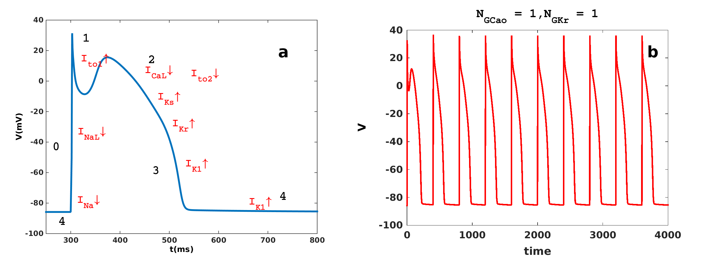
Figure 1: (a) Plot of the transmembrane potential $V$ versus time, for the HRD canine-ventricular model cell, showing the shape of the action potential (AP) and the major currents responsible for each phase of this AP. (b) Plots of these APs versus time for repeated pacing of a single cell, with fixed (representative) values of $G_{Kr}$ and of $\gamma_{Cao}$ (see the text and compare with Fig. 2 for the human-myocyte TP06 model).

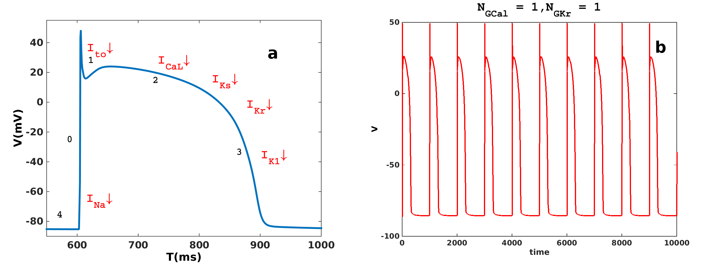
Figure 2: (a) Plot of the transmembrane potential $V$ versus time, for the TP06 human-ventricular model cell, showing the shape of the action potential (AP) and the major currents responsible for each phase of this AP. (b) Plots of these APs versus time for repeated pacing of a single cell, with fixed (representative) values of $G_{Kr}$ and of $G_{CaL}$ (see text and compare with Fig. 1 for the canine-myocyte HRD model).

We depict in Fig. 1 the shape of the action potential AP for the HRD canine-myocyte model, showing its different phases along with the major currents responsible for each stage. This figure also shows, for a representative set of values for $G_{Kr}$ and $\gamma_{Cao}$, the APs that we obtain with continuous pacing of the myocyte. We show for comparison, in Fig. 2, similar plots for the TP06 human-myocyte model.

Our 2D simulation domain, for the HRD model, is a square tissue with size $8.32$ cm $\times 8.32$ cm. For our 3D simulation we use the processed Diffusion-Tensor Magnetic-Resonance Imaging (DTMRI) data for the canine-ventricular anatomy, which is freely available for academic purposes at the CMISS website
(https://www.cmiss.org/), the details of which are given in the Supplementary Material supplementary .

Fig. 3 shows the geometry of the domain in which we investigate scroll-wave dynamics.

We describe the S1-S2 proptocol, which we use to produce the initial scroll waves in the Supplementary Material supplementary .

Figure 3: The anatomical geometry that we have created for our simulations by using DTMRI data (see text) for the coordinate mesh for the canine heart. Our simulation domain is the lower part of the heart that comprises the ventricles and the septum.

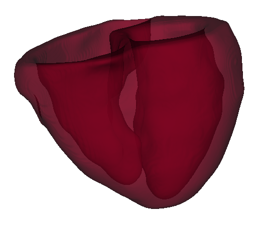
Figure 4: The anatomical geometry that we have created for our simulations of the TP06 human-ventricular model. We use the data for the coordinate mesh of the human heart that has been made available at Ref. humangeomdata . Our simulation domain is the lower part of the heart that comprises the ventricles and the septum.

For the HRD model, we investigate the effect on spiral- and scroll-wave dynamics of the following two currents.

(1) The L-Type Calcium current that is given by the equations

$$I_{CaL} = d^{p}\cdot f_{ca}\cdot f_{ca2}\cdot f\cdot{\bar{I}}_{CaL},$$ (1)

$${\bar{I}}_{CaL} = P_{Ca}\cdot z^{2}_{Ca}.\frac{(V_{m}-15.0).F^{2}}{RT}.$$ (3)

$$\frac{\gamma_{Cai}.[Ca]_{ss}\cdot\exp(\frac{z_{Ca}(V_{m}-15.0)F}{RT})-\gamma_{Cao}\cdot[Ca]_{o}}{\exp(\frac{z_{Ca}(V_{m}-15.0)F}{RT})-1},$$

where $d$, $p$, $f_{ca}$, $f_{ca2}$, and $f$ are gating variables; $P_{Ca}$ is the membrane permeability to the $Ca$ ion, in units of $cm/s$, and $z_{Ca}$ is the valence of the $Ca$ ion. The parameters $\gamma_{Cai}$ and $\gamma_{Cao}$ determine the magnitude and shape of the current $I_{CaL}$. They are the activity coefficient of the $Ca$ ion. We find that $\gamma_{Cao}$ has a stronger influence on the dynamics of the system than does $\gamma_{Cai}$. Therefore, we have chosen to study how the variation of $\gamma_{Cao}$, over a wide range, affects spiral- and scroll-wave dynamics in the HRD model.

(2) The delayed rectifier Potassium current is

$$I_{Kr} = \bar{G}_{Kr}\cdot X_{r}\cdot R_{Kr}\cdot(V_{m}-E_{Kr}),$$ (5)

$$\bar{G}_{Kr} = G_{Kr}\cdot\sqrt{\frac{[K^{+}]_{o}}{5.4}},$$ (6)

where $\bar{G}_{Kr}$ is the maximal conductance in units of $mS/\mu F$. $[K^{+}]_{o}$ is the extracellular concentration of $K^{+}$ ion in mmol/L . We study spiral- and scroll-wave dynamics in the HRD model for a wide range of values of $G_{Kr}$. The currents are given in units of $\mu A/\mu F$ .

In Eqs. LABEL:c3-icaleqn and  LABEL:c3-ikreqn, $G_{Kr}=0.01385423$ and $\gamma_{Cao}=0.341$; henceforth, we refer to these values as $GKR$ and $GCAO$, respectively. We investigate the dynamics of spiral waves in 2D tissue for 100 different cases, by varying $G_{Kr}$ as $GKR\times N_{GKr}$, where $N_{GKr}=1,2,...10$, and, simultaneously, varying $\gamma_{Cao}$ as $GCAO/N_{GCao}$, where $N_{GCao}=1,2...10$.

II.2 Human-Ventricular (TP06 Model) Simulations

For our DNSs of human-ventricular tissue, we use the TP06(tp06 ) model, which is a modified version of the TNNP model for human-ventricular cells tnnp04 ; this incorporates a total of $12$ ionic currents. The intracellular calcium handling in these models is not as detailed as it is in the HRD model.

The TP06 model uses 19 variables: (a) 1 for the transmembrane potential $V_{m}$, (b) 13 for ion-channel gates, namely, $m$, $h$, $j$, $d$, $f$, $f_{2}$, $f_{cass}$, $r$, $s$, $x_{s}$, $x_{r1}$, $x_{r2}$, and $\bar{R}$, and (c) 5 for intracellular, ion-concentration dynamics, namely, $Na_{i}$, $K_{i}$, $Ca_{i}$, $Ca_{sr}$, and $Ca_{ss}$.

As we have mentioned above, Fig. 2 gives the shape of the AP for this TP06 model; it depicts different, phases along with the major currents responsible for each phase; this figures also shows, for representative values of $G_{Kr}=GKR$ and $G_{CaL}=GCAL$, the APs with continuous pacing of the myocyte.

In Fig. 4 we have shown the anatomical geometry that we have created for our simulations by using the DTMRI data for the coordinate mesh of the human heart. This is the lower part of the heart that contains the ventricles and the septum.

The L-Type calcium current in the TP06 model is described by the following equations:

$$I_{CaL} = G_{CaL}.d.f.f_{Ca}\cdot 4\cdot{\frac{(V-15)F^{2}}{RT}}\cdot$$ (9)

$${\frac{0.25Ca_{SS}\exp({\frac{2(V-15)F}{RT}})-Ca_{o}}{\exp(\frac{2(V-F)F}{RT})-1}},$$

where $d$, $f_{ca}$, and $f$ are gating variables. The parameter $G_{CaL}$ determines the magnitude and shape of the current $I_{CaL}$. As in our work on the HRD model, we study how the variation of $G_{CaL}$, over a wide range, affects spiral- and scroll-wave dynamics in the TP06 model. Note that the variation of $G_{CaL}$ in the TP06 model corresponds to the variation of $\gamma_{Cao}$ in the HRD model.

In the TP06 model, the delayed rectifier Potassium current is

$$I_{Kr} = G_{Kr}{\sqrt{\frac{{K_{o}}}{5.4}}}.x_{r1}.x_{r2}.(V-E_{K}).$$ (10)

In our DNSs, we investigate $20$ different cases in 2D tissue: $G_{Kr}$ is taken as $G_{Kr}=GKR\times N_{GKr}$, where $GKR=0.153$, and $N_{GKr}=1,3,..7$. Along with this, $G_{CaL}$ is varied as $G_{CaL}=GCAL/N_{GCaL}$, where $GCAL=0.0000398$ and $N_{GCaL}=1,3,..9$. $GKR$ is the original value of $G_{Kr}$, as it appears in the model described by Eq. 10; likewise, $GCAL$ is the original value of $G_{CaL}$ as it appears in the model described by Eq. 9.

For our DNSs in the 3D anatomical geometry, we investigate 20 different cases as follows: $G_{Kr}=GKR\times N_{GKr}$, $N_{GKr}=1,3,...9$; and $\\ G_{CaL}=GCAL/N_{GCaL}$, $N_{GCaL}=1,3,...7$.

III Results

We present results from our simulations of the HRD model, at the cell level, in the Supplementary Material supplementary . The variations of the AP morphologies and APDR curves, for all the parameter values in our DNSs, are presented along with the plots of the currents $I_{Kr}$ and $I_{CaL}$. In this Section, we give results from our studies in 2D and then in 3D for the HRD model. Next we present the results of our simulations for the TP06 model.

It has been observed previously that the action potential duration restitution (APDR) is a crucial factor, which determines whether scroll waves or broken scroll waves develop in cardiac tissue fenton:02 ; garfinkel:00 ; koller:98 ; APDR1 ; APDR2 . The APDR is the shortening of the action potential duration(APD) as we increase the pacing frequency. A sharp APDR with a slope $>1$ in the APDR curve usually gives rise to a chaotic, broken-wave pattern. Another crucial determinant for the break up of spiral or scroll waves is early after depolarization (EAD), a premature re-excitation of the recovering tissue EAD1 ; Soling1 ; Soling2 . We examine a parameter region in the HRD model where we see neither EADs nor a sharp APDR curve (its slope is always $<1$).

III.1 2D Results

The conduction velocity $cv$ of a plane wave, passing from one end to the other end in our 2D simulation domain, is the same for all the cases we study; we find $cv=6.7002m/s$. By contrast, the wavelength $\lambda$ of the plane wave varies for each case; we define the wavelength to be the distance between the excited front and the $90\%$ recovered back end of the propagating plane wave of the transmembrane potential $V$ (before the initiation of the spiral wave). As we have noted above, we can also use the formula $\lambda=cv\times APD$, where APD is the action potential duration. We measure $\lambda$ for each of our parameter sets. The spiral wave, which we use as initial condition for our 2D DNSs, is created by using the S1-S2 protocol, which we describe in the Supplementary Material, supplementary , where we give representative pseudocolor plots of $V$ for plane-wave and spiral-wave initial conditions.

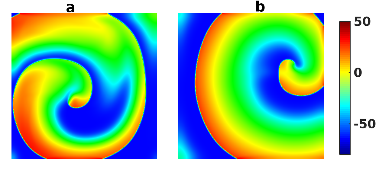
Figure 5: Pseudocolor plots of the transmembrane potential $V$ showing the two major types of spiral arms we observe in our 2D HRD-model simulations: (a) a spiral with a nonuniform wave width in different regions, with much thinner arms than in the center; and (b) a spiral with an almost uniform arm width. For the complete spatiotemporal evolution see the Videos S33 and S34 in the Supplementary Material supplementary .

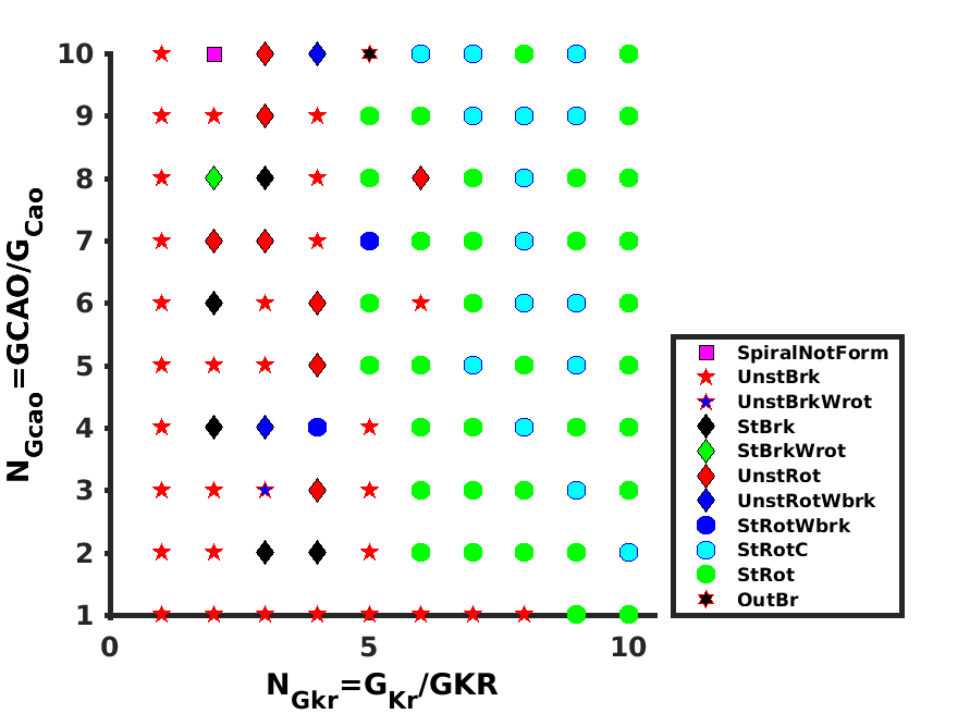
Figure 6: Phase diagram (or stability diagram) for the types of spiral-wave dynamics in our 2D domain for the HRD model. .The markers show the exact type of wave dynamics by using different shapes and colors. In the yellow region we obtain rotating spirals (${\mdblkcircle}$ with different colors); in the blue region we get broken spirals (★); and in the green region we see a mixed behavior, with transitions from unbroken spirals to states with broken spirals and vice-versa (diamond, ${\mdblkdiamond}$). In each region there is a statistically stable regime (waves remain in the medium without decaying) and an unstable regime (waves move away and disappear completely). In some cases, no spiral is formed (e.g., when $N_{GKr}=2,N_{GCao}=10$, denoted by a magenta square $\mdblksquare$). For $N_{GKr}=5$, $\gamma_{Cao}=10$, we see a far-field-break-up phenomenon (black-faced hexagon✶). The acronyms we use are as follows: SpiralNotForm- no spiral; UnstBrk - unstable break-up; UnstBrkWrot - unstable break-up state with rotating spiral states appearing temporarily; StBrk - stable break-up; StBrkWrot - stable break-up state with rotating spiral states appearing temporarily; UnstRot - unstable rotating spiral; UnstRotWbrk - unstable rotating spiral state with intermittent temporary spiral-break-up states; StRotWbrk - stable rotating spiral state with intermittent temporary spiral-break-up states; StRotC - stable rotating spiral state with temporary tiny break-up in the center; StRot - stable rotating spiral; OurBr - far-field break-up.

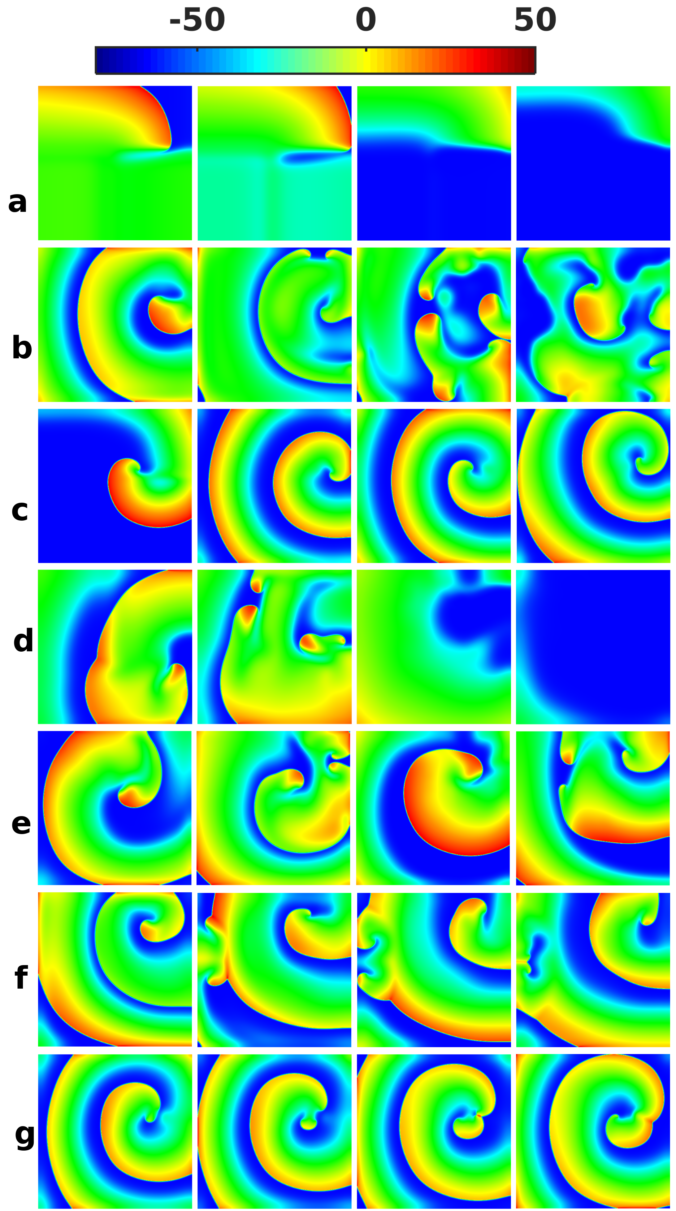
Figure 7: Pseudocolor plots of the transmembrane potential $V$ showing the different kinds of wave dynamics in our DNSs for the 2D-HRD model. The sub-panels, from the left to the right, show the evolution of the system at four different points of time (for the complete spatiotemporal evolution see the Videos S35, S36, S37, S38, S39, S310 and S311 in the Supplementary Material supplementary ). We observe the following seven types of spiral-wave dynamics (seven panels from the top to the bottom): (a) no spiral is formed ($N_{GKr}=2$, $N_{GCao}=10$); the waves disappear before evolving into a spiral (magenta square $\mdblksquare$ in Fig. 6); (b) a stable state with broken spirals ($N_{GKr}=2$, $N_{GCao}=6$), ($\mdblkdiamond$ in Fig. 6); the broken spirals interacts and regenerate themselves, without disappearing; (c) a stable single rotating spiral ($N_{GKr}=7$, $N_{GCao}=7$), (green bubbles $\mdblkcircle$ in Fig. 6); (d) an unstable break-up in which the broken waves quickly disappear($N_{GKr}=1,N_{GCao}=1$), (red stars $\star$ in Fig. 6); (e) region where a spiral breaks, recombines, rotates, again breaks and so on (green diamond, ${\mdblkdiamond}$, in Fig. 6). (f) far-field break-up (observed for $N_{GKr}=5$ and $N_{GCao}=10$) [black-faced hexagon ✶ in Fig. 6]; (g) a spiral with a local, short-lived instability of its core (here, $N_{GKr}=5$ and $N_{GCao}=9$), in the stable-rotating region [in Fig. 6 the cyan colored bubbles ${\mdblkcircle}$].

Given the range of parameter values we use, the initial spiral state shows rich and varied spatiotemporal evolution. Here, we give a detailed description of the various kinds of spiral-wave evolutions that we observe in the large parameter space we investigate.

We observe two (main) kinds of spiral arms, which we show in Fig. 5: (1) The first is a spiral with nonuniform arm widths at different regions in the simulation domain; these regions can have inherent instabilities, which cause spiral-arm thinning (but not enough to lead to the breaking up of the spiral-arm). They are stable and preserve their shape. The (average) wavelength of such a spiral wave is remarkably different from that of the plane wave from which it is formed. This kind of spiral arm is formed from plane waves of large width (as we find for low values of $G_{Kr}$ and high values of $\gamma_{Cao}$). (2) A spiral with almost uniform arm width. These spirals, which are stable and retain their uniform arm-width, are formed from small-width plane waves (as we find for high values of $G_{Kr}$ and low values of $\gamma_{Cao}$). Here, the spiral wavelength is comparable to that of the plane wave.

In summary, the spirals that form, in the different parameter regimes in the HRD model, have different sizes and shapes, even though they might evolve in a roughly similar manner to the final state and be characterized by generic terms such as spiral break up or spiral rotation. In Fig. 6 we give a phase diagram (or stability diagram) in the $N_{GKr}-N_{GCao}$ plane. [Recall that $G_{Kr}=GKR\times N_{GKr}$, where $N_{GKr}=1,2,...10$, and $\gamma_{Cao}=GCAO/N_{GCao}$, where $N_{GCao}=1,2...10$.] For this diagram we have used the results from the $100$ different pairs of parameter values that we have studied in the 2D HRD model. lot. The $3$ main types of dynamics we can observe are: broken waves, combined broken and rotating waves, and rotating waves. In each region we see some parts that sustain stable waves, i.e., the waves stay in the medium; in some other parts there are unstable waves, i.e., they move away and disappear from the medium. They are shown with different markers in each colored region (details are given in the figure caption).

In the break-up region we see two different kinds of phenomena: waves breaking up from the spiral core (core break-up); or waves breaking from the outer arms (far-field break-up). The far-field break-up is weak because it does not spread all the way to the core.

In Fig. 7 we show pseudocolor plots of $V$, from different stages of the spiral-wave evolution, going from left to right, for each of the different kinds of wave dynamics. The time-evolution of the spiral waves in the parameter-space we study is of the following seven major types (shown in the seven rows of Fig. 7): (a) No spiral wave is formed ($N_{GKr}=2$, $N_{GCao}=10$); the waves disappear from the medium before evolving into a spiral [magenta square $\mdblksquare$ in Fig. 6]. (b) A stable state with broken spirals is obtained ($N_{GKr}=2$, $N_{GCao}=6$) [$\mdblkdiamond$ in Fig. 6]; the broken spirals interact and regenerate themselves, without disappearing. (c) A stable single rotating spiral is formed ($N_{GKr}=7$, $N_{GCao}=7$) [green bubbles $\mdblkcircle$ in Fig. 6]. (d) There is unstable break-up in which the broken waves quickly disappear (e.g., for $N_{GKr}=1,N_{GCao}=1$) [red stars $\star$ in Fig. 6].(e) A region where a spiral breaks, recombines, rotates, again breaks and so on (green diamond, ${\mdblkdiamond}$, in Fig. 6). (f) There is far-field break-up (observed for $N_{GKr}=5$ and $N_{GCao}=10$) [black-faced hexagon ✶ in Fig. 6]. (g) There is an instability in the core region, exhibited by some parameter-combinations in the stable-rotating region (here, $N_{GKr}=5$ and $N_{GCao}=10$) [in Fig. 6 the regions marked by cyan colored bubbles ${\mdblkcircle}$]; such a core-break-up does not last, for the spiral core quickly regenerates itself; this has no far-reaching effect on the evolution of the spiral wave.

As we have mentioned earlier, the parameter region that we investigate in the HRD model leads to spiral-wave dynamics that does not obey the restitution hypothesis. According to this restitution hypothesis, if the slope of the APDR curves is $>1$, the spirals break up; if the slope is $<1$, the spirals do not break up. In our studies, the APDR slopes are always $<0.25$, yet we see spiral breakup. However, we see a correlation between the maximal slopes of the APDR restitution curves and the spiral-wave dynamics. The region where we obtain stable rotating spiral wave dynamics corresponds to the lower-right region of the APDR curves supplementary ; this is where the slopes are smallest, for the APDR curve is flat. The APD gets smaller and smaller in this region. Small values of the APD corresponds to small wavelengths $\lambda$. Such waves, with small widths, are not very prone to break-up in the HRD model.

III.1.1 Dominant frequencies

In this Subsection we examine the dominant frequencies of the spiral waves that are formed in our 2D simulations of the HRD model. For this we use the time series of the transmembrane potential $V$ from a few different sites in the simulation domain. The power spectra of these time series yield the dominant frequencies.

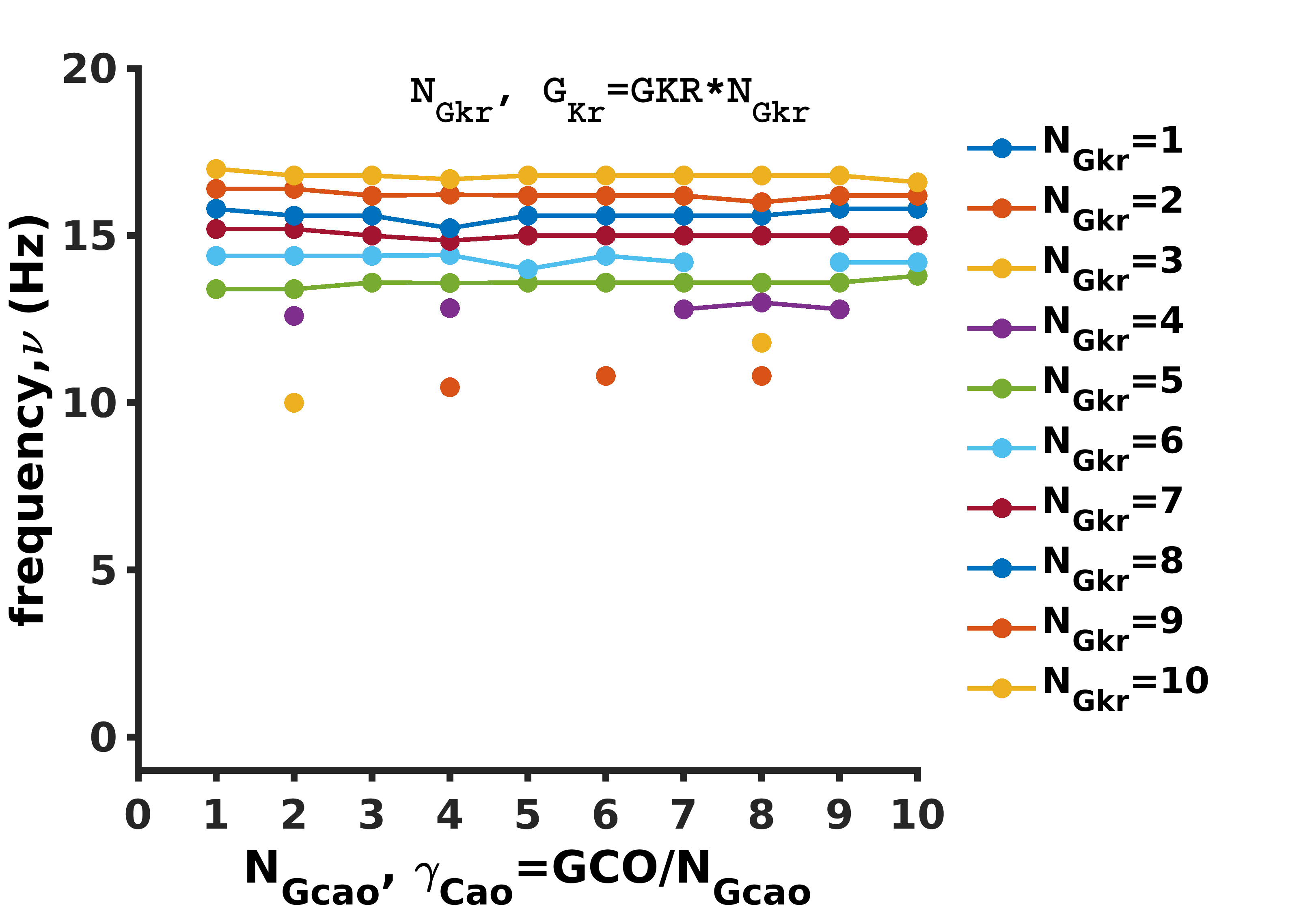
Figure 8: The dominant frequencies that we obtain from power spectra for all our parameter values, i.e., for $N_{GKr}=1,2..10$ and $N_{GCao}=1,2..10$. In the region where stable rotating waves exist, we see a prominent frequency in the spectrum. If the waves are unstable and disappear, it is not possible to identify a major frequency; the missing parameter values in this plot correspond to these unstable regions.

In Fig. 8 we show the dominant frequencies that we obtain from power spectra for all our parameter values, i.e., for $N_{GKr}=1,2..10$ and $N_{GCao}=1,2..10$. ( We give the spectra corresponding to these different wave dynamics in the Supplementary Material supplementary .) In the region where stable rotating waves exist, we see a prominent frequency in the spectrum. If the waves are unstable and disappear, it is not possible to identify a major frequency; the missing parameter values in this plot correspond to these unstable regions. Note that the frequency of the rotating wave increases as we increase $G_{Kr}$. The variation of $\gamma_{Cao}$ does not affect the dominant frequency substantially, as is evident from Fig. 8, where the curves are almost flat.

III.2 Three-dimensional (3D) Results

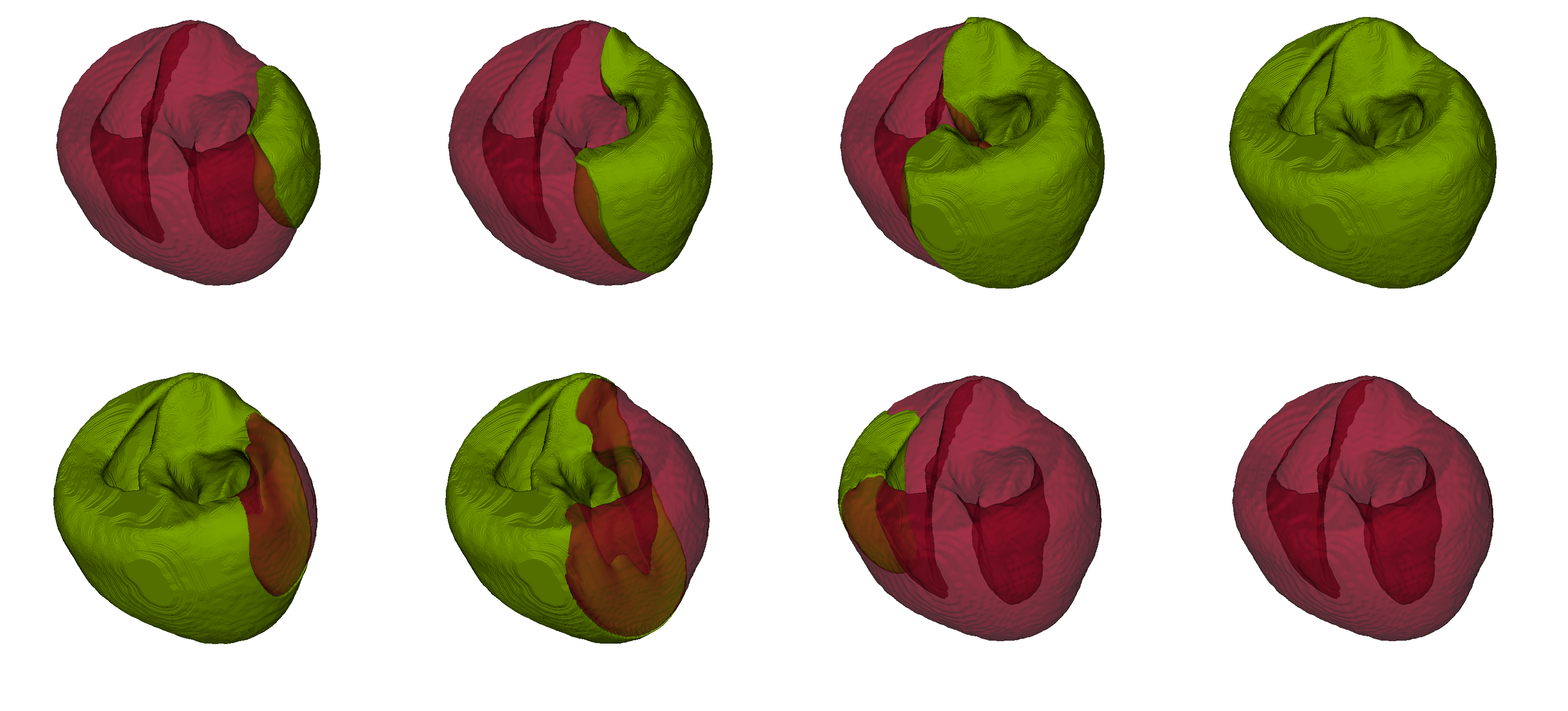
Figure 9: Two-level isosurface plots of $V$ for the HRD model illustrating a wave passing from one end to the other of our anatomically realistic simulation domain geometry under normal conditions and without any obstacles. The upper panels show the initial stages, time increasing from left to right; and the lower panels show the wave finally disappearing from the domain. For the complete spatiotemporal evolution see the Video S12 in the Supplementary Material supplementary .

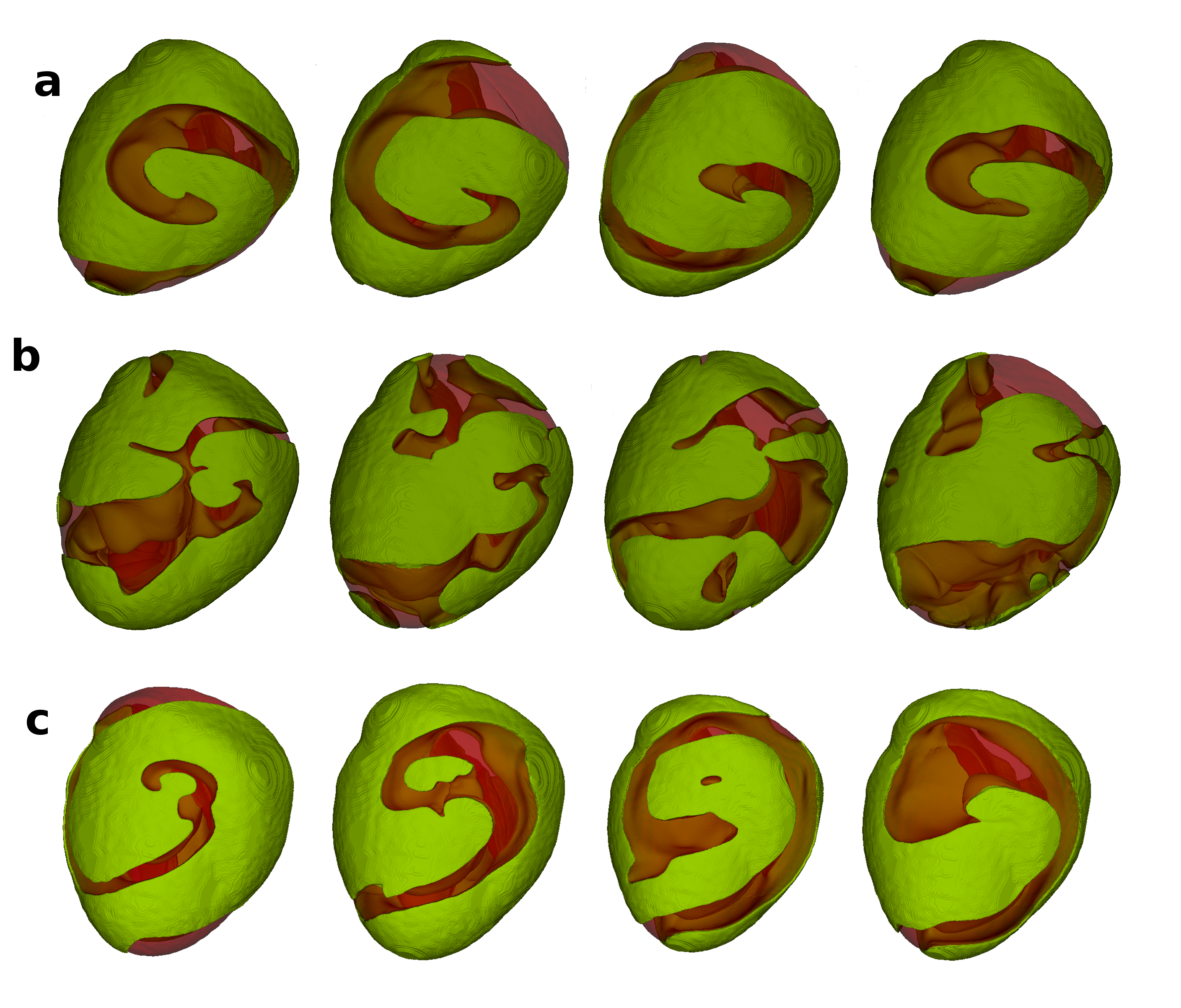
Figure 10: Two-level isosurface plots of $V$ illustrating the following: (a) A scroll wave in the stable rotating state; it rotates with a slightly meandering core, without breaking up ($N_{GKr}=7;N_{GCao}=7$). (b) A meandering scroll wave breaks up and spreads through the domain leading to a statistically stable chaotic state, for the representative parameter set $N_{GKr}=1,\,N_{GCao}=1$. (c) A scroll wave breaking while its central region passes through the right ventricle; this broken part quickly recombines and continues as a rotating stable wave, thus showing that such anatomical structures have only short-term effects on the wave dynamics (here, $N_{GKr}=7;N_{GCao}=3$). For the complete spatiotemporal evolution, see Videos S13, S14 and S15 in the Supplementary Material supplementary .

We now present our results on scroll-wave dynamics from our DNSs of the HRD model on the realistic canine-heart geometry that we have described above.

In Fig. 9 we show different stages of the spatiotemporal evolution of a plane wave passing through our anatomically realistic simulation domain, from one end to the other end (here there are no obstacles). The lower panels show how the wave moves and finally disappears. After a plane wave has passed through this domain, we apply the S1-S2 cross-field stimulus to produce a scroll filament in the middle of the domain supplementary . We then vary the parameters $G_{Kr}$ and $\gamma_{Cao}$ simultaneously and examine the effect of this change on development of the scroll wave for $3$s in real time.

With the original parameters of the HRD model, we see that the scroll wave immediately breaks up and develops into a spatiotemporally chaotic state. Within the time duration of our DNS, these broken scroll waves continue to spread in the domain, interact, recombine, and break up without disappearing; so the broken-wave state is statistically steady. The dynamics of broken scrolls for the parameters $G_{Kr}=GKR$ and $\gamma_{Cao}=GCAO$ is shown in Fig. 10(b). If we decrease $\gamma_{Cao}=GCAO/N_{GCao},$ by using $N_{GCao}=3,5,7$, the spatiotemporal evolution of scroll waves is qualitatively similar, with wave breaks and spatiotemporally chaotic behavior; but, for $N_{GCao}=3$ and $7$, the waves are unstable, they meander, break up, and finally disappear. This behavior is not visible for $N_{GCao}=1$ and $5$. Now we increase $G_{Kr}$ by factors of $3,\,5$, and $7$. In each case we vary $\gamma_{Cao}$ as above. Thus, we examine scroll-wave dynamics for $4\times 4=16$ parameter sets.

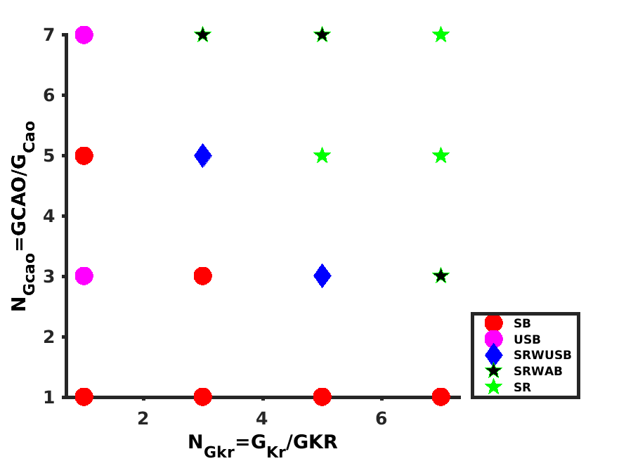
Figure 11: Phase diagram (or stability diagram) of scroll-wave dynamics in the HRD model, in the 3D anatomically realistic geometry for a canine heart, and in the $N_{GKr}-N_{GCao}$ plane, with $G_{Kr}=GKR\times N_{GKr}$ and $\gamma_{Cao}=GCAO/N_{GCao}$. We use markers: a circle ($\mdblkcircle$) indicates scroll-wave break up; a star ($\medblackstar$) indicates a rotating scroll wave; and a diamond ($\mdblkdiamond$) indicates a rotating scroll with transient break-ups, in between (SRWUSB - Stable Rotation With Unstable Breakup). The red circles indicate stable break-up (SB) and the magenta ones unstable break-up (USB). In the rotating-scroll region, the green star indicates stable rotating scrolls (SR), the black star indicates a short-term anatomical break-up, which quickly recombines and continues as a rotating stable wave (SRWAB - Stable Rotation With Anatomical Breakup) as shown in Fig. 10(c).

The different kinds of scroll-wave developments that we observe in our DNSs of the 3D HRD model in the anatomically realistic domain are depicted in Fig. 10: In Fig. 10(a) we show the development of a rotating scroll wave, with meandering, but without break up for a representative parameter set ($N_{GKr}=7$ and $N_{GCao}=7$). In Figs. 10(b) and (c) we show, respectively, how a meandering scroll wave breaks up and spreads through the domain and how a scroll wave breaks while its central region passes through the right ventricle, but such a break-up goes away very soon, in a time $\simeq 100ms$, and the wave recombines. We see this anatomical break-up arising solely because of the geometry rather than from functional break-up associated with parameter dependence. This anatomical break-up duration is negligible; it does not have a significant impact on the long-term behavior of scroll-wave dynamics.

The regions of stability of these different scroll-wave behaviors are depicted in a phase diagram in Fig. 11 (see the figure caption for details). Observe that, as we move to the right and upper regions of this phase diagram, scroll waves tend to be stable and rotating; they do not break up to form a chaotic state. This region corresponds to $N_{GKr}=7,5$ and $N_{GCao}=3,5,7$, and also $N_{GKr}=3$ and $N_{GCao}=5,7$. And anatomical breakup of scroll waves plays no significant role in the long-term dynamics of the system. Here also, as in our study of the 2D HRD model, we obtain stable rotating scroll waves in the bottom-right region of the APDR curves supplementary , where the APDR curve is nearly flat.

III.2.1 Dominant frequencies

We now examine, as we did in 2D, the dominant frequencies of the scroll waves that form in our DNSs of the 3D HRD model in the anatomical heart geometry. We use time series of the transmembrane potential $V$ from a few different sites from the simulation domain. In the Supplementary Material supplementary we present two-level isosurface plots of $V$ (left panel) showing different examples of scroll-wave dynamics and the corresponding power spectra (middle panel) of the time series (right panel) of $V$ from a representative point in the domain.

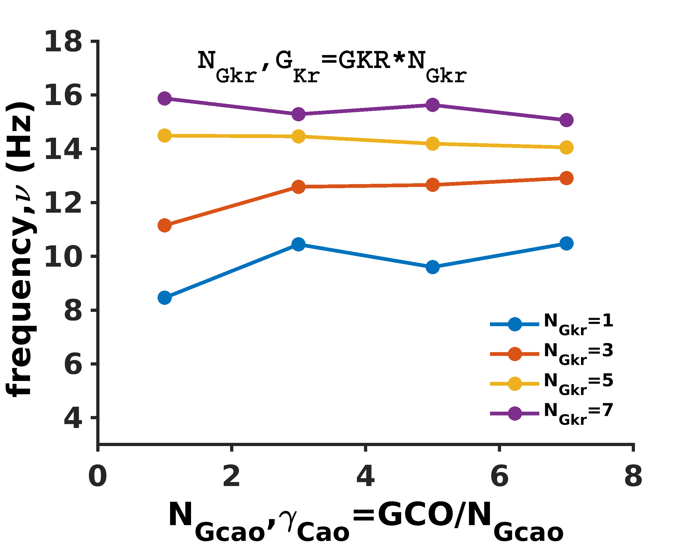
Figure 12: The dominant frequencies that we obtain from power spectra for all our parameter values, i.e., for $N_{GKr}=1,2..7$ and $N_{GCao}=1,2..7$. In the region where stable rotating waves exist, we see a prominent frequency in the spectrum. If the waves are unstable and disappear, it is not possible to identify a major frequency.

In Fig. 12 we plot the dominant frequencies that we obtain from power spectra (see the Supplementary Material supplementary ), for $N_{GKr}=1,2..7$ and $N_{GCao}=1,2..7$. In the region where a stable rotating scroll wave exists, we see a prominent frequency in the spectrum. If the waves are unstable and disappear, it is not possible to identify a major frequency. Here also, as in the 2D case, the dominant frequency increases as $G_{Kr}$ increases; and it is not affected significantly by a variation of $\gamma_{Cao}$.

IV Human-Heart (TP06) Model

We repeat the whole procedure described above on a human-heart geometry, with fiber orientation, by using the TP06 human-ventricular model. Our goal is to compare these results with their HRD-model counterparts. We present our results in two subsections, from 2D and 3D simulations. The shapes of the action potential (AP) and the APD-restitution (APDR) curves, for $5$ representative cases for the rapid rectifier current $I_{Kr}$, the Calcium current $I_{CaL}$,and different values of $G_{CaL}$ and $G_{Kr}$, for the TP06 model, are given in the Supplementary Material supplementary .

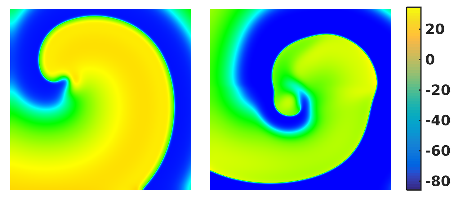
Figure 13: Pseudocolor plots of the transmembrane potential $V$ showing the two major types of spiral arms we observe in our 2D TP06-model simulations. Left panel: a spiral with an almost uniform arm width. Right panel: a spiral with a nonuniform wave width in different regions, with thin arms in some regions; (cf. Fig. 5 for the HRD model). For the complete spatiotemporal evolution see the Videos S16, S17 in the Supplementary Material supplementary .

IV.1 2D Results

For our simulations of the 2D TP06 model, we follow the same methods, numerical schemes, and initial spiral conditions we have used in our HRD-model DNSs. The conduction velocity of a plane wave passing from one end to the other end in the 2D domain is the same for all the cases, which is $6.960m/s$ for the TP06 model. We have measured the wavelength of the plane As we have described in Sec.I, we vary $G_{Kr}=GKR\times N_{GKr}$ and $G_{CaL}=GCaL/N_{GCaL}$ to obtain a total of $20$ different cases.

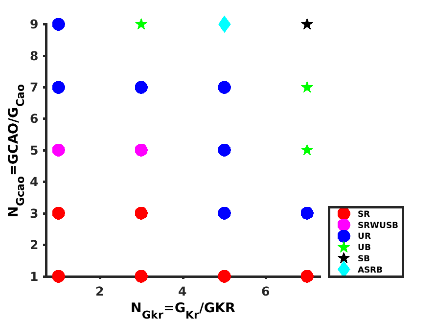
Figure 14: Phase diagram (or stability diagram) in the $N_{GKr}-N_{GCaL}$ plane for the types of spiral-wave dynamics in the 2D TP06 model, for the region of parameter space in our study. There are regions of broken-spiral states, rotating-spiral states, unstable-rotating states, and a mixed state. Different markers distinguish the following: Stable rotating spirals are denoted by bubbles (${\mdblkcircle}$) with different face colors; we see broken spirals (★), and unstable rotation (blue bubble). At one parameter value, denoted by a diamond ($\mdblkdiamond$), we see an alternating state, in which the wave undergoes a transition from a spiral to a broken-wave state and then recombines into a spiral again; this alternation continues for the duration of our DNS. In each region we see (a) stable states, in which the waves persist in the domain, and (b) unstable states, in which the waves move away and disappear completely from the domain. We define the following acronyms: SR - stable rotating; SRWUSB - stable rotating with unstable break-up in between; ASRB - alternating stable-rotating and breaking states; UR - unstable rotation; UB - unstable break-up; and SB - stable break-up (cf. Fig. 6 for the 2D HRD model).

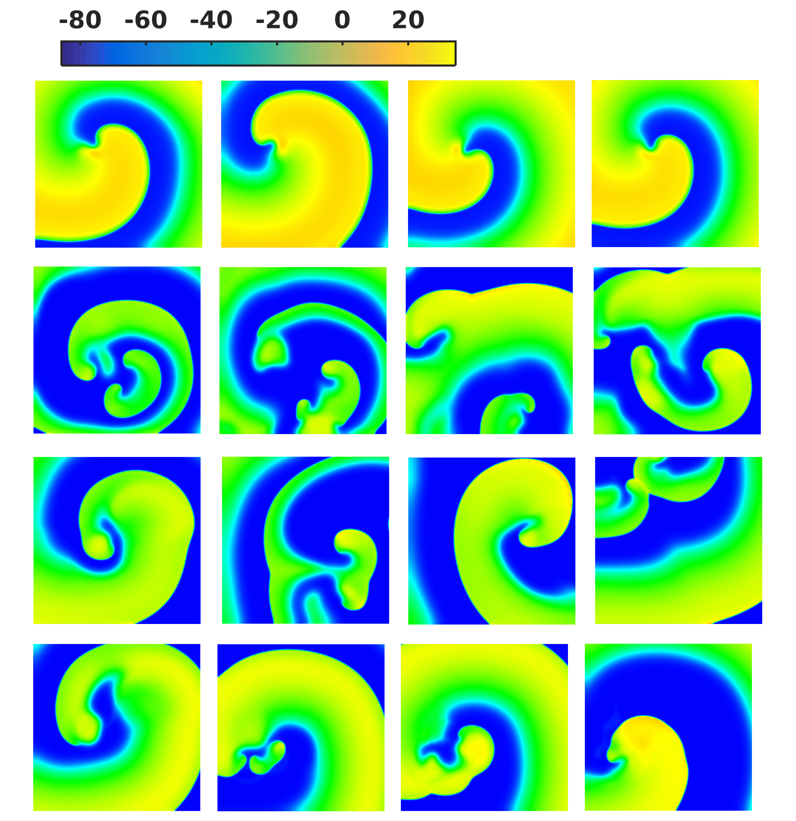
Figure 15: Pseudocolor plots of $V$ illustrating the four different kinds of spiral-wave dynamics that we observe in our DNSs for the 2D TP06 model. (for the complete spatiotemporal evolution see the Videos S18, S19, S20 and S21 in the Supplementary Material supplementary ): (a) A stable, single rotating spiral state (here, $N_{GKr}=1$, $N_{GCaL}=3$); red bubbles($\mdblkcircle$)in the phase diagram Fig. 14. (b) A stable state with broken spirals (here, $N_{GKr}=7$, $N_{GCaL}=9$); a black star ($\star$) in Fig. 14. (c) Alternating rotating and broken-wave states (here, $N_{GKr}=5$ and $N_{GCaL}=9$); in Fig. 14 a cyan diamond,${\mdblkdiamond}$. (d) The central spiral core shows an instability and a tendency to break up; such break-ups are transients, for the center quickly regenerates itself; this has no far-reaching effect on the evolution of spiral wave and it remains as a localized, isolated event at the center; magenta bubbles (${\mdblkcircle}$) in Fig. 14 (cf. Fig. 7 for the 2D HRD model).

We now describe the types of spiral-wave dynamics that we obtain in the large parameter space we have studied in the 2D TP06 model. As in the canine 2D HRD model (Fig. 5 in Sec.III.1), we observe two types of spiral arms. We depict these in Fig. 13.

In Fig. 14 we give the phase diagram (or stability diagram) for the different types of spiral-wave dynamics we obtain in the 2D TP06, for the $20$ cases that we have studied. The $3$ main colors in this phase diagram denote broken waves, a phase with both broken and rotating spirals, and rotating waves. In each region, we find that some waves are stable (they repeat themselves in time and do not move away from the domain), whereas others are unstable (they move away and disappear from the domain); these waves are shown with different markers in each coloured region. As we go from left to right in this phase diagram, the meandering of the wave increases, so it is prone to break up; eventually, for high values of $G_{Kr}$, the wave does break up. [Figure 14 is the counterpart of Fig. 6 for the HRD model.]

In Fig. 15 we show the different kinds of spiral-wave dynamics that we observe in our DNSs for the 2D TP06 model. The panels from the left to the right represent the evolution of the system at four different points of time. We observe the following four types of spiral-wave dynamics. (a) A stable, single rotating spiral state (for $N_{GKr}=1$, $N_{GCaL}=3$); stable spiral states are represented by red bubbles ($\mdblkcircle$) in the phase diagram of Fig. 14. (b) A stable state with broken spirals (here, $N_{GKr}=7$, $N_{GCaL}=9$); the broken spirals interact with each other, regenerates themselves, and do not leave the domain. This is denoted by a black star ($\star$) in Fig. 14. (c) We see alternately rotating and breaking spirals (here, for $N_{GKr}=5$ and $N_{GCaL}=9$); in Fig. 14, a cyan diamond,${\mdblkdiamond}$. (d) In some parts of the stable-rotating-wave region (green regime in Fig. 14), some of the spiral cores show a tendency to break and recombine in a very short interval of time. This instability of the core does not affect the long-term stability and dynamics of the spiral; the spiral core quickly reassembles and continues to rotate (see Fig. 15(d)), and remains as a localized, isolated event at the center; the regions in which we observe this are marked by magenta bubbles (${\mdblkcircle}$) in Fig. 14. In addition to the states mentioned above, we find unstable rotating states, for parameters denoted by blue bubbles, and unstable broken spiral waves, for parameters marked as green stars, in the phase diagram Fig. 14. These states last only for a short duration and quickly move away from the domain. [Figure 15 is the counterpart of Fig. 7 for the HRD model.]

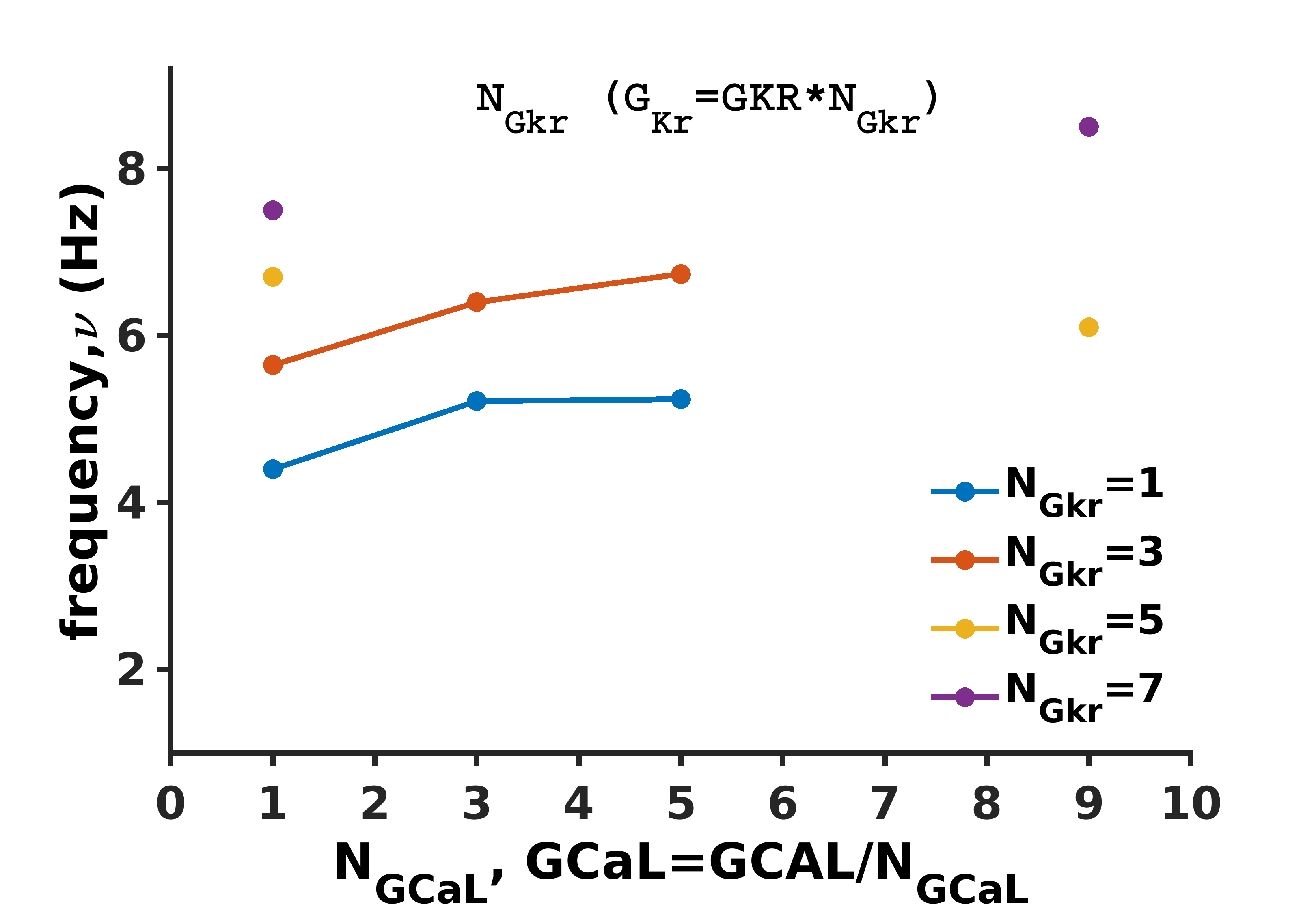
Figure 16: The dominant frequencies that we obtain from power spectra for all our parameter values (plots versus $N_{GCaL}$ for all the parameter values; $N_{GKr}=1,3..7$ and $N_{GCaL}=1,3..9$). In the region where stable rotating waves exist, we see a prominent frequency in the spectrum. If the waves are unstable and disappear, it is not possible to identify a major frequency; the missing parameter values in this plot correspond to these unstable regions (cf. Fig. 8 for the 2D HRD model).

IV.1.1 Dominant frequencies

In this Subsection we examine the dominant frequencies of the spiral waves formed in our 2D TP06 simulations. As we did in our study of the HRD model, we identify these frequencies from the power spectra of the time series of the transmembrane potential $V$, which we obtain from a few different points in the simulation domain.

In Fig. 16 we portray the most dominant frequencies that we observe for each of the parameter values. The figure is discontinuous in the unstable regions because the unstable regions do not sustain a wave. In the regions where the spiral has a well-defined peak frequency, the frequency increases as we move to high values of $G_{Kr}$; by contrast, $G_{CaL}$ has a very mild effect on the dominant frequency. A few examples of wave dynamics, along with the corresponding power spectra and the time series of $V$, are shown in the Supplementary Material supplementary .

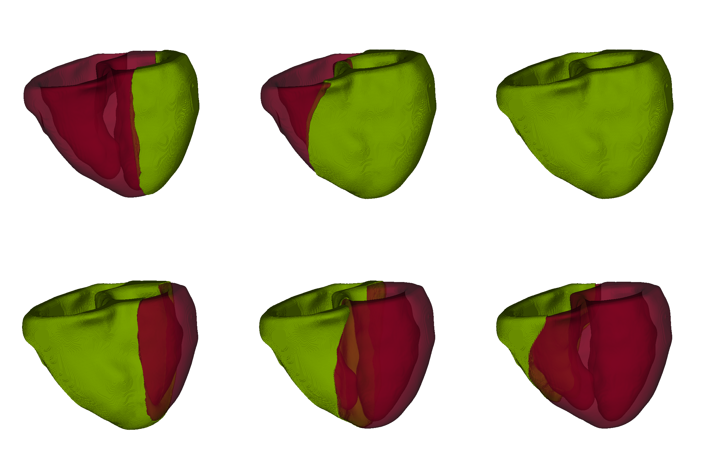
Figure 17: Two-level isosurface plots of $V$ for the 3D TP06 model illustrating a wave passing from one end to the other of our 3D realistic, human-heart geometry in the normal situation (without any obstacles). The upper panels show the initial stages from left to right; the lower panels show the wave finally moving out of the medium (cf. Fig. 9 for the 3D HRD model). For the complete spatiotemporal evolution see the Videos S22 in the Supplementary Material supplementary .

IV.2 3D Results

We now present our results from our DNSs of the TP06 model in a realistic, human-heart geometry that is reconstructed from DTMRI data (see Fig. 4).

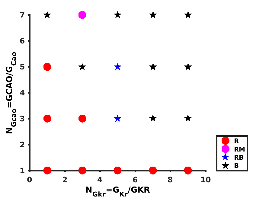
Figure 18: The phase diagram for scroll-wave dynamics in 3D TP06 model in a realistic, human-heart geometry. This diagram uses markers in the $N_{GKr}-N_{GCaL}$ parameter space. In general, a bubble indicates a rotating scroll wave and a star indicates scroll break-up. The red circles indicate stable rotation (R) and the magenta circle indicates a highly meandering rotating scroll (RM). The blue stars indicate a rotating scroll, which breaks up eventually (RB); and the black stars indicates stable break-up (B). All phases are stable states here, i.e., the waves do not disappear from the medium (cf. Fig. 11 for the 3D HRD model).

In the normal situation, a plane wave passes from one end to the other end of this geometry (without any obstacle). Figure 17 shows different stages of such a passing of a plane wave through the human-ventricular geometry. The upper panels show the initial stages; and the lower panels show the final stages when the wave finally moves away from the domain.

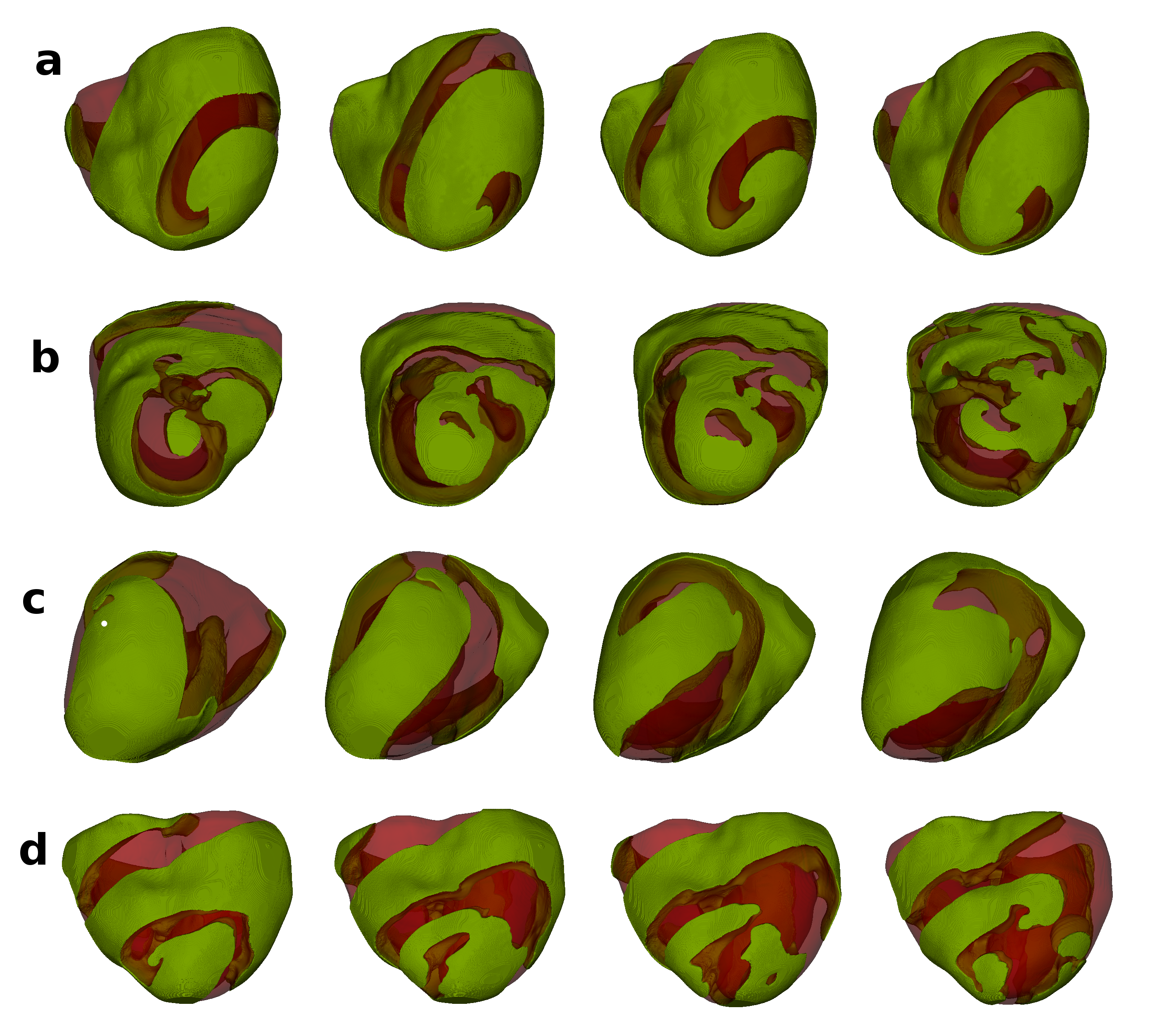
Figure 19: Representative figures showing each of the four types of scroll wave dynamics we observe in our system. The panels from left to right show, via two-level isosurface plots of $V$, the spatiotemporal evolution of the scrolls. (a) A stable rotating state where the scroll wave rotates and slightly meanders, without breaking up ($N_{GKr}=5,N_{GCaL}=1$). (b) A stable chaotic state where a scroll wave breaks up and the broken scrolls spread throughout the medium ($N_{GKr}=7,N_{GCaL}=3$). (c) A scroll wave meandering throughout the medium ($N_{GKr}=3,N_{GCaL}=7$). (d) A scroll wave rotates for a long while and eventually breaks up ($N_{GKr}=3,N_{GCaL}=3$); (cf. Fig. 10 for the 3D HRD model). For the complete spatiotemporal evolution see the Videos S23, S24, S25 and S26 in the Supplementary Material supplementary .

We follow the same procedure that we have used above for the HRD canine-ventricular model to initiate a scroll wave. Then, as in the HRD case, we vary the parameters $G_{Kr}$ and $G_{CaL}$ simultaneously and investigate the effects of these changes on the scroll-wave development. We record this development for $2.5$ seconds in real time.

With the original parameters of the TP06 model, we see that the scroll wave rotates without breaking; and it is stable for a long time after its initiation. The dynamics of such a scroll, for the parameters $G_{Kr}=GKR$ and $G_{CaL}=GCAL$, is shown in Fig. 19a.

With a decrease of $G_{CaL}$ by factors of $3,\,5,$ and $7,$ the dynamics we observe is the same as above; a stable rotating wave is formed and it continues to rotate, with a small amount of meandering, but it does not break. We then increase $G_{Kr}$ by factors of $3,\,5,\,7,$ and $9$, while simultaneously varying $G_{CaL}$ as above. Thus, we examine $5\times 4=20$ parameter sets. We present the general results of the scroll-wave behaviors in the phase diagram (or stability diagram) of Fig. 18. We observe that, as we move to the right and upper region of this phase diagram, the scroll waves tend to break up. This region corresponds to $N_{GKr}=7,\,9$ and $N_{GCaL}=3,\,5$ and $7$, and also $N_{GKr}=5,N_{GCaL}=7$ and $N_{GKr}=3,N_{GCaL}=5$. [This is the counterpart of Fig. 11 for the 3D HRD model.]

Figure 19 shows the scroll wave’s time development for each type of dynamics that we observe: (a) shows a stable rotating scroll-wave; and (b) depicts a scroll wave breaking up and forming a chaotic state ($N_{GKr}=9,N_{GCaL}=5$). We observe another interesting case in the scroll-wave rotating-meandering region, for $G_{Kr}=3$ and $G_{CaL}=7$: the wave meanders widely, throughout the simulation geometry; this is shown in Fig. 19(c); (d) provides an example of the cases $N_{GKr}=5N_{GCaL}=3,5$, where the scroll-wave rotates for a long time, and finally breaks up after $\approx 2$s. [This is the counterpart of Fig. 10 for the 3D HRD model.]

By comparing these figures with their 3D-HRD-model counterparts, we can see that scroll-wave dynamics for the TP06 model is quite different from that in the HRD model (for corresponding parameter regions).

IV.2.1 Dominant frequencies

In this Subsection we examine the dominant frequencies of the scroll waves formed in the anatomical heart geometry by using the time series of the transmembrane potential from a few different sites of the domain.

Figure 20: The dominant frequencies we observe for all the parameter values; $N_{GKr}=1,2..9$ and $N_{GCaL}=1,2..7$. For stable states, the frequency increases with $G_{Kr}$; the variation with $G_{GaL}$ is either small or nonexistent.

Here also, as in the 2D case, the dominant frequency of the scroll wave increases with an increase in $G_{Kr}$; but this frequency is not affected significantly by the variation of $G_{CaL}$. This is shown in Fig. 20, where we show the dominant frequencies of the scrolls for the whole parameter space that we explore. A few examples of scroll-wave dynamics, along with the corresponding power spectra and the time series of $V$ for the 3D TP06 model, are given in the Supplementary Material supplementary .

V Conclusions

We have conducted extensive, in silico studies of the direct effects of two major, ion-channel conductances on spiral- and scroll-wave dynamics in idealised (2D) and anatomically detailed (3D) geometries for the canine- and human-ventricular models (HRD and TP06, respectively). We find that $I_{GKr}$ and $I_{GCaL}$ are two important currents that determine the characters of spiral- and scroll-wave dynamics, namely, rotation, meandering, or the break-up of these waves in the ventricles. The effects of changes in these currents, on such wave dynamics, are most clearly visible when they are changed together, rather than individually (specifically, when $G_{Kr}$ increases and $G_{CaL}$ decreases). We have observed this qualitative feature in the two distinctly different models, for two different mammalian species, namely the canine-ventricular HRD model and human-ventricular TP06 model.

The precise forms of the spiral or scroll wave that are formed in the simulation domain, in the absence of any parameter variation, are, of course, model specific. Hence, changes in these waves and their dynamics, as a function of model parameters, are also model specific. Nevertheless, there is a qualitative similarity in the transitions from one phase to another, the phase diagrams that we have presented for both HRD and TP06 models in both 2D and 3D. Details differ, of course, as we can see by comparing the phase diagrams for these models carefully. Such a detailed comparison between wave dynamics in these different mammalian models has not been attempted hitherto.

In our HRD model simulations, the scroll-wave break-up that we observe, without varying the values of $G_{Kr}$ and $G_{Cao}$, undergoes a transition to a stable meandering wave, without break up, as we vary the parameters. In the TP06 model simulations, we observe the reverse phenomenon, i.e., a transition occurs, from the stable rotating state, in the initial parameter region, to a broken-scroll or chaotic state (even though we vary parameters over a range that is similar to the one we use in our HRD-model simulations). In both these models, the combination of the ion-channel conductances, for $I_{Kr}$ and $I_{GCaL}$, plays a crucial role in determining the nature of scroll-wave dynamics. Recall that the parameter region we have explored is devoid of other commonly observed mechanisms that lead to uncontrolled scroll-wave behavior, such as a sharp APD restitution curve, early after depolarizations, and delayed after depolarizations.

There is no consensus on whether the geometric details of the heart itself affect scroll-wave dynamics or not; and, if they do, to what extent and in which way. We have observed, in our simulations with anatomically realistic geometries and fiber-orientation details, that the long-term effect of the geometry, without abnormal inhomogeneities or other variations, on scroll-wave dynamics is negligible. The role that the geometry itself plays here is to trap the re-entrant waves, preventing them from decaying at the boundaries and thus stabilizing them. The primary determining factors, which affect wave dynamics and transitions from one sort of dynamics to another, are the conductances that govern the values of $G_{Kr}$ and $G_{CaL}$.

We conclude that the chaotic dynamics of scroll waves is not only produced by the common causes like a sharp APDR, EADs, and DADs, but also by a combined variation of the rapid-rectifier and calcium currents, $I_{Kr}$ and $I_{CaL}$; these play a crucial role in determining the dynamics of spiral and scroll waves in the two mammalian-heart models that we have studied. Our detailed description of the dependence of spiral- and scroll-wave dynamics on changes in these currents should provide insights into an understanding of the effects of drugs that target these current channels.

We mention some limitations of our study. We have used a monodomain model for the cardiac tissue equations in our study; bidomain models are more realistic than monodomain ones; however, a recent study Potse has shown that the latter are adequate when currents are low, as in our study. To impose boundary conditions we have used a phase-field approach appndxphase ; this can also be done with a finite-element model. The dynamics of scroll waves is affected by a many more parameters than the two we study in detail. We have chosen these parameters for the reasons mentioned in this paper. A comprehensive study, including the simultaneous effects of change in more than two parameters, is computationally very expensive.

VI Acknowledgments

We thank Council of Scientific and Industrial Research, University Grants Commission and Department of Science and Technology (India) for support, and the Supercomputing Education and Research Centre (IISc) for computational resources.

References

- (1) J.M. Davidenko, Journal of Cardiovascular Electrophysiology 4 6, 730-746 (1993).
- (2) R. Clayton and A. Panfilov, Progress in Biophysics and Molecular Biology 96, 19-43 (2008).
- (3) R.H. Clayton, O. Bernus, E.M. Cherry, H. Dierckx, F.H. Fenton, L. Mirabella, A.V. Panfilov, F.B. Sachse, G. Seemann, H. Zhang, Progress in Biophysics and Molecular Biology 104 22-48 (2011).
- (4) N.A. Trayanova, Circ. Res. 108, 113-128 (2011).
- (5) E.M. Cherry and F.H. Fenton, New Journal of Physics 10 (2008) 125016 (43pp) (2008); doi:10.1088/1367-2630/10/12/125016 .
- (6) J. Keener , J. Sneyd, Mathematical Physiology (Springer, New York, 1998).
- (7) A. Pertsov and M. Vinson, Philosophical Transactions: Physical Sciences and Engineering 347 1685, 687-701 (1994).
- (8) J.N. Weiss, A. Garfinkel, et al. Journal of Molecular and Cellular Cardiology 82, (2015).
- (9) R. Majumder, A. R. Nayak, and R. Pandit, Heart Rate and Rhythm (Springer, 2011), pp. 269–282.
- (10) T.K. Shajahan, S. Sinha and R. Pandit, “The Mathematical Modelling of Inhomogeneities in Ventricular Tissue” in Complex Dynamics in Physiological Systems: From Heart to Brain. Understanding Complex Systems, Springer, Dordrecht, edited by S. K. Dana, P. K. Roy, J. Kurths, pp. 51-67, (2009).
- (11) R. Majumder, A. R. Nayak, and R. Pandit, PLoS ONE 7, e45040 (2012).
- (12) R. Majumder, A. R. Nayak, and R. Pandit, PLoS ONE. 6 4, e18052 (2011).
- (13) A. R. Nayak and R. Pandit, Frontiers in Physiology 5, 207 (2014).
- (14) A. R. Nayak, T. K. Shajahan, A. V. Panfilov, and R. Pandit, PLoS ONE. 8 9, e72950 (2013).
- (15) T. Ikeda, M. Yashima, T. Uchida, D. Hough, M. C. Fishbein et al., Circ. Res. 81, 753 (1997).
- (16) Z. Y. Lim, B. Maskara, F. Aguel, R. Emokpae Jr., and L. Tung, Circulation 114, 2113-2121 (2006).
- (17) T.K. Shajahan, S. Sinha, and R. Pandit, Phys. Rev. E. 75, 011929-1 - 011929-8 (2007).
- (18) T.K. Shajaha , A. R. Nayak, and R. Pandit, PLoS ONE. 4 3, e4738 (2009).
- (19) J. Christoph, M. Chebbok, C. Richter, et al. Nature 555, 667–672 (2018).
- (20) J. Grondin, D. Wang, C.S. Grubb, N. Trayanova, E.E. Konofagoua, Computers in Biology and Medicine 113, 103382 (2019).
- (21) Hund TJ, Rudy Y. Rate dependence and regulation of action potential and calcium transient in a canine cardiac ventricular cell model. Circulation. 2004 Nov 16; 110 (20):4008-74.
- (22) Online Data Supplement - Model of the canine cardiac ventricular cell, Hund and Rudy
- (23) A Dynamic Model of the Cardiac Ventricular Action Potential - Simulations of Ionic Currents and Concentration Changes, Luo, C. and Rudy, Y. , 1994, Circulation Research, 74, 1071-1097.
- (24) Fenton FH, Cherry EM, Hastings HM, et al. (2002) Multiple mechanisms of spiral wave breakup in a model of cardiac electrical activity. Chaos 12(3): 852.
- (25) Garfinkel A, Kim YH, Voroshilovsky O, et al. (2000) Preventing ventricular fibrillation by flattening cardiac restitution. PNAS 97(11): 6061.
- (26) Koller ML, Riccio MR, Gilmour RJ (1998) Dynamic restitution of action potential duration during electrical alterans and ventricular fibrillation. Am J Physiol Heart Circ Physiol 275: H1635.
- (27) Ten Tussher KHWJ, Panfilov AV, Cell model for efficient simulation of wave propagation in human ventricular tissue under normal and pathological conditions, Phys. Med. Biol. , 51:6141-6156
- (28) Stevens C, Remme E, LeGrice IJ, Hunter PJ, JBiomech.36:737-748 (2003).
- (29) F.H. Fenton, E.M. Cherry, A. Karma, and W.J. Rappel, CHAOS 15, 013502 (2005)
- (30) ten Tusscher KHWJ, Noble D, Noble PJ, and Panfilov AV (2004) A model for human ventricular tissue. Am J Physiol Heart Circ Physiol 286: H1573.
- (31) Shajahan TK, Nayak AR, Pandit R. Spiral-wave turbulence and its control in the presence of inhomogeneities in four mathematical models of cardiac tissue. PLoS One. 2009;4(3):e4738. doi:10.1371/journal.pone.0004738.
- (32) Qu, Z., Weiss, J. N., and Garfinkel, A. (1999). Cardiac electrical restitution properties and stability of reentrant spiral waves: a simulation study. Am. J. Physi. Heart Circ. Physiol. 276, H269–H283.
- (33) N. Vandersickel, I. Kazbanov, A. Nuitermans, L.D. Weisse, R. Pandit, and A.V. Panfilov. A Study of Early Afterdepolizations in a Model for Human Ventricular Tissue. doi:10.1371/journal.pone.0084595, (2014).
- (34) S. Zimik, N. Vandersickel, A.R. Nayak, A.V. Panfilov, and R. Pandit. A Comparative Study of Early Afterdepolarization-Mediated Fibrillation in Two Mathematical Models for Human Ventricular Cells. PLoS ONE, 10(6):e0130632, (2015).
- (35) S. Zimik, A.R. Nayak, and R. Pandit. A computational study of the factors influencing the pvc-triggering ability of a cluster of early afterdepolarization-capable myocytes. PLoS ONE, 10 (12):e0144979, (2015).
- (36) Online Supplemental Material: Spiral- and scroll-wave dynamics in mathematical models for canine and human ventricular tissue with varying Potassium and Calcium currents
- (37) M. Potse, B. Dube, J. Richer, A. Vinet and R. M. Gulrajanii “A Comparison of Monodomain and BidomainReaction-Diffusion Models for Action PotentialPropagation in the Human Heart” IEEE Transactions on Biomedical Engineering, 53 No. 12 (2006)
- (38) David E. Clapham, Calcium Signaling, Cell, Vol.80, 259-268, (1995).
- (39) Mines, G. R. , On dynamic equilibrium in the heart, J. Physiol. (London) 46: 349-382 (1913)
- (40) E. Braunwald , Heart Disease: A Textbook of Cardiovascular Medicine Vol.1, Sauders International Edition (Fourth Ed).
- (41) Kléber AG, Rudy Y (2004), Basic Mechanisms of Cardiac Impulse propagation and Associated Arrhythmias, Physiol. Rev.84 431-488
- (42) See Chapter 3, PhD Thesis (unpublished) of K.V. Rajany, Indian Institute of Science, Bangalore, India (2020).