Optimization in a non-linear Lanchester-type model
involving supply units

Abstract

In this paper, a non-linear Lanchester-type model involving supply units is introduced. The model describes a battle where the Blue party consisting of one armed force $B$ is fighting against the Red party. The Red party consists of $n$ armed forces each of which is supplied by a supply unit. A new variable called "fire allocation" is associated to the Blue force, reflecting its strategy during the battle. A problem of optimal fire allocation for Blue force is then studied. The optimal fire allocation of the Blue force allows that the number of Blue troops is always at its maximum. It is sought in the form of a piece-wise constant function of time with the help of "threatening rates" computed for each agent of the Red party. Numerical experiments are included to justify the theoretical results.

I Introduction

In 1916, Lanchester (Lan ) introduced a mathematical model for a battle in the form of a system of differential equations two unknowns of which are the number of the two involved parties. In 1962, Deitchman (Dei ) extended Lanchester’s model by investigating battle between an army and a guerilla force. This model is called a guerilla warfare model or an asymmetric model. In this model, the fire of guerilla force is supposed to be aimed while of the army is unaimed. Later, Schaffer (Sch ) and Schreiber (Sch1 ) generalized Deitchman’s model further by taking into account the intelligence and considered the problem of optimizing the fire allocation of the army. Recently, Kaplan, Kress and Szechtman (KKS) (Kap ,Kre ) also considered Lanchester model with intelligence in a scenario of counter-terrorism. In this asymmetric model, intelligence play a decisive role in the outcome of the combat. In addition, a lot of researchers are interested in optimization problems involving warfare models. In 1974, Taylor (Tay ) studied several problems of optimizing the fire allocation for some warfare models. Lin and Mackay (Mac ) extended Taylor’s results on optimization of fire allocation for Lanchester’s model of the form one against many. A common interest of these two studies is optimizing the number of troops. Feichtinger and his colleagues (Fei1 ) studied an optimization problem for KKS model with objective function being the cost of the battle, control variables being intelligence and reinforcement. In 2019, we investigated a modified asymmetric Lanchester $(n,1)$ model describing a combat between a group of $n$ counter-terrorism forces and a single group of terrorists, see (Manh ). In these works above, the role of military supply has not been studied thoroughly. In a combat, the victory of one party is not only decided by the armed forces but also by the supply units. In 2017, Kim and his colleagues (Kim ) considered a Lanchester’s model where one of the party is supported by a supply unit. Besides, there have been multi-party combats where a Blue force $B$ fights against $n$ independent forces of the Red party: $R^{1},R^{2},...,R^{n}$ and each of these forces is supported by one of $n$ different supply agents $A^{1},A^{2},...,A^{n}$. The supply units do not fights the Blue force directly. However, their supports for $R^{1},R^{2},...,R^{n}$ may affect both the progress and the outcome of a combat. One such combat is the civil war in Syria, starting in 2011. In order to investigate such war, we introduce a novel model of non-linear Lanchester’s type. In Lanchester’s model using system of differential equations, the rate of troops decreasing of a force is computed by attrition rate of its rival force multiplied by the rival’s number of troops. In our model, attrition rate of $R^{i}:\,i=1,2,...,n$ is assumed to be a linear function of the number of its supply unit and this supply unit can also be attrited by $B$. Let us recall that in classical non-linear Lanchester’s model, the supply units have not been taken into account but only the armed forces. Besides, in our model, a fire allocation is added to the Blue force. This distribution is used to express the strategy of $B$ during the conflict. The allocation is in the form of $2n$ non-negative number, whose sum equals to $1$, multiplied by $B$’s attrition rates with respect to $R^{i}$ and $A^{i}:\,i=1,..,n$. This allocation obviously has an impact on the dynamics of the system of differential equations and hence the progress and outcome of the combat. For this novel model, we consider the problem of optimal fire allocation for $B$, thus, we seek for fire allocation such that the remaining troops of $B$ at any time is maximum. The optimal fire allocation is derived using the so-called "threatening rates", which are computed for $R^{i}$ and $A^{i}:\,i=1,..,n$. Numerical experiments have justified the theoretical findings.
The rest of the paper is organized as follows. Section 2 is devoted to present model settings and to investigate the optimization problem for this model. Numerical experiments are presented in Section 3 to illustrate the theoretical results. Conclusion and some possible further developments are discussed in the last section.

II Main Results

II.1 The Model

Let us consider a combat between a Blue party and a Red party and assume that each agent of the Red party is supplied by a corresponding supply unit. We use the following notations:

• $B$: Blue force.

• $R^{i}(i=1,\ldots,n)$: $i$-th agent of the Red party.

• $A^{j}(j=1,\ldots,n)$: corresponding supply agents for $R^{j}$ forces.

• $r_{R^{i}}$: an attrition rate of $B$ to $R^{i}$.

• $r_{A^{j}}$: an attrition rate of $B$ to $A^{j}$.

• $f_{\alpha^{i}}$: an attrition function of $A_{i}$ complementing $R^{i}$ to $B$.

• $P=\left(p_{1},\ldots,p_{i},\ldots,p_{n},p_{n+1},\ldots,p_{n+j},\ldots,p_{2n}\right)$: the fire allocating proportion of $B$ to $R^{i}$ and $A^{j}\,(i,j=1,\ldots,n)$ respectively.

• $\alpha^{i}_{c}:$ the fully-connected attrition rate of $R^{i}$ with $A^{i}$.

• $\alpha^{i}_{d}:$ the fully-disconnected attrition rate of $R^{i}$ with $A^{i}$ $(\alpha^{i}_{d}\leq\alpha^{i}_{c})$.

We denote this model as $\left({B\texttt{ vs }((R^{1},A^{1}),\ldots,(R^{n},A^{n}))}\right).$ The diagram for this model is presented in Figure 1.

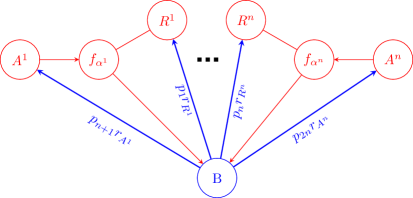
Figure 1: Diagram for the model $\left({B\texttt{ vs }((R^{1},A^{1}),\ldots,(R^{n},A^{n}))}\right).$

Let us consider the problem of finding the optimal fire allocation of $B$ such that at any time $t$, the remaining troops of $B$ is maximized. We seek for the optimal fire allocating proportion of $B$ in the form of a piece-wise constant function. This choice is realistic since it is absurd to alter the fire allocation constantly, especially during a certain stage of the battle. For this purpose, we assume that $P=\left(p_{1},\ldots,p_{n},p_{n+1},\ldots,p_{2n}\right)$ is a piece-wise constant proportion where $p_{1},\ldots,p_{2n}\in\left[{0;1}\right]:\,\sum\limits_{k=1}^{2n}p_{k}=1$ at any time $t$.

The attrition rates of $R^{i}$ to $B$ is supposed to be entirely dependent on its corresponding supply unit. Thus the complementing attrition functions are assumed to be linear ones of the form:

$$f_{\alpha^{i}} =\alpha_{d}^{i}+(\alpha_{c}^{i}-\alpha_{d}^{i})\frac{A^{i}}{A^{i}_{0}}:i=1,\ldots,n.$$

where $A^{i}_{0}$ number of $A^{i}$’s troops at the beginning. Let us observe that, at the beginning, when $A^{i}=A^{i}_{0}$, $R^{i}$ and $A^{i}$ has a full connection and $f_{\alpha^{i}}$ attains its maximal value $\alpha_{c}^{i}$. When $A^{i}$ is totally eliminated by $B$, $A^{i}=0$, the connetion between $R^{i}$ and $A^{i}$ is terminated and $f_{\alpha^{i}}$ is now only $\alpha_{d}^{i}$.

The numbers of troops of all the parties involved in the battle are governed by the following system of differential equations:

$$\begin{cases}\frac{dB}{dt}=-\sum\limits_{i=1}^{n}\left[\alpha_{d}^{i}+\left(\alpha_{c}^{i}-\alpha_{d}^{i}\right)\frac{A^{i}}{A_{0}^{i}}\right]R^{i},\\ \frac{dR^{i}}{dt}=-p_{i}r_{R^{i}}B:i=1,\ldots,n,\\ \frac{dA^{j}}{dt}=-p_{n+j}r_{A^{j}}B:j=1,\ldots,n.\end{cases}$$ (1)

It is apparent that supply agents $A^{1},\ldots,{A^{n}}$ create their impact on the outcome of the battle by influencing the attrition rate of $R^{1},\ldots,R^{n}$ to $B$. When their numbers of troops are reduced to zero, their impacts are stopped accordingly.

II.2 Optimal fire allocation of Blue force

For the model (1), we consider the problem of maximizing the Blue force’s number of troops at any time $t$. Let us compute the following:

$$b_{i} =\alpha_{c}^{i}r_{R^{i}}:i=1,\ldots,n,$$ (2)

$$b_{n+j} =\frac{r_{A^{j}}\left(\alpha_{c}^{j}-\alpha_{d}^{j}\right)R^{j}_{0}}{A_{0}^{j}}:j=1,\ldots,n.$$

We will refer to these numbers as "threatening rates". These rates represent the "threats" which $R^{1},\ldots,R^{n}$ forces and theirs supply agents expose to the Blue force. The optimal fire allocation of $B$ is pointed out in the following theorem.

Theorem 1.

Suppose that the optimal fire allocation $P^{*}$ is sought in the set $\mathcal{P}=\{P=(p_{1},\ldots,p_{n},p_{n+1},\ldots,p_{2n}):p_{k}\in[0,1]\text{ is constant }\forall k=1,\ldots,2n;\sum\limits_{k=1}^{2n}p_{k}=1\}$. Then the optimal fire allocation of $B$ is :
${P^{*}}=\left({0,...,0,\underbrace{1}_{k},0,...,0}\right)\,where\,\,k=\mathop{\arg\max}\limits_{l=1,...,2n}\left\{b_{l}\right\}.$

Proof.

Let $X(t)=\int_{0}^{t}B(s)ds$. It follows that $X^{\prime}(t)=B(t)$ and

$$X^{\prime\prime}(t)=B^{\prime}(t)=-\sum\limits_{i=1}^{n}\left[\alpha_{d}^{i}+\left(\alpha_{c}^{i}-\alpha_{d}^{i}\right)\frac{A^{i}}{A_{0}^{i}}\right]R^{i}.$$ (3)

We also have

$$\int_{0}^{t}dR^{1}=-\int_{0}^{t}p_{1}r_{R^{1}}B(s)ds\Rightarrow R^{1}(t)-R^{1}(0)=-p_{1}r_{R^{1}}X(t).$$

This leads to

$$R^{1}(t)=-p_{1}r_{R^{1}}X(t)+R^{1}_{0}.$$ (4)

By similar arguments, we get

$$R^{i}(t)=-p_{i}r_{R^{i}}X(t)+R^{i}_{0}:i=1,\ldots,n,$$ (5)

$$A^{j}(t)=-p_{n+j}r_{A^{j}}X(t)+A^{j}_{0}:j=1,\ldots,n.$$ (6)

Substituting (5), (6) into (3) we obtain

$$X^{\prime\prime}(t)=-C_{1}X^{2}(t)+C_{2}X(t)-C_{3},$$ (7)

where

$${C_{1}} =\sum\limits_{i=1}^{n}{\frac{{p_{i}{p_{n+i}}{r_{R^{i}}}{r_{{A^{i}}}}\left({\alpha_{c}^{i}-\alpha_{d}^{i}}\right)}}{{A_{0}^{i}}}},$$

$${C_{2}} =\sum\limits_{i=1}^{n}{\frac{{{p_{n+i}}{r_{{A^{i}}}}\left({\alpha_{c}^{i}-\alpha_{d}^{i}}\right){R^{i}_{0}}+{p_{i}}{r_{R^{i}}}\alpha_{c}^{i}A_{0}^{i}}}{{A_{0}^{i}}}},$$

$${C_{3}} =\sum\limits_{i=1}^{n}{\alpha_{c}^{i}}{R^{i}_{0}}.$$

Multiplying both sides of (7) by $dX^{\prime}(t)$ and integrating, one gets

$$X^{\prime}(t) =B(t)$$

$$=\sqrt{-\frac{2}{3}C_{1}X^{3}(t)+C_{2}X^{2}(t)-2C_{3}X(t)+C_{4}},$$

where $C_{4}$ is an integral constant. Since $C_{3}$ is not changing in time while $C_{1},\,C_{2}\geq 0,$ in order to maximize $B(t)$, we will seek for conditions for which $C_{1}$ is minimal and $C_{2}$ is maximal simultaneously. Thus, we consider the multi-objective optimization problem

$$\begin{cases}\min\limits_{P\in{\mathcal{P}}}C_{1},\\ \max\limits_{P\in{\mathcal{P}}}C_{2}.\end{cases}$$ (8)

Let us denote

$$a_{i}=\frac{r_{R^{i}}r_{A^{i}}(\alpha_{c}^{i}-\alpha_{d}^{i})}{A_{0}^{i}}:i=1,\ldots,n.$$ (9)

The problem (8) now becomes

$$\begin{array}[]{l}\left\{\begin{array}[]{l}\min\sum\limits_{i=1}^{n}{a_{i}x_{i}y_{i}}\\ \min-\left(\sum\limits_{i=1}^{n}{b_{i}x_{i}+\sum\limits_{j=1}^{n}{b_{n+j}y_{j}}}\right)\end{array}\right.{\rm{}}\\ {\rm{s}}{\rm{.t:}}\left\{\begin{array}[]{l}0\leq{x_{i}},{y_{j}}\leq 1:i,\,j=1,\ldots,n,\\ \sum\limits_{i=1}^{n}x_{i}+\sum\limits_{j=1}^{n}y_{j}=1.\end{array}\right.\end{array}$$ (10)

In order to solve the problem (10), we use the scalarization method. Thus, for each $\gamma\in[0.1]$ we define the function

$$F_{\gamma}\left({{x_{1}},\ldots,{x_{n}},{y_{1}},\ldots,{y_{n}}}\right)=\gamma\sum\limits_{i=1}^{n}{a_{i}x_{i}y_{i}}-\left({1-\gamma}\right)\left(\sum\limits_{i=1}^{n}{b_{i}x_{i}+\sum\limits_{j=1}^{n}{b_{n+j}y_{j}}}\right),$$

and consider the following problem

$$\begin{array}[]{l}\min{F_{\gamma}\left({{x_{1}},\ldots,{x_{n}},{y_{1}},\ldots,{y_{n}}}\right)}\\ {\rm{s}}{\rm{.t:}}\left\{\begin{array}[]{l}0\leq{x_{i}},{y_{j}}\leq 1:i,j=1\ldots,n,\\ \sum\limits_{i=1}^{n}x_{i}+\sum\limits_{j=1}^{n}y_{j}=1.\end{array}\right.\end{array}$$ (11)

By substituting $x_{1}=1-\sum\limits_{i=2}^{n}{x_{i}}-\sum\limits_{j=1}^{n}{y_{j}}$ into (11) we obtain the following problem:

$$\begin{array}[]{l}\min{F_{\gamma}}(1-\sum\limits_{i=2}^{n}{x_{i}}-\sum\limits_{j=1}^{n}{y_{j}},x_{2},\ldots,x_{n},y_{1},\ldots,y_{n})\\ {\rm{s}}{\rm{.t:}}\left\{\begin{array}[]{l}0\leq{x_{i}},{y_{j}}\leq 1:i=2\ldots,n,\,j=1,\ldots,n,\\ \sum\limits_{i=2}^{n}{x_{i}}+\sum\limits_{j=1}^{n}{y_{j}}\leq 1.\end{array}\right.\end{array}$$ (12)

Without loss of generality, assume that: $b_{2}\geq\ldots\geq b_{n}\geq b_{n+1}\geq\ldots\geq b_{2n}.$
We consider the following cases:

• $b_{1}=\mathop{\min}\limits_{i=1,...,2n}\left\{b_{i}\right\}$
  We have:

  $$F_{\gamma} =\gamma\left(a_{1}y_{1}\left(1-\sum\limits_{i=2}^{n}{x_{i}}-\sum\limits_{j=1}^{n}{y_{j}}\right)+\sum\limits_{i=2}^{n}{a_{i}x_{i}y_{i}}\right)$$

  $$-\left({1-\gamma}\right)\left(b_{1}+\sum\limits_{i=2}^{n}\left(b_{i}-b_{1}\right)x_{i}+\sum\limits_{j=1}^{n}\left({b_{n+j}-b_{1}}\right)y_{j}\right).$$

  Since $\gamma\left(a_{1}y_{1}\left(1-\sum\limits_{i=2}^{n}{x_{i}}-\sum\limits_{j=1}^{n}{y_{j}}\right)+\sum\limits_{i=2}^{n}{a_{i}x_{i}y_{i}}\right)\geq 0$, one gets

  $$\min F_{\gamma}\geq -\left({1-\gamma}\right)\left(b_{1}+\sum\limits_{i=2}^{n}\left(b_{i}-b_{1}\right)x_{i}+\sum\limits_{j=1}^{n}\left({b_{n+j}-b_{1}}\right)y_{j}\right)$$

  $$\geq -\left({1-\gamma}\right)\left(b_{1}+\sum\limits_{i=2}^{n}\left({b_{2}-b_{1}}\right)x_{i}+\sum\limits_{j=1}^{n}\left({b_{2}-b_{1}}\right)y_{j}\right)$$

  $$= -\left({1-\gamma}\right)\left(b_{1}+\left({b_{2}-b_{1}}\right)\left(\sum\limits_{i=2}^{n}x_{i}+\sum\limits_{j=1}^{n}y_{j}\right)\right)$$

  $$\geq -(1-\gamma)(b_{1}+b_{2}-b_{1})=-(1-\gamma)b_{2}=F_{\gamma}(0,1,0,\ldots,0).$$

• $b_{1}=\mathop{\max}\limits_{i=1,...,2n}\left\{b_{i}\right\}$
  We have:

  $$F_{\gamma} =\gamma\left(a_{1}y_{1}\left(1-\sum\limits_{i=2}^{n}{x_{i}}-\sum\limits_{j=1}^{n}{y_{j}}\right)+\sum\limits_{i=2}^{n}{a_{i}x_{i}y_{i}}\right)$$

  $$-\left({1-\gamma}\right)\left(b_{1}+\sum\limits_{i=2}^{n}\left(b_{i}-b_{1}\right)x_{i}+\sum\limits_{j=1}^{n}\left({b_{n+j}-b_{1}}\right)y_{j}\right)$$

  $$=\gamma\left(a_{1}y_{1}\left(1-\sum\limits_{i=2}^{n}{x_{i}}-\sum\limits_{j=1}^{n}{y_{j}}\right)+\sum\limits_{i=2}^{n}{a_{i}x_{i}y_{i}}\right)$$

  $$+(1-\gamma)\left(\sum\limits_{i=2}^{n}\left(b_{1}-b_{i}\right)x_{i}+\sum\limits_{j=1}^{n}\left(b_{1}-b_{n+j}\right)y_{j}\right)-(1-\gamma)b_{1}.$$

  Since:

  $$\gamma\left(a_{1}y_{1}\left(1-\sum\limits_{i=2}^{n}{x_{i}}-\sum\limits_{j=1}^{n}{y_{j}}\right)+\sum\limits_{i=2}^{n}{a_{i}x_{i}y_{i}}\right)+(1-\gamma)\left(\sum\limits_{i=2}^{n}\left(b_{1}-b_{i}\right)x_{i}+\sum\limits_{j=1}^{n}\left(b_{1}-b_{n+j}\right)y_{j}\right)\geq 0,$$

  so: $\min F_{\gamma}\geq-(1-\gamma)b_{1}=F_{\gamma}(1,0,0,\ldots,0).$

• $b_{2}\geq\ldots\geq b_{k}\geq b_{1}\geq b_{k+1}\geq\ldots\geq b_{2n}.$

  • If $2\leq k<n,$ we have:

    $$F_{\gamma} =\gamma\left(a_{1}y_{1}\left(1-\sum\limits_{i=2}^{n}{x_{i}}-\sum\limits_{j=1}^{n}{y_{j}}\right)+\sum\limits_{i=2}^{n}{a_{i}x_{i}y_{i}}\right)$$

    $$+\left({1-\gamma}\right)\left(\sum\limits_{i=k+1}^{n}\left(b_{1}-b_{i}\right)x_{i}+\sum\limits_{j=1}^{n}\left(b_{1}-b_{n+j}\right)y_{j}\right)-\left(1-\gamma\right)\left(b_{1}+\sum\limits_{i=2}^{k}\left(b_{i}-b_{1}\right)x_{i}\right).$$

    Since:

    $$\gamma\left(a_{1}y_{1}\left(1-\sum\limits_{i=2}^{n}{x_{i}}-\sum\limits_{j=1}^{n}{y_{j}}\right)+\sum\limits_{i=2}^{n}{a_{i}x_{i}y_{i}}\right)$$

    $$+\left({1-\gamma}\right)\left(\sum\limits_{i=k+1}^{n}\left(b_{1}-b_{i}\right)x_{i}+\sum\limits_{j=1}^{n}\left(b_{1}-b_{n+j}\right)y_{j}\right)\geq 0,$$

    so:

    $$\min F_{\gamma} \geq-\left(1-\gamma\right)\left(b_{1}+\sum\limits_{i=2}^{k}\left(b_{i}-b_{1}\right)x_{i}\right)$$

    $$\geq-\left(1-\gamma\right)\left(b_{1}+b_{2}-b_{1}\right)$$

    $$=-\left(1-\gamma\right)b_{2}=F_{\gamma}\left(0,1,0,\ldots,0\right).$$

  • If $n\leq k\leq 2n,$ we have:

    $$F_{\gamma} =\gamma\left(a_{1}y_{1}\left(1-\sum\limits_{i=2}^{n}{x_{i}}-\sum\limits_{j=1}^{n}{y_{j}}\right)+\sum\limits_{i=2}^{n}{a_{i}x_{i}y_{i}}\right)+\left({1-\gamma}\right)\left(\sum\limits_{j={k+1}}^{n}\left(b_{1}-b_{j}\right)y_{j}\right)$$

    $$-\left(1-\gamma\right)\left(b_{1}+\sum\limits_{i=2}^{n}\left(b_{i}-b_{1}\right)x_{i}+\sum\limits_{j=1}^{k}\left(b_{n+j}-b_{1}\right)y_{j}\right).$$

    Since:
    $\gamma\left(a_{1}y_{1}\left(1-\sum\limits_{i=2}^{n}{x_{i}}-\sum\limits_{j=1}^{n}{y_{j}}\right)+\sum\limits_{i=2}^{n}{a_{i}x_{i}y_{i}}\right)+\left({1-\gamma}\right)\left(\sum\limits_{j={k+1}}^{n}\left(b_{1}-b_{j}\right)y_{j}\right)\geq 0,$
    so:

    $$\min F_{\gamma} \geq-\left(1-\gamma\right)\left(b_{1}+\sum\limits_{i=2}^{n}\left(b_{i}-b_{1}\right)x_{i}+\sum\limits_{j=1}^{k}\left(b_{n+j}-b_{1}\right)y_{j}\right)$$

    $$\geq-\left(1-\gamma\right)\left(b_{1}+b_{2}-b_{1}\right)$$

    $$=-\left(1-\gamma\right)b_{2}=F_{\gamma}\left(0,1,0,\ldots,0\right).$$

∎

Corollary 1.

For $n=2$ we obtain the model $\left({B\texttt{ vs }((R^{1},A^{1}),(R^{2},A^{2}))}\right).$ Then the optimal fire allocation of $B$ is :

$$P^{*}=\begin{cases}(1,0,0,0)\textrm{ if }b_{1}=\mathop{\max}\{b_{1},b_{2},b_{3},b_{4}\},\\ (0,1,0,0)\textrm{ if }b_{2}=\mathop{\max}\{b_{1},b_{2},b_{3},b_{4}\},\\ (0,0,1,0)\textrm{ if }b_{3}=\mathop{\max}\{b_{1},b_{2},b_{3},b_{4}\},\\ (0,0,0,1)\textrm{ if }b_{4}=\mathop{\max}\{b_{1},b_{2},b_{3},b_{4}\}.\end{cases}$$ (13)

In this case, since the Blue force $B$ actually fights against four forces $R^{1},R^{2},A^{1},A^{2}$, the combat theoretically consists of four stages. These stages are illustrated in Figure 2.

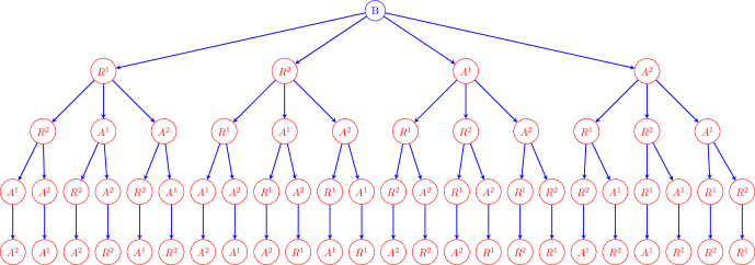
Figure 2: Possible progresses of $\left({B\texttt{ vs }((R^{1},A^{1}),(R^{2},A^{2}))}\right).$

The Blue force will focus its fire power to whichever possesses the largest threatening rate. However, let us emphasize that if $R^{1}$ or $R^{2}$ is eliminated then the Blue force doesn’t have to fight $A^{1}$ or $A^{2}$. Moreover, if both $R^{1}$ and $R^{2}$ are terminated, the combat ends promptly (since the Blue force is no longer attrited). Therefore, the combat may actually consists of two or three stages only. Actual stages are depicted in Figure 3.

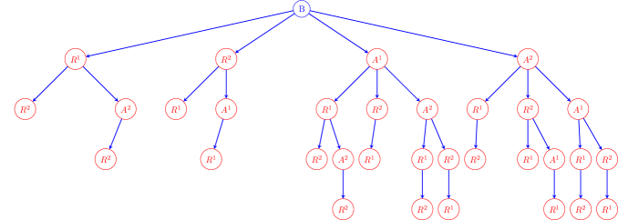
Figure 3: Actual stages of the combat $\left({B\texttt{ vs }((R^{1},A^{1}),(R^{2},A^{2}))}\right).$

Corollary 2.

For $n=1$ our model becomes $\left({B\texttt{ vs }(R^{1},A^{1})}\right).$ Then the optimal fire allocation of $B$ is :

$$P^{*}=\begin{cases}(1,0)\textrm{ if }b_{1}\geq b_{2},\\ (0,1)\textrm{ if }b_{1}\leq b_{2}.\end{cases}$$ (14)

This result has been established in the work of Kim (Kim ).

III Numerical illustrations

In this section, we will present numerical experiments for three typical cases of Corollary 1.

III.1 Experiment 1: The Armed forces are attacked first

Let us consider equation (1) with the following parameters:

$(\alpha_{d}^{1},\alpha_{c}^{1})$	$(\alpha_{d}^{2},\alpha_{c}^{2})$	$(r_{R^{1}},r_{R^{2}},r_{A^{1}},r_{A^{2}})$
$(0.4,0.8)$	$(0.5,0.7)$	$(0.4,0.35,0.3,0.4)$

Table 1: Parameters for Experiment 1.

together with the following initial conditions:

$${{B}_{0}}=350;{R}_{0}^{1}=120;\,\,R_{0}^{2}=100;\,{A}_{0}^{1}=50;\,A_{0}^{2}=60.$$

For these parameters, "threatening rates" are computed as

$${b}_{1}=0.32;\,\,{b}_{2}=0.245;\,{b}_{3}=0.288;\,{b}_{4}=0.133.$$

Applying Corollary 1, we conclude that the Blue force will focus its power to attack $R^{1}$ in the first stage. After the first stage, $R^{1}$ is eliminated and therefore $A^{1}$ is not necessarily to be attacked. For the second stage, applying Corollary 2, the Blue force will concentrate its fire power to $R^{2}$. Concluding $R^{2}$, the battle ends. To sum up, the optimal fire allocation for $B$ is

$$P^{*}=(1,0,0,0)\rightarrow(0,1,0,0).$$

We compare the optimal fire allocation with the strategy

$${{P}_{1}}=\left(0,1,0,0\right)\to\left(1,0,0,0\right).$$

The allocation of $P_{1}$ is similar to $P^{*}$ but in reverse order. Another allocation used to compare is

$$P_{2}=(0,0,1,0)\rightarrow(0,1,0,0)\rightarrow(1,0,0,0).$$

The progress of the battles with three fire allocations and number of Blue’s troops are reflected in Figure 4.

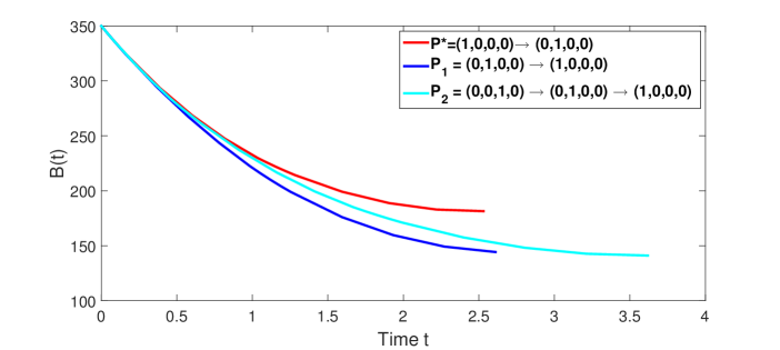
Figure 4: Number of Blue’s troops vs Time in Experiment 1.

III.2 Experiment 2: One of the supply agents is attacked first

Let us consider equation (1) with the following parameters:

$(\alpha_{d}^{1},\alpha_{c}^{1})$	$(\alpha_{d}^{2},\alpha_{c}^{2})$	$(r_{R^{1}},r_{R^{2}},r_{A^{1}},r_{A^{2}})$
$(0.4,0.8)$	$(0.3,0.7)$	$(0.4,0.5,0.3,0.4)$

Table 2: Parameters for Experiment 2.

together with the following initial conditions:

$${{B}_{0}}=350;{R}_{0}^{1}=120;\,\,R_{0}^{2}=150;\,{A}_{0}^{1}=50;\,A_{0}^{2}=40.$$

For these parameters, "threatening rates" now become

$${b}_{1}=0.32;\,\,{b}_{2}=0.35;\,{b}_{3}=0.288;\,{b}_{4}=0.6.$$

By Corollary 1, we derive that the Blue force should concentrate its power to attack $A^{2}$ in the first stage. After the first stage, $A^{2}$ is excluded, and the threatening rates must be recalculated as follows:

$$b_{1}=0.32;\,b_{2}=0.15;\,b_{3}=0.288.$$

From this observation, the strategy for the second stage is concentrating firepower to $R^{1}$. When $R^{1}$ is got rid of, $A^{1}$ doesn’t need to be eliminated and $R^{2}$ must obviously be targeted in the third stage. In conclusion, the optimal fire allocation for $B$ is

$$P^{*}=(0,0,0,1)\rightarrow(1,0,0,0)\rightarrow(0,1,0,0).$$

We now measure the differences between $P^{*}$ and two fire allocations

$${{P}_{1}}=\left(1,0,0,0\right)\to\left(0,1,0,0\right)$$

and

$${{P}_{2}}=\left(0,0,1,0\right)\to\left(1,0,0,0\right).$$

The allocation of $P_{1}$ is similar to $P^{*}$ but it does not include an offence against $A^{2}$. On the other hand, $P_{2}$ indicates that Blue force will choose to attack supply agent $A^{1}$ instead of $A^{2}$ in the first stage and then focus on $R^{1}$. The advancement of the battles depicted in Figure 5 demonstrate that the Blue force can still win with strategy $P_{1}$ but it loses with strategy $P_{2}$.

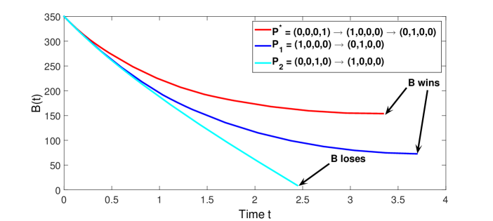
Figure 5: Number of Blue’s troops vs Time in Experiment 2.

III.3 Experiment 3: Both of the supply agents are attacked in early stages

The following parameters are now use with our model:

$(\alpha_{d}^{1},\alpha_{c}^{1})$	$(\alpha_{d}^{2},\alpha_{c}^{2})$	$(r_{R^{1}},r_{R^{2}},r_{A^{1}},r_{A^{2}})$
$(0.4,0.8)$	$(0.3,0.7)$	$(0.2,0.5,0.3,0.4)$

Table 3: Parameters for Experiment 3.

together with the following initial conditions:

$${{B}_{0}}=400;{R}_{0}^{1}=120;\,\,R_{0}^{2}=150;\,{A}_{0}^{1}=50;\,A_{0}^{2}=40.$$

Threatening rates from (2) now become

$${b}_{1}=0.16;\,\,{b}_{2}=0.35;\,{b}_{3}=0.288;\,{b}_{4}=0.6.$$

It follows that the Blue force should concentrate its power to attack $A^{2}$ in the first stage. After the first stage, $A^{2}$ is extinguished, and the recalculated threatening rates are as follows:

$$b_{1}=0.16;\,b_{2}=0.15;\,b_{3}=0.288.$$

The supply agent $A^{1}$ will therefore be targeted in the second stage. After two stages, supply agents are left out of the picture and the armed force $R^{1}$ should be targeted in the third stage since it possesses higher threatening rate. In conclusion, the optimal fire allocation for $B$ is

$$P^{*}=(0,0,0,1)\rightarrow(0,0,1,0)\rightarrow(1,0,0,0)\rightarrow(0,1,0,0).$$

In order to justify the optimality of $P^{*}$, the following fire allocations will be brought into comparison

$${{P}_{1}}=\left(0,0,1,0\right)\rightarrow\left(1,0,0,0\right)$$

and

$${{P}_{2}}=\left(0,0,0,1\right)\rightarrow(0,1,0,0)\rightarrow(0,0,1,0)\rightarrow\left(1,0,0,0\right).$$

The allocation of $P_{1}$ is opposing to $P^{*}$ as it indicates that the Blue force will target $A^{1}$ instead of $A^{2}$ in the first stage and the armed force $R^{1}$ instead of a supply agent in the second stage. Whereas, $P_{2}$ is similar to the optimal fire allocation $P^{*}$. It demonstrates that Blue force will choose to attack supply agent $A^{2}$ in the first stage, just like $P^{*}$, and then focus on $R^{2},A^{1},R^{1}$ in the later stages, respectively. The development of the battles portrayed in Figure 6 demonstrate that the Blue force can still win with strategy $P_{2}$ but it loses with strategy $P_{1}$.

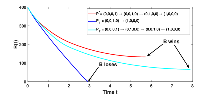
Figure 6: Number of Blue’s troops vs Time in Experiment 3.

IV Conclusion

In this work, we have introduced a novel model for battle with supplies. Computing the "threatening rates" of the Red party’s entities, we managed to show the optimal fire allocation of the Blue party. Basically, the Blue force will target entity possessing the largest "threatening rate". These results have improved and generalized some known results in this field.

References

References

• (1) F. W. Lanchester, Aircraft in Warfare: The Dawn of the Fourth Arm, (Constable, London, 1916).
• (2) S. J. Deitchman, "A Lanchester model of guerilla warfare", Operations Research, 10, 818-827 (1962).
• (3) M. B. Schaffer, "Lanchester models of guerrilla engagements", Operations Research, 16, 457-488 (1968).
• (4) T. S. Schreiber, "Letter to the editor: Note on the combat value of intelligence and command control systems", Operations Research, 12(3), 507-510 (1964).
• (5) E. H. Kaplan, A. Mintz, M. Shaul, C. Samban, "What happened to suicide bombings in Israel? Insights from a terror stock model", Studies in Conflict and Terrorism, 28, 225-235 (2005).
• (6) M. Kress, R Szechtmann "Why defeating insurgencies is hard: the effect of intelligence in counter insurgency operations - a best-case scenario", Operations Research, 57(3), 578-585 (2009).
• (7) J. G. Taylor, "Lanchester-type models of warfare and optimal control", Naval Research Logistics Quarterly, 21, 70-106 (1974).
• (8) K. Y. Lin, N. J. MacKay, "The optimal policy for the one-against-many heterogeneous Lanchester model", Operations Research Letters, 42, 473-477 (2014).
• (9) G. Feichtinger, A. Novak, S. Wrzaczek, "Optimizing counter-terroristic operations in an asymmetric Lanchester model", in: 15th IFAC Workshop on Control Applications of Optimization, 27-32 (2012).
• (10) M. D. Hy, M. A. Vu, N. H. Nguyen, A. N. Ta, D. V. Bui, "Optimization in an asymmetric Lanchester (n,1) model", The Journal of Defense Modeling and Simulation: Applications, Methodology, Technology , 17(1), 117-122 (2020).
• (11) D. S. Alberts, J. J. Garstka, F. P. Stein, NETWORK CENTRIC WAR FARE: Developing and Leveraging Information Superiority, (CCRP, 1999).
• (12) W. A. Owens, "The emerging U.S System-of-systems", in: U.S. Naval Institute Proceedings, 36-9 (May 1995).
• (13) H. D. Tunnell, "The U.S army and network-centric warfare a thematic analysis of the literature", in: MILCOM 2015 - 2015 IEEE Military Com munications Conference, 2015, 889-894.
• (14) H. D. Tunnell, "Network-centric warfare and the data-information knowledge-wisdom hierarchy", Military Review, 94(3), 43-50 (2004).
• (15) D. Kim, H. Moon, H. Shin, "Some properties of nonlinear Lanchester equations with an application in military", Journal of Statistical Computation and Simulation, 87(13), 2470-2479 (2017).