A Reduced Order Cut Finite Element method for geometrically parameterized steady and unsteady Navier–Stokes problems

Abstract.

We focus on steady and unsteady Navier–Stokes flow systems in a reduced-order modeling framework based on Proper Orthogonal Decomposition within a levelset geometry description and discretized by an unfitted mesh Finite Element Method. This work extends the approaches of [39, 41, 43] to nonlinear CutFEM discretization. We construct and investigate a unified and geometry independent reduced basis which overcomes many barriers and complications of the past, that may occur whenever geometrical morphings are taking place. By employing a geometry independent reduced basis, we are able to avoid remeshing and transformation to reference configurations, and we are able to handle complex geometries. This combination of a fixed background mesh in a fixed extended background geometry with reduced order techniques appears beneficial and advantageous in many industrial and engineering applications, which could not be resolved efficiently in the past.

1. Introduction

In the present work, we are interested in studying geometrically parameterized steady and unsteady Navier–Stokes equations in a Eulerian framework. We rely on an approach based on unfitted mesh Finite Element Method, which shows its flexibility especially when domains are subject to large deformations, and classical methods such as the Finite Element Method (FEM) fail.

In general, new computational tools have been invented and studied over the past years to solve numerically Navier-Stokes problems: the classical FEM is a powerful tool to discretize the physical domain of interest and simulate the behavior of the solution, and its efficiency has been proven in a wide range of applications [14, 49, 46]. Nonetheless, FEM capability to handle geometrically parametrized problems comes to a limit, this limit being given by extremely complex geometries, but also by situations where large deformations, fractures, contact points occur. As an alternative to classical FEM, we can consider Finite Element (FE) approximations of the physical fields that are not fitted to the actual physical geometry. The FE approximations are then cut at the boundaries and interfaces: this gives rise to the Cut Finite Element Method (CutFEM). For a more precise idea and for more rigorous definitions of what “cutting” a physical field means, and for a detailed introduction to CutFEM, we refer to [18] and references therein.
The repeated solution of parametrized problems discretized by CutFEM on the other hand, is an expensive task (whose cost essentially depends on the size of the underlying background mesh), especially in complex geometries. It is precisely at this point that the Reduced Basis Method (RBM) comes into play. It is well known that the Reduced Basis Method is an extremely powerful tool to obtain a speedup in the simulation of the behavior of the solution of the system. The method relies on a set of already computed solutions (snapshots) for different parameter values: see, for example, [33, 52, 32]. Therein, these snapshots are FE approximations of the truth solution, thus the RBM relies on the FEM. Even though in general there are several methods that can be employed to project the full order system to a reduced system, see for example [50, 25, 38, 47, 26, 27], in the present work we will employ the Proper Orthogonal Decomposition (POD). We use a fixed background geometry and mesh: this approach leads to important advantages whenever a geometry deforms,[39], and it overcomes several related limitations in efficiency, compared with traditional FEM, see e.g.[5, 42, 41]. For the reader interested in Reduced Order Methods based on classical FEM we refer to: [33] for Proper Orthogonal Decomposition, to [25, 33, 38, 47, 50] for greedy approaches and certified Reduced Basis Method, to [25, 26, 27] for Proper Generalized Decomposition (PGD), to [50, 31] for linear elliptic and parabolic systems and to [62, 30, 48] for nonlinear problems.
The aim of this work is to implement a Reduced Basis Method for the stationary and time–dependent Navier–Stokes equations, that relies on an unfitted CutFEM discretization. Already existing results on RBM applied to Navier Stokes problems with standard FEM can be found in the classical literature, see for example [35, 48, 58]; for other results concerning RBM based on embedded FEM for different kind of problems, see for example [42, 41], as well as [43] for Navier-Stokes with the Shifted Boundary Method. Nevertheless, there is still a fundamental lack in the literature for results that combine the RBM with an unfitted CutFEM discretization: indeed, a first important reference in this framework is represented by [39], where the authors focus on steady, linear model problems such as the Stokes problem and the Darcy problem. The results presented in this manuscript represent the first step in the application of unfitted CutFEM based Reduced Basis Method to time–dependent, nonlinear fluid flows: to the best of our knowledge, indeed, existing results in the reduced order model framework include only linear problems, see [39].

The paper is structured as follows: in Section 2 we introduce some basic notions of unfitted mesh Finite Element discretization, as well as some notation that will be used throughout the work. In Section 3 we introduce the steady Navier–Stokes equations with incompressibility constraint in a fluid domain where the shape of some of the boundaries is described through a levelset function depending on a geometrical parameter. In Section 3.2 we state the weak formulation of the problem of interest, which is based on Nitsche’s method with penalty term, and a Ghost Penalty stabilization. In Section 3.3 we present the Proper Orthogonal Decomposition, with a focus in Section 3.3.1 on the lifting of non–homogeneous Dirichlet boundary conditions that are imposed strongly, and with a focus in Section 3.3.2 on the natural smooth extension, a technique that is here used to obtain improved parameter–independent reduced basis functions. In Section 3.4 we present the online system to be solved, and finally in Section 3.5 we show some numerical results. In Section 4 we move then to the unsteady Navier–Stokes equations, formulated over the same physical domain as the one previously considered: the strong formulation is presented in Section 4.1. In Section 4.2 we state the weak formulation after time discretization and after spatial discretization. In Section 4.3 we present the POD technique used in the case of time–dependent parametrized problems, and in Section 4.4 we present some numerical results. In Section 5 we introduce another computational fluid dynamics test case, where an obstacle is now immersed in a fluid. In Section 5.1.2 we briefly recall the weak formulation, as well as the POD and the online system in Section 5.2; numerical results are provided in Section 5.3. Conclusions and perspectives are provided in Section 6.

2. Full order discretization by CutFEM: an introduction to terminology and definitions

The aim of this Section is to introduce some basic notions and definitions in the CutFEM framework: these definitions will be employed in the discrete formulation of the problems that we present hereafter.

As mentioned in the Introduction, unfitted Finite Element discretizations are extremely useful for the numerical simulation of problems whose physical domain undergoes a significant change in its topology: contact points occur, overlapping domains, changes in the shape due to geometrical parametrization are just some of many examples. The fundamental idea at the core of unfitted discretization is the realization of a fixed background mesh: this mesh, once generated, will not change, thus avoiding any additional expensive procedures as remeshing. The physical domain over which the problem of interest is formulated will intersect the elements of the background mesh, creating a natural subdivision into two meshes: an active mesh and an inactive mesh; in addition, the boundary of the physical domain will cut, in an arbitrary way, some of the elements of the background mesh. All these concepts are at the basis of every unfitted FEM discretization: let us now see more in detail how all these entities are defined.

Figure 1. Left: the physical domain of interest $\Omega$ (dark blue), with inflow boundary $\Gamma_{in}$, outflow boundary $\Gamma_{out}$, and top and bottom boundaries which are denoted here $\Gamma_{D}$. The boundary $\Gamma$ is the boundary delimited by the green sets, and is the immersed boundary. Right: the background mesh $\hat{\mathcal{I}}_{h}$.

Figure 2. Left: the portion of the mesh intersected by the immersed boundary $\Gamma$, namely $\mathcal{I}_{\Gamma}$, is depicted in red. Right: the fictitious domain $\Omega^{*}_{h}$ is depicted in red, and is determined by the elements $T$ of the active mesh $\mathcal{I}_{h}$.

Let $\Omega$ be the physical domain over which our problem is formulated, and let $\hat{\mathcal{I}}_{h}$ be a fixed background mesh of our choice, of mesh size $h>0$, covering $\Omega$, with inlet boundary $\Gamma_{in}=\{\bm{x}\in\Gamma:\bm{u}(\bm{x},t)\cdot\bm{n}<0\}$ (see Figure 1). Given a background mesh, this identifies in a natural way the active mesh $\mathcal{I}_{h}$, which is the portion of the background mesh made by elements $T$ that are actually intersected by the physical domain:

$$\mathcal{I}_{h}:=\{T\in\hat{\mathcal{I}}_{h}\colon\Omega\cap T\neq\emptyset\}.$$

Then, starting from the active mesh we can define a domain $\Omega_{h}^{*}$ as follows:

$$\Omega_{h}^{*}=\bigcup\limits_{T\in\mathcal{I}_{h}}T.$$

Two situations can present: $\mathcal{I}_{h}$ is a

• boundary fitted mesh if $\overline{\Omega^{*}_{h}}=\overline{\Omega}$;

• unfitted mesh if $\overline{\Omega}\subsetneq\overline{\Omega^{*}_{h}}$. In this case $\Omega^{*}_{h}$ is the so called fictitious domain, and we have an unfitted discretization of the problem of interest (see Figure 2). This is the kind of discretization that will adopted throughout the paper.

For unfitted meshes a crucial role is played by those elements $T$ of the active mesh that are cut by the immersed boundary $\Gamma$ of the physical domain $\Omega$:

$$\mathcal{I}_{\Gamma}:=\{T\in\mathcal{I}_{h}\colon T\cap\Gamma\neq\emptyset\}.$$

Related to the set $\mathcal{I}_{\Gamma}$ we can also define the set of facets that belong to elements intersected by the boundary:

$$\mathcal{F}_{\Gamma}:=\{F\in\mathcal{F}\colon F\text{ is a facet of an element }T\in\mathcal{I}_{\Gamma}\}.$$

In the framework of unfitted meshes and unfitted Finite Element discretization, the role of the cut elements $T\in\mathcal{I}_{\Gamma}$ is important: indeed, it has been shown (see for example [18, 21, 20, 16]) that stability issues may arise, depending on the quality of the cut, namely depending on how the boundary $\Gamma$ cuts an element $T$. In order to overcome the dependency of the stability and a priori estimates on the position of the interface, and the overall ill-conditioning of the global system matrix due to bad intersections, Burman et al. introduced a stabilization technique called Ghost Penalty, see [18, 21, 19, 15]. The idea of the Ghost Penalty stabilization is to adding weakly consistent operators with the aim of having a better control on the solution in $\overline{\Omega_{h}^{*}}\setminus\overline{\Omega}$. We will return more into the details of the Ghost Penalty stabilization used in Section 3.2. We remark that the Ghost Penalty technique is the stabilization that will be used throughout the paper, nevertheless there are alternative techniques like the residual-based stabilization (RBVM), see for example [56].

3. Steady Navier–Stokes

In the following, we focus on the steady incompressible Navier–Stokes equations, which are formulated within an Eulerian formalism. We first introduce the problem formulation, and then we present the discretized version of the original problem, in the CutFEM framework.

Figure 3. Instance geometry of the problem for $\theta=0.37$: the fluid domain $\Omega(\theta)$ (blue) has an inlet boundary $\Gamma_{in}$ on the left and an outlet boundary $\Gamma_{out}$ on the right. The rest of the boundaries ($\Gamma_{D}$) are Dirichlet type boundaries. The shape of $\mathcal{D}(\theta)$ (red) is described by the levelset function $\Phi_{\theta}(x,y)$ (see Equation 2). The immersed boundary $\Gamma_{\theta}$ is depicted in green.

3.1. Strong formulation

Let $\mathcal{R}$ be a background rectangular domain in $\mathbb{R}^{2}$, and let $\mathcal{D}(\theta)\subset\mathcal{R}$ be a bounded subset of $\mathcal{R}$, whose boundary is described through a levelset function $\{\Phi_{\theta}=0\}$, where $\Phi_{\theta}$ is an implicit function depending on a geometrical parameter $\theta$. The physical domain over which our problem is formulated is $\Omega(\theta):=\mathcal{R}\setminus\mathcal{D}(\theta)$, and is depicted in Figure 3 for a given value of $\theta$. In Figure 3 we can see the inlet boundary $\Gamma_{in}$, the outlet boundary $\Gamma_{out}$, as well as the top and bottom wall of the domain, which are denoted by $\Gamma_{D}$, since Dirichlet conditions will be applied there. We further denote $\Gamma_{\theta}$ the immersed boundary, that is, the remaining part of the boundary $\partial\Omega(\theta)$ that is in common to $\mathcal{D}(\theta)$. We denote by $\mathcal{P}$ the parameter space to which $\theta$ belongs. Under these assumptions, our problem of interest reads: for every $\theta\in\mathcal{P}$, find $\bm{u}(\theta)\colon\Omega(\theta)\mapsto\mathbb{R}^{2}$ and $p(\theta)\colon\Omega(\theta)\mapsto\mathbb{R}$ such that:

(1) $$\begin{cases}-\mu\Delta\bm{u}(\theta)+\nabla p(\theta)+(\bm{u}(\theta)\cdot\nabla)\bm{u}(\theta)=\bm{f}(\theta)\quad\text{in $\Omega(\theta)$},\\ \text{div}\bm{u}(\theta)=0\quad\text{in $\Omega(\theta)$},\end{cases}$$

where $\mu$ is the fluid viscosity and $\bm{f}(\theta)$ is the fluid volume external force. Problem (1) is completed by the following boundary conditions: at the inlet boundary $\Gamma_{in}$ we impose a prescribed inlet velocity (througout the manuscript we choose a parameter independent inlet profile) $\bm{u}(\theta)=\bm{u}_{in}$; we then have a zero outflow condition on $\Gamma_{out}$, a no–slip boundary condition $\bm{u}(\theta)\cdot\bm{n}_{D}=0$ on $\Gamma_{D}$, with $\bm{n}_{D}$ the outgoing normal to $\Gamma_{D}$, and a no–slip boundary condition $\bm{u}(\theta)=\bm{0}$ on $\Gamma_{\theta}$.

3.1.1. Geometrical parametrization

For the problem considered in this section the expression of the levelset function is the following:

(2) $$\Phi_{\theta}(x,y)={} -\Bigl{(}\left|A(x)+B(x)-1\right|+\left|{A(x)-B(x)-2}\right|+D(x)\Bigr{)}$$

$$\cdot\Bigl{(}\left|{A(x)+C(x)-1}\right|+\left|{A(x)-C(x)-2}\right|+D(x)\Bigr{)},$$

where $A(x)=\sqrt{k_{1}}\left|x-k_{3}\right|$, $B(x)=\sqrt{k_{2}}\left|y-k_{4}\right|$, $C(x)=\sqrt{k_{2}}\left|y-k_{5}\right|$ and $D(x)=e^{-\theta}(k_{1}(x-k_{3})^{2})\theta-4$.

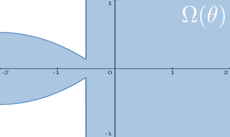
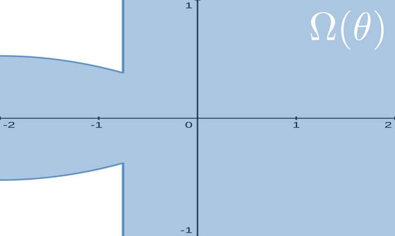
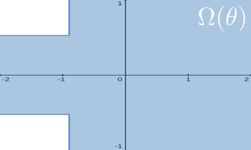
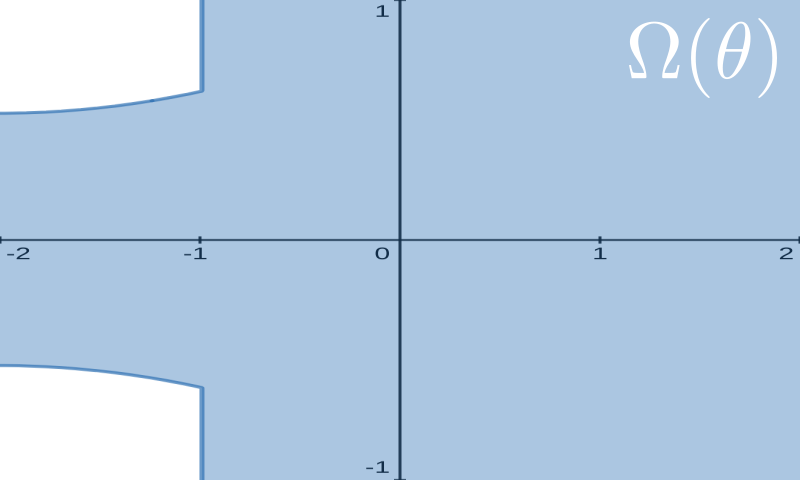
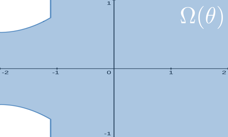
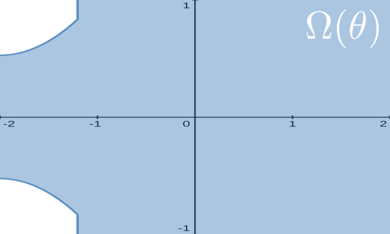
Figure 4. Six examples of solid walls, described by the levelset $\{\Phi_{\theta}=0\}$. From left to the right, the levelset for $\theta=-0.1,-0.06,0,0.18,0.37,0.50$.

The values of the constants $k_{1},k_{2},k_{3},k_{4},k_{5}$ are reported in Table 1. To have a better idea of how the shape of the walls changes by varying the parameter $\theta$, the reader is referred to Figure 4.

Table 1. Values for the constants in the levelset equation (2).

Constant	Value
$k_{1}$	$10$
$k_{2}$	$10$
$k_{3}$	$-2$
$k_{4}$	$-1$
$k_{5}$	$1$

3.2. Discrete weak formulation

As we can see from Figure 3, the background mesh $\hat{\mathcal{I}}_{h}$ is a rectangular mesh made by triangular elements. By choosing an unfitted mesh, once we have defined a background mesh, there is no need to remesh every time the parameter $\theta$ changes (and hence every time the shape of the levelset in dark grey in Figure 3 changes). Before going any further, we remark that we decide to impose the Dirichlet boundary conditions in the following way: the no–slip condition on the immersed boundary $\Gamma_{\theta}$ is imposed weakly, whereas the inflow condition, as well as the homogeneous Dirichlet condition on $\Gamma_{D}$ are imposed strongly. Let us now introduce the following discrete approximation spaces:

$$\begin{split}V_{h,{{2}}}(\theta)&:=\{\bm{v}_{h}\in C_{0}(\Omega^{*}_{h}(\theta))^{2}\colon\bm{v}_{h}|_{T}\in(\mathcal{P}^{{2}}(T))^{2},\quad\forall T\in\mathcal{I}_{h}(\theta)\},\\ Q_{h,1}(\theta)&:=\{q_{h}\in C_{0}(\Omega^{*}_{h}(\theta))\colon q_{h}|_{T}\in\mathcal{P}^{1}(T),\quad\forall T\in\mathcal{I}_{h}(\theta)\},\end{split}$$

where $\mathcal{I}_{h}(\theta)$ and $\Omega_{h}^{*}(\theta)$ are respectively the active mesh and the fictitious domain corresponding to the physical domain $\Omega(\theta)$, as defined in Section $2.1$: these spaces clearly depend on $\theta$, since the levelset geometry changes according to the parameter. We then define:

$$\begin{split}V_{h,{{2}}}^{D}\theta)&:=\{\bm{v}_{h}\in V_{h,{{2}}}(\theta)\colon\bm{v}_{h}=\bm{u}_{in}\text{ on }\Gamma_{in}\text{ and }\bm{v}_{h}\cdot\bm{n}_{D}=0\text{ on }\Gamma_{D}\},\\ V_{h,{{2}}}^{0}(\theta)&:=\{\bm{v}_{h}\in V_{h,{{2}}}(\theta)\colon\bm{v}_{h}=\bm{0}\text{ on }\Gamma_{in}\}\end{split}$$

The discretized weak formulation of the problem, with Nitsche’s Method and Ghost Penalty terms then reads: find $(\bm{u}_{h}(\theta),p_{h}(\theta))\in V_{h,2}^{D}(\theta)\times Q_{h,1}(\theta)$ such that for all test functions $(\bm{v}_{h}(\theta),q_{h}(\theta))\in V_{h,2}^{0}(\theta)\times Q_{h,1}(\theta)$:

(3) $$\mathcal{A}({\bm{u_{h}}}(\theta),p_{h}({\theta});\bm{v}_{h}(\theta),q_{h}(\theta))=\mathcal{L}(\bm{v}_{h}(\theta)),$$

where:

$$\mathcal{A}(\bm{u}_{h}(\theta),p_{h}(\theta);\bm{v}_{h}(\theta),q_{h}(\theta)) = {a_{h}(\bm{u}_{h}(\theta),\bm{v}_{h}(\theta))+b_{h}(p_{h}(\theta),\bm{v}_{h}(\theta))-b_{h}(q_{h}(\theta),\bm{u}_{h}(\theta))+}$$

$${+c_{h}(\bm{u}_{h}(\theta);\bm{u}_{h}(\theta),\bm{v}_{h}(\theta)+g^{GP}(\bm{u}_{h}(\theta),\bm{v}_{h}(\theta);p_{h}(\theta),q_{h}(\theta))}$$

$$\mathcal{L}(\textbf{v}_{h}) = (f,v_{h})_{\Omega(\theta)}$$

In the previous equation we have the following bilinear (and trilinear) forms:

$$a_{h}(\bm{u}_{h}(\theta),\bm{v}_{h}(\theta)) = {\mu(\nabla\bm{u}_{h}(\theta),\nabla\bm{v}_{h}(\theta))_{\Omega(\theta)}-\mu(\nabla\bm{u}_{h}(\theta)\bm{n}_{\Gamma},\bm{v}_{h}(\theta))_{\Gamma_{\theta}}-}$$

$${-\mu(\bm{u}_{h}(\theta),\nabla\bm{v}_{h}(\theta)\bm{n}_{\Gamma})_{\Gamma_{\theta}}+{\gamma\mu/}{h}(\bm{u}_{h}(\theta),\bm{v}_{h}(\theta))_{\Gamma_{\theta}}}$$

$${{+{\gamma\phi}/{h}(\bm{u_{h}}(\theta)\cdot\bm{n}_{\Gamma},\bm{v_{h}}(\theta)\cdot\bm{n}_{\Gamma})_{\Gamma_{\theta}}}}$$

$$c_{h}(\bm{u}_{h}(\theta);\bm{u}_{h}(\theta),\bm{v}_{h}(\theta)) = {((\bm{u}_{h}(\theta)\cdot\nabla)\bm{u}_{h}(\theta),\bm{v}_{h}(\theta))_{\Omega(\theta)}}-{((\bm{u}_{h}(\theta)\cdot\bm{n})\bm{u}_{in},\bm{v}_{h}(\theta))_{\Gamma_{in}}}$$

$$b_{h}(p_{h}(\theta),\bm{v}_{h}(\theta)) = -{(p_{h}(\theta),\nabla\cdot\bm{v}_{h}(\theta))_{\Omega(\theta)}+(p_{h}(\theta)\bm{n}_{\Gamma},\bm{v}_{h}(\theta))_{\Gamma_{\theta}}}$$

$$g^{GP}(\bm{u}_{h}(\theta),\bm{v}_{h}(\theta);p_{h}(\theta),q_{h}(\theta)) = {g_{u}^{GP}(\bm{u}_{h}(\theta);\bm{u}_{h}(\theta),\bm{v}_{h}(\theta))+g^{GP}_{p}(\bm{u}_{h}(\theta);p_{h}(\theta),q_{h}(\theta))}$$

$${{+g_{\mu}^{GP}(\bm{u}_{h}(\theta),\bm{v}_{h}(\theta))+g_{\beta}^{GP}(\bm{u}_{h}(\theta);\bm{u}_{h}(\theta),\bm{v}_{h}(\theta))}}$$

s where $\bm{n}_{\Gamma}$ is the outward pointing normal to the immersed boundary $\Gamma_{\theta}$, and $h$ is the mesh size. The term $-((\bm{u}_{h}(\theta)\cdot\bm{n})\bm{u}_{h}(\theta),\bm{v}_{h}(\theta))_{\Gamma_{in}}$ in the trilinear form $c_{h}$, where $\bm{n}$ in this term is the outgoing normal to the inlet boundary, that accounts for the inlet flow $\Gamma_{in}=\{\bm{x}\in\Gamma:\bm{u}(\bm{x},t)\cdot\bm{n}<0\}$ (see for example [10]). The ghost penalties $g_{u}^{GP}(\bm{u}_{h}(\theta),\bm{v}_{h}(\theta))$, $g^{GP}_{p}(p_{h}(\theta),q_{h}(\theta))$, $g_{\mu}^{GP}(\bm{u}_{h}(\theta),\bm{v}_{h}(\theta))$, and $g^{GP}_{\beta}(p_{h}(\theta),q_{h}(\theta))$ are defined as:

$$g_{u}^{GP}(\bm{u}_{h}(\theta);\bm{u}_{h}(\theta),\bm{v}_{h}(\theta)) = {{{\gamma_{u}\sum_{F\in\mathcal{F}_{{\Gamma}_{\theta}}}\phi_{u,F,\theta}h^{2j+1}(\mathopen{[\![}\nabla\cdot\partial_{n}^{j}\bm{u}_{h}(\theta)\mathclose{]\!]},\mathopen{[\![}\nabla\cdot\partial_{n}^{j}\bm{v}_{h}(\theta)\mathclose{]\!]})_{F}}}},$$

$$g^{GP}_{p}(\bm{u}_{h}(\theta);p_{h}(\theta),q_{h}(\theta)) = \gamma_{p}\sum_{F\in\mathcal{F}_{\Gamma_{\theta}}}{h^{3}}{\mu}^{-1}({1}/{\text{max}({h}/{\mu}\lvert\lvert{\bm{u}}(\theta)\rvert\rvert_{\infty,T},1))}(\mathopen{[\![}\partial_{n}p_{h}(\theta)\mathclose{]\!]},\mathopen{[\![}\partial_{n}q_{h}(\theta)\mathclose{]\!]})_{F},$$

$${{g_{\mu}^{GP}(\bm{u}_{h}(\theta),\bm{v}_{h}(\theta))}} = {{{\gamma_{\mu}\sum_{j=1}^{2}\sum_{F\in\mathcal{F}_{{\Gamma}_{\theta}}}\mu h^{2j-1}(\mathopen{[\![}\partial_{n}^{j}\bm{u}_{h}(\theta)\mathclose{]\!]},\mathopen{[\![}\partial_{n}^{j}\bm{v}_{h}(\theta)\mathclose{]\!]})_{F}}}},$$

$${{g_{\beta}^{GP}(\bm{u}_{h}(\theta);\bm{u}_{h}(\theta),\bm{v}_{h}(\theta))}} = {{{\gamma_{\beta}\sum_{j=1}^{2}\sum_{F\in\mathcal{F}_{{\Gamma}_{\theta}}}\phi_{\beta,F,\theta}u_{\infty,F,\theta}^{2}h^{2j-1}(\mathopen{[\![}(\bm{u}_{h}(\theta)\cdot\nabla)\partial_{n}^{j}\bm{u}_{h}(\theta)\mathclose{]\!]},\mathopen{[\![}(\bm{u}_{h}(\theta)\cdot\nabla)\partial_{n}^{j}\bm{v}_{h}(\theta)\mathclose{]\!]})_{F}}}}.$$

In the previous equations, $\mu$ is the fluid kinematic viscosity, $\partial_{n}$ denotes the partial derivative with respect to the normal outgoing the face $F$. We have used the following notation:

(4) $$u_{\infty,F,\theta}:={\lvert\lvert\bm{u}_{h}(\theta)\rvert\rvert_{0,\infty,F}},\quad\phi_{T,\theta}:={\mu+c_{u}\lvert\lvert\bm{u}_{h}(\theta)\rvert\rvert_{0,\infty,T}h_{T}}$$

(5) $$\phi_{\beta,T,\theta}:={\phi_{p,T,\theta}=h_{T}^{2}\phi_{T,\theta}^{-1}},\quad\phi_{u,T,\theta}:={\phi_{T,\theta}},$$

where $h_{T}$ is the characteristic element length. Then, $\phi_{\beta,F,\theta}$, $\phi_{u,F,\theta}$ and $\phi_{p,F,\theta}$ are the corresponding face averages. In order to simplify the implementation and the exposition, we choose here $c_{u}=1.0$. The terms appearing in the bilinear form $a_{h}(\bm{u}_{h},\bm{v}_{h})$, in the bilinear form $b_{h}(p_{h}(\theta),\bm{v}_{h}(\theta))$ and in the trilinear form $c_{h}(\bm{u}_{h}(\theta;\bm{u}_{h}(\theta),\bm{v}_{h}(\theta))$ come from standard integration by parts of the steady Navier–Stokes equations, due to the fact that the test functions are non–vanishing on the boundary $\Gamma_{\theta}$. We then have the Nitsche terms, that have been used to weakly impose the non–slip boundary condition on $\Gamma_{\theta}$. The term $g_{\beta}^{GP}$ is a convective stabilization term which for low Reynolds number is taken $\gamma_{\beta}=0$, whereas $g_{u}^{GP}$ is the incompressibility stabilization while $g_{p}^{GP}$, $g_{\mu}^{GP}$ contain additional terms that extend the solution to the extended domain, [56, 21, 39]. We point out that we choose a symmetric Nitsche method because, even if the non–symmetric alternative leads to better stability behaviour, it can also lead to suboptimal convergence or larger $L^{2}$ errors: for more details we refer to the discussions in [17, 55]. For sake of completeness we report that the choice of a symmetric Nitsche method leads to some lack of coercivity in the bilinear form $a_{h}$, and therefore a stabilization term is consistently added. Additionally, the need for the Ghost Penalty stabilization terms is given by the fact that we are implementing an unfitted mesh discretization of the problem. With unfitted meshes indeed, it may happen that the cut elements (namely the elements $T\in\mathcal{I}_{\Gamma_{\theta}}$) are cut in an arbitrary way by the boundary $\Gamma_{\theta}$. The abritrariness of the cut position can lead to stability issues that ghost penalty stabilization terms can handle. In this manuscript we adopted the stabilization presented, for example, in [56], as well as for an analysis on the stability properties of the chosen weak formulation. The values of the constants appearing in the previous equations as well as for the supremizer enrichment are reported in Table 2.

Table 2. Constants values for the weak formulation of the problem

Constant	Value	Constant	Value
$\mu$	$0.05$	$h$	$0.07$
$\gamma$	$10$	$\gamma_{u}$	$0.001$
$\alpha$	$0.1$	$\gamma_{\mu}$	$0.1$
$\gamma_{p}$	$0.1$	$\gamma^{0}_{s}$	$0.1$
$\lambda_{s}$	$10$	$\gamma^{1}_{s}$	$0.01$

3.3. Proper Orthogonal Decomposition-Galerkin Model Reduction

We now present the Proper Orthogonal Decomposition (POD), a method that is applied to parameter-dependent problems in order to extract and create a set of reduced basis functions, with which we will subsequently perform the model order reduction. The POD method consists of two phases: one offline and one online. During the offline phase, we compute the solution of the problem of interest, for different values of the parameter $\theta$. These values of the parameter are collected from a training set $\mathcal{P}_{train}$, and the corresponding solutions are stored into a matrix, the so-called snapshots matrix. This matrix is then processed in order to extract the reduced basis functions. Afterwards, in the online phase, we employ these basis functions in a way that reduces the dimension of the original problem, and in a way that is computationally efficient for (in our case) geometrically parametrized systems. We remind hereafter that for POD-Galerkin ROMs for incompressible Navier–Stokes equations, instabilities in the approximation of the pressure may occur. We refer to [23, 29, 51] for a more detailed analysis of the problem, while for such instabilities on transient problems we refer to [37, 4, 13, 57, 28]. For SUPG and PSPG kind of stabilization we refer to [6, 53, 60, 59]. Levelset techniques with cut Finite Element Nitsche method will be employed for the parametrization and ROM focusing on a fixed, geometrical parameter independent, background mesh following approaches as in [39, 41, 42].

3.3.1. The lifting function

In view of the online phase of the reduction procedure, we have to take care of the non–homogeneous Dirichlet boundary condition at the inlet boundary $\Gamma_{in}$. We will now briefly explain how we overcome this difficulty, with the understanding that the following procedure will be carried out for all the test cases considered, even if we will not explicitly mention it again, for the sake of the simplicity of the notation.
The idea is that, in order to take care of a non–homogeneous Dirichlet boundary condition, we can define, for each parameter $\theta\in\mathcal{P}$, a lifting function $\bm{\ell}(\theta)\colon\Omega(\theta)\mapsto\mathbb{R}^{2}$, sucht that $\bm{\ell}(\theta)=\bm{u}_{in}$ on the inlet boundary $\Gamma_{in}$ and $\bm{\ell}(\theta)\cdot\bm{n}_{D}=0$ on $\Gamma_{D}$. Once we have done this, we can define a homogenized velocity

$$\bm{u}^{0}(\theta):=\bm{u}(\theta)-\bm{\ell}(\theta),$$

with $\bm{u}^{0}(\theta)\in{V}_{h,2}^{0}(\theta)$. This will become important in the next paragraph, when we state the algebraic formulation of the system that we are going to solve during the online phase of the method. The reader interested in more details on the lifting function and its use is referred, for example, to [36, 6].

3.3.2. The natural smooth extension

Let us now make an important remark about the discrete function spaces and about the CutFEM solutions: as we can see from the definitions in Section 3.2, the FE velocity $\bm{u}_{h}(\theta)$ belongs to a space that is $\theta$–dependent, namely $V_{h,2}(\theta)$, and the same goes for the FE pressure $p_{h}(\theta)\in Q_{h,1}(\theta)$. This $\theta$–dependence can create numerous problems: in general we can expect that, for two different values $\theta^{1}$ and $\theta^{2}$ of the parameter, $\Omega(\theta^{1})\neq\Omega(\theta^{2})$, and therefore $\bm{u}_{h}(\theta^{1})\notin V_{h,2}(\theta^{2})$, and similarly for the pressure. This can lead to many difficulties, especially in view of the reduction procedure: in order to perform a Proper Orthogonal Decomposition we will have to compute scalar products between functions that, in theory, can belong to different discrete spaces. In order to overcome this problem, the main idea is to extend the CutFEM solutions, namely the snapshots, to the whole background mesh: this is achieved thanks to a natural smooth extension of both velocity and pressure. The realization, at the discrete level, of the natural smooth extension is carried out through the stabilization Ghost Penalty terms that appear in the weak formulation of the original problem: we refer the reader interested in more details and in the stability analysis of this procedure to [11, 45]. As we know, the CutFEM solution is defined up to $\Omega_{h}^{*}(\theta)$: as an effect of the ghost penalty stabilization, the solution smoothly goes to zero in the cut zone $\mathcal{I}_{\Gamma_{\theta}}$. Thanks to the ghost penalty stabilization then, we can simply extend the CutFEM solution to be zero in $\mathcal{R}\setminus\Omega_{h}^{*}(\theta)$, thus obtaining a solution that is defined on the whole background mesh. Another possibility, which we do not take into consideration in this manuscript, is to implement instead an harmonic extension of the CutFEM solution: we refer the reader interested in a detailed discussion on techniques to extend the snapshots to the background mesh to [39, 8]: the reason we do not pursue this idea here is that the implementation of an harmonic extension would require an additional problem to be solved for every snapshot computed, thus incrementing the cost of the reduction procedure.
We remark that the natural smooth extension is employed also in order to extend the lifting function $\ell(\theta)$ to a function that is defined on the whole background mesh. Thanks to the extension procedure we obtain snapshots $(\hat{\bm{u}}^{0}_{h}(\theta),\hat{p}_{h}(\theta))$ that are defined on the common background mesh $\hat{\mathcal{I}_{h}}$, where now $\hat{\bm{u}}^{0}_{h}(\theta):=\hat{\bm{u}}_{h}(\theta)-\hat{\ell}(\theta)$. Such extension defines a pair of velocity–pressure snapshots $(\hat{\bm{u}}^{0}_{h}(\theta),\hat{p}_{h}(\theta))$ belonging to $\theta$–independent discrete spaces:

$$\begin{split}\hat{V}_{h,2}^{0}&:=\{\hat{\bm{v}}_{h}\in C_{0}(\mathcal{R})^{2}\colon\hat{\bm{v}}_{h}|_{T}\in(\mathcal{P}^{2}(T))^{2}\text{ }\forall T\in\hat{\mathcal{I}}_{h}\text{ and }\bm{v}_{h}=\bm{0}\text{ on }\Gamma_{in}\text{ and }\bm{v}_{h}\cdot\bm{n}_{D}=0\text{ on }\Gamma_{D}\},\\ \hat{Q}_{h,1}&:=\{\hat{q}_{h}\in C_{0}(\mathcal{R})\colon\hat{q}_{h}|_{T}\in\mathcal{P}^{1}(T)\text{ }\forall T\in\hat{\mathcal{I}}_{h}\}.\end{split}$$

At this point we can define a bijection between $\hat{V}_{h,2}^{0}$ and $\mathbb{R}^{\hat{N}_{u}^{h}}$ (respectively $\hat{Q}_{h,1}$ and $\mathbb{R}^{\hat{N}_{p}^{h}}$), where $\hat{N}_{u}^{h}$ and $\hat{N}_{p}^{h}$ are the dimensions of the discrete spaces $\hat{V}_{h,2}^{0}$ and $\hat{{Q}}_{h,1}$:

(6) $$\begin{cases}\underline{\textbf{u}}^{0}_{h}(\theta)=({u}_{h}^{1}(\theta),\dots,u_{h}^{\hat{N}_{u}^{h}}(\theta))^{T}\in\mathbb{R}^{\hat{N}_{u}^{h}}\iff\hat{\bm{u}}^{0}_{h}(\theta)=\sum_{i=1}^{\hat{N}_{u}^{h}}u_{h}^{i}(\theta)\hat{\bm{\varphi}}^{i}\in\hat{V}_{h,2}^{0},\\ \underline{p}_{h}(\theta)=({p}_{h}^{1}(\theta),\dots,p_{h}^{\hat{N}_{p}^{h}}(\theta))^{T}\in\mathbb{R}^{\hat{N}_{p}^{h}}\iff p_{h}(\theta)=\sum_{i=1}^{\hat{N}_{p}^{h}}{p}_{h}^{i}(\theta)\hat{\zeta}^{i}\in\hat{{Q}}_{h,1},\\ \end{cases}$$

where $\hat{\bm{\varphi}}^{i}$ and $\hat{\zeta^{i}}$ are the parameter–independent basis functions of the FE spaces $\hat{V}_{h,2}^{0}$ and $\hat{Q}_{h,1}$ respectively. We can now introduce the following forms:

$$\hat{a}_{h}(\hat{\bm{\varphi}}^{i},\hat{\bm{\varphi}}^{q};\theta) := {\mu(\nabla\hat{\bm{\varphi}}^{i},\nabla\hat{\bm{\varphi}}^{q})_{\mathcal{R}}-\mu(\nabla\hat{\bm{\varphi}}^{i}\bm{n}_{\Gamma},\hat{\bm{\varphi}}^{q})_{\Gamma_{\theta}}}$$

$${-\mu(\hat{\bm{\varphi}}^{i},\nabla\hat{\bm{\varphi}}^{j}\bm{n}_{\Gamma})_{\Gamma_{\theta}}+{\gamma\mu}/{h}(\hat{\bm{\varphi}}^{i},\hat{\bm{\varphi}}^{q})_{\Gamma_{\theta}}}$$

$$+{\gamma\phi}/{h}(\hat{\bm{\varphi}}^{i}\cdot\bm{n}_{\Gamma},\hat{\bm{\varphi}}^{q}\cdot\bm{n}_{\Gamma})_{\Gamma_{\theta}}$$

$$\hat{c}_{h}(\hat{\bm{\varphi}}^{k};\hat{\bm{\varphi}}^{i},\hat{\bm{\varphi}}^{q};\theta) := {((\hat{\bm{\varphi}}^{k}\cdot\nabla)\hat{\bm{\varphi}}^{i},\hat{\bm{\varphi}}^{q})_{\mathcal{R}}}$$

$$\hat{b}_{h}(\hat{\zeta}^{i},\hat{\bm{\varphi}}^{q};\theta) := -{(\hat{\zeta}^{i},\nabla\cdot\hat{\bm{\varphi}}^{q})_{\mathcal{R}}+(\hat{\zeta}^{i}\bm{n}_{T},\hat{\bm{\varphi}}^{q})_{\Gamma_{\theta}}}$$

We can therefore define the following matrices:

$${\hat{\bm{A}}(\theta)_{iq}} := {\hat{a}_{h}(\hat{\bm{\varphi}}^{i},\hat{\bm{\varphi}}^{q})+\hat{c}_{h}(\hat{\bm{\ell}}(\theta);\hat{\bm{\varphi}}^{i},\hat{\bm{\varphi}}^{q})}$$

$${+\hat{c}_{h}(\hat{\bm{\varphi}}^{i};\hat{\bm{\ell}}(\theta),\hat{\bm{\varphi}}^{q})+{{{g}^{GP}_{\mu}(\hat{\bm{\varphi}}^{i},\hat{\bm{\varphi}}^{q})}}}$$

$${\hat{\bm{N}}(\underline{\textbf{u}}_{h}(\theta);\theta)_{iq}} := {\sum_{k=1}^{N_{u}^{h}(\theta)}{u}_{h}^{k}(\theta)\hat{c}_{h}(\hat{\bm{\varphi}}^{k};\hat{\bm{\varphi}}^{i},\hat{\bm{\varphi}}^{q})+}$$

$$+{{{{g}}_{u}^{GP}(\sum_{k=1}^{N_{u}^{h}}{u}_{h}^{k}(\theta)\hat{\bm{\varphi}}^{k};\hat{\bm{\varphi}}^{i},\hat{\bm{\varphi}}^{q})}+{{g}}_{\beta}^{GP}(\sum_{k=1}^{N_{u}^{h}(\theta)}{u}_{h}^{k}(\theta)\hat{\bm{\varphi}}^{k};\hat{\bm{\varphi}}^{i},\hat{\bm{\varphi}}^{q})}$$

$${\hat{\bm{B}}(\theta)_{iq}} := {\hat{b}_{h}(\hat{\zeta}^{i},\hat{\bm{\varphi}}^{q}),}$$

$${\hat{\bm{C}}(\theta)_{iq}} := {{g}^{GP}_{p}(\sum_{k=1}^{N_{u}^{h}(\theta)}{u}_{h}^{k}(\theta)\hat{\bm{\varphi}}^{k};\hat{\zeta}^{i},\hat{\zeta}^{q})}$$

Thanks to the matrices introduced, we can now state the algebraic formulation of the Navier–Stokes problem, after the snapshots extension and after the lifting of the inlet condition:

$$R({U}_{h}(\theta),\theta):=\begin{bmatrix}{\hat{\bm{A}}}(\theta)+{{\hat{\bm{N}}}}({{\underline{\textbf{u}}}^{0}_{h}}(\theta);\theta)&{\hat{\bm{B^{T}}}}(\theta)\\ {\hat{\bm{B}}}(\theta)&\hat{\bm{C}}(\theta)\end{bmatrix}\begin{bmatrix}{{\underline{\textbf{u}}}^{0}_{h}}(\theta)\\ {\underline{p}}_{h}(\theta)\end{bmatrix}-\begin{bmatrix}{{{\hat{\bm{F}}}}_{1}}(\theta)\\ {{{\hat{\bm{F}}}_{2}}}(\theta)\end{bmatrix}{{=\begin{bmatrix}0\\ 0\end{bmatrix}}},$$

where ${U}_{h}(\theta)=({\underline{\textbf{u}}}^{0}_{h}(\theta),{\underline{p}}_{h}(\theta))$, ${(\hat{\bm{F}}_{1}(\theta))_{i}}:=\int_{\mathcal{R}}\hat{\bm{\varphi}}^{i}\cdot\bm{f}\,dx+\hat{a}_{h}(\hat{\bm{\varphi}}^{i},\hat{\bm{\ell}}(\theta);\theta)+\hat{c}_{h}(\hat{\bm{\ell}}(\theta);\hat{\bm{\ell}}(\theta),\hat{\bm{\varphi}}^{i})$ and ${\hat{\bm{F}}_{2}(\theta)}=\bm{0}$ since the embedded Dirichlet boundary data $g_{D}=0$.

3.3.3. Reduced Basis generation

Let us now denote by $\theta^{(j)}$ each parameter in a finite dimensional training set $\mathcal{P}_{train}=\{\theta^{1},\dots,\theta^{M}\}$ for a large number $M$. The snapshots matrices $\bm{\mathcal{S}_{u}}$ and $\bm{\mathcal{S}_{p}}$ for the fluid velocity and the fluid pressure are defined as follows:

(7) $$\bm{\mathcal{S}_{u}}=[\hat{\bm{u}}^{0}_{h}(\theta^{1}),\dots,\hat{\bm{u}}^{0}_{h}(\theta^{M})]\in\mathbb{R}^{N_{u}^{h}\times M},\quad\bm{\mathcal{S}_{p}}=[\hat{{p}}_{h}(\theta^{1}),\dots,\hat{{p}}_{h}(\theta^{M})]\in\mathbb{R}^{N_{p}^{h}\times M}.$$

In order to make the pressure approximation stable at the reduced order level we also introduce a velocity supremizer variable $\bm{s_{h}}$: see [6, 51, 53] for a more detailed introduction to the supremizer enrichment for Navier–Stokes equation. We start with a Laplace problem for the supremizer $\bm{s}(\theta)$, $\forall\theta\in\mathcal{P}$:

(8) $$\begin{cases}-\Delta\bm{s}(\theta)=-\nabla p_{h}(\theta)\text{ in }\Omega(\theta),\\ \bm{s}(\theta)=0\text{ in }\Gamma_{in\cup D\cup out},\\ \bm{s}(\theta)=0\text{ in }\Gamma_{\theta}\end{cases}$$

Again, we impose boundary conditions (8)₂ strongly, and (8)₃ weakly, thanks to the Nitsche method. We have therefore the following discretized problem: find $\bm{s}_{h}(\theta)\in V_{h,k}^{0}(\theta)$ such that $\forall\bm{v}_{h}(\theta)\in V_{h,k}^{0}(\theta)$:

$$(\nabla\bm{s_{h}}(\theta),\nabla\bm{v_{h}}(\theta))_{\Omega(\theta)}-(\nabla\bm{s_{h}}(\theta)\bm{n}_{\Gamma},\bm{v_{h}}(\theta))_{\Gamma_{\theta}}-(\nabla\bm{v_{h}}(\theta)\bm{n}_{\Gamma},\bm{s_{h}}(\theta))_{\Gamma_{\theta}}+\frac{\lambda_{s}}{h}(s_{h}(\theta),v_{h}(\theta))_{\Gamma_{\theta}}$$

$$+\mathit{g}^{GP}(\bm{s_{h}}(\theta),\bm{v_{h}}(\theta))=-(\nabla p_{h}(\theta),\bm{v}_{h}(\theta))_{\Gamma_{\theta}},$$

where the Ghost Penalty term is given by:

$$\mathit{g}^{GP}(\bm{s_{h}}(\theta),\bm{v_{h}}(\theta))=\sum_{1\leq j\leq 2}\sum_{F\in\mathcal{F}_{\Gamma_{\theta}}}\gamma_{s}^{j}h^{2j+1}(\mathopen{[\![}\partial_{n}^{j}\bm{s_{h}}(\theta)\mathclose{]\!]},\mathopen{[\![}\partial_{n}^{j}\bm{v_{h}}(\theta)\mathclose{]\!]})_{F},$$

We employ the same natural smooth extension (and the same extended FE space used for velocity) also for the supremizer, thus obtaining the extendend snapshots $\hat{\bm{s}}_{h}$. These snapshots are then collected in the snapshot matrix

$${\bm{\mathcal{S}}_{s}}=[\hat{\bm{s}}_{h}(\theta^{1}),\dots,\hat{{\bm{s}}}_{h}(\theta^{M})]\in\mathbb{R}^{N_{u}^{h}\times M},$$

We then carry out a compression by POD on the snapshots matrices, namely $\bm{\mathcal{S}}_{u}$, $\bm{\mathcal{S}}_{s}$ and $\bm{\mathcal{S}}_{p}$, following e.g. [44]. This derives an eigenvalue problem, that for the velocity for example reads:

$${\bm{\mathcal{C}}^{u}}\bm{Q}^{u}=\bm{Q}^{u}\bm{\Lambda}^{u},\quad\mbox{\hskip 14.22636pt for }{\bm{\mathcal{C}}}^{u}_{ij}=({\hat{\bm{u}}_{h}(\theta^{i}),\hat{\bm{u}}_{h}(\theta^{j})})_{L^{2}{(\hat{\mathcal{I}}_{h})}}\mbox{,\, }i,j=1,\dots,M,$$

where $\bm{\mathcal{C}^{u}}$ is the correlation matrix derived from the $\theta$-independent snapshots, $\bm{Q}^{u}$ is an eigenvectors square matrix and $\bm{\Lambda}^{u}$ is a diagonal matrix of eigenvalues. Similar eigenvalue problems can be derived for the supremizer and for the pressure. We refer the reader interested in the details about the POD and its implementation to [34, 6]. The $i$–th reduced basis function $\bm{\Phi}_{i}^{u}$ for the fluid velocity, for example, is then obtained (possibly after $L^{2}$ normalization) by applying the snapshots matrix $\bm{\mathcal{S}}_{u}$ to the $i$–th column of the matrix $\bm{Q}^{u}$.

3.4. Online algebraic system

Thanks to the POD on the velocity snapshots and thanks to the enrichment with supremizer snapshots we obtain a set $\{\bm{\Phi}_{1}^{u},\dots,\bm{\Phi}_{N}^{u},\bm{\Phi}_{1}^{s},\dots,\bm{\Phi}_{N}^{s}\}$ of $2N$ basis functions for the reduced order approximation of the velocity, and a set $\{\Phi_{1}^{p},\dots,\Phi_{N}^{p}\}$ of $N$ basis functions for the reduced order approximation of the pressure. We define: $\hat{V}_{N}$, the enriched reduced basis space for the velocity, and $\hat{Q}_{N}$, the reduced basis space for the pressure:

$$\hat{V}_{N}=\text{span}\{\bm{\Phi}_{1}^{u,s},\ldots,\bm{\Phi}_{2N}^{u,s}\},\qquad\hat{Q}_{N}=\text{span}\{\Phi_{1}^{p},\ldots,\Phi_{N}^{p}\}$$

where $N<M$ is chosen according to the eigenvalue decay of $\bm{\Lambda}_{ii}^{u}$ and $\bm{\Lambda}_{ii}^{p}$, see for instance [50, 12]. In the definition of the reduced space for the fluid velocity, we used a unified notation: $\bm{\Phi}_{i}^{u,s}=\bm{\Phi}_{i}^{u}$ for $i=1,\dots,N$ and $\bm{\Phi}_{i}^{u,s}=\bm{\Phi}_{i}^{s}$ for $i=N+1,\dots,2N$. We also remark the fact that the finite dimensional reduced spaces $\hat{V}_{N}$ and $\hat{Q}_{N}$ are parameter–independent, thanks to the natural smooth extension performed on the snapshots. We can now introduce the online velocity $\bm{u}_{N}(\theta)$ and the online pressure $p_{N}(\theta)$:

(9) $$\bm{u}_{N}(\theta):=\sum_{i=1}^{2N}\underline{\textbf{u}}_{N}^{i}(\theta)\bm{\Phi}_{i}^{u,s}=\bm{L}_{u,s}\underline{\textbf{u}}_{N}(\theta),$$

(10) $$p_{N}(\theta):=\sum_{i=1}^{N}\underline{p}^{i}_{N}(\theta)\Phi_{i}^{p}=\bm{L}_{p}\underline{p}_{N}(\theta),$$

where $\bm{L}_{u,s}\in\mathbb{R}^{N_{u}^{h}\times 2N}$ and $\bm{L}_{p}\in\mathbb{R}^{N_{p}^{h}\times N}$ are rectangular matrices containing the FE degrees of freedom of the basis of $\hat{V}_{N}$ and $\hat{Q}_{N}$. The parameter dependent solution vector $\underline{\textbf{u}}_{N}(\theta)\in\mathbb{R}^{2N}$ and $\underline{p}_{N}(\theta)\in\mathbb{R}^{N}$ and the parameter independent reduced basis functions $\bm{\Phi}_{i}^{u,s}$, $\Phi_{i}^{p}$ are the key ingredients necessary to perform a Galerkin projection of the full system onto the aforementioned reduced basis space. By introducing the vector $U_{N}(\theta)=(\underline{\textbf{u}}_{N}(\theta),\underline{p}_{N}(\theta))$, the algebraic formulation, at the reduced order level, of the steady Navier–Stokes problem, reads as follows:

(11) $$\hat{R}(U_{N}(\theta),\theta):=\begin{bmatrix}{\bm{L}_{u,s}^{T}(\hat{\bm{A}}}(\theta)+{\hat{\bm{N}}(\underline{\textbf{u}}_{N}(\theta);\theta))\bm{L}_{u,s}}&{\bm{L}_{u,s}^{T}\hat{\bm{B}}}^{T}(\theta)\bm{L}_{p}\\ {\bm{L}_{p}^{T}\hat{\bm{B}}}(\theta)\bm{L}_{u,s}&\bm{L}_{p}^{T}\hat{\bm{C}}(\theta)\bm{L}_{p}\end{bmatrix}U_{N}(\theta)-\begin{bmatrix}\bm{L}_{u,s}^{T}\hat{\bm{F}}_{1}(\theta)\\ \bm{L}_{p}^{T}\hat{\bm{F}}_{2}(\theta)\end{bmatrix}=0.$$

We point out that the matrices appearing in (11) have huge kernels, indeed, as we can see, we are considering the FE basis functions of the FE spaces $\hat{V}_{h,2}$ and $\hat{Q}_{h,1}$ that are parameter–independent, and defined on the whole background mesh. The aforementioned formulation (11) however is required only by the ROM procedure: in particular, during the solution of the online reduced system (11), we are going to discard all the entries in the matrices that are associated with DOFs that are situated outside of the computational domain $\Omega_{h}^{*}(\theta)$. This means that the value of the reduced solution $\bm{u}_{N}(\theta)$ outside $\Omega_{h}^{*}(\theta)$ is not interesting and can be discarded during the analysis of the numerical results.

In the above POD-ROM solution, we clarify that we have to assemble the matrices of the high fidelity system. For a “cheaper” in time execution and less computation resources costs, one could achieve further improvement employing hyper reduction techniques as in [64, 9, 24, 61].

3.5. Numerical results

In this paragraph we present the results obtained by applying the aforementioned reduction techniques to our model problem. For our simulation, the fluid viscosity is $\mu_{f}=0.05$ $cm^{2}/s$ and the fluid density is $1$ $g/cm^{3}$. The prescribed inlet velocity is given by $\bm{u}_{in}=(1,0)$ $m/s$. The reduced basis have been obtained with a Proper Orthogonal Decomposition on the set of snapshots: this reduction technique, although costly in computational terms, is very useful as it gives an insight on the rate of decay of the eigenvalues related to each component of the solution. We take $N_{\text{train}}=150$, and we generate randomly $N_{\text{train}}$ uniformly distributed values for the parameter $\theta$. We then run a POD on the collected set of snapshots and we obtain our basis functions, with which we are going to compute the reduced solutions $(\bm{u}_{N}(\theta^{(i)}),p_{N}(\theta^{(i)}))$, where $i=1,\dots,N_{\text{test}}$, and $N$ is the number of basis functions that we use.

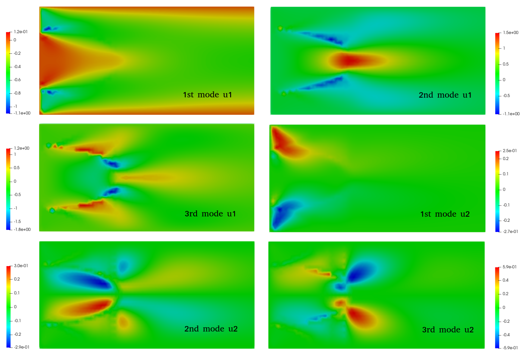
(a) First six modes for the velocity.

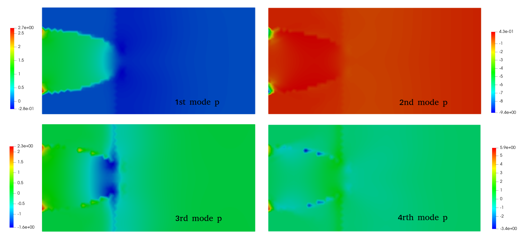
(b) First four modes for the pressure.

Figure 5. Steady system: Some reduced basis modes for velocity and pressure for a geometrically patrametrized Navier–Stokes system.

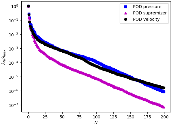
Figure 6. Steady case: POD eigenvalues decay for the fluid velocity u (black), the fluid pressure $p$ (blue), and the fluid supremizer s (magenta), for a set of $N_{train}=200$ snapshots.

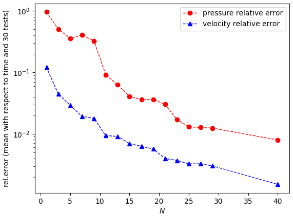
Figure 7. Steady case: Mode dependent errors between high fidelity and reduced order approximation, with the supremizer enrichment.

Figures 5(a) and 5(b) give an example of the first modes that we obtain with this procedure, whereas in Figure 6 we report the decay of the eigenvalues for all the components of the solution and for the supremizer. To test the reduced order model we generate randomly $N_{\text{test}}=30$ uniformly distributed values values for $\theta\in\mathcal{P}_{\text{test}}$. We are interested in the behavior of the relative approximation error that we obtain by changing the number of basis functions $N$ used to build the reduced solution. In order to do this we let $N$ vary in a discrete set $\mathcal{N}$: for a fixed value of $N\in\mathcal{N}$, and for each $\theta^{i}$, $i=1,\dots,N_{\text{test}}$, we compute both the reduced solution $(\bm{u}_{N}(\theta^{i}),p_{N}(\theta^{i}))$ and the corresponding full order solution $(\bm{u}_{h}(\theta^{i}),p_{h}(\theta^{i}))$. We compute the $L^{2}$ relative error $\epsilon_{u}^{N,i}$ for the velocity and the relative error $\epsilon_{p}^{N,i}$ for the pressure; then we compute the average approximation errors $\overline{\epsilon}_{u}^{N}$ and $\overline{\epsilon}_{p}^{N}$ for every $N\in\mathcal{N}$, defined as:

$$\overline{\epsilon}_{u}^{N}=\frac{1}{N_{\text{test}}}\sum_{i=1}^{N_{\text{test}}}\epsilon_{u}^{N,i}.$$

Figure 7 shows the relative approximation errors plotted against the number $N$ of basis functions used, with the use of the supremizer enrichment at the reduced order level.

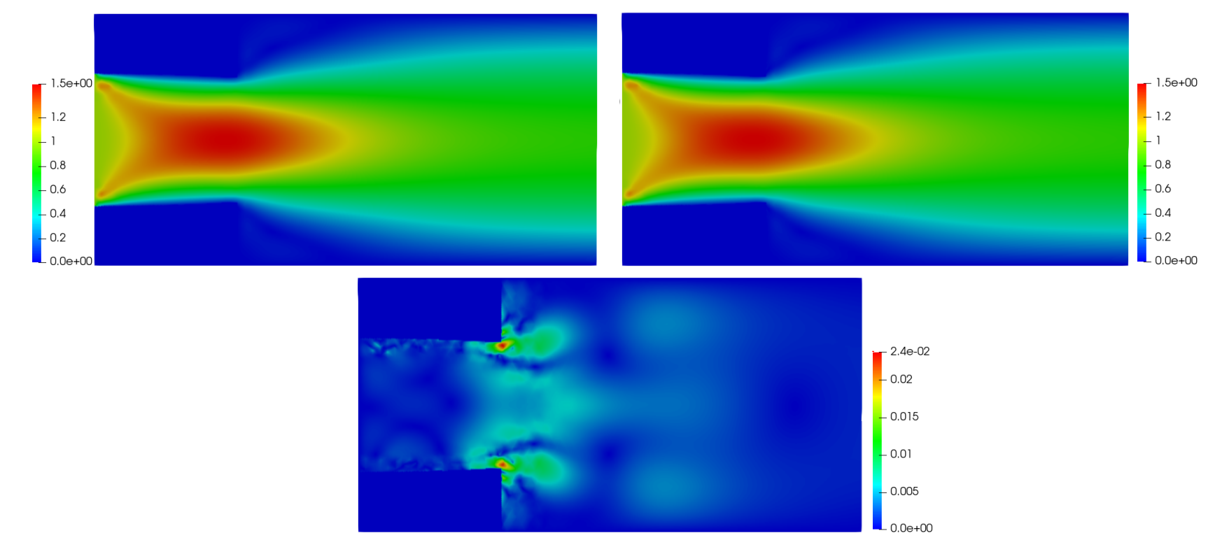
Figure 8. Steady case: Uncut geometry and the high fidelity velocity solution for parameter $\theta=-0.015854$ (left), reduced order solution for the same $\theta$ (right) and approximation error (middle)

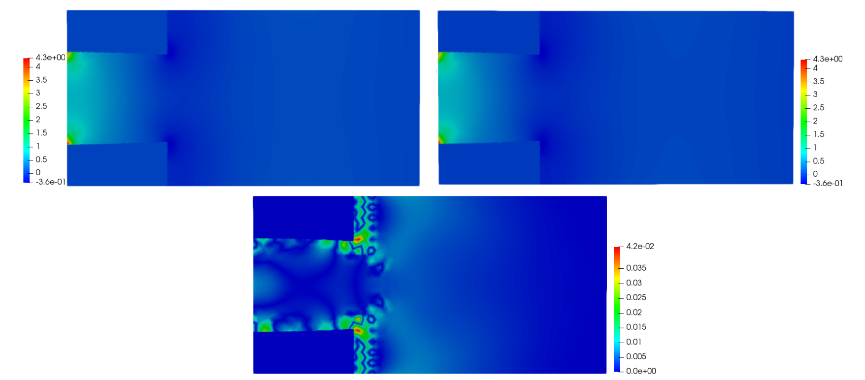
Figure 9. Steady case: Uncut geometry and the high fidelity pressure solution for parameter $\theta=-0.015854$ (left), reduced order solution for the same $\theta$ (right) and approximation error (middle)

Figures 8 and 9 show the approximation error for the velocity and pressure, for a given test value of the parameter, with the supremizer enrichment. It is worth to mention that the approximation error tends to concentrate near the cut between the physical domain and the background mesh, similar to to experiments in the works of [39, 41, 43, 40], phenomenon which will be studied in a future work.

3.5.1. Integration over boundary elements

The simulations presented in this manuscript have been implemented with ngsxfem, which is an add-on library to the finite element package Netgen/NGSolve, which enables the use of unfitted finite element technologies, such as CutFEM indeed. One of the main tools of ngsxfem is the availability of a routine that ”studies” the topology of the domain, identifying elements of the background mesh that are situated inside or outside the levelset function, or are cut-elements. Thanks to this routine, ngsxfem then takes automatically care of the integration of bilinear forms over cut-elements.

4. Unsteady Navier–Stokes

We now extend the previous treatment to the unsteady incompressible Navier–Stokes problem, by introducing the time evolution term $\partial_{t}{\bm{u}}(\theta)$ in system (1). The physical domain over which the problem is formulated is always the one in Figure 3.

4.1. Strong formulation

Given a time interval of interest $[0,T]$, the strong formulation of the problem reads as follows: for every $\theta\in\mathcal{P}$, and for every $t\in[0,T]$, find $\bm{u}(t;\theta)\colon\Omega(\theta)\mapsto\mathbb{R}^{2}$ and $p(t;\theta)\colon\Omega(\theta)\mapsto\mathbb{R}$ such that:

(12) $$\begin{cases}\partial_{t}{\bm{u}}(\theta)-\mu\Delta\bm{u}(\theta)+\nabla p(\theta)+(\bm{u}(\theta)\cdot\nabla)\bm{u}(\theta)=\bm{f}(\theta)\quad\text{in $\Omega(\theta)\times[0,T]$},\\ \text{div}\bm{u}(\theta)=0\quad\text{in $\Omega(\theta)\times[0,T]$},\\ \bm{u}(\bm{x},0;\theta)={\bm{u}}^{0}(\bm{x},\theta)\quad\text{in $\Omega(\theta)$},\end{cases}$$

with geometrical parameterization identical to that in the previous subsection. The problem is completed by the following boundary conditions: a prescribed inlet velocity $\bm{u}_{in}$ at the inlet boundary $\Gamma_{in}(\theta)$, a zero outflow condition at the outflow boundary, a boundary condition $\bm{u}(\theta)\cdot\bm{n}_{D}=0$ on $\Gamma_{D}$ and a no–slip boundary condition onf $\Gamma_{\theta}$.

4.2. Space discretization and time–stepping scheme

We discretize in time by a backwards Euler approach: we discretize the time interval $[0,T]$ with the following partition:

$${0=t^{0}<\ldots<t^{N_{t}}=T},$$

where every interval $(t^{n},t^{n+1}]$ has measure $\tau_{n+1}=t^{n+1}-t^{n}$, $n=0,...,N_{t}-1$. The discrete version of the initial condition $\bm{u}^{0}(x;\theta)$ is denoted by $\bm{u}^{0}_{h}(x;\theta)$; we denote $\bm{u}_{h}^{n}$ the discrete fluid velocity at time step $t^{n}$, and similar notation is used for the pressure.

After having applied a time stepping scheme, the space discretized weak formulation of the problem reads as follows: for every $n=0,\ldots,N_{t}-1$, we seek a discrete velocity ${\bm{u}}_{h}^{n+1}(\theta)\in V_{h,2}^{D}(\theta)$ and discrete pressure $p_{h}^{n+1}(\theta)\in Q_{h,1}(\theta)$, such that for every $(\bm{v}_{h}(\theta),q_{h}(\theta))\in V_{h,2}^{0}(\theta)\times Q_{h,1}(\theta)$, it holds:

$$m(\bm{u}_{h}^{n+1}(\theta)-\bm{u}_{h}^{n}(\theta),v_{h})+\tau_{n+1}\mathcal{A}(\bm{u}_{h}^{n+1}(\theta),p_{h}^{n+1}({\theta}),\bm{v}_{h}(\theta),q_{h}(\theta))=\tau_{n+1}\mathcal{L}(\bm{v}_{h}(\theta)),$$

where

$$m(\bm{w}_{h},\bm{v}_{h}):=\int_{\Omega(\theta)}\bm{w}_{h}\cdot\bm{v}_{h}\,dx,$$

where $\mathcal{L}(\bm{v}_{h}(\theta))$ is defined as in Section 3.2, and $\mathcal{A}({\bm{u_{h}}}^{n+1}(\theta),p_{h}^{n+1}(\theta),\bm{v_{h}}(\theta),q_{h}(\theta))$ is defined as follows:

$$\mathcal{A}(\bm{u}_{h}(\theta),p_{h}(\theta);\bm{v}_{h}(\theta),q_{h}(\theta)) = {a_{h}(\bm{u}_{h}(\theta),\bm{v}_{h}(\theta))+b_{h}(p_{h}(\theta),\bm{v}_{h}(\theta))-b_{h}(q_{h}(\theta),\bm{u}_{h}(\theta))+}$$

$${+c_{h}(\bm{u}_{h}(\theta);\bm{u}_{h}(\theta),\bm{v}_{h}(\theta)+{g}_{u}^{GP}(\bm{u}_{h}(\theta);\bm{u}_{h}(\theta),\bm{v}_{h}(\theta))+g_{\mu}^{GP}(\bm{u}_{h}(\theta),\bm{v}_{h}(\theta))+}$$

$${g_{\sigma}^{GP}(\bm{u}_{h}(\theta),\bm{v}_{h}(\theta))+g_{p}^{GP}(\bm{u}_{h}(\theta);p_{h}(\theta),q_{h}(\theta))}$$

The forms $a_{h}$, $b_{h}$, $c_{h}$ as well as the stabilization terms ${g}_{u}^{GP}$, $g_{\mu}^{GP}$, $g_{\beta}^{GP}$ and $g_{p}^{GP}$ have been introduced in Section 3.2.

4.3. POD and reduced basis generation

Similarly to what has been done in the previous Section 3.3, in the time dependent case an offline/online procedure will be employed, that will lead to the generation of a proper reduced basis set. Since the system is both (geometrical) parameter and time-dependent, we sample not only the geometrical parameter $\theta$, but also the time $t$, with the sample points $t^{k}\in\{t^{0},\dots,t^{N_{t}}\}\subset[0,T]$. This procedure is computationally more expensive and results in a much larger total number of snapshots to be collected with respect to the static system: the total number of snapshots that we collect is now equal to $\widehat{M}=M\cdot N_{t}$. The snapshots matrices $\bm{\mathcal{S}_{u}}$, $\bm{\mathcal{S}_{s}}$ and $\bm{\mathcal{S}}_{p}$ are then given by:

(13) $$\bm{\mathcal{S}}_{u}=[\hat{{\bm{u}}}^{0}_{h}(\theta^{1},t^{0}),\dots,\hat{{\bm{u}}}^{0}_{h}(\theta^{1},t^{N_{t}}),\dots,\hat{{\bm{u}}}^{0}_{h}(\theta^{M},t^{0}),\dots,\hat{{\bm{u}}}^{0}_{h}(\theta^{M},t^{N_{t}})]\in\mathbb{R}^{N_{u}^{h}\times\widehat{M}},$$

(14) $$\bm{\mathcal{S}}_{s}=[\hat{{\bm{s}}}_{h}(\theta^{1},t^{0}),\dots,\hat{{\bm{s}}}_{h}(\theta^{1},t^{N_{t}}),\dots,\hat{{\bm{s}}}_{h}(\theta^{M},t^{0}),\dots,\hat{{\bm{s}}}_{h}(\theta^{M},t^{N_{t}})]\in\mathbb{R}^{N_{u}^{h}\times\widehat{M}},$$

(15) $$\bm{\mathcal{S}}_{p}=[\hat{{p}}_{h}(\theta^{(1)},t^{0}),\dots,\hat{{p}}_{h}(\theta^{1},t^{N_{t}}),\dots,\hat{{p}}_{h}(\theta^{M},t^{0}),\dots,\hat{{p}}_{h}(\theta^{M},t^{N_{t}})]\in\mathbb{R}^{N_{p}^{h}\times\widehat{M}},$$

where we used the $\hat{}$ notation to indicate that we implemented, also in this case, a natural smooth extension of the FE solutions obtained in the offline phase of the method, in order to work with parameter–independent reduced basis functions and parameter–independent reduced basis spaces, as well as a lifting function for the inlet velocity, see Section 3.3.1. We solve an eigenvalue problem like the one introduced in Section 3.3, and finally, adopting the notation of Section 3.4 we end up with the parameter–independent reduced basis spaces

$$\hat{V}_{N}=\text{span}\{\bm{\Phi}_{1}^{u,s},\ldots,\bm{\Phi}_{2N}^{u,s}\},\qquad\hat{Q}_{N}=\text{span}\{\Phi_{1}^{p},\ldots,\Phi_{N}^{p}\},$$

Let us now denote by $(\bm{u}_{N}^{n}(\theta),p_{N}^{n}(\theta))$ the reduced solution at time-step $t^{n}$, for $n=0,\ldots,N_{t}$, where $\bm{u}_{N}^{n}(\theta):=\bm{u}_{N}^{n,0}(\theta)+\ell(\theta)$, and $\bm{u}_{N}^{n,0}(\theta)$ and $p_{N}^{n}(\theta)$ are defined as in (9) and in (10), respectively. We can derive the subsequent reduced algebraic system for the unknown $U_{h}^{n+1}(\theta)=(\bm{u}_{N}^{n+1,0}(\theta),p_{N}^{n+1}(\theta))$:

(16) $$\begin{bmatrix}{\bm{L}_{u,s}^{T}\hat{\bm{M}}\bm{L}_{u,s}}&\bm{0}\\ \bm{0}&\bm{0}\end{bmatrix}U_{N}^{n+1}(\theta)+\tau_{n+1}\hat{R}_{N}(U_{N}^{n+1}(\theta);\theta)=\begin{bmatrix}{{\bm{L}_{u,s}^{T}\hat{\bm{M}}\bm{L}_{u,s}}}&\bm{0}\\ \bm{0}&\bm{0}\end{bmatrix}U_{N}^{n}(\theta),$$

where $\hat{M}_{ij}:=(\hat{\bm{\varphi}}^{i},\hat{\bm{\varphi}}^{j})_{\mathcal{R}}$. Here $\{\hat{\bm{\varphi}}^{i}\}_{i=1}^{N_{u}^{h}}$ are the FE basis functions of the FE parameter–independent spaces $\hat{V}_{h,2}^{D}$ and $\hat{Q}_{h,1}$, as defined in Section 3.3.2. Here, $\hat{R}(U_{N}(\theta);\theta)$ is defined as in Section 3.4.

4.4. Numerical results

In this paragraph we present the results obtained by applying the proposed reduction technique to a time dependent case. The time-step used in our simulation is $\tau=0.011s$, and the final time is $T=0.7s$. The fluid viscosity is $\mu_{f}=0.05$ $cm^{2}/s$ and the fluid density is $1$ $g/cm^{3}$. We impose a constant inlet velocity $\bm{u}_{\text{in}}=(1,0)$ $m/s$. We now take $N_{\text{train}}=200$, and we generate randomly $N_{\text{train}}$ uniformly distributed values for the parameter $\theta$. We also remind that we sample the time interval $[0,T]$ with an equispaced sampling $\{t_{0},\ldots,t_{N_{t}}\}$. We then run a POD on the set of snapshots collected, and we obtain our basis functions with which we are going to compute the reduced solutions $(\bm{u}_{N}(t,\theta^{i}),p_{N}(t,\theta^{i})$, where $i=1,\dots,N_{\text{test}}$, and $N$ is the number of basis functions that we use.

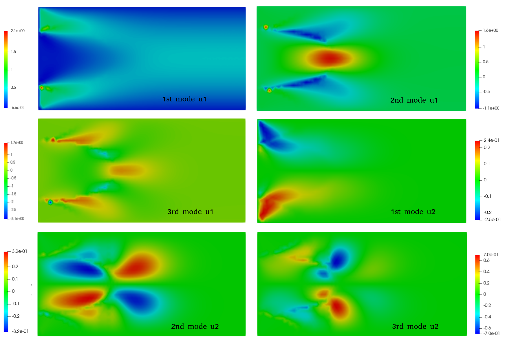
(a) First six modes for the velocity.

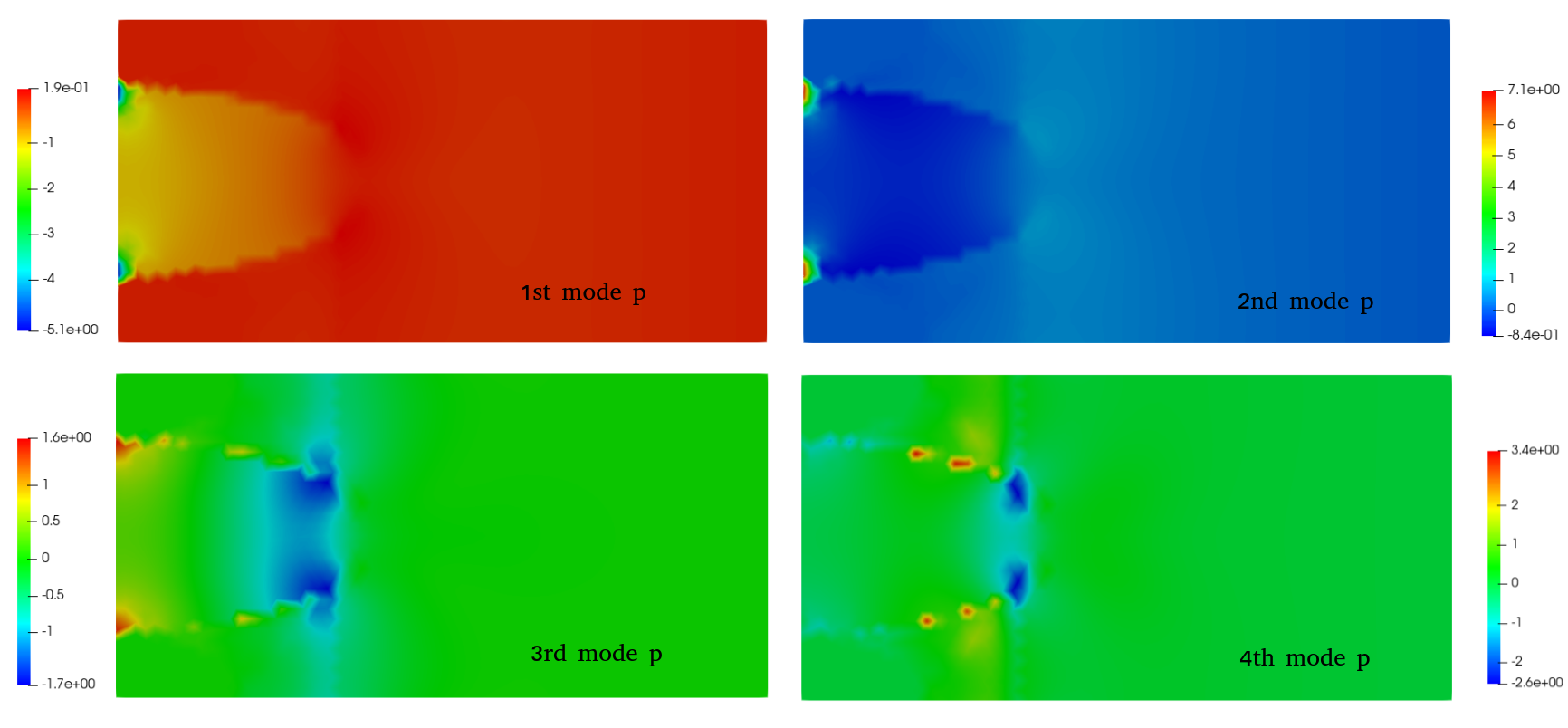
(b) First four modes for the pressure.

Figure 10. Unsteady system with static in time geometry: Some reduced basis modes for velocity and pressure for the evolutionary in time, geometrically patrametrized Navier–Stokes system.

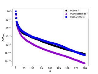
Figure 11. Time dependent case and the POD eigenvalues decay for the fluid velocity u (black), the fluid pressure $p$ (blue), and the fluid supremizer s (magenta), for a set of $N_{train}=200$ snapshots.

Figure 10 gives an example of the first modes that we obtain with this procedure, whereas in Figure 11 we show the rate of decay of the eigenvalues for all the components of the solution and for the supremizer. To test the reduced order model we generate randomly $N_{\text{test}}=30$ uniformly distributed values for $\theta\in\mathcal{P}_{\text{test}}$.
We are again interested in the behavior of the relative approximation error as a function of the number $N$ of basis functions used at the reduced order level. We therefore let $N$ vary in a discrete set $\mathcal{N}$: for a fixed value of $N\in\mathcal{N}$, and for each $\theta_{i}$, $i=1,\dots,N_{\text{test}}$, we compute both the reduced solution $(\textbf{u}_{N}(t,\theta^{i}),p_{N}(t,\theta^{i}))$ and the corresponding high order solution $(\bm{u}_{h}(t,\theta^{i}),p_{h}(t,\theta^{i}))$. We calculate the $L^{2}$ relative error $\epsilon_{u,t_{k}}^{N,i}$ for the velocity and the relative error $\epsilon_{p,t_{k}}^{N,i}$ for the pressure at time $t_{k}$, by taking an average of these relatives error we obtain the mean approximation error $\epsilon_{u}^{N,i}$ for $\bm{u}$ and $\epsilon_{p}^{N,i}$ for $p$, for each $\theta_{i}\in\mathcal{P}_{\text{test}}$. Finally we compute the average approximation errors $\overline{\epsilon}_{u}^{N}$ and $\overline{\epsilon}_{p}^{N}$ for every $N\in\mathcal{N}$, defined as:

$$\overline{\epsilon}_{u}^{N}=\frac{1}{N_{\text{test}}}\sum_{i=1}^{N_{\text{test}}}\epsilon_{u}^{N,i}.$$

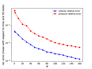
Figure 12. Unsteady case: Mode dependent errors between high fidelity and reduced order approximation, with the supremizer enrichment.

Figure 12 shows the relative approximation errors plotted against the number $N$ of basis functions used, with the supremizer enrichment at the reduced order level.

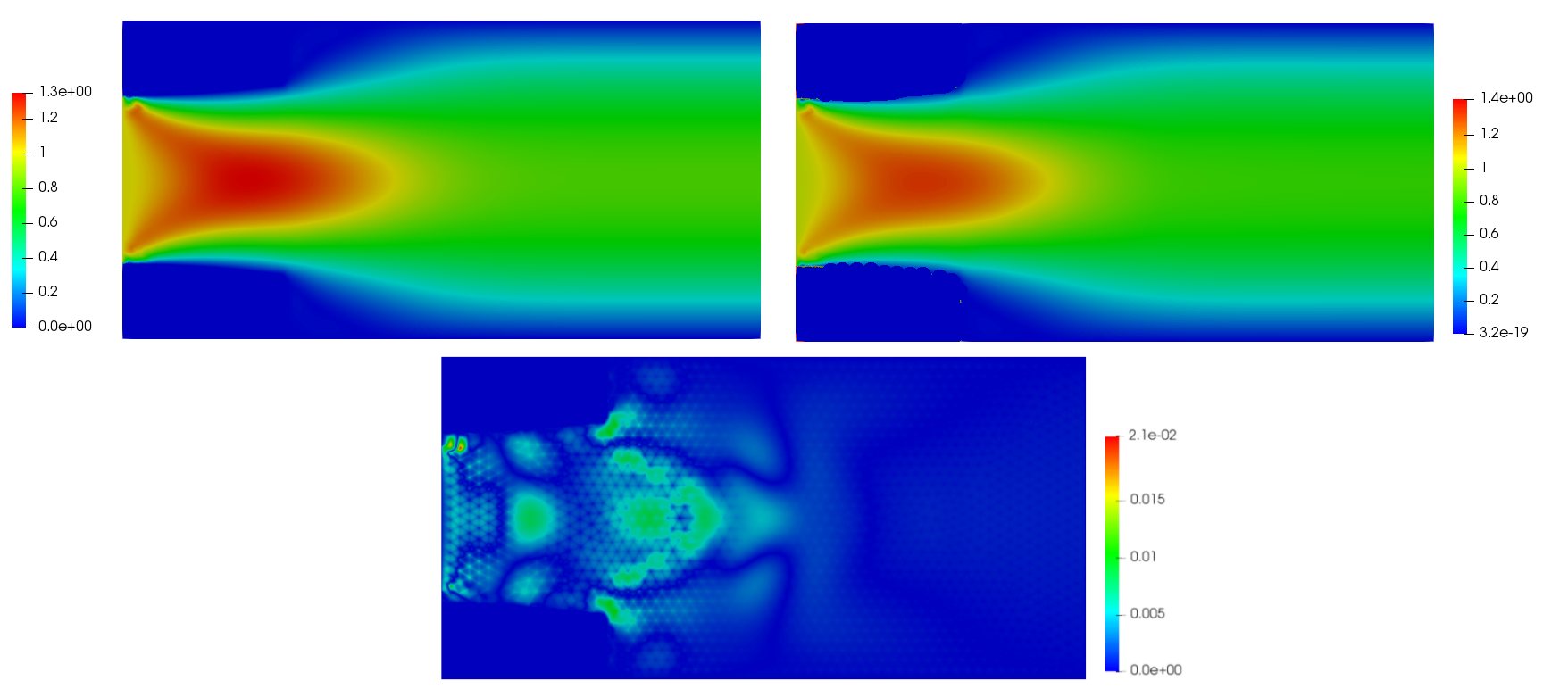
Figure 13. Unsteady case: Cut geometry and high fidelity fluid velocity at final time $T=0.7$ for parameter $\theta=0.045406$ (left), reduced order solution for the same $\theta$ (right) and approximation error (bottom).

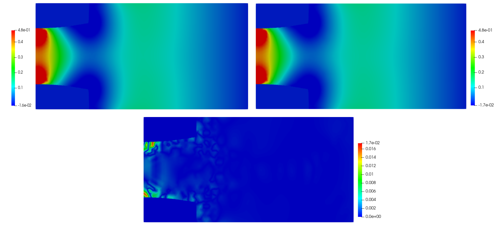
Figure 14. Unsteady case: Cut geometry and the high fidelity pressure solution at final time at final time $T=0.7$ for parameter $\theta=0.050014$ (left), reduced order solution for the same $\theta$ (right) and approximation error (bottom).

Figure 14 shows the approximation error for the pressure, for the same parameter value, with the supremizer enrichment. Figure 13 shows the approximation error for the fluid velocity $\bm{u}_{f}$ for a given value of the test parameter $\theta$, at the final time-step of the simulation.

5. Unsteady Navier–Stokes: immersed obstacle

We now consider here a further test case of interest, namely the case of an obstacle immersed in a fluid. For this test case we assume that $\mathcal{D}(\theta)$ represents a cylinder immersed in the fluid domain, and therefore we denote herein $\Gamma_{\theta}=\partial\mathcal{D}(\theta)$ the immersed boundary.

Figure 15. The physical domain of interest (light blue) and the levelset geometry (dark blue). The position of the immersed obstacle is determined by a geometrical parameter $\theta$. The immersed boundary is $\partial\mathcal{D}(\theta):=\Gamma_{\theta}$.

The physical domain over which the problem is formulated is depicted in Figure 15.

5.1. Strong formulation.

The problem reads as follows: for every $t\in[0,T]$ and for every $\theta\in\mathcal{P}\subset\mathbb{R}$, find $\bm{u}(t;\theta)\colon\Omega(\theta)\mapsto\mathbb{R}^{2}$, $p(t;\theta)\colon\Omega(\theta)\mapsto\mathbb{R}$ such that:

(17) $$\begin{cases}\partial_{t}\bm{u}(\theta)-\mu\Delta\bm{u}(\theta)+\nabla p(\theta)+(\bm{u}(\theta)\cdot\nabla)\bm{u}(\theta)=\bm{f}(\theta)\quad\text{in $\Omega(\theta)\times[0,T]$},\\ \text{div}\bm{u}(\theta)=0\quad\text{in $\Omega(\theta)\times[0,T]$},\\ \bm{u}(\bm{x},0;\theta)={\bm{u}}^{0}(\bm{x},\theta)\quad\text{in $\Omega(\theta)$}.\end{cases}$$

The previous system is completed by the following boundary conditions: a prescribed inlet velocity $\bm{u}_{in}$ at the inlet boundary $\Gamma_{in}$, a no slip boundary condition on the immersed boundary $\Gamma_{\theta}$, a zero outflow condition on $\Gamma_{out}$ and a boundary condition $\bm{u}(\theta)\cdot\bm{n}_{D}=0$ on $\Gamma_{D}$.

5.1.1. Geometrical parametrization

The obstacle immersed in the fluid domain in our problem is a circle, defined through the time dependent levelset function:

$$\phi(x,y,\theta)=(x+1.5)^{2}+(y-\theta)^{2}-R^{2},$$

where $\theta$ determines the position of the center of the cylinder in the domain, and $R$ is the radius of the circle.

Figure 16. Different levelset geometries: from left to right, $\theta=0.5$, $\theta=-0.5$, $\theta=0$.

Figure 16 shows the physical domain $\Omega(\theta)$ for different values of the parameter $\theta$: as we can see, changing the value of the geometrical parameter can produce a significant change in the physical domain of interest, and therefore this situation is particularly interesting for an unfitted discretization point of view, since adopting a standard discretization would require remeshing, or, alternatively, remapping the whole problem (17) onto a reference configuration, similarly to what is done for example with an Arbitrary Lagrangian Eulerian approach in fluid–structure interaction (see for example [46, 7, 49, 63]).

5.1.2. Weak formulation and time discretization

We now want to state the weak formulation of the original problem after discretization in space and after having applied a time stepping scheme. As far as the time discretization concerns, we employ the time stepping scheme adopted in Section 4: we discretize the time interval $[0,T]$ in sub-intervals $(t^{n},t^{n+1}]$ of measure $\tau_{n+1}=t^{n+1}-t^{n}$, for $n=0,\ldots,N_{t}-1$. Also in this case, we decide to treat the boundary conditions in the following way: the boundary conditions on $\Gamma_{D}$ and on $\Gamma_{out}$, as well as the condition on the inlet profile, are imposed strongly; only the boundary condition on the immersed boundary $\Gamma_{\theta}$ is imposed weakly, thanks to the Nitsche method. For the space discretization we therefore use the discrete spaces introduced in Section 4.2, and which we recall briefly:

$$\begin{split}V_{h,2}(\theta)&:=\{\bm{v}_{h}\in(C_{0}(\Omega^{*}_{h}(\theta)))^{2}\colon\bm{v}_{h}|_{T}\in(\mathcal{P}^{2}(T))^{2},\quad\forall T\in\mathcal{I}_{h}(\theta)\},\\ V_{h,2}^{D}(\theta)&:=\{\bm{v}_{h}\in V_{h,2}(\theta)\text{ such that }\bm{v}_{h}=\bm{u}_{in}\text{ on }\Gamma_{in}\text{ and }\bm{v}_{h}\cdot\bm{n}_{D}=0\text{ on }\Gamma_{D}\},\\ V_{h,2}^{0}(\theta)&:=\{\bm{v}_{h}\in V_{h,2}(\theta)\text{ such that }\bm{v}_{h}=\bm{0}\text{ on }\Gamma_{in}\text{ and }\bm{v}_{h}\cdot\bm{n}_{D}=0\text{ on }\Gamma_{D}\},\\ Q_{h,1}(\theta)&:=\{q_{h}\in C_{0}(\Omega^{*}_{h}(\theta))\colon q_{h}|_{T}\in\mathcal{P}^{1}(T),\quad\forall T\in\mathcal{I}_{h}(\theta)\}.\end{split}$$

For the weak formulation we restore to the one presented in Section 4.2.

5.2. Proper Orthogonal Decomposition and online system

Also in this case, once we have computed the snapshots $(\bm{u}_{h}(t^{i};\theta),p_{h}(t^{i};\theta))$, for all $\theta$ in a discrete parameter training set $\mathcal{P}_{train}$ and for $i=0,\dots,N_{t}$, we rely on a natural smooth extension of the snapshots, and on a lifting of the inlet boundary condition, in order to obtain solutions that are defined on the whole background mesh $\hat{\mathcal{I}}_{h}$. Again, we use a supremizer enrichment technique in order to obtain stable approximations of the pressure in the online step, and we use a lifting function to treat the non–homogeneous Dirichlet condition at the inlet boundary $\Gamma_{in}$. Also here, in order to make the notation more light, we will omit the lifting function, with the understanding that it has been used for implementation purposes. After having created the parameter independent reduced basis functions $\{\bm{\Phi}_{i}^{u,s}\}_{i=1}^{2N}$ and $\{\Phi_{i}^{p}\}_{i=1}^{N}$ for the fluid velocity and fluid pressure respectively, the online algebraic system that we are going to solve, for every $\theta\in\mathcal{P}$, is the one presented in Equation (16):

$$\begin{bmatrix}{\bm{L}_{u,s}^{T}\hat{\bm{M}}\bm{L}_{u,s}}&\bm{0}\\ \bm{0}&\bm{0}\end{bmatrix}U_{N}^{n+1}(\theta)+\tau_{n+1}\hat{R}_{N}(U_{N}^{n+1}(\theta);\theta)=\begin{bmatrix}{{\bm{L}_{u,s}^{T}\hat{\bm{M}}\bm{L}_{u,s}}}&\bm{0}\\ \bm{0}&\bm{0}\end{bmatrix}U_{N}^{n}(\theta).$$

5.3. Numerical results

We now present some numerical results for the test case of the immersed obstacle. The cylinder has a radius $R=0.2$ $cm$, and the center C of the cylinder has coordinates $(x_{c},y_{c})=(-1.5,\theta)$, with $\theta\in[-0.65,0.65]$. The background domain $\mathcal{R}$ is a rectangle of coordinates $(-2,-1)$ and $(2,1)$. The fluid viscosity is $\mu=0.05$, the fluid density is $1$. The mesh size is $h_{max}=0.07$, and the timestep used for the discretization is $\tau=\frac{h_{max}}{6}$; the final time of the simulation is $T=0.7$ $s$. The inlet velocity profile is $u_{in}=(1,0)$ $m/s$. In this case, $N_{train}=200$ is the number of parameters $\theta^{i}$ that we take to compute the snapshots for the POD, whereas $N_{test}=30$ is the number of parameters $\theta^{i}$ for which we compute the online solution.

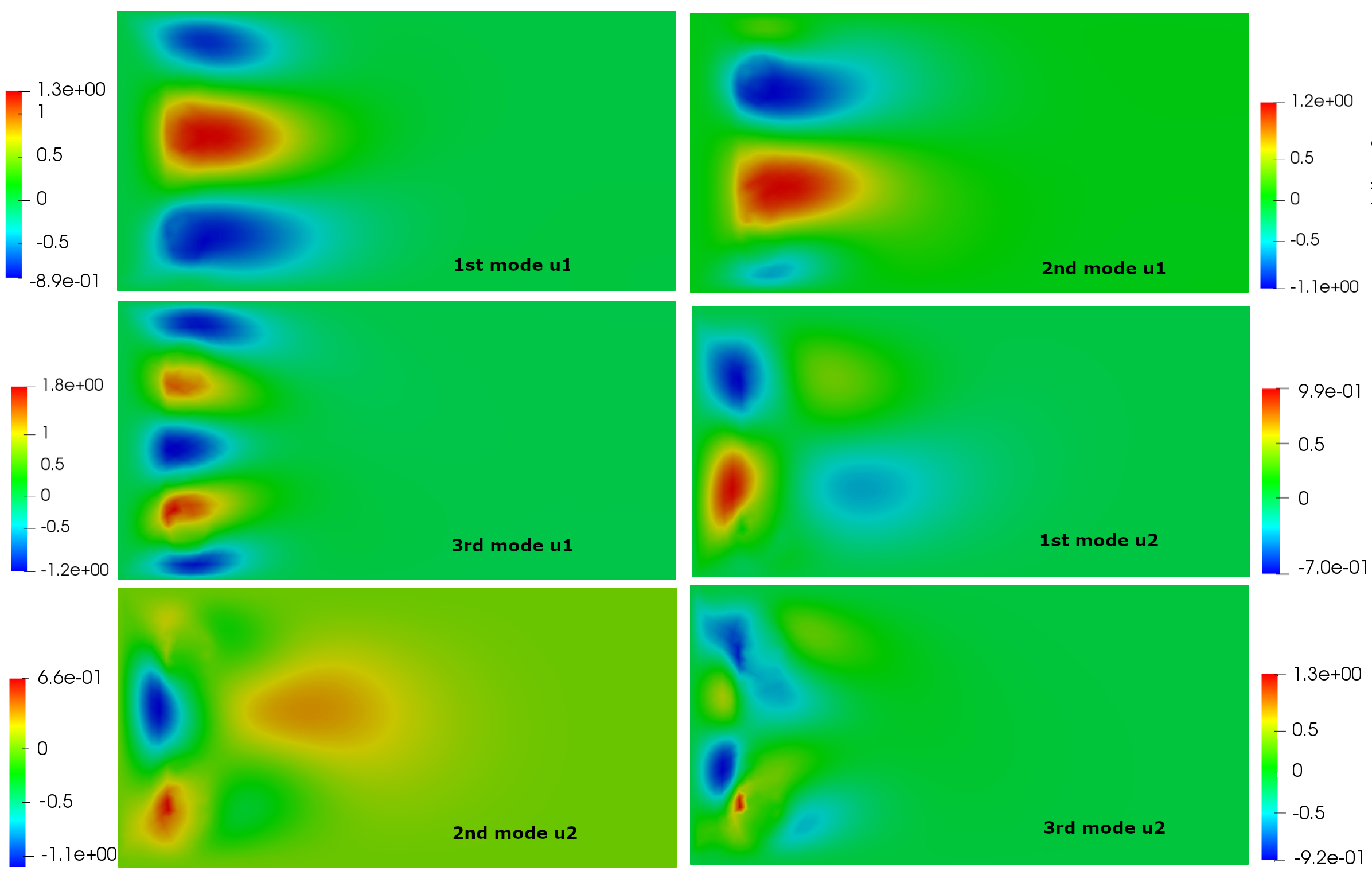
Figure 17. First three modes for the $x$–component of the velocity and for the $y$–component.

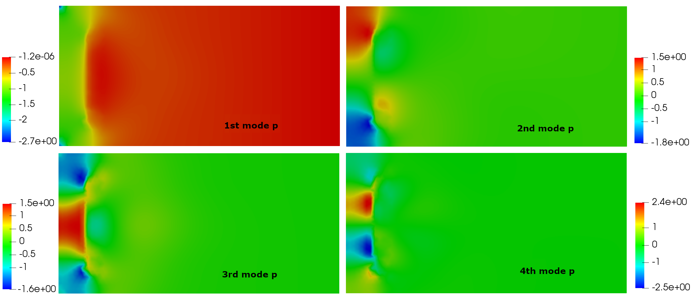
Figure 18. First four pressure modes

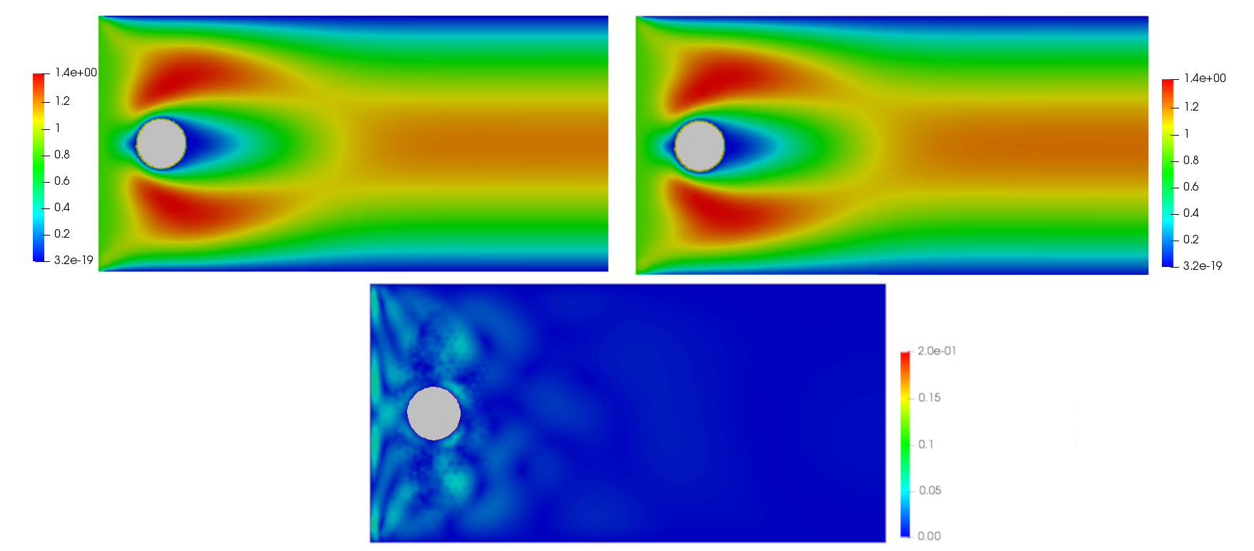
Figure 19. Fluid velocity approximation (top left), reduced order approximation (top right) and approximation error (bottom), for $\theta=0$, at time $t=0.7$ s.

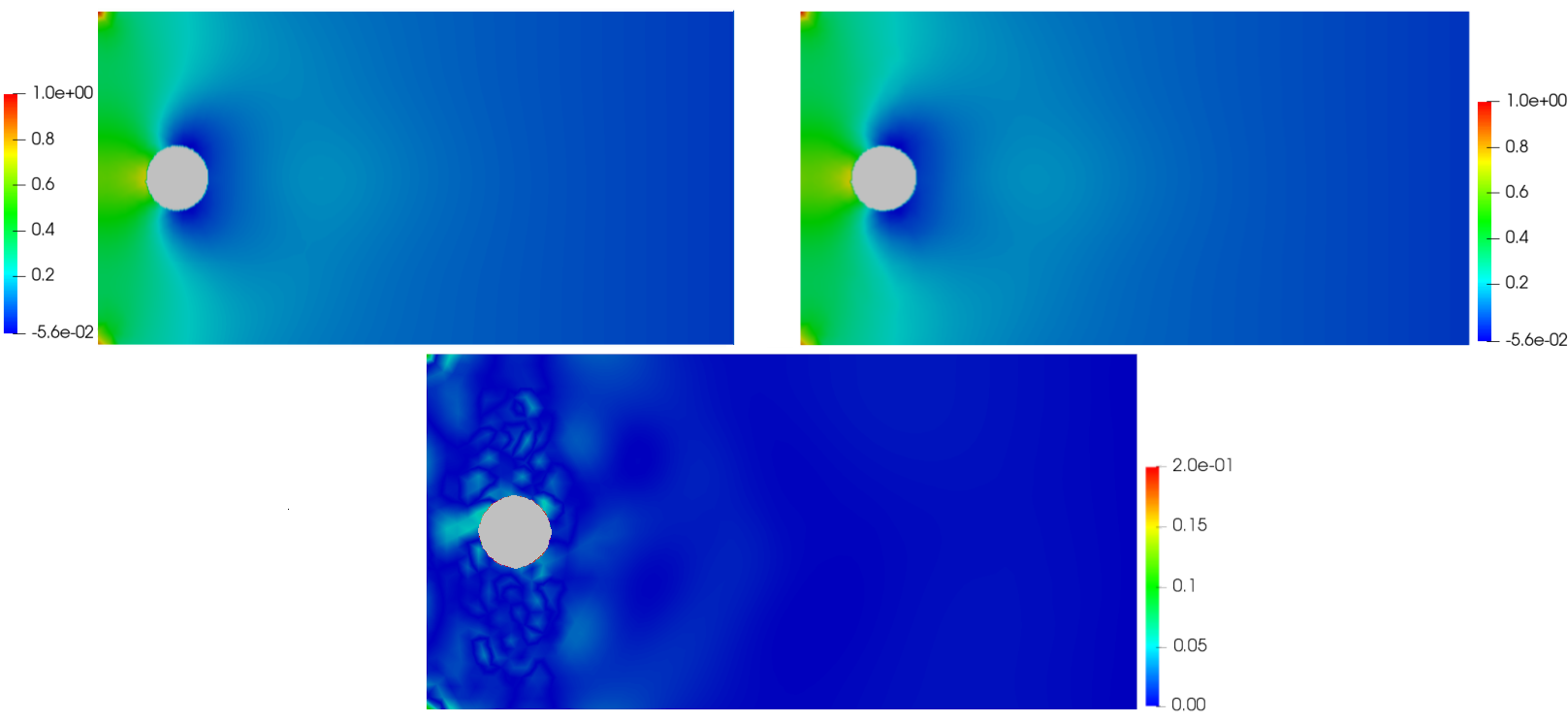
Figure 20. Pressure approximation (top left), reduced order approximation (top right) and approximation error (bottom), for $\theta=0$, at time $t=0.7$ s.

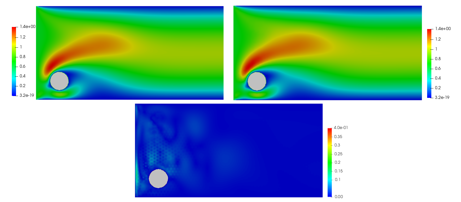
Figure 21. Fluid velocity approximation (top left), reduced order approximation (top right) and approximation error (bottom), for $\theta=0.6$, at time $t=0.7$ s.

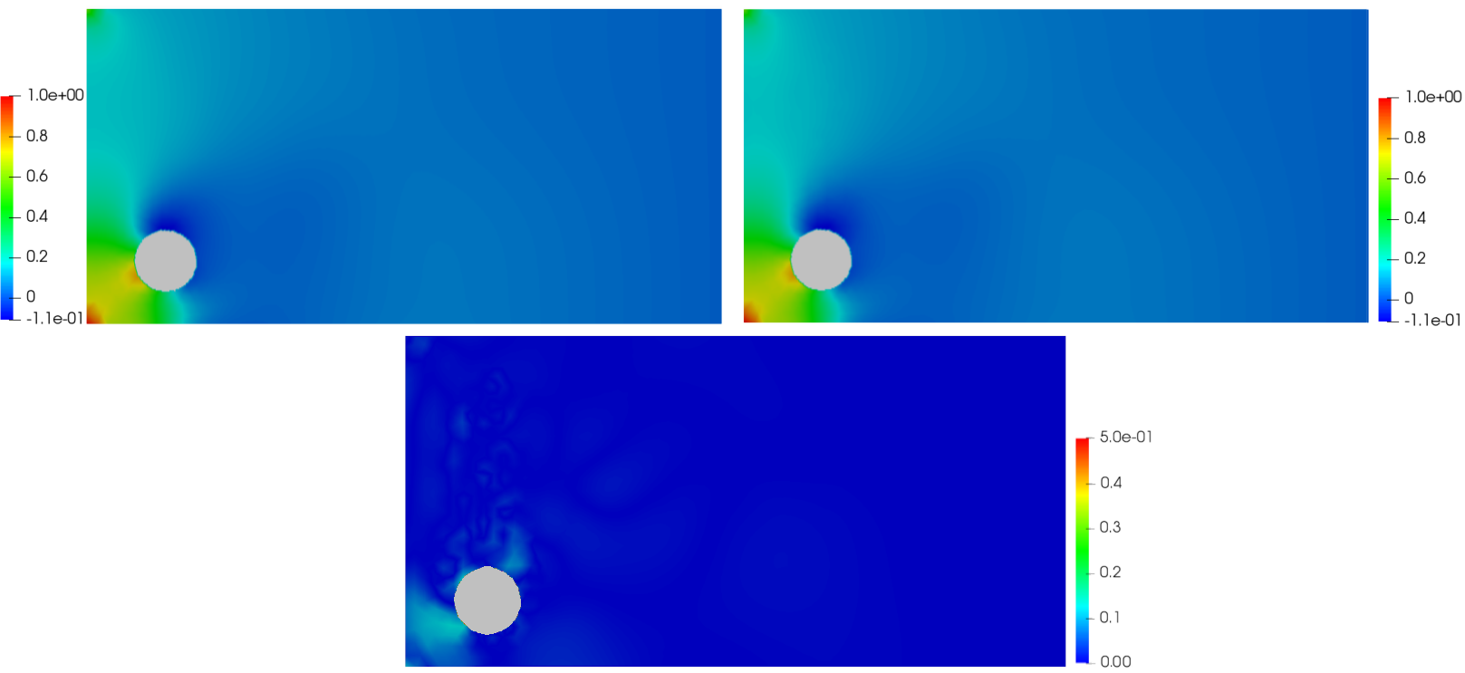
Figure 22. Pressure approximation (top left), reduced order approximation (top right) and approximation error (bottom), for $\theta=0.6$, at time $t=0.7$ s.

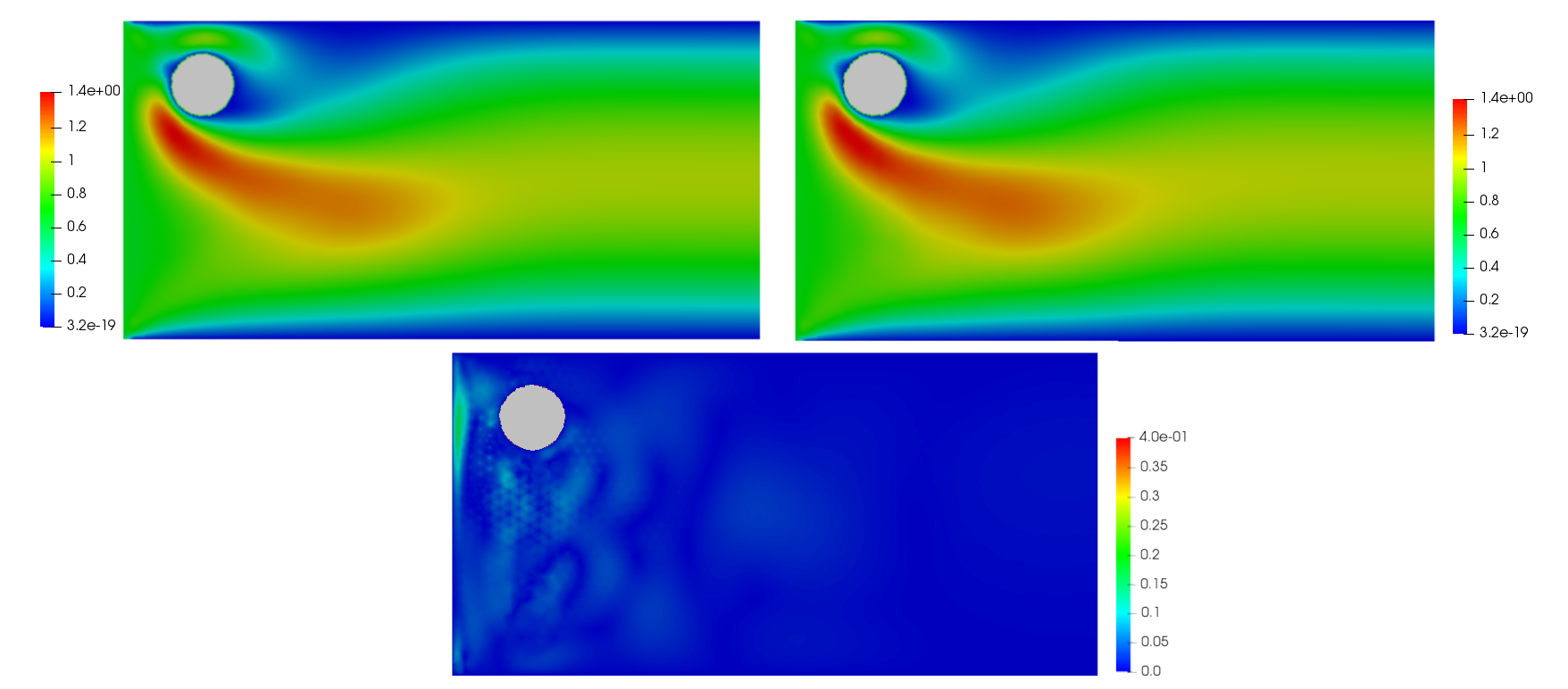
Figure 23. Fluid velocity approximation (top left), reduced order approximation (top right) and approximation error (bottom), for $\theta=-0.6$, at time $t=0.7$ s.

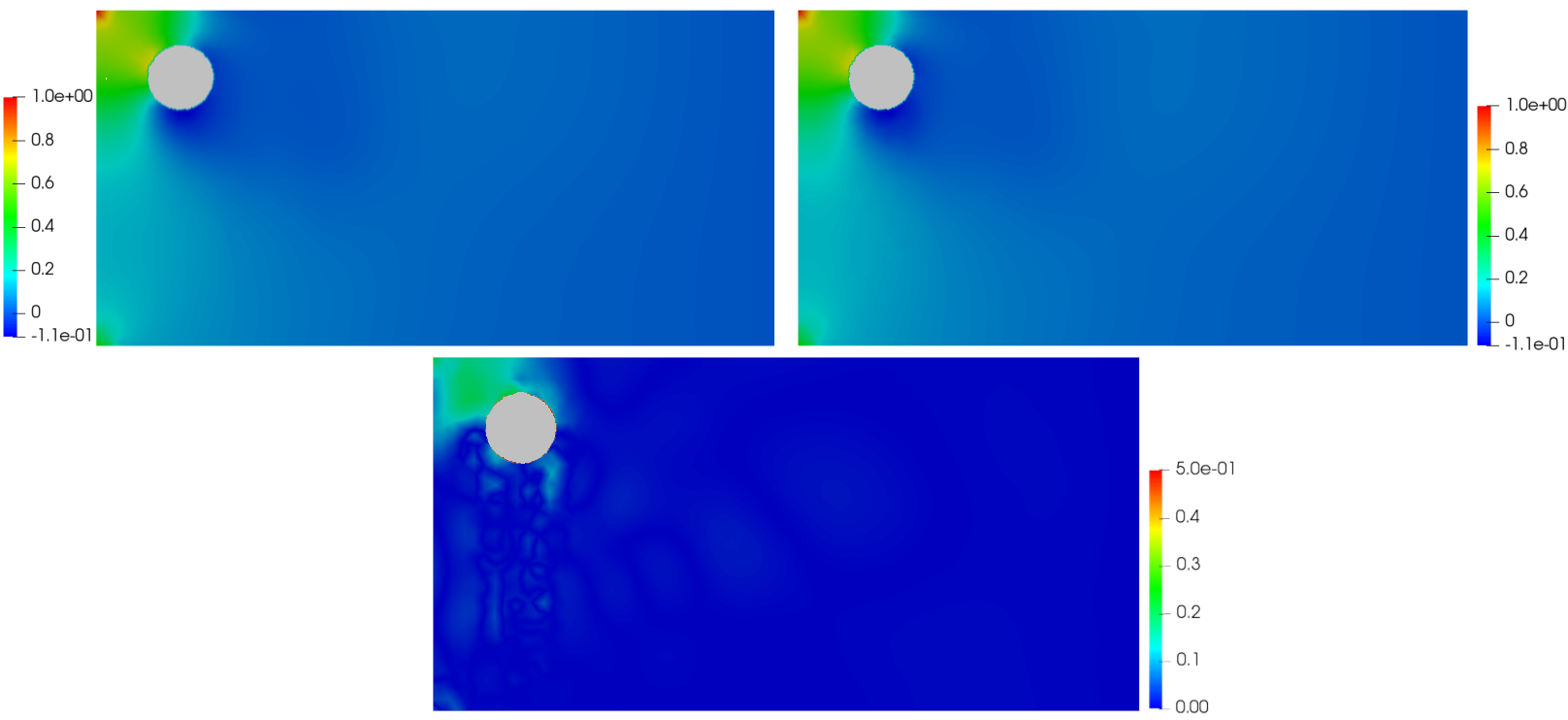
Figure 24. Pressure approximation (top left), reduced order approximation (top right) and approximation error (bottom), for $\theta=-0.6$, at time $t=0.7$ s.

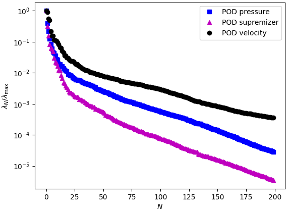
Figure 25. Immersed obstacle: decay of the first $200$ eigenvalues returned by the POD on the fluid velocity (black), the pressure (magenta) and the supremizer (blue).

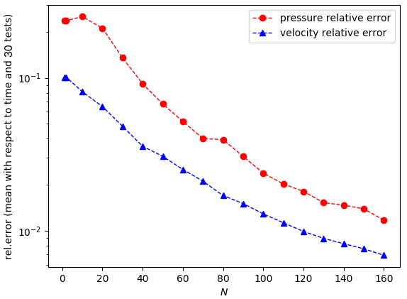
Figure 26. Immersed obstacle: mean error behaviour, according to different number of basis functions used in the online phase, for the fluid velocity (blue) and the pressure (red). The results were obtained using the supremizer enrichment technique.

Figures 19–24 represent the fluid velocity and the fluid pressure, at the last time-step of the simulation, for three different values of the geometrical parameter $\theta$. As we can see, the change in the position of the immersed obstacle, according to the parameter $\theta$, is significant; nonetheless, with an unfitted discretization we were able to obtain very good results, in terms of both velocity and pressure approximation. The use of the supremizer enrichment technique helps to obtain a more accurate results for the reduced order fluid pressure. In Figure 25 we can see the behaviour of the first eigenvalues returned by a POD on the fluid velocity, the fluid pressure and the fluid supremizer; Figure 26 shows the behaviour of the mean approximation error, plotted against the number $N$ of basis functions used for the online approximation, and for $30$ values of the parameter $\theta$ in the test sample. We remark that these results have been obtained without the implementation of any snapshot transportation technique (see for example [39, 46, 22]): the analysis of the influence of this additional feature on the overall quality of the approximation at the reduced order level is left for a future work.

6. Conclusions

In this work we have introduced a POD–Galerkin ROM approach for geometrically parametrized two dimensional Navier–Stokes equations, both in the steady and in the unsteady case. The procedure that we have proposed shows many of the advantages that characterize CutFEM and reduced order methods. First of all, by choosing an unfitted mesh approach, we have shown that it is possible to work with geometries that can potentially change significantly the shape of (part of) the domain, as we can see from the examples in Figure 4 and Figure 16. By employing an unfitted CutFEM approach at the full order level, we can let the geometrical parameter $\theta$ vary in a large interval of values: this helps to overcome one of the limitations of the standard Finite Element discretization, where a re–meshing would have been needed.

At the reduced order level, an unfitted mesh discretization has been combined with a snapshot extension, in order to be able to work with finite dimensional spaces that are parameter–independent: the importance of this aspect is related to the choice of performing a Proper Orthogonal Decomposition. In addition, the implementation of a supremizer enrichment technique allows us to obtain a stable approximation of the fluid pressure. Combined together, the unfitted CutFEM discretization and the Reduced Basis Method represent a very powerful tool, which here allowed us to investigate time–dependent, nonlinear fluid flows problems. To conclude, with this work we started to prepare the basis for a CutFEM-RB procedure that, thanks to a Galerkin projection and with the use of a supremizer enrichment, will ideally be used to obtain accurate approximations of solutions of very complex problems, such as fully coupled multiphysics problem, where large displacements of the structure may occur. Therefore, as future perspectives, we first would like to extend the procedure presented here to nonlinear, time–dependent problems, where the levelset geometry is time–dependent (i.e. the motion of the levelset geometry is time–dependent, and this motion is known a priori); then, we would like to move to a more general case, where on the contrary the motion of the levelset geometry is an unknown of the problem. As a next step and as final goal therefore, we would like to test the performance of this approach with time dependent Fluid–Structure Interaction problems, geometrically shallow water flows as well as with phase flow Navier-Stokes systems. Furthermore, from the model reduction point of view, we will pursue further developments in hyper-reduction techniques [64, 9, 24, 61] tailored for unfitted discretizations.

References

- [1] ngsxfem – Add-On to NGSolve for unfitted finite element discretizations, https://github.com/ngsxfem/ngsxfem.
- [2] RBniCS - reduced order modelling in FEniCS, https://www.rbnicsproject.org, 2015.
- [3] NGSolve - high performance multiphysics finite element software, https://github.com/NGSolve/ngsolve, 2018.
- [4] I. Akhtar, A. Nayfeh, and C. Ribbens, On the stability and extension of reduced-order Galerkin models in incompressible flows, Theoretical and Computational Fluid Dynamics 23 (2009), no. 3, 213–237.
- [5] M. Balajewicz and C. Farhat, Reduction of nonlinear embedded boundary models for problems with evolving interfaces, Journal of Computational Physics 274 (2014), 489–504.
- [6] F. Ballarin, A. Manzoni, A. Quarteroni, and G. Rozza, Supremizer stabilization of POD-Galerkin approximation of parametrized steady incompressible Navier–Stokes equations, International Journal for Numerical Methods in Engineering 102 (2015), no. 5, 1136–1161.
- [7] F. Ballarin and G. Rozza, POD–Galerkin monolithic reduced order models for parametrized fluid-structure interaction problems, International Journal for Numerical Methods in Fluids 82 (2016), no. 12, 1010–1034.
- [8] F. Ballarin, G. Rozza, and Y. Maday, MS&A, vol. 17, ch. Reduced-order semi-implicit schemes for fluid–structure interaction problems, pp. 149–167, Springer International Publishing, Cham, 2017.
- [9] M. Barrault, Y. Maday, N. Nguyen, and A. Patera, An ‘empirical interpolation’ method: application to efficient reduced-basis discretization of partial differential equations, Comptes Rendus Mathematique 339 (2004), no. 9, 667–672.
- [10] R. Becker, Mesh adaptation for dirichlet flow control via nitsche’s method, Communications in Numerical Methods in Engineering 18 (2002), no. 9, 669–680.
- [11] R. Becker, E. Burman, and P. Hansbo, A Nitsche extended finite element method for incompressible elasticity with discontinuous modulus of elasticity, Computer Methods in Applied Mechanics and Engineering 198 (2009), 3352–3360.
- [12] P. Benner, M. Ohlberger, A. Patera, G. Rozza, and K. Urban, Model Reduction of Parametrized Systems, MS&A series, vol. 17, Springer, 2017.
- [13] M. Bergmann, C.-H. Bruneau, and A. Iollo, Enablers for robust POD models, Journal of Computational Physics 228 (2009), no. 2, 516–538.
- [14] D. Boffi, F. Brezzi, and M. Fortin, Mixed Finite Element Methods and Applications, 1 ed., Springer-Verlag Berlin Heidelberg, (2013).
- [15] E. Burman, Interior penalty variational multiscale method for the incompressible Navier–Stokes equation: monitoring artificial dissipation, Computer Methods in Applied Mechanics and Engineering 196 (2007), no. 41, 4045 – 4058.
- [16] E. Burman, Ghost penalty, Comptes Rendus Mathematique 348 (2010), no. 21, 1217–1220.
- [17] by same author, A penalty–free nonsymmetric nitsche type method for the weak imposition of boundary conditions, SIAM Journal of Numerical Analysis 50 (2012), 1959–1981.
- [18] E. Burman, S. Claus, P. Hansbo, M. Larson, and A. Massing, CutFEM: discretizing geometry and partial differential equations, International Journal for Numerical Methods in Engineering 104 (2014), 472–501.
- [19] E. Burman and M. A. Fernández, Continuous interior penalty finite element method for the time-dependent Navier–Stokes equations: space discretization and convergence, Numerische Mathematik 107 (2007), 39–77.
- [20] E. Burman and P. Hansbo, Fictitious domain finite element methods using cut elements: II. A stabilized Nitsche method, Applied Numerical Mathematics 52 (2011), no. 6, 2837–2862.
- [21] E. Burman and P. Hansbo, Fictitious domain methods using cut elements: III. a stabilized Nitsche method for Stokes’ problem, ESAIM: Mathematical Modelling and Numerical Analysis - Modélisation Mathématique et Analyse Numérique 48 (2014), no. 3, 859–874. MR 3264337
- [22] N. Cagniart, Y. Maday, and B. Stamm, Model order reduction for problems with large convection effects, Computational Methods in Applied Sciences book series, Springer International Publishing, 47 (2019), 131–150.
- [23] A. Caiazzo, T. Iliescu, V. John, and S. Schyschlowa, A numerical investigation of velocity-pressure reduced order models for incompressible flows, Journal of Computational Physics 259 (2014), 598–616.
- [24] K. Carlberg, C. Farhat, J. Cortial, and D. Amsallem, The GNAT method for nonlinear model reduction: Effective implementation and application to computational fluid dynamics and turbulent flows, Journal of Computational Physics 242 (2013), 623 – 647.
- [25] F. Chinesta, A. Huerta, G. Rozza, and K. Willcox, ch. Model Reduction Methods, pp. 1–36, John Wiley & Sons, 2017.
- [26] F. Chinesta, P. Ladeveze, and E. Cueto, A Short Review on Model Order Reduction Based on Proper Generalized Decomposition, Archives of Computational Methods in Engineering 18 (2011), no. 4, 395.
- [27] A. Dumon, C. Allery, and A. Ammar, Proper general decomposition (PGD) for the resolution of Navier–Stokes equations, Journal of Computational Physics 230 (2011), no. 4, 1387–1407.
- [28] L. Fick, Y. Maday, A. Patera, and T. Taddei, A Reduced Basis Technique for Long-Time Unsteady Turbulent Flows, arXiv preprint arXiv:1710.03569, 2017.
- [29] A. Gerner and K. Veroy, Certified Reduced Basis Methods for Parametrized Saddle Point Problems, SIAM Journal on Scientific Computing 34 (2012), no. 5, A2812–A2836.
- [30] M. Grepl, Y. Maday, N. Nguyen, and A. Patera, Efficient reduced-basis treatment of nonaffine and nonlinear partial differential equations, ESAIM: M2AN 41 (2007), no. 3, 575–605.
- [31] M. Grepl and A. Patera, A posteriori error bounds for reduced-basis approximations of parametrized parabolic partial differential equations, ESAIM: M2AN 39 (2005), no. 1, 157–181.
- [32] B. Haasdonk and M. Ohlberger, Efficient reduced models and a posteriori error estimation for parametrized dynamical systems by offline/online decomposition, Mathematical and Computer Modelling of Dynamical Systems 17 (2011), no. 2, 145–161.
- [33] J. Hesthaven, G. Rozza, and B. Stamm, Certified Reduced Basis Methods for Parametrized Partial Differential Equations, SpringerBriefs in Mathematics, Springer International Publishing, 2016.
- [34] J. S. Hesthaven, G. Rozza, and B. Stamm, Certified reduced basis methods for parametrized partial differential equations, Springer Briefs in Mathematics, Springer International Publishing, 2015.
- [35] T. J. R. Hughes, G. Scovazzi, and L. P. Franca, Multiscale and stabilized methods, pp. 1–64, John Wiley & Sons, 2017.
- [36] L. Iapichino, A. Quarteroni, and G. Rozza, Reduced basis method and domain decomposition for elliptic problems in networks and complex parametrized geometries, Computers& Mathematics with Applications 71 (2016), no. 1, 408–430.
- [37] A. Iollo, S. Lanteri, and J.-A. Désidéri, Stability Properties of POD–Galerkin Approximations for the Compressible Navier–Stokes Equations, Theoretical and Computational Fluid Dynamics 13 (2000), no. 6, 377–396.
- [38] I. Kalashnikova and M. F. Barone, On the stability and convergence of a Galerkin reduced order model (ROM) of compressible flow with solid wall and far-field boundary treatment, International Journal for Numerical Methods in Engineering 83 (2010), no. 10, 1345–1375.
- [39] E. Karatzas, F. Ballarin, and G. Rozza, Projection-based reduced order models for a cut finite element method in parametrized domains, Computers & Mathematics with Applications 79 (2020), no. 3, 833 – 851.
- [40] E. Karatzas and G. Rozza, Reduced Order Modeling and a stable embedded boundary parametrised Cahn-Hilliard phase field system based on cut finite elements, submitted for publication, 2020.
- [41] E. Karatzas, G. Stabile, L. Nouveau, G. Scovazzi, and G. Rozza, A reduced basis approach for PDEs on parametrized geometries based on the shifted boundary finite element method and application to a Stokes flow, Computer Methods in Applied Mechanics and Engineering 347 (2019), 568 – 587.
- [42] E. N. Karatzas, G. Stabile, N. Atallah, G. Scovazzi, and G. Rozza, A Reduced Order Approach for the Embedded Shifted Boundary FEM and a heat exchange system on parametrized geometries, IUTAM Symposium on Model Order Reduction of Coupled Systems, Stuttgart, Germany, May 22–25, 2018 (Cham), Springer International Publishing, 2020, pp. 111–125.
- [43] E. N. Karatzas, G. Stabile, L. Nouveau, G. Scovazzi, and G. Rozza, A reduced-order shifted boundary method for parametrized incompressible Navier–Stokes equations, Computer Methods in Applied Mechanics and Engineering 370 (2020), 113–273.
- [44] K. Kunisch and S. Volkwein, Galerkin proper orthogonal decomposition methods for a general equation in fluid dynamics, SIAM Journal on Numerical Analysis 40 (2002), no. 2, 492–515.
- [45] Lehrenfeld, C. and Olshanskii, M., An eulerian finite element method for pdes in time-dependent domains, ESAIM: M2AN 53 (2019), no. 2, 585–614.
- [46] M. Nonino, F. Ballarin, G. Rozza, and Y. Maday, Reduction of the Kolmogorov n-width for a transport dominated fluid-structure interaction problem, arXiv preprint arXiv:1911.06598, 2019.
- [47] A. Quarteroni, A. Manzoni, and F. Negri, Reduced basis methods for partial differential equations, vol. 92, UNITEXT/La Matematica per il 3+2 book series, Springer International Publishing, 2016.
- [48] A. Quarteroni and G. Rozza, Numerical solution of parametrized Navier–Stokes equations by reduced basis methods, Numerical Methods for Partial Differential Equations 23 (2007), no. 4, 923–948.
- [49] T. Richter, Fluid–structure interactions. model, analysis and finite element, Lecture Notes in Computational Science and Engineering, vol. 118, Springer International Publishing, 2017.
- [50] G. Rozza, D. Huynh, and A. Patera, Reduced basis approximation and a posteriori error estimation for affinely parametrized elliptic coercive partial differential equations: Application to transport and continuum mechanics, Archives of Computational Methods in Engineering 15 (2008), no. 3, 229–275.
- [51] G. Rozza, D. B. P. Huynh, and A. Manzoni, Reduced basis approximation and a posteriori error estimation for Stokes flows in parametrized geometries: Roles of the inf-sup stability constants, Numerische Mathematik 125 (2013), no. 1, 115–152.
- [52] G. Rozza, D. B. P. Huynh, and A. T. Patera, Reduced basis approximation and a posteriori error estimation for affinely parametrized elliptic coercive partial differential equations, Arch. Comput. Meth. Eng. 15 (2008), 229–275.
- [53] G. Rozza and K. Veroy, On the stability of the reduced basis method for Stokes equations in parametrized domains, Computer Methods in Applied Mechanics and Engineering 196 (2007), no. 7, 1244–1260.
- [54] J. Schöberl, C++11 implementation of finite elements in NGSolve, Institute for Analysis and Scientific Computing, Vienna University of Technology (2014).
- [55] B. Schott and W. Wall, A new face-oriented stabilized XFEM approach for 2D and 3D incompressible Navier–Stokes equations, Comput. Methods Appl. Mech. Eng. 276 (2014), 233–265.
- [56] B. Schott, W. Wall, and E. Burman, Stabilized cut finite element methods for complex interface coupled flow problems, Universitätsbibliothek der TU München, 2017.
- [57] S. Sirisup and G. Karniadakis, Stability and accuracy of periodic flow solutions obtained by a POD-penalty method, Physica D: Nonlinear Phenomena 202 (2005), no. 3-4, 218–237.
- [58] G. Stabile, F. Ballarin, G. Zuccarino, and G. Rozza, A reduced order variational multiscale approach for turbulent flows, Advances in Computational Mathematics (2019), 1–20.
- [59] G. Stabile, S. Hijazi, A. Mola, S. Lorenzi, and G. Rozza, POD-Galerkin reduced order methods for CFD using Finite Volume Discretisation: vortex shedding around a circular cylinder, Communications in Applied and Industrial Mathematics 8 (2017), no. 1, 210 – 236.
- [60] G. Stabile and G. Rozza, Finite volume POD-Galerkin stabilised reduced order methods for the parametrised incompressible Navier-Stokes equations, Computers & Fluids 173 (2018), 273–284.
- [61] G. Stabile, M. Zancanaro, and G. Rozza, Efficient geometrical parametrization for finite-volume-based reduced order methods, International Journal for Numerical Methods in Engineering 121 (2020), no. 12, 2655–2682.
- [62] K. Veroy, C. Prud’homme, and A. Patera, Reduced-basis approximation of the viscous Burgers equation: rigorous a posteriori error bounds, Comptes Rendus Mathematique 337 (2003), no. 9, 619–624.
- [63] Y. Wang, A. Quaini, and S. ÄŒanić, A higher-order discontinuous galerkin/arbitrary lagrangian eulerian partitioned approach to solving fluid–structure interaction problems with incompressible, viscous fluids and elastic structures, Journal of Scientific Computing 76 (2018), 481–520.
- [64] D. Xiao, F. F., A. Buchan, C. Pain, I. Navon, J. Du, and G. Hu, Non linear model reduction for the Navier–Stokes equations using residual DEIM method, Journal of Computational Physics 263 (2014), 1–18.