Asymptotic behavior of positive solutions of some nonlinear elliptic equations on cylinders

Abstract

We establish quantitative asymptotic behavior of positive solutions of a family of nonlinear elliptic equations on the half cylinder near the end. This unifies the study of isolated singularities of some semilinear elliptic equations, such as the Yamabe equation, Hardy-Hénon equation etc.

Keywords: Asymptotic behavior, Isolated singularity.

2020 MSC: 35J61,  35B40.

1 Introduction

Let $\mathbb{S}^{n-1}$ be the unit sphere in $\mathbb{R}^{n}$, $n\geq 3$. In this paper, we study the asymptotic behavior of positive smooth solutions $u=u(\theta,t)$ of the nonlinear elliptic equation

$$\partial_{tt}^{2}u+\Delta_{\mathbb{S}^{n-1}}u+b\partial_{t}u+au+u^{p}=0$$ (1.1)

on $\mathbb{S}^{n-1}\times(0,+\infty),$ where $a,b\in\mathbb{R},p>1$ are parameters and $\Delta_{\mathbb{S}^{n-1}}$ is the Laplace-Beltrami operator on $\mathbb{S}^{n-1}$. By the inverse of Emden-Fowler transformation

$$v(x)=e^{\frac{n+b-2}{2}t}u(\theta,t),\quad r=e^{-t}\text{ and }x=r\theta,$$ (1.2)

(1.1) can be written as

$$\Delta v+\frac{c}{|x|^{2}}v+\frac{v^{p}}{|x|^{\sigma}}=0$$ (1.3)

in $B_{1}\backslash\{0\}$ with

$$c=\frac{1}{4}\left((n-2)^{2}-b^{2}+4a\right),\quad\sigma=2-\frac{1}{2}(p-1)(b+n-2),$$

where $B_{r}(x)$ is the open ball centered at $x$ with radius $r$ and $B_{r}:=B_{r}(0)$.

$\bullet$ When $c=0$, $\sigma=0$ and $p>1$, the isolated singularities of (1.3) have been studied by Lions [27] for $1<p<\frac{n}{n-2}$, Aviles [2] for $p=\frac{n}{n-2}$, Gidas-Spruck [17] for $\frac{n}{n-2}<p<\frac{n+2}{n-2}$, Caffarelli-Gidas-Spruck [7] for $\frac{n}{n-2}<p\leq\frac{n+2}{n-2}$. The critical case $p=\frac{n+2}{n-2}$ is the Yamabe equation, which has been further studied by Li [23], Chen-Lin [11], Korevaar-Mazzeo-Pacard-Schoen [22], Li-Zhang [25], Marques [28], Han-Li-Li [19], Xiong-Zhang [33] etc. If $n=3$ or $4$, (1.3) is related to the stellar structure in astrophysics [9] or the Yang-Mills equation [17] respectively.

$\bullet$ When $c=0,\sigma\in(-2,2)$ and $p>1$, the isolated singularities of (1.3) have been studied by Gidas-Spruck [17] for $p\in(1,\frac{n-\sigma}{n-2})\cup(\frac{n-\sigma}{n-2},\frac{n+2-\sigma}{n-2}]$, Aviles [3] for $p=\frac{n-\sigma}{n-2}$ and Phan-Souplet [29] for $1<p<\frac{n+2}{n-2}$.

$\bullet$ When $c\not=0,\sigma=0$, the isolated singularities of (1.3) have been studied by Bidaut-Véron-Véron [5] for $1<p<\frac{n+2}{n-2}$ with any $c\in\mathbb{R}$, Jin-Li-Xu [21] for positive smooth solutions on entire $\mathbb{R}^{n}\setminus\{0\}$ with $p=\frac{n+2}{n-2}$, and recently by Chen-Zhou [12] for $1<p<\frac{n+2+\sqrt{(n-2)^{2}-4c}}{n-2+\sqrt{(n-2)^{2}-4c}}$ with $c\leq\frac{(n-2)^{2}}{4}$.

In this paper, we study the case both $c\not=0$ and $\sigma\not=0$, which arises from the study of the Euler-Lagrange equation of the Gagliardo-Nirenberg interpolation inequalities and Caffarelli-Kohn-Nirenberg inequalities, see the recent paper by Dolbeault-Esteban-Loss [16]. We also note that if the sign of nonlinear term $\frac{u^{p}}{|x|^{\sigma}}$ in (1.3) is negative, the phenomenon is quite different, see Brézis-Véron [6], Véron [32], Bidaut-Veron-Grillot [4], Cîrstea [13], Cîrstea-Fărcăşeanu[14] and the references therein.

The following is our first main theorem.

Theorem 1.1.

Let $u$ be a positive classical solution of (1.1) on $\mathbb{S}^{n-1}\times(0,+\infty)$ with

$$b\geq 0,\quad b^{2}-4a\leq(n-2)^{2}\quad\text{and}\quad 1<p\leq\dfrac{n+b+2}{n+b-2}.$$ (1.4)

Then

$$\limsup_{t\rightarrow\infty}u(\theta,t)<\infty,$$

and

$$\limsup_{t\rightarrow\infty}\left|\partial_{t}u(\theta,t)\right|<\infty,\quad\limsup_{t\rightarrow\infty}\left|\nabla_{\theta}u(\theta,t)\right|<\infty.$$

Moreover,

$$u(\theta,t)=\overline{u}(t)\left(1+O\left(e^{-t}\right)\right)\quad\text{as }t\rightarrow\infty,$$ (1.5)

where $\overline{u}(t)=\mathchoice{{\vbox{\hbox{$\textstyle-$ }}\kern-7.83337pt}}{{\vbox{\hbox{$\scriptstyle-$ }}\kern-5.90005pt}}{{\vbox{\hbox{$\scriptscriptstyle-$ }}\kern-4.75003pt}}{{\vbox{\hbox{$\scriptscriptstyle-$ }}\kern-4.25003pt}}\!\int_{\mathbb{S}^{n-1}}u(\theta,t)d\theta$ is the spherical average of $u(\theta,t)$.

Remark 1.2.

If $b<0$, the asymptotics of (1.1) have been studied by Simon [31].

By a direct computation, condition (1.4) for (1.1) is equivalent to

$$c\geq 0,\quad\sigma\in[0,2),\quad\text{and}\quad 1<p\leq\dfrac{n+2-2\sigma}{n-2}$$ (1.6)

for (1.3). When $\sigma=0$ and $p=\frac{n+2}{n-2}$, Jin-Li-Xu [21] proved that when $c<-\frac{n-2}{4}$, (1.3) has non-radial solutions on $\mathbb{R}^{n}\setminus\{0\}$. It is unknown whether there exists non-radial positive solutions when $-\frac{n-2}{4}\leq c<0$.

By (1.5), we have

$$\overline{u}^{\prime\prime}+b\overline{u}^{\prime}+a\overline{u}+\overline{u}^{p}=-\mathchoice{{\vbox{\hbox{$\textstyle-$ }}\kern-7.83337pt}}{{\vbox{\hbox{$\scriptstyle-$ }}\kern-5.90005pt}}{{\vbox{\hbox{$\scriptscriptstyle-$ }}\kern-4.75003pt}}{{\vbox{\hbox{$\scriptscriptstyle-$ }}\kern-4.25003pt}}\!\int_{\mathbb{S}^{n-1}}\left(u^{p}-\overline{u}^{p}\right)=\overline{u}^{p}O\left(e^{-t}\right),\quad 0<t<+\infty,$$ (1.7)

which leads us to study the classification and asymptotics of positive smooth solutions $\psi(t)$ of

$$\psi^{\prime\prime}(t)+b\psi^{\prime}(t)+a\psi(t)+\psi^{p}(t)=0,\quad-\infty<t<\infty.$$ (1.8)

We separate (1.4) further into the following three cases according to the difference on the asymptotics of positive smooth solutions of (1.8) as $t\rightarrow+\infty$, see the appendix of the paper,

1. $b=0,a<0$;

2. $b>0,a<0$;

3. $a\geq 0$.

Our second main result identify the limit of $u(\theta,t)$ at infinity.

Theorem 1.3.

Let $u$ be a positive smooth solution of (1.1) and $a,b,p$ verifies (1.4).

1. When $b=0,a<0$, $u$ satisfies either

   $$\frac{1}{C}e^{-\sqrt{-a}t}\leq u(\theta,t)\leq Ce^{-\sqrt{-a}t},$$ (1.9)

   or

   $$\left|\dfrac{u(\theta,t)}{\psi(t)}-1\right|\leq Ce^{-\gamma t}$$ (1.10)

   for some $\gamma,C>0$ as $t\rightarrow+\infty$, where $\psi(t)$ is a positive periodic solution of (1.8);

2. When $b>0,a<0$, $u$ satisfies either

   $$\frac{1}{C}e^{-\frac{b+\sqrt{b^{2}-4a}}{2}t}\leq u(\theta,t)\leq Ce^{-\frac{b+\sqrt{b^{2}-4a}}{2}t},$$ (1.11)

   or

   $$\left|u(\theta,t)-(-a)^{\frac{1}{p-1}}\right|\leq Ce^{-\gamma t}$$ (1.12)

   for some $\gamma,C>0$ as $t\rightarrow+\infty.$

3. When $a\geq 0,$ if $a=0$ or $b=0$, then

   $$u(\theta,t)=o(1)$$

   as $t\rightarrow+\infty$. If $b>0,a>0$, then

   $$\frac{1}{C}e^{-\gamma_{1}t}\leq u(\theta,t)\leq Ce^{-\gamma_{2}t}$$ (1.13)

   for some $\gamma_{1},\gamma_{2},C>0$ as $t\rightarrow\infty$.

Remark 1.4.

Note that when $c>0$, if $u$ satisfies (1.9) or (1.11), then the corresponding $v$ from (1.2) belongs to $H^{1}_{loc}(B_{1})$ but is not bounded near origin.

The paper is organized as follows. In section 2, we prove Theorem 1.1 by blow-up analysis and the method of moving spheres. In section 3, we prove Theorem 1.3 by ODE analysis. In section 4, we discuss whether the singularity of $v(x)$ at origin is removable. In the Appendix we provide the classification result on the asymptotics of (1.8).

2 Upper bound and asymptotic symmetry

By transform (1.2), Theorem 1.1 is equivalent to the following.

Theorem 2.1.

Let $v$ be a positive classical solution of (1.3) in $B_{1}\setminus\{0\}$ with (1.6). Then

$$\limsup_{x\rightarrow 0}|x|^{\frac{2-\sigma}{p-1}}v(x)<\infty,\quad\limsup_{x\rightarrow 0}|x|^{\frac{p+1-\sigma}{p-1}}|\nabla v(x)|<\infty.$$ (2.1)

Moreover,

$$v(x)=\overline{v}(|x|)(1+O(|x|))\quad\text{as }x\rightarrow 0,$$ (2.2)

where $\overline{v}(|x|)=\mathchoice{{\vbox{\hbox{$\textstyle-$ }}\kern-7.83337pt}}{{\vbox{\hbox{$\scriptstyle-$ }}\kern-5.90005pt}}{{\vbox{\hbox{$\scriptscriptstyle-$ }}\kern-4.75003pt}}{{\vbox{\hbox{$\scriptscriptstyle-$ }}\kern-4.25003pt}}\!\int_{\mathbb{S}^{n-1}}v(|x|\theta)d\theta$.

In subsection 2.1, we prove (2.1) for $1<p<\frac{n+2}{n-2}$ case. In subsection 2.2, we prove (2.1) for $p=\frac{n+2}{n-2}$ case. In subsection 2.3 we prove that (2.2) follows from (2.1).

2.1 Upper bound when $p<\frac{n+2}{n-2}$

The proof relies on the blow-up analysis as Theorem 1.2 in [29] and Theorem 2.1 in [33].

Lemma 2.2.

Let $1<p<\frac{n+2}{n-2}$ and $\gamma_{i}\in(0,1],~{}i=1,2.$ Let $l\in C^{\gamma_{1}}\left(\overline{B}_{1}\right)$ and $h\in C^{\gamma_{2}}\left(\overline{B}_{1}\right)$ satisfy

$$\|h\|_{C^{\gamma_{2}}\left(\overline{B}_{1}\right)}\leq C_{1},\quad\|l\|_{C^{\gamma_{1}}\left(\overline{B}_{1}\right)}\leq C_{1}^{\prime},$$ (2.3)

and

$$h(x)\geq C_{2},\quad x\in\overline{B}_{1}$$ (2.4)

for some constants $C_{1},C_{1}^{\prime},C_{2}>0$. Then there exists $C=C(\gamma_{1},\gamma_{2},C_{1},C_{1}^{\prime},C_{2},p,n)>0$ such that any nonnegative classical solution $v(x)$ of

$$-\Delta v=l(x)v+h(x)v^{p},\quad x\in B_{1},$$ (2.5)

satisfies

$$|v(x)|^{\frac{p-1}{2}}+|\nabla v(x)|^{\frac{p-1}{p+1}}\leq C\left(1+\mathtt{dist}^{-1}\left(x,\partial B_{1}\right)\right),\quad x\in B_{1},$$

where $\mathtt{dist}(x,\partial B_{1})$ is the distance between $x$ and $\partial B_{1}$.

Proof.

By contradiction, we assume that there exist sequences $\left\{l_{k}\right\}_{k=1}^{\infty},\left\{h_{k}\right\}_{k=1}^{\infty}$ and $\left\{v_{k}\right\}_{k=1}^{\infty}$ satisfying (2.3), (2.4) and (2.5) and $\{y_{k}\}_{k=1}^{\infty}\subset B_{1}$ such that

$$M_{k}(x):=\left|v_{k}(x)\right|^{\frac{p-1}{2}}+\left|\nabla v_{k}(x)\right|^{\frac{p-1}{p+1}},\quad x\in B_{1},$$

satisfy

$$M_{k}\left(y_{k}\right)>2k\left(1+\mathtt{dist}^{-1}\left(y_{k},\partial B_{1}\right)\right)\geq 2k\mathtt{dist}^{-1}\left(y_{k},\partial B_{1}\right).$$ (2.6)

By Lemma 5.1 in [30], there exists $x_{k}\in B_{1}$ such that

$$M_{k}\left(x_{k}\right)\geq M_{k}\left(y_{k}\right),\quad M_{k}\left(x_{k}\right)>2k\mathtt{dist}^{-1}\left(x_{k},\partial B_{1}\right),$$

and

$$M_{k}(z)\leq 2M_{k}\left(x_{k}\right)\quad\text{for all}~{}\left|z-x_{k}\right|\leq kM_{k}^{-1}\left(x_{k}\right).$$ (2.7)

Let $\lambda_{k}:=M_{k}^{-1}(x_{k})~{}\text{and}\quad$

$$w_{k}(y):=\lambda_{k}^{\frac{2}{p-1}}v_{k}\left(x_{k}+\lambda_{k}y\right).$$

By a direct computation,

$$-\Delta w_{k}=\lambda_{k}^{2}\tilde{l}_{k}(y)w_{k}+\tilde{h}_{k}(y)w_{k}^{p},\quad|y|\leq k,$$ (2.8)

where $\tilde{l}_{k}(y)=l_{k}\left(x_{k}+\lambda_{k}y\right)$ and $\tilde{h}_{k}(y)=h_{k}\left(x_{k}+\lambda_{k}y\right)$. Furthermore, by (2.6) and (2.7), $\lambda_{k}\leq\frac{1}{2k}$, $|w_{k}(0)|^{\frac{p-1}{2}}+|\nabla w_{k}(0)|^{\frac{p-1}{p+1}}=1$ and

$$\left[\left|w_{k}\right|^{\frac{p-1}{2}}+\left|\nabla w_{k}\right|^{\frac{p-1}{p+1}}\right](y)=\frac{M_{k}\left(x_{k}+\lambda_{k}y\right)}{M_{k}\left(x_{k}\right)}\leq 2,\quad|y|\leq k.$$ (2.9)

By (2.3) and (2.4), we have

$$[\tilde{h}_{k}]_{C^{\gamma_{2}}(B_{k})}\leq\lambda_{k}^{\gamma_{2}}C_{1},~{}~{}||\lambda_{k}^{2}\tilde{l}_{k}||_{C^{\gamma_{1}}(B_{k})}\leq\lambda_{k}^{2}C_{1}^{\prime}\quad\text{and}\quad C_{1}\geq\tilde{h}_{k}\geq C_{2}.$$

By Arzela-Ascoli theorem, there exist a subsequence (still denoted as $\tilde{h}_{k}$) and $\tilde{h}\in C(\mathbb{R}^{n})$ such that $\tilde{h}_{k}\rightarrow\tilde{h}~{}\text{in}~{}C_{loc}(\mathbb{R}^{n}).$ Furthermore, for any $x,y\in\mathbb{R}^{n}$,

$$|\tilde{h}(x)-\tilde{h}(y)|=\lim_{k\rightarrow+\infty}|\tilde{h}_{k}(x)-\tilde{h}_{k}(y)|\leq\limsup_{k\rightarrow+\infty}\lambda_{k}^{\gamma_{2}}C_{1}|x-y|^{\gamma_{2}}=0.$$

Thus $\tilde{h}\equiv H$ for some constant $H\in[C_{2},C_{1}]$.

For any $R>0,n<q<\infty$, by (2.8), (2.9) and interior $L^{q}$-estimates, $w_{k}$ is uniformly bounded in $W^{2,q}(B_{R})$. By Morrey’s inequality, compact embedding and extracting subsequences, there exists $w\in C^{2}(\mathbb{R}^{n})$ such that

$$w_{k}\rightarrow w\quad\text{in }C_{loc}^{2}\left(\mathbb{R}^{n}\right)$$

and

$$-\Delta w=Hw^{p}\quad\text{in }\mathbb{R}^{n}.$$ (2.10)

Since $w_{k}$ are positive functions satisfying $\left|w_{k}(0)\right|^{\frac{p-1}{2}}+\left|\nabla w_{k}(0)\right|^{\frac{p-1}{p+1}}=1$, we have $w\geq 0$ and $|w|^{\frac{p-1}{2}}(0)+|\nabla w|^{\frac{p-1}{p+1}}(0)=1$. Thus $w$ must be a positive $C^{2}$ solution of (2.10), contradicting to the Liouville-type theorem as Theorem 1.1 in [17]. ∎

Now we prove the upper bound in Theorem 2.1 for $p<\frac{n+2}{n-2}$ case.

Proposition 2.3.

Let $v$ be a positive classical solution of (1.3) in $B_{1}\setminus\{0\}$ with (1.6) and $p<\frac{n+2}{n-2}$. Then (2.1) holds.

Proof.

It suffices to prove that there exists a positive constant $C$ such that for any $0<\left|x_{0}\right|<\frac{1}{2},$

$$\left|x_{0}\right|^{\frac{2-\sigma}{p-1}}v\left(x_{0}\right)\leq C\quad\text{and}\quad\left|x_{0}\right|^{\frac{p+1-\sigma}{p-1}}\left|\nabla v\left(x_{0}\right)\right|\leq C.$$

Let $R:=\frac{1}{2}|x_{0}|$ and

$$V(y):=R^{\frac{2-\sigma}{p-1}}v\left(x_{0}+Ry\right),\quad y\in B_{1}.$$

Then $V$ is a positive classical solution of

$$-\Delta V=l(y)V+h(y)V^{p}\quad\text{in }B_{1},$$

where $l(y)=\frac{c}{\left|\frac{x_{0}}{R}+y\right|^{2}},h(y)=\frac{1}{\left|\frac{x_{0}}{R}+y\right|^{\sigma}}$. Since $1\leq\left|\frac{x_{0}}{R}+y\right|\leq 3$ for all $y\in\overline{B}_{1}$, $h$ and $l$ satisfy conditions (2.3) and (2.4). By Lemma 2.2,

$$|V(0)|^{\frac{p-1}{2}}+|\nabla V(0)|^{\frac{p-1}{p+1}}\leq C,$$

for some constant $C$ independent of $x_{0}$. Then (2.1) follows immediately. ∎

Remark 2.4.

The proof for $p=\frac{n+2}{n-2}$ case is very different from the proof for $1<p<\frac{n+2}{n-2}$. This is due to $-\Delta w=w^{\frac{n+2}{n-2}}$ in $\mathbb{R}^{n}\setminus\{0\}$ has non-trivial positive solutions [7].

2.2 Upper bound when $p=\frac{n+2}{n-2}$

The proof relies on blow-up analysis and the method of moving spheres, similar to the proof in [24, 26, 33]. For any $x_{0}\in\mathbb{R}^{n}$ and $\lambda>0$, we let

$$w_{x_{0},\lambda}(x):=\left(\frac{\lambda}{\left|x-x_{0}\right|}\right)^{n-2}w\left(x_{0}+\frac{\lambda^{2}\left(x-x_{0}\right)}{\left|x-x_{0}\right|^{2}}\right)$$

denote the Kelvin transform of $w$ with respect to $\partial B_{\lambda}(x_{0})$. By (1.6), if $\sigma>0$ then $p\leq\frac{n+2-2\sigma}{n-2}<\frac{n+2}{n-2}$. Thus we have $\sigma=0$ in this case.

Proposition 2.5.

Let $v$ be a positive classical solution of (1.3) in $B_{1}\setminus\{0\}$ with (1.6), $\sigma=0$ and $p=\frac{n+2}{n-2}$. Then (2.1) holds.

Proof.

Without loss of generality, we assume that $v$ is continuous to the boundary $\partial B_{1}$ and $v>\frac{1}{M}$ on $\partial B_{1}$ for some $M>0.$ Otherwise we can consider the equation in $B_{3/4}\backslash\{0\}$. By contradiction, we assume that there exists a sequence $\left\{x_{j}\right\}_{j=1}^{\infty}\subset B_{1}$ such that $x_{j}\rightarrow 0$ and

$$\left|x_{j}\right|^{\frac{n-2}{2}}v\left(x_{j}\right)\rightarrow\infty\quad\text{as }j\rightarrow\infty.$$ (2.11)

Let

$$\omega_{j}(x):=\left(\frac{\left|x_{j}\right|}{2}-\left|x-x_{j}\right|\right)^{\frac{n-2}{2}}v(x),\quad\left|x-x_{j}\right|\leq\frac{\left|x_{j}\right|}{2}.$$

Then $\omega_{j}(x)$ admits at least one interior maximum point, denoted as $\overline{x}_{j}$ such that

$$\omega_{j}\left(\overline{x}_{j}\right)=\max_{\left|x-x_{j}\right|\leq\frac{|x_{j}|}{2}}\omega_{j}(x)>0.$$

Let $2\mu_{j}:=\frac{\left|x_{j}\right|}{2}-\left|\overline{x}_{j}-x_{j}\right|$, then by triangle inequality,

$$0<2\mu_{j}\leq\frac{\left|x_{j}\right|}{2}\quad\text{and}\quad\frac{\left|x_{j}\right|}{2}-\left|x-x_{j}\right|\geq\mu_{j},\quad\forall~{}\left|x-\overline{x}_{j}\right|\leq\mu_{j}.$$

Together with the definition of $\omega_{j}$ and $\mu_{j}$,

$$\left(2\mu_{j}\right)^{\frac{n-2}{2}}v\left(\overline{x}_{j}\right)=\omega_{j}\left(\overline{x}_{j}\right)\geq\omega_{j}(x)\geq\left(\mu_{j}\right)^{\frac{n-2}{2}}v(x),\quad~{}\forall~{}\left|x-\overline{x}_{j}\right|\leq\mu_{j},$$

i.e.,

$$2^{\frac{n-2}{2}}v\left(\overline{x}_{j}\right)\geq v(x),\quad\forall~{}\left|x-\overline{x}_{j}\right|\leq\mu_{j}.$$ (2.12)

From (2.11), we also have

$$\left(2\mu_{j}\right)^{\frac{n-2}{2}}v\left(\overline{x}_{j}\right)=\omega_{j}\left(\overline{x}_{j}\right)\geq\omega_{j}\left(x_{j}\right)=\left(\frac{\left|x_{j}\right|}{2}\right)^{\frac{n-2}{2}}v\left(x_{j}\right)\rightarrow\infty\quad\text{as }j\rightarrow\infty.$$ (2.13)

Now, consider

$$w_{j}(y):=\frac{1}{v\left(\overline{x}_{j}\right)}v\left(\overline{x}_{j}+\frac{y}{v\left(\overline{x}_{j}\right)^{\frac{2}{n-2}}}\right),\quad y\in\Omega_{j}:=\left\{y\in\mathbb{R}^{n}\mid\overline{x}_{j}+\frac{y}{v\left(\overline{x}_{j}\right)^{\frac{2}{n-2}}}\in B_{1}\backslash\{0\}\right\}.$$

Then $w_{j}(0)=1$ and

$$-\Delta w_{j}=w_{j}^{\frac{n+2}{n-2}}+c_{j}(y)w_{j}\quad\text{in }\Omega_{j},$$

where

$$c_{j}(y)=\frac{c}{\left|y+\overline{x}_{j}v\left(\overline{x}_{j}\right)^{\frac{2}{n-2}}\right|^{2}}.$$

It follows from (2.12) and (2.13) that

$$w_{j}(y)\leq 2^{\frac{n-2}{2}}\quad\text{in }B_{R_{j}},$$

where $R_{j}:=\mu_{j}v\left(\overline{x}_{j}\right)^{\frac{2}{n-2}}\rightarrow+\infty$ as $j\rightarrow+\infty.$ Furthermore, for all $y\in B_{R_{j}}$,

$$0<\frac{c}{\left|\frac{7}{4}|x_{j}|v\left(\overline{x}_{j}\right)^{\frac{2}{n-2}}\right|^{2}}\leq c_{j}(y)\leq\frac{c}{\left|\mu_{j}v\left(\overline{x}_{j}\right)^{\frac{2}{n-2}}\right|^{2}}\rightarrow 0\quad\text{as}~{}j\rightarrow\infty,$$

and $[c_{j}]_{C^{0,1}(B_{R_{j}})}$ is uniformly (to $j$) bounded. By interior $L^{p}$-estimates and embedding theories again, there exists a subsequence (still denoted as $w_{j}$) such that $w_{j}\rightarrow w$ in $C_{loc}^{2}\left(\mathbb{R}^{n}\right)$ for some $w\geq 0$ satisfying

$$-\Delta w=w^{\frac{n+2}{n-2}}\quad\text{in }\mathbb{R}^{n}.$$ (2.14)

Since $w(0)=1$ and $\nabla w(0)=0$, by the Liouville type theorem of Caffarelli-Gidas-Spruck [7], $w=\left(\frac{n(n-2)}{n(n-2)+|y|^{2}}\right)^{\frac{n-2}{2}}$.

On the other hand, we prove that $w$ has to be a constant. To that end, for any $x_{0}\in\mathbb{R}^{n},\lambda_{0}>0$, let $j$ sufficiently large such that $\left|x_{0}\right|<\frac{R_{j}}{10},\lambda_{0}<\frac{R_{j}}{10}$.

Claim 1. There exists $\lambda_{1}>0$ such that

$$\left(w_{j}\right)_{x_{0},\lambda}(y)\leq w_{j}(y),\quad\forall~{}0<\lambda<\lambda_{1},~{}y\in\Omega_{j}\backslash B_{\lambda}\left(x_{0}\right).$$

By a direct computation, since $w_{j}>0$ is smooth, there exists sufficiently small $r_{x_{0}}$ such that

$$\frac{\mathrm{d}}{\mathrm{d}r}\left(r^{\frac{n-2}{2}}w_{j}\left(x_{0}+r\theta\right)\right)>0$$ (2.15)

for all $0<r\leq r_{x_{0}},~{}\theta\in\mathbb{S}^{n-1}$. Thus for any $y\in B_{r_{x_{0}}}\left(x_{0}\right),0<\lambda<\left|y-x_{0}\right|\leq r_{x_{0}},$ let $\theta=\frac{y-x_{0}}{|y-x_{0}|},r_{1}=\left|y-x_{0}\right|,r_{2}=\frac{\lambda^{2}}{|y-x_{0}|^{2}}r_{1},$ we have $r_{2}<r_{1}$ and

$$r_{2}^{\frac{n-2}{2}}w_{j}(x_{0}+r_{2}\theta)<r_{1}^{\frac{n-2}{2}}w_{j}(x_{0}+r_{1}\theta).$$

Namely,

$$\left(w_{j}\right)_{x_{0},\lambda}(y)\leq w_{j}(y),\quad\forall~{}0<\lambda<\left|y-x_{0}\right|\leq r_{x_{0}}.$$

Let

$$\phi_{j}(y):=\left(\frac{r_{x_{0}}}{\left|y-x_{0}\right|}\right)^{n-2}\inf_{\partial B_{r_{x_{0}}}\left(x_{0}\right)}w_{j},$$

which is harmonic away from $x_{0}$. By $c\geq 0$,

$$\Delta\left(w_{j}-\phi_{j}\right)\leq 0\quad\text{in }\Omega_{j}\backslash B_{r_{x_{0}}}\left(x_{0}\right).$$ (2.16)

By the definition of $\phi_{j}$,

$$w_{j}-\phi_{j}\geq 0\quad\text{on}~{}\partial B_{r_{x_{0}}}\left(x_{0}\right).$$ (2.17)

Now we examine the other boundary $y\in\partial\overline{\Omega_{j}}$, i.e., $\left|\overline{x}_{j}+\frac{y}{v\left(\overline{x}_{j}\right)^{\frac{2}{n-2}}}\right|=1$. By the lower bound $v>\frac{1}{M}$ on $\partial B_{1}$, we have

$$w_{j}>\frac{1}{Mv\left(\overline{x}_{j}\right)}>0\quad\text{on }\partial\overline{\Omega}_{j}.$$ (2.18)

Since $\frac{\left|x_{j}\right|}{2}\leq\left|\overline{x}_{j}\right|\leq\frac{3\left|x_{j}\right|}{2}\ll 1,$ for any $y\in\partial\overline{\Omega}_{j}$, we have $|y|\approx v\left(\overline{x}_{j}\right)^{\frac{2}{n-2}}$. Therefore for sufficiently large $j$,

$$w_{j}(y)>\frac{1}{Mv\left(\overline{x}_{j}\right)}\approx\frac{1}{M|y|^{\frac{n-2}{2}}}>\left(\frac{r_{x_{0}}}{\left|y-x_{0}\right|}\right)^{n-2}\inf_{\partial B_{r_{0}}\left(x_{0}\right)}w_{j}=\phi_{j}(y)\quad\text{on }\partial\overline{\Omega}_{j}.$$ (2.19)

Combining (2.16), (2.17) and (2.19), by maximum principle as Lemma 2.1 in [10] we have

$$w_{j}\geq\phi_{j}\quad\text{in}~{}\Omega_{j}\backslash B_{r_{x_{0}}}\left(x_{0}\right).$$

Let

$$\lambda_{1}:=r_{x_{0}}\left(\frac{\inf_{\partial B_{r_{0}}\left(x_{0}\right)}w_{j}}{\sup_{B_{r_{x_{0}}}\left(x_{0}\right)}w_{j}}\right)^{\frac{1}{n-2}}.$$

Then for any $0<\lambda<\lambda_{1},\left|y-x_{0}\right|\geq r_{x_{0}}$ and $y\in\Omega_{j},$ we have

$$\left(w_{j}\right)_{x_{0},\lambda}(y) =\left(\frac{\lambda}{\left|y-x_{0}\right|}\right)^{n-2}w_{j}\left(x_{0}+\frac{\lambda^{2}\left(y-x_{0}\right)}{\left|y-x_{0}\right|^{2}}\right)$$ (2.20)

$$\leq\left(\frac{\lambda_{1}}{\left|y-x_{0}\right|}\right)^{n-2}\sup_{B_{r_{x_{0}}}\left(x_{0}\right)}w_{j}$$

$$=\left(\frac{r_{x_{0}}}{\left|y-x_{0}\right|}\right)^{n-2}\inf_{\partial B_{r_{x_{0}}}\left(x_{0}\right)}w_{j}$$

$$<w_{j}(y).$$

This finishes the proof of Claim 1.

We define

$$\overline{\lambda}(x_{0}):=\sup\left\{0<\mu\leq\lambda_{0}\left|\left(w_{j}\right)_{x_{0},\lambda}(y)\leq w_{j}(y),~{}~{}\forall~{}\right.|y-x_{0}|\geq\lambda,~{}y\in\Omega_{j},~{}0<\lambda<\mu\right\},$$

where $\lambda_{0}$ and $x_{0}$ are fixed at the beginning. By Claim 1, $\overline{\lambda}(x_{0})$ is well defined.

Claim 2. $\overline{\lambda}(x_{0})=\lambda_{0}$ for any $x_{0}\in\mathbb{R}^{n}$.

By contradiction, we assume that for some $x_{0}\in\mathbb{R}^{n}$, $\overline{\lambda}(x_{0})<\lambda_{0}$. By the continuity of $w_{j}$, $(w_{j})_{x_{0},\overline{\lambda}}(y)\leq w_{j}(y)$ for all $y\in\Omega_{j}\setminus B_{\overline{\lambda}}(x_{0})$. By a direct computation,

$$\begin{array}[]{lllll}-\Delta\left(w_{j}-\left(w_{j}\right)_{x_{0},\overline{\lambda}}\right)&=&\displaystyle\left(w_{j}^{n+2}-\left(w_{j}\right)_{x_{0},\overline{\lambda}}^{n+2}\right)\\ &&+\displaystyle\left(c_{j}(y)w_{j}-\left(\frac{\overline{\lambda}}{\left|y-x_{0}\right|}\right)^{4}c_{j}\left(x_{0}+\frac{\overline{\lambda}^{2}\left(y-x_{0}\right)}{\left|y-x_{0}\right|^{2}}\right)\left(w_{j}\right)_{x_{0},\overline{\lambda}}\right)\\ &\geq&0\\ \end{array}$$ (2.21)

in $\Omega_{j}\backslash\left\{B_{\overline{\lambda}}\left(x_{0}\right)\cup\left\{P\right\}\right\}$, where $P$ is the singular point of $(w_{j})_{x_{0},\lambda}$. As in the proof of (2.19), for $y\in\partial\overline{\Omega_{j}}$ and $j$ sufficiently large,

$$\left(w_{j}\right)_{x_{0},\overline{\lambda}} \leq\left(\frac{\overline{\lambda}}{\left|y-x_{0}\right|}\right)^{n-2}\sup_{B_{\overline{\lambda}}\left(x_{0}\right)}w_{j}$$

$$\leq\left(\frac{\overline{\lambda}}{\left|y-x_{0}\right|}\right)^{n-2}2^{\frac{n-2}{2}}\approx\frac{1}{v\left(\overline{x}_{j}\right)^{2}}$$

$$<w_{j}(y).$$

By maximum principle, Hopf lemma and the fact that $w_{j}-(w_{j})_{x_{0},\overline{\lambda}}=0$ on $\partial B_{\overline{\lambda}}(x_{0})$, we have $w_{j}-(w_{j})_{x_{0},\overline{\lambda}}>0$ in $\Omega_{j}\setminus\overline{B_{\overline{\lambda}}(x_{0})}$ and $\frac{\partial}{\partial\mathcal{V}}(w_{j}-(w_{j})_{x_{0},\overline{\lambda}})>0$ on $\partial B_{\overline{\lambda}}(x_{0})$, where $\mathcal{V}$ is the unit exterior normal vector of $B_{\overline{\lambda}}(x_{0})$. By a standard argument in moving spheres method as in [21, 33], we can move spheres a little further than $\overline{\lambda}$, contradicting to the definition of $\overline{\lambda}$. Therefore Claim 2 is proved.

Sending $j\rightarrow+\infty$, we obtain

$$w_{x,\lambda}(y)\leq w(y),\quad\forall~{}x\in\mathbb{R}^{n},\lambda>0,~{}|y-x|\geq\lambda.$$

Thus by Lemma 2.1 in [21] or Lemma 11.2 in [25], $w$ is a constant, contradicting to $w=\left(\frac{n(n-2)}{n(n-2)+|y|^{2}}\right)^{\frac{n-2}{2}}$ from (2.14).

Hence there exists $C>0$ such that $v(x)\leq C|x|^{-\frac{n-2}{2}}$ for all $x\in B_{1}\setminus\{0\}$. It remains to prove the upper bound of $|\nabla v(x)|$. For all $0<r<\frac{1}{4}$, let

$$v_{r}(y):=r^{\frac{n-2}{2}}v(ry),\quad y\in B_{\frac{1}{r}}.$$

By a direct computation, we have $v_{r}(y)$ is uniformly (to $r$) bounded in $\frac{1}{2}\leq|y|\leq\frac{3}{2}$ and satisfies

$$\Delta v_{r}(y)=-\frac{c}{|y|^{2}}v_{r}(y)-v_{r}^{\frac{n+2}{n-2}}(y)\quad\text{in}~{}\frac{1}{2}\leq|y|\leq\frac{3}{2}.$$

By Harnack inequality, interior $L^{q}$-estimates and Morrey’s inequality,

$$\left|\nabla v_{r}\right|\leq Cv_{r},\quad\forall~{}|y|=1.$$

Thus $|\nabla v(x)|\leq C\frac{v(x)}{|x|}\leq C|x|^{-\frac{n}{2}}$ and the proof is finished. ∎

2.3 Asymptotic symmetry

Proposition 2.6.

Let $v$ be a positive classical solution of (1.3) in $B_{1}\setminus\{0\}$ with (1.6). Then (2.2) holds.

The proof is based on moving spheres method again, similar to the proof of Theorem 1.3 in [24]. Such method provides the convergence to averaged integral with a rate of $O(|x|)$.

Proof.

By Propositions 2.3 and 2.5, we have (2.1). As in the proof of Proposition 2.5, we may assume that $v\geq\frac{1}{M}$ on $\partial B_{1}$ for some $M>0$. We claim that there exists $0<\epsilon<\frac{1}{10}$ such that for any $0<|x|\leq\epsilon$,

$$v_{x,\lambda}(y)\leq v(y),\quad\forall~{}0<\lambda<|x|,~{}\lambda\leq|y-x|.$$ (2.22)

As in (2.15), for any given $x$, there exists sufficiently small $0<r_{x}<|x|$ such that

$$v_{x,\lambda}(y)\leq v(y),\quad\forall~{}0<\lambda<r_{x},~{}\lambda\leq|y-x|\leq r_{x}.$$ (2.23)

Let $0<\lambda_{1}\leq r_{x}\left(\inf_{\partial B_{r_{x}}(x)}v/\sup_{B_{r_{x}}(x)}v\right)^{\frac{1}{n-2}}\leq r_{x}$ and $r_{x}$ even smaller such that for all $y\in\partial B_{1}$,

$$v(y)\geq\left(\dfrac{r_{x}}{|y-x|}\right)^{n-2}\inf_{\partial B_{r_{x}}(x)}v.$$ (2.24)

Clearly (2.24) also holds for $y\in\partial B_{r_{x}}(x)$. By maximum principle,

$$v(y)\geq\left(\dfrac{r_{x}}{|y-x|}\right)^{n-2}\inf_{\partial B_{r_{x}}(x)}v,\quad\forall~{}y\in\overline{B_{1}\setminus B_{r_{x}}(x)}.$$

As in (2.20), it follows that

$$v_{x,\lambda}(y)\leq v(y),\quad\forall~{}0<\lambda\leq\lambda_{1},~{}|y-x|\geq r_{x}.$$ (2.25)

Combining (2.23) and (2.25), we see that

$$\overline{\lambda}(x):=\sup\left\{0<\mu\leq|x|:v_{x,\lambda}(y)\leq v(y),~{}\forall~{}0<\lambda<\mu,~{}y\in B_{1}\backslash B_{\lambda}(x)\right\}$$

is well-defined.

It remains to prove that there exists $\epsilon>0$ independent of $x$ such that $\overline{\lambda}(x)=|x|$ for all $0<|x|\leq\epsilon$. By contradiction, we assume that $\overline{\lambda}(x)<|x|$ for some $x$.

By moving spheres method, we only need to focus on maintaining $v_{x,\overline{\lambda}}<v$ on the exterior boundary $y\in\partial B_{1}$. For any $0<\lambda<|x|$ and $y\in\partial B_{1}$,

$$\left|x+\frac{\lambda^{2}(y-x)}{|y-x|^{2}}\right|\geq|x|-\lambda^{2}\frac{1}{|y-x|}\geq|x|-\frac{10}{9}\lambda^{2}\geq|x|-\frac{10}{9}|x|^{2}\geq\frac{8}{9}|x|.$$

Together with (2.1), we have

$$v\left(x+\frac{\lambda^{2}(y-x)}{|y-x|^{2}}\right)\leq C\left|x+\frac{\lambda^{2}(y-x)}{|y-x|^{2}}\right|^{-\frac{2-\sigma}{1-p}}\leq C|x|^{-\frac{2-\sigma}{1-p}}$$

for some $C>0$ independent of $x$. Thus for $y\in\partial B_{1}$,

$$v_{x,\lambda}(y) =\left(\frac{\lambda}{|y-x|}\right)^{n-2}v\left(x+\frac{\lambda^{2}(y-x)}{|y-x|^{2}}\right)$$

$$\leq C\lambda^{n-2}|x|^{-\frac{2-\sigma}{1-p}}$$

$$\leq C|x|^{n-2-\frac{2-\sigma}{p-1}}$$

$$<\frac{1}{M}\leq\inf_{\partial B_{1}}v\leq v(y),$$

provided $\epsilon<(\frac{1}{MC})^{(1/(n-2-\frac{2-\sigma}{p-1}))}$. Since $v_{x,\overline{\lambda}}(y)=v(y)$ naturally holds on $y\in\partial B_{\overline{\lambda}}(x)$ and $-\Delta(v-v_{x,\overline{\lambda}})\geq 0$ as calculated in (2.21), by maximum principle we have $v_{x,\overline{\lambda}}(y)<v(y)$ in $B_{1}\setminus\overline{B_{\overline{\lambda}}(x)}$ and $\frac{\partial}{\partial\mathcal{V}}(v-v_{x,\overline{\lambda}})>0$ on $\partial B_{\overline{\lambda}}(x)$. By standard argument in moving spheres method as in [21, 33], we can move spheres a little further than $\overline{\lambda}$, contradicting to its definition. This finishes the proof of claim.

Let $r<\epsilon^{2}$ small enough, and $x_{1},x_{2}\in\partial B_{r}$ such that

$$v\left(x_{1}\right)=\max_{\partial B_{r}}v\quad\text{and}\quad v\left(x_{2}\right)=\min_{\partial B_{r}}v.$$

Let $x_{3}=x_{1}+\frac{\epsilon\left(x_{1}-x_{2}\right)}{4\left|x_{1}-x_{2}\right|},\lambda=\sqrt{\frac{\epsilon}{4}\left(\left|x_{1}-x_{2}\right|+\frac{\epsilon}{4}\right)}$. It follows from (2.22) that

$$v_{x_{3},\lambda}\left(x_{2}\right)\leq v\left(x_{2}\right).$$

By a direct computation,

$$v_{x_{3},\lambda}\left(x_{2}\right)=\left(\frac{1}{\frac{4}{\epsilon}\left|x_{1}-x_{2}\right|+1}\right)^{\frac{n-2}{2}}v\left(x_{1}\right)\geq\left(\frac{1}{\frac{8r}{\epsilon}+1}\right)^{\frac{n-2}{2}}v\left(x_{1}\right),$$

i.e.,

$$\max_{\partial B_{r}}v\leq\left(\frac{8r}{\epsilon}+1\right)^{\frac{n-2}{2}}\min_{\partial B_{r}}v.$$

By the definition of $\overline{v}(|x|)$ and the Taylor expansion, (2.2) follows immediately. ∎

Theorem 2.1 follows immediately from Propositions 2.3, 2.5 and 2.6. Theorem 1.1 follows from Theorem 2.1 by transform (1.2).

3 Refined asymptotics

In this section, we classify the asymptotic behavior of $\bar{u}(t)$ as $t\rightarrow+\infty$, then the asymptotics of $u(\theta,t)$ follows from (1.5). Similar to the classification of asymptotics of positive solutions of (1.8) at $+\infty$, we separately discuss the three cases $b=0,a<0$; $b>0,a<0$; $a\geq 0$ in subsections 3.1, 3.2, 3.3 respectively.

3.1 When $b=0,a<0$

By transform (1.2), we have $\overline{u}(t)=r^{\frac{n-2}{2}}\overline{v}(r)$ for all $t\in(0,+\infty)$. Furthermore, by elliptic estimates, we have the following estimates on derivatives of error $u-\overline{u}$.

Lemma 3.1.

Let $u(\theta,t)$ be a positive smooth solution of (1.1) with $b=0,a<0$ and (1.4). Then $\overline{u}(t),\overline{u}^{\prime}(t)=O(1)$ as $t\rightarrow+\infty$ and

$$\frac{\partial}{\partial t}(u-\overline{u}) =\overline{u}O\left(e^{-t}\right),$$ (3.1)

$$\left|\nabla_{\theta}(u-\overline{u})\right| =\overline{u}O\left(e^{-t}\right).$$

Proof.

By Theorem 1.1, we have $\overline{u}(t)=O(1)$. When $b=0$, $\bar{u}(t)$ satisfies (1.7) with $b=0$, i.e.,

$$\overline{u}^{\prime\prime}+a\overline{u}+\overline{u}^{p}=\overline{u}^{p}O\left(e^{-t}\right)\quad\text{in}~{}(0,+\infty).$$

Thus $\overline{u}^{\prime\prime}(t)=O(1)$. Multiplying (1.7) by $\overline{u}^{\prime}(t)$ and integrating by parts, we have $\overline{u}^{\prime}(t)=O(1)$. Furthermore, by (1.5) we have $|u-\overline{u}(t)|=O(e^{-t})$ as $t\rightarrow+\infty$.

For any fixed $t>10$, applying Harnack inequality on $\Omega_{t}=\mathbb{S}^{n-1}\times[t-2,t+2]$ we have

$$\max_{\Omega_{t}}u\leq C\min_{\Omega_{t}}u,~{}\max_{[t-1,t+1]}\overline{u}\leq C\overline{u}(t)$$ (3.2)

for some constant $C$ independent of $t$. By a direct computation, $u-\overline{u}$ satisfies

$$\partial_{tt}(u-\overline{u})+\Delta_{\mathbb{S}^{n-1}}(u-\overline{u})=F(u(\theta,t),\overline{u}(t),t)\quad\text{in}~{}\mathbb{S}^{n-1}\times(0,+\infty),$$

where

$$F(u,\overline{u},t)=-a(u-\overline{u})-u^{p}+\overline{u}^{p}+\overline{u}^{p}O\left(e^{-t}\right)$$

is a smooth function. By interior $L^{q}$-estimates and embeddings in compact Riemannian manifolds as in [1], for any $0<\gamma<1$, there exists $C=C(a,n,\gamma,q)>0$ such that

$$\|u-\overline{u}\|_{C^{1,\gamma}\left(\Omega_{t_{0}}^{\prime}\right)} \leq\|u-\overline{u}\|_{W^{2,q}\left(\Omega_{t_{0}}^{\prime}\right)}$$

$$\leq C\left\{\|u-\overline{u}\|_{L^{\infty}\left(\Omega_{t_{0}}\right)}+\|F(u,\overline{u},t)\|_{L^{q}\left(\Omega_{t_{0}}\right)}\right\}$$

$$\leq C\left\{\|u-\overline{u}\|_{L^{\infty}\left(\Omega_{t_{0}}\right)}+\|\overline{u}\|_{L^{\infty}\left(\Omega_{t_{0}}\right)}O\left(e^{-t}\right)\right\},$$

where $\Omega_{t_{0}}^{\prime}:=\mathbb{S}^{n-1}\times\left[t_{0}-\frac{1}{2},t_{0}+\frac{1}{2}\right]\subset\subset\Omega_{t_{0}}$. Therefore by the invariance of equation under translation, there exists $C>0$ such that

$$\|u-\overline{u}\|_{C^{1,\gamma}\left(\Omega_{t}^{\prime}\right)}\leq C\|\overline{u}\|_{L^{\infty}\left(\Omega_{t}\right)}e^{-t}$$ (3.3)

for all $t\geq t_{0}$. The result follows immediately from (3.2) and (3.3). ∎

As in the classification result, all positive smooth solutions of (1.8) with $b=0,a<0$ must satisfy $0<\psi\leq\left(-\frac{p+1}{2}a\right)^{\frac{1}{p-1}}$. Now we prove the following lemma that gives us estimates of initial value problem on the difference.

Lemma 3.2.

For $a<0,$ let $w(t)>0,0<\psi\leq\left(-\frac{p+1}{2}a\right)^{\frac{1}{p-1}}$ be bounded smooth solutions of

$$w^{\prime\prime}+aw+w^{p}=f(t)\quad\text{in }[0,T),$$

and

$$\psi^{\prime\prime}+a\psi+\psi^{p}=0\quad\text{in }[0,T),$$

where $f(t)$ is smooth and bounded on $[0,T]$. Then there exists a constant $C(T)>0,$ depending only on $n,T,a,p$ and the upper bound of $|w|+\left|w^{\prime}\right|$ such that

$$\begin{array}[]{lllll}|w(t)-\psi(t)|&+&\left|w^{\prime}(t)-\psi^{\prime}(t)\right|\\ &\leq&\displaystyle C(T)\left(|w(0)-\psi(0)|+\left|w^{\prime}(0)-\psi^{\prime}(0)\right|+\max_{0\leq t\leq T}|f(t)|\right).\\ \end{array}$$ (3.4)

Proof.

Let

$$\phi(t):=w(t)-\psi(t),\quad A(t):=\left(w^{p}-\psi^{p}\right)/(w-\psi).$$

Then $A(t)$ is bounded for all $t\in[0,T]$ relying on the upper bound of $w,\psi$. Let $\mathbf{Y}(t):=\left(y_{1},y_{2}\right)^{T}:=\left(\phi,\phi^{\prime}\right)^{T}$, then it satisfies

$$\frac{\mathrm{d}\mathbf{Y}}{\mathrm{d}t}=\mathbf{A}(t)\mathbf{Y}(t)+\mathbf{F}(t),$$

where

$$\mathbf{A}(t)=\left(\begin{array}[]{cc}0&1\\ -a-A(t)&0\end{array}\right)\quad\text{and}\quad\mathbf{F}(t)=\left(\begin{array}[]{c}0\\ f(t)\end{array}\right).$$

Let

$$M:=|w(0)-\psi(0)|+\left|w^{\prime}(0)-\psi^{\prime}(0)\right|+\max_{0\leq t\leq T}|f(t)|,$$

and

$$C_{0}:=\max_{t\in[0,T]}|-a-A(t)|+1.$$ (3.5)

By Picard-Lindelöf theorem and the uniqueness of initial value problem, for $k\in\mathbb{N},Y^{(0)}:=Y(0)$,

$$\mathbf{Y}^{(k)}(t):=\mathbf{Y}(0)+\int_{0}^{t}\left(\mathbf{A}(s)\mathbf{Y}^{(k-1)}(s)+\mathbf{F}(s)\right)ds\rightarrow\mathbf{Y}(t)\quad\text{as}~{}k\rightarrow+\infty$$

for some solution $\mathbf{Y}(t)$ satisfying

$$|\mathbf{Y}(t)|\leq\sum_{k=0}^{\infty}\frac{M}{k!}(C_{0}t)^{k}=Me^{C_{0}t}\leq Me^{C_{0}T}.$$

Then (3.4) follows immediately by taking $C(T)=e^{C_{0}T}$. ∎

Now we give the proof of Theorem 1.3 when $b=0,a<0$.

Proof of Theorem 1.3.(i).

Multiply (1.1) by $u_{t}$ and integrate over $\mathbb{S}^{n-1}$ to discover

$$\frac{\mathrm{d}}{\mathrm{d}t}\int_{\mathbb{S}^{n-1}}\frac{1}{2}\left[u_{t}^{2}+au^{2}+\frac{2}{p+1}u^{p+1}-\left|\nabla_{\theta}u\right|^{2}\right]d\theta=0.$$

Let

$$H(\alpha,\beta):=\alpha^{2}+a\beta^{2}+\frac{2}{p+1}\beta^{p+1},$$ (3.6)

and

$$D(t):=H\left(\overline{u}^{\prime}(t),\overline{u}(t)\right)=\overline{u}^{\prime 2}+a\overline{u}^{2}+\frac{2}{p+1}\overline{u}^{p+1}.$$

By Lemma 3.1, for any $0<t<s<\infty$, we have

$$D(t)-D(s)=\left.\left(\overline{u}^{2}+\overline{u}^{\prime 2}\right)O\left(e^{-\cdot}\right)\right|_{s}^{t}=O(e^{-t})\rightarrow 0\quad\text{as}~{}t\rightarrow+\infty.$$ (3.7)

Thus $D(t)$ forms a Cauchy sequence and admits a limit $D_{\infty}:=\lim_{t\rightarrow+\infty}D(t)$. Sending $s\rightarrow+\infty$ in (3.7), we have

$$D(t)=D_{\infty}+\left(\overline{u}^{2}(t)+\overline{u}^{\prime 2}(t)\right)O\left(e^{-t}\right).$$ (3.8)

As in the classification result, we have

$$-\frac{p-1}{p+1}(-a)^{\frac{p+1}{p-1}}\leq D_{\infty}\leq 0,$$

otherwise $\overline{u}(t)$ vanishes in finite time.

When $D_{\infty}=0$, $u$ vanishes at infinity. We start with the proof of that $\overline{u}$ cannot have critical point for large $t$. By contradiction, we assume there exists $\tilde{t}_{i}\rightarrow+\infty$ such that $\overline{u}^{\prime}(\tilde{t}_{i})=0$. By (3.1) and (3.8),

$$a+\dfrac{2}{p+1}\overline{u}^{p-1}(\tilde{t}_{i})=O(e^{-\tilde{t}_{i}}),$$

thus $\overline{u}(\tilde{t}_{i})\rightarrow(-\frac{p+1}{2}a)^{\frac{1}{p-1}}$ as $i\rightarrow+\infty$. However by (1.7), we have

$$\overline{u}^{\prime\prime}(\tilde{t}_{i})+a\overline{u}(\tilde{t}_{i})+\overline{u}^{p}(\tilde{t}_{i})\rightarrow 0,$$

thus $\overline{u}^{\prime\prime}(\tilde{t}_{i})>0$ for large $i$, contradicting to the assumption that $\{\tilde{t}_{i}\}$ is a sequence of critical points. Thus $\overline{u}(t)$ is monotone and admitting a limit $\overline{u}(\infty)$ at infinity. It follows from (1.7) that

$$\lim_{t\rightarrow+\infty}\overline{u}^{\prime\prime}(t)=0\quad\text{and}\quad\lim_{t\rightarrow+\infty}\overline{u}^{\prime}(t)=0.$$

By (1.7),

$$\lim_{t\rightarrow+\infty}\overline{u}(t)=0\quad\text{or}~{}\lim_{t\rightarrow+\infty}\overline{u}(t)=(-a)^{\frac{1}{p-1}}.$$

Since $D_{\infty}=0$, the second case cannot happen. Thus

$$\lim_{t\rightarrow\infty}\overline{u}(t)=\lim_{t\rightarrow\infty}\overline{u}^{\prime}(t)=0,$$

and there exists sufficiently large $t_{0}\gg 0$ such that

$$\overline{u}^{\prime}(t)<0\quad\text{for }t>t_{0}.$$

By standard ODE analysis as in [15], using (3.8), for any $0<\lambda<\sqrt{-a}$, there exists $T_{0}>t_{0}$ relying on $\lambda$ such that

$$\overline{u}^{\prime 2}(t)\geq\lambda^{2}\overline{u}^{2}(t)\quad\text{for }t>T_{0}.$$

Therefore

$$\overline{u}=O\left(e^{-\lambda t}\right)\quad\text{and}\quad\overline{u}^{\prime}=O\left(e^{-\lambda t}\right).$$

By (3.8) again, for all $t>T_{0}$,

$$\frac{-\overline{u}^{\prime}}{\overline{u}}\geq\sqrt{-a}-ce^{-t},$$

and hence

$$\overline{u}(t)\leq Ce^{-\sqrt{-a}t}.$$ (3.9)

The upper bound in (1.9) follows by (1.5) and (3.9). Similarly, for sufficiently large $t$,

$$0<\dfrac{-\overline{u}^{\prime}}{\overline{u}}\leq\sqrt{-a}+ce^{-t}.$$

Thus by a direct calculus, there exists $C>0$ such that

$$\overline{u}(t)\geq Ce^{-\sqrt{-a}t}$$

for sufficiently large $t$. This proves the lower bound in (1.9).

When $D_{\infty}<0$, by (3.8), there exists $C_{1}>0$ such that

$$\left|H\left(\overline{u}^{\prime}(t),\overline{u}(t)\right)-D_{\infty}\right|\leq C_{1}e^{-t},\quad\forall~{}t\geq 1.$$ (3.10)

By Lemma 3.1 and equation (1.7), $||\overline{u}(t)||_{C^{2}(\mathbb{S}^{n-1}\times(0,+\infty))}$ is bounded. By Arzela-Ascoli theorem, there exists a sequence of $t_{i}\rightarrow+\infty$ and a positive solution of (1.8) with $b=0,a<0$ such that

$$\overline{u}\left(t_{i}+\cdot\right)\rightarrow\psi(\cdot)\quad\text{in }C_{\mathrm{loc}}^{1}(-\infty,\infty)\quad\text{as }i\rightarrow\infty.$$ (3.11)

By the classification result of (1.8) as in Appendix, there exist $0<m\leq M<\left(-\frac{p+1}{2}a\right)^{\frac{1}{p-1}}$ such that

$$0<\inf_{t\in\mathbb{R}}\psi(t)=m\leq M=\sup_{t\in\mathbb{R}}\psi(t).$$

If $D_{\infty}=-\frac{p-1}{p+1}(-a)^{\frac{p+1}{p-1}},$ then $\psi\equiv m=(-a)^{\frac{1}{p-1}}$ and thus

$$\lim_{t\rightarrow+\infty}\overline{u}^{\prime}(t)=0,\quad\lim_{t\rightarrow+\infty}\overline{u}(t)=(-a)^{\frac{1}{p-1}}.$$

Since $\nabla H(0,m)=0$ and

$$\nabla^{2}H(0,m)=\left(\begin{array}[]{cc}2&0\\ 0&2a(1-p)\end{array}\right)>0,$$

there exist $A>0$ and $T_{0}\gg 0$ relying on $A$ such that

$$H\left(\overline{u}^{\prime},\overline{u}\right)\geq D_{\infty}+A\left(\overline{u}^{\prime 2}(t)+(\overline{u}(t)-m)^{2}\right)$$

for all $t\geq T_{0}.$ Together with (3.10), we have

$$|\overline{u}^{\prime}(t)|^{2}+|\overline{u}(t)-m|^{2}\leq A^{-1}C_{1}e^{-t}$$

for all $t\geq T_{0}$. Thus we obtain (1.10) with $\psi\equiv(-a)^{\frac{1}{p-1}},\gamma=\frac{1}{2}$ by (1.5) and the formula above.

If $-\frac{p-1}{p+1}(-a)^{\frac{p+1}{p-1}}<D_{\infty}<0$, $\psi$ is a periodic function. There are various similar strategies to prove the convergence rate to periodic functions, see for instance [8, 22, 28]. The proof here is similar to the one by Han-Li-Teixeira [20]. By translating, we assume $\psi(0)=m$ and $\psi^{\prime}(0)=0.$ Hence

$$0<\psi^{\prime\prime}(0)=-am-m^{p}=:l.$$

By (1.7) and $b=0$, there exists $\epsilon_{1}>0,T_{0}>10$ such that

$$\overline{u}^{\prime\prime}(t)=-a\overline{u}-\overline{u}^{p}+\overline{u}^{p}O\left(e^{-t}\right)\geq\frac{l}{2}>0$$ (3.12)

for all $|\overline{u}-m|\leq\epsilon_{1},t\geq T_{0}$. Since $\left.\partial_{s}\right|_{s=m}H(0,s)=-2l<0$, for $0<A<2l$, there exists $0<\epsilon_{2}<\epsilon_{1}$ such that

$$|H(0,s)-H(0,m)|\geq A|s-m|,\quad\forall~{}|s-m|\leq\epsilon_{2}.$$ (3.13)

By (3.11) and Lemma 3.2, we can choose $i_{0}$ sufficiently large such that $t_{i_{0}}\geq T_{0}+2T$ and

$$\left|\overline{u}\left(t_{i_{0}}+t\right)-\psi(t)\right|+\left|\overline{u}^{\prime}\left(t_{i_{0}}+t\right)-\psi^{\prime}(t)\right|\leq\gamma\epsilon_{2},\quad\forall~{}|t|\leq 2T,$$ (3.14)

where $\gamma\in(0,\frac{1}{2})$ to be determined and $T$ is the minimal period of $\psi$.

We claim that there exists $\left|\delta_{0}\right|<2l^{-1}\left|\overline{u}^{\prime}\left(t_{i_{0}}\right)\right|$ such that

$$\overline{u}^{\prime}\left(t_{i_{0}}+\delta_{0}\right)=0.$$ (3.15)

Let $\Lambda:=\sup_{\mathbb{R}}\left\{\left|\psi^{\prime\prime}\right|,\left|\psi^{\prime}\right|\right\}$, then

$$|\psi(t)-m|+\left|\psi^{\prime}(t)\right|\leq 2\Lambda|t|<\frac{\epsilon_{2}}{2},\quad\forall~{}|t|<\frac{\epsilon_{2}}{4\Lambda}.$$

Together with (3.14), we have

$$\left|\overline{u}\left(t_{i_{0}}+t\right)-m\right|+\left|\overline{u}^{\prime}\left(t_{t_{0}}+t\right)\right|<\epsilon_{2},\quad\forall~{}|t|<\frac{\epsilon_{2}}{4\Lambda}.$$ (3.16)

By (3.12), $\overline{u}^{\prime\prime}\left(t_{i_{0}}+t\right)\geq\frac{l}{2}$ for all $|t|\leq\frac{\epsilon_{2}}{4\Lambda}$. With (3.14), there exists $\delta_{0}$ such that $\overline{u}^{\prime}(t_{i}+\delta_{0})=0$ with estimate

$$\left|\delta_{0}\right|\leq\frac{2}{l}\left|\overline{u}^{\prime}\left(t_{i_{0}}\right)\right|\leq\frac{2}{l}\gamma\epsilon_{2}<\frac{\epsilon_{2}}{4\Lambda},$$

where $\gamma<\frac{l}{8\Lambda}$ is fixed relying only on $l,\Lambda$. This proves the claim (3.15). Furthermore, with (3.16) we have $\left|\overline{u}\left(t_{i_{0}}+\delta_{0}\right)-m\right|<\epsilon_{2}$. Therefore by (3.13) and (3.10),

$$\begin{array}[]{lllll}A\left|\overline{u}\left(t_{i_{0}}+\delta_{0}\right)-m\right|&\leq&\left|H\left(0,\overline{u}\left(t_{i_{0}}+\delta_{0}\right)\right)-H(0,m)\right|\\ &=&\left|H\left(\overline{u}^{\prime}\left(t_{i_{0}}+\delta_{0}\right),\overline{u}\left(t_{i_{0}}+\delta_{0}\right)\right)-H(0,m)\right|\\ &=&\left|H\left(\overline{u}^{\prime}\left(t_{i_{0}}+\delta_{0}\right),\overline{u}\left(t_{i_{0}}+\delta_{0}\right)\right)-D_{\infty}\right|\\ &\leq&C_{0}e^{-\left(t_{i_{0}}+\delta_{0}\right)},\end{array}$$

i.e.,

$$\left|\overline{u}\left(t_{i_{0}}+\delta_{0}\right)-m\right|\leq C_{0}A^{-1}e^{-\left(t_{i_{0}}+\delta_{0}\right)}.$$

Let $\tau_{0}=t_{i_{0}}+\delta_{0}$, by Lemma 3.2,

$$\begin{array}[]{ll}\left|\overline{u}\left(\tau_{0}+t\right)-\psi(t)\right|+\left|\overline{u}^{\prime}\left(\tau_{0}+t\right)-\psi^{\prime}(t)\right|\\ \leq C(T)\left(\left|\overline{u}\left(\tau_{0}\right)-m\right|+C_{2}e^{-\tau_{0}}\right)&\\ \leq C(T)\left(C_{0}A^{-1}+C_{2}\right)e^{-\tau_{0}}&\text{ for }0\leq t\leq 2T.\end{array}$$

Repeating the arguments above, choosing large $T_{0}$ such that $C(T)\left(C_{0}A^{-1}+C_{2}\right)e^{-t}<\gamma\epsilon_{2}$ for all $t\geq T_{0}$, we obtain $\delta_{1}$ such that $\tau_{1}=\tau_{0}+T+\delta_{1}$ satisfies

$$\begin{array}[]{l}\overline{u}^{\prime}\left(\tau_{1}\right)=0;\\ \left|\delta_{1}\right|\leq 2l^{-1}\left|\overline{u}^{\prime}\left(\tau_{0}+T\right)\right|\leq 2l^{-1}C(T)\left(C_{0}A^{-1}+C_{2}\right)e^{-\tau_{0}};\\ \left|\overline{u}\left(\tau_{1}\right)-m\right|\leq C_{1}A^{-1}e^{-\tau_{1}}.\end{array}$$

We can now inductively obtain $\tau_{j}=\tau_{j-1}+T+\delta_{j}$ such that

$$\begin{array}[]{l}\overline{u}^{\prime}\left(\tau_{j}\right)=0;\\ \left|\delta_{j}\right|\leq 2l^{-1}\left|\overline{u}^{\prime}\left(\tau_{j-1}+T\right)\right|\leq 2l^{-1}C(T)\left(C_{0}A^{-1}+C_{2}\right)e^{-\tau_{j-1}};\\ \left|\overline{u}\left(\tau_{j}\right)-m\right|\leq C_{1}A^{-1}e^{-\tau_{j}},\quad\text{for }0\leq t\leq 2T,\end{array}$$

and

$$\begin{array}[]{llll}&\left|\overline{u}\left(\tau_{j}+t\right)-\psi(t)\right|+\left|\overline{u}^{\prime}\left(\tau_{j}+t\right)-\psi^{\prime}(t)\right|\\ \leq&C(T)\left(C_{0}A^{-1}+C_{2}\right)e^{-\tau_{j}}\end{array}$$ (3.17)

for all $0\leq t\leq 2T$. Set $s_{j}=\tau_{j}-jT$, then $s_{j}=s_{j-1}+\delta_{j}$ and

$$s_{\infty}:=\lim_{j\rightarrow\infty}s_{j}=\sum_{j=1}^{\infty}\delta_{j}<\infty.$$

Applying (3.17) with $\tau=\tau_{j}+t,$ for $\tau_{j}\leq\tau\leq\tau_{j+1}$,

$$\left|\overline{u}(\tau)-\psi\left(\tau-s_{j}\right)\right|+\left|\overline{u}^{\prime}(\tau)-\psi^{\prime}\left(\tau-s_{j}\right)\right|$$

$$= \left|\overline{u}(\tau)-\psi\left(\tau-\tau_{j}\right)\right|+\left|\overline{u}^{\prime}(\tau)-\psi^{\prime}\left(\tau-\tau_{j}\right)\right|$$

$$\leq C(T)\left(C_{0}A^{-1}+C_{2}\right)e^{-\tau_{j}}\leq Ce^{-\tau_{j}}.$$

Thus

$$\begin{array}[]{lllll}&\left|\overline{u}(\tau)-\psi\left(\tau-s_{\infty}\right)\right|+\left|\overline{u}^{\prime}(\tau)-\psi^{\prime}\left(\tau-s_{\infty}\right)\right|\\ \leq&\left|\overline{u}(\tau)-\psi\left(\tau-s_{j}\right)\right|+\left|\overline{u}^{\prime}(\tau)-\psi^{\prime}\left(\tau-s_{j}\right)\right|\\ &+\left|\psi\left(\tau-s_{j}\right)-\psi(\tau-s_{\infty})\right|+\left|\psi^{\prime}\left(\tau-s_{j}\right)-\psi^{\prime}\left(\tau-s_{\infty}\right)\right|\\ \leq&Ce^{-\tau_{j}}+\Lambda\left|s_{j}-s_{\infty}\right|\\ \leq&Ce^{-\tau_{j}}+\Lambda\displaystyle\sum_{k=j+1}^{\infty}\left|\delta_{k}\right|\\ \leq&Ce^{-\tau_{j}}\leq Ce^{-\tau}.\end{array}$$

Thus we obtain (1.10) with $\gamma=1$ by (1.5) and the formula above. This completes the proof of case (i) in Theorem 1.3. ∎

3.2 When $b>0,a<0$

As proved in the Appendix, there are only two global non-negative solutions $\psi\equiv(-a)^{\frac{1}{p-1}}$ and $\psi\equiv 0$ of (1.8). Here in this subsection, we prove that for local positive solutions, $\overline{u}(t)$ also converge to either of these two quantities.

Lemma 3.3.

Let $u$ be a positive solution of (1.1) and $a,b,p$ verifies (1.4) with $b>0,a<0$. Then

$$\lim_{t\rightarrow+\infty}\overline{u}^{\prime\prime}(t)=\lim_{t\rightarrow+\infty}\overline{u}^{\prime}(t)=0\quad\text{and}\quad\lim_{t\rightarrow+\infty}\overline{u}(t)=0~{}\text{or}~{}(-a)^{\frac{1}{p-1}}.$$ (3.18)

Proof.

The proof is similar to the one of Theorem 1.3 in [7]. By Theorem 1.1, $\overline{u}(t)=O(1)$ and $\overline{u}^{\prime}(t)=O(1)$ as $t\rightarrow+\infty$. By (1.7), $\overline{u}^{\prime\prime}(t)=O(1)$. Multiply (1.7) by $\overline{u}^{\prime}(t)$ and integral over $0<s<t$ to obtain

$$\left.\frac{1}{2}\overline{u}^{\prime 2}\right|_{s}^{t}+\int_{s}^{t}b\overline{u}^{2}d\tau+\left.\frac{1}{2}a\overline{u}^{2}\right|_{s}^{t}+\left.\frac{\overline{u}^{p+1}}{p+1}\right|_{s}^{t}+O\left(e^{-s}\right)=0.$$

Since $\overline{u}^{\prime},\overline{u}$ are bounded, sending $t\rightarrow+\infty$ and we have $\int_{s}^{\infty}\overline{u}^{\prime 2}(\tau)d\tau<\infty$. Now we claim that

$$\lim_{t\rightarrow+\infty}\overline{u}^{\prime}(t)=0.$$ (3.19)

By contradiction, we assume that (3.19) fails, then there exists $\epsilon>0$ and a sequence of $t_{j}\rightarrow+\infty$ such that $|\overline{u}^{\prime}(t_{j})|\geq 2\epsilon$. Let $L:=\sup_{t\in\mathbb{R}^{+}}|\overline{u}^{\prime\prime}(t)|$, then $|\overline{u}^{\prime}(t)|\geq\epsilon$ for all $|t-t_{j}|\leq\frac{\epsilon}{L}$. By choosing subsequence, we may assume $t_{j}>t_{j-1}+\frac{2\epsilon}{L}$. Thus for any finite $N$,

$$\int_{s}^{\infty}\overline{u}^{\prime 2}(\tau)d\tau\geq\sum_{j=1}^{N}\int_{t_{j}}^{t_{j+1}}\overline{u}^{\prime 2}(\tau)d\tau\geq\dfrac{2\epsilon^{3}}{L}N\rightarrow+\infty$$

as $N\rightarrow+\infty$, contradicting to the finite integral proved above. Using similar technique, multiplying (1.7) by $\overline{u}^{\prime\prime}(t)$ and we can prove $\lim_{t\rightarrow+\infty}\overline{u}^{\prime\prime}(t)=0$.

Thus sending $t\rightarrow+\infty$ in (1.7), we have

$$\lim_{t\rightarrow+\infty}a\overline{u}(t)+\overline{u}^{p}(t)=0.$$

The result follows immediately since $u$ is a smooth solution. ∎

Based on (3.18), it remains to prove the convergence speed of $\overline{u}(t)$, then case (ii) in Theorem 1.3 follows immediately. We start with the easier case where $\overline{u}(t)\rightarrow 0$ at infinity.

Proof of Theorem 1.3.(ii).(1.11).

By standard ODE technique as in [15], the decay rate of $\overline{u}(t)$ is controlled by the negative root of the characteristic equation. Let $\lambda_{1},\lambda_{2}$ be the roots of

$$\lambda^{2}+b\lambda+a=0,$$

i.e.,

$$\lambda_{1}:=\dfrac{-b-\sqrt{b^{2}-4a}}{2}<0<\lambda_{2}:=\dfrac{-b+\sqrt{b^{2}-4a}}{2}.$$

In fact, by (1.7) and $\overline{u}(t)\rightarrow 0$, for any $\epsilon>0$ sufficiently small to be determined, there exists $T_{0}\gg 1$ such that

$$\overline{u}^{\prime\prime}+b\overline{u}^{\prime}+(a+\epsilon)\overline{u}>0,\quad\forall~{}t\geq T_{0}.$$

Since $a<0$ and $\overline{u}(t)>0$, we may choose $\epsilon$ small such that $a+\epsilon<0$, then we have maximum principle as the following. If $\varphi\in C^{2}([T_{0},+\infty))$ is a classical solution of

$$\left\{\begin{array}[]{llll}\varphi^{\prime\prime}+b\varphi^{\prime}+(a+\epsilon)\varphi\leq 0,&\text{in }(T_{0},+\infty),\\ \varphi(T_{0})\geq 0,&\text{at }t=T_{0},\\ \varphi(t)\rightarrow 0,&\text{as }t\rightarrow+\infty,\\ \end{array}\right.$$

then $\varphi\geq 0$. Let

$$\lambda_{i,\epsilon}:=\dfrac{-b\mp\sqrt{b^{2}-4(a+\epsilon)}}{2},\quad i=1,2.$$

Then $e^{\lambda_{1,\epsilon}t}$ is a positive solutions of homogeneous equation $\psi_{\epsilon}^{\prime\prime}(t)+b\psi_{\epsilon}^{\prime}+(a+\epsilon)\psi_{\epsilon}=0$. Thus by maximum principle as above, we have

$$0\leq\overline{u}(t)\leq Ce^{\lambda_{1,\epsilon}t}$$ (3.20)

for some $C>0$, for all $t\geq T_{0}$.

Furthermore, by (1.7) and Wronskian formula, there exist constants $C_{1},C_{2}$ such that for all $t\geq T_{0}$,

$$\begin{array}[]{llll}\overline{u}(t)&=&C_{1}e^{\lambda_{1}t}+C_{2}e^{\lambda_{2}t}\\ &&\displaystyle-e^{\lambda_{1}t}\int_{T_{0}}^{t}\dfrac{e^{\lambda_{2}\tau}}{W(\tau)}F(\tau)d\tau+e^{\lambda_{2}t}\int_{+\infty}^{t}\dfrac{e^{\lambda_{1}\tau}}{W(\tau)}F(\tau)d\tau,\\ \end{array}$$ (3.21)

where $W(\tau)$ is the Wronskian determinant

$$W(\tau)=(\lambda_{2}-\lambda_{1})e^{(\lambda_{1}+\lambda_{2})\tau}=\sqrt{b^{2}-4a}e^{(\lambda_{1}+\lambda_{2})\tau},$$

and

$$F(\tau)=\overline{u}^{p}(\tau)\cdot(-1+O(e^{-\tau}))\quad\text{as}~{}\tau\rightarrow 0.$$

Since $\lambda_{2}>0$ and $\overline{u}(t)\rightarrow 0$ at infinity, we have $C_{2}=0$ by triangle inequality.

By fixing $\epsilon$ sufficiently small such that $p\lambda_{1,\epsilon}<\lambda_{1}<0$, we put (3.20) into Wronskian formula (3.21) to obtain

$$\overline{u}(t)\leq Ce^{\lambda_{1}t}+Ce^{\lambda_{1}t}\int_{T_{0}}^{t}e^{-\lambda_{1}\tau}\cdot e^{p\lambda_{1,\epsilon}\tau}d\tau+Ce^{\lambda_{2}t}\int_{t}^{+\infty}e^{-\lambda_{2}\tau}\cdot e^{p\lambda_{1,\epsilon}\tau}d\tau,$$

i.e., $\overline{u}(t)\leq Ce^{\lambda_{1}t}$ and the upper bound in (1.11) follows immediately from (1.5). Similarly, we choose sufficiently small $\epsilon^{\prime}<0$ such that $a+\epsilon^{\prime}<0$ and $p\lambda_{1}<\lambda_{1,\epsilon^{\prime}}$, where

$$\lambda_{1,\epsilon^{\prime}}:=\dfrac{-b-\sqrt{b^{2}-4(a+\epsilon^{\prime})}}{2}.$$

By maximum principle as above, we have

$$\frac{1}{C}e^{\lambda_{1,\epsilon^{\prime}}t}\leq\overline{u}(t)\leq Ce^{\lambda_{1}t}$$ (3.22)

for some $C>0$ and large $t$. By (3.21) and the upper estimate in (3.22), there exists constant $C_{3}$ such that

$$\bar{u}(t)=C_{3}e^{\lambda_{1}t}+O(e^{p\lambda_{1}t}).$$

By the lower bound in (3.22) and triangle inequality, we have $C_{3}>0$. Thus $\bar{u}(t)\geq Ce^{\lambda_{1}t}$ for some $C>0$ and sufficiently large $t$. This proves the lower bound in (1.11). ∎

Now we prove the convergence speed of $\overline{u}(t)\rightarrow(-a)^{\frac{1}{p-1}}$ at infinity.

Proof of Theorem 1.3.(ii).(1.12).

Let

$$\xi(t):=\overline{u}(t)-c_{0},~{}\text{where}~{}c_{0}:=(-a)^{\frac{1}{p-1}}>0.$$

By a direct computation and Lemma 3.3, (1.7) implies

$$\left\{\begin{array}[]{ll}\xi^{\prime\prime}(t)+b\xi^{\prime}(t)+(p-1)c_{0}^{p-1}\xi(t)=F(\xi,t)&\text{ in }t\in(0,+\infty),\\ \xi(t)\rightarrow 0&\text{ as }t\rightarrow\infty,\\ \xi^{\prime}(t)\rightarrow 0&\text{ as }t\rightarrow\infty,\end{array}\right.$$

where

$$|F(\xi,t)|\leq C_{1}|\xi(t)|^{2}+C_{2}|\xi(t)|e^{-t}+C_{3}c_{0}^{p}e^{-t}$$ (3.23)

for some constants $C_{1},C_{2},C_{3}>0$ for all $t>1$. First we analyze its homogeneous part, i.e.,

$$\phi^{\prime\prime}(t)+b\phi^{\prime}(t)+c_{0}^{p-1}(p-1)\phi(t)=0,~{}t\in\mathbb{R}.$$ (3.24)

Let $\lambda_{1},\lambda_{2}$ be the roots of the characteristic equation $\lambda^{2}+b\lambda+(p-1)c_{0}^{p-1}=0$, i.e.,

$$\lambda_{1}:=\frac{-b-\sqrt{b^{2}-4(p-1)c_{0}^{p-1}}}{2},\quad\lambda_{2}:=\frac{-b+\sqrt{b^{2}-4(p-1)c_{0}^{p-1}}}{2}.$$

Thus (3.24) admits two linearly independent solutions $\phi_{i},~{}i=1,2$, as the following

$$\phi_{1}(t):=e^{\lambda_{1}t},~{}\phi_{2}t=\left\{\begin{array}[]{llll}e^{\lambda_{2}t},&\text{if }b^{2}\neq 4(p-1)c_{0}^{p-1},\\ te^{-\frac{b}{2}t},&\text{if }b^{2}=4(p-1)c_{0}^{p-1}.\\ \end{array}\right.$$

Let $\mu_{i}:=\text{Re}(\lambda_{i})$. Since $b>0,c_{0}>0$, we have $\mu_{1}\leq\mu_{2}<0$. Let

$$\alpha_{0}:=\min\{-\mu_{2},1\}>0.$$

When $b^{2}\not=4(p-1)c_{0}^{p-1}$, by Wronskian formula, for fixed $T_{0}\gg 0$, there exist two constants $C_{4},C_{5}$ such that

$$\xi(t)=C_{4}e^{\lambda_{1}t}+C_{5}e^{\lambda_{2}t}-e^{\lambda_{1}t}\int_{T_{0}}^{t}\dfrac{e^{\lambda_{2}\tau}}{W(\tau)}F(\xi(\tau),\tau)d\tau+e^{\lambda_{2}t}\int_{T_{0}}^{t}\dfrac{e^{\lambda_{1}\tau}}{W(\tau)}F(\xi(\tau),\tau)d\tau,$$ (3.25)

where $W(\tau)$ is the Wronskian determinant

$$W(\tau)=(\lambda_{2}-\lambda_{1})e^{(\lambda_{1}+\lambda_{2})\tau}=\sqrt{b^{2}-4(p-1)c_{0}^{p-1}}e^{(\lambda_{1}+\lambda_{2})\tau}.$$

Then there exists $K>0$ such that $|W(\tau)e^{-(\lambda_{1}+\lambda_{2})\tau}|>K$. For any sufficiently small $\epsilon>0$, there exists $T_{0}\gg 1$ such that for all $t>T_{0}$,

$$\dfrac{C_{1}}{K}|\xi(t)|<\dfrac{\epsilon}{4},~{}C_{2}e^{-t}<\dfrac{\epsilon}{4}.$$

Thus

$$|\xi(t)|\leq Ce^{\mu_{1}t}+Ce^{\mu_{2}t}+\dfrac{\epsilon}{4}e^{\mu_{1}t}\int_{T_{0}}^{t}e^{-\mu_{1}\tau}|\xi(\tau)|d\tau+\dfrac{\epsilon}{4}e^{\mu_{2}t}\int_{T_{0}}^{t}e^{-\mu_{2}\tau}|\xi(\tau)|d\tau+Ce^{-t}.$$

Since $\mu_{1}\leq\mu_{2}$, we have

$$\begin{array}[]{lllllll}e^{-\mu_{2}t}|\xi(t)|&\leq&\displaystyle Ce^{(\mu_{1}-\mu_{2})t}+C+Ce^{-(\mu_{2}+1)t}+\dfrac{\epsilon}{4}e^{(\mu_{1}-\mu_{2})t}\int_{T_{0}}^{t}e^{-\mu_{1}\tau}|\xi(\tau)|d\tau+\dfrac{\epsilon}{4}\int_{T_{0}}^{t}e^{-\mu_{2}\tau}|\xi(\tau)|d\tau\\ &\leq&\displaystyle Ce^{(\mu_{1}-\mu_{2})t}+C+Ce^{-(\mu_{2}+1)t}+\dfrac{\epsilon}{4}\int_{T_{0}}^{t}e^{(\mu_{1}-\mu_{2})\tau}e^{-\mu_{1}\tau}|\xi(\tau)|d\tau+\dfrac{\epsilon}{4}\int_{T_{0}}^{t}e^{-\mu_{2}\tau}|\xi(\tau)|d\tau\\ &=&\displaystyle Ce^{(\mu_{1}-\mu_{2})t}+C+Ce^{-(\mu_{2}+1)t}+\dfrac{\epsilon}{2}\int_{T_{0}}^{t}e^{-\mu_{2}\tau}|\xi(\tau)|d\tau.\\ \end{array}$$

By the Grönwall’s inequality,

$$e^{-\mu_{2}t}|\xi(t)|\leq Ce^{(\mu_{1}-\mu_{2})t}+C+Ce^{-(\mu_{2}+1)t}+\int_{T_{0}}^{t}\left(Ce^{(\mu_{1}-\mu_{2})s}+C+Ce^{-(\mu_{2}+1)s}\right)\frac{\epsilon}{2}\exp\left(\int_{s}^{t}\frac{\epsilon}{2}d\tau\right)ds,$$

thus

$$|\xi(t)|\leq Ce^{-(\alpha_{0}-\frac{\epsilon}{2})t}=:Ce^{-\alpha t}$$ (3.26)

for some constant $C>0$ for sufficiently large $t$. Put (3.26) into (3.23) and (3.25) to obtain

$$|F(\xi(t),t)|\leq Ce^{-2\alpha t}+Ce^{-(\alpha+1)t}+Ce^{-t}\leq Ce^{-\min\{2\alpha,1\}t}$$

for all $t\geq T_{0}$ and

$$|\xi(t)|\leq Ce^{-\alpha_{0}t}+Ce^{\mu_{1}t}\int_{T_{0}}^{t}e^{\left(-\mu_{1}-\min\{2\alpha,1\}\right)s}\mathrm{d}s+Ce^{\mu_{2}t}\int_{T_{0}}^{t}e^{\left(-\mu_{2}-\min\{2\alpha,1\}\right)s}\mathrm{d}s.$$

Since $\epsilon$ can be taken arbitrarily small, we have $2\alpha>\alpha_{0}$ and thus

$$|\xi(t)|\leq\left\{\begin{array}[]{ll}Cte^{-\alpha_{0}t},&\text{ if }\mu_{2}=-1,\\ Ce^{-\alpha_{0}t},&\text{ otherwise. }\end{array}\right.$$

When $b^{2}=4(p-1)c_{0}^{p-1}$, then the Wronskian formula becomes

$$\xi(t)=C_{4}e^{-\frac{b}{2}t}+C_{5}t\cdot e^{-\frac{b}{2}t}+e^{-\frac{b}{2}t}\int_{T_{0}}^{t}e^{\frac{b}{2}\tau}F(\xi(\tau),\tau)\mathrm{d}\tau-e^{-\frac{b}{2}t}\int_{T_{0}}^{t}\tau e^{\frac{b}{2}\tau}F(\xi(\tau),\tau)\mathrm{d}\tau.$$ (3.27)

Similarly, we still have (3.26) by the Grönwall’s inequality since $te^{-\frac{\epsilon}{4}t}\rightarrow 0$ as $t\rightarrow+\infty$. Put (3.26) into (3.27) again, we have

$$|\xi(t)|\leq Ct\cdot e^{-\frac{b}{2}t}+Ce^{-\frac{b}{2}t}\int_{T_{0}}^{t}\tau e^{\left(\frac{b}{2}-\min\{2\alpha,1\}\right)\tau}\mathrm{d}\tau.$$

Since $\epsilon$ can be taken arbitrarily small, we have

$$|\xi(t)|\leq\left\{\begin{array}[]{llll}Ct^{2}e^{-\alpha_{0}t},&\text{if }b=2,\\ Cte^{-\alpha_{0}t},&\text{if }b\not=2.\end{array}\right.$$

Combining these two cases (1.12) follows immediately by the definition of $\xi(t)$ and (1.5). ∎

3.3 When $a\geq 0$

From Appendix, when $a\geq 0$, there is only one global non-negative solution $\psi\equiv 0$ of (1.8). In this subsection, we prove that for both $b=0$ and $b>0$, $\overline{u}(t)\rightarrow 0$ as $t\rightarrow+\infty$. The convergence speed follows similar to the proof of Theorem 1.3.(ii).(1.11) case.

When $b=0,a\geq 0$, we still have (3.8) as in $a<0$ case. As in the classification result on asymptotics of (1.8), we have $D_{\infty}=0$, otherwise $\overline{u}(t)$ vanishes in finite time. Thus

$$\lim_{t\rightarrow+\infty}\overline{u}^{\prime 2}(t)+a\overline{u}^{2}(t)+\dfrac{2}{p+1}\overline{u}^{p+1}(t)=0,$$

and hence $\overline{u}(t)\rightarrow 0$ as $t\rightarrow+\infty$. When $b>0,a\geq 0$, we also have $\overline{u}(t)\rightarrow 0$ as $t\rightarrow+\infty$ by the proof of Lemma 3.3.

To obtain an estimate of decay speed, we analyze (1.7) by the roots of the characteristic equation of the homogeneous part, i.e.,

$$\phi^{\prime\prime}(t)+b\phi^{\prime}(t)+a\phi(t)=0,~{}-\infty<t<\infty.$$ (3.28)

Let $\lambda_{1},\lambda_{2}$ be the two roots of $\lambda^{2}+b\lambda+a=0$, i.e.,

$$\lambda_{1}:=\dfrac{-b-\sqrt{b^{2}-4a}}{2},\quad\lambda_{2}:=\dfrac{-b+\sqrt{b^{2}-4a}}{2}.$$

When $b=0$, $\text{Re}\lambda_{1}=\text{Re}\lambda_{2}=0$. When $b>0,a=0$, $\text{Re}\lambda_{2}=0$. As stated in [15], it remains a difficult question to estimate the vanishing speed when the eigenvalue have zero real part. Thus we merely obtain $\overline{u}(t)=o(1)$ in these cases. Especially for $a=0,b=n-2$ case, Aviles [3] proved an optimal estimate $u(\theta,t)=t^{-\frac{1}{p-1}}O(1)$ as $t\rightarrow+\infty$.

When $b>0,b^{2}-4a>0$ and $a>0$, we have $\lambda_{1}<\lambda_{2}<0$. Thus by similar argument as in Theorem 1.3.(ii).(1.12), $|\overline{u}(t)|=O(e^{\lambda_{2}t})$. When $b>0,b^{2}-4a=0$, we have $|\overline{u}(t)|=O(te^{\lambda_{2}t})$. When $b>0,b^{2}-4a<0$, we have $|\overline{u}(t)|=O(e^{-\frac{b}{2}t})$. By transform (1.2), maximum principle as Lemma 2.1 of [10] and $v(x)>0$ in $B_{1}\setminus\{0\}$, we have $u(\theta,t)>Ce^{-\frac{n+b-2}{2}t}$ for some $C>0$ and large $t$.

Combining all these case, (1.13) follows from (1.5) and the estimates above.

4 Removability of singularity

In this section, we discuss further when $u(\theta,t)\rightarrow 0$ as in (1.9), (1.11) or (1.13), whether the corresponding positive solution $v(x)$ of (1.3) has a removable singularity at origin. First, we consider $c=0$, in which case by standard bootstrap argument if $v\in C^{0}(B_{1})$ then $v\in C^{\infty}(B_{1})$, see for instance [7, 8, 18, 28, 33].

Proposition 4.1.

Let $v$ be a positive smooth solution of (1.3) in $B_{1}\setminus\{0\}$ with

$$c=0,\quad\sigma\in[0,2)\quad\text{and}\quad\dfrac{n-\sigma}{n-2}<p\leq\dfrac{n+2-2\sigma}{n-2}.$$ (4.1)

Then either $v$ can be extended smoothly to $B_{1}$ or $v(x)\approx|x|^{-\frac{2-\sigma}{p-1}}$ as $x\rightarrow 0$.

Proof.

By transform (1.2), (4.1) gives us

$$b^{2}-4a=(n-2)^{2}\quad\text{and}\quad 0\leq b<n-2.$$

Thus $a<0$. By Theorem 1.3 and transform (1.2), when (1.10) or (1.12) happens, $v\approx|x|^{-\frac{2-\sigma}{p-2}}$ as $x\rightarrow 0$ and $v\not\in H^{1}_{loc}(B_{1})$.

When (1.9) or $\eqref{equ-case2-D0}$ happens, we have

$$\dfrac{1}{C}\leq v(x)=|x|^{-\frac{2-\sigma}{p-1}}u(\theta,-\ln|x|)\leq C$$

in a neighbourhood of origin. Thus in this case, $v$ can be extend to $B_{1}$ smoothly. ∎

Proposition 4.2.

Let $v$ be a positive smooth solution of (1.3) in $B_{1}\setminus\{0\}$ with

$$0<c<\frac{(n-2)^{2}}{4},\quad\sigma\in[0,2)\quad\text{and}\quad\frac{n+2+\sqrt{(n-2)^{2}-4c}-2\sigma}{n-2+\sqrt{(n-2)^{2}-4c}}<p\leq\frac{n+2-2\sigma}{n-2}.$$

Then either $v\in H^{1}_{loc}(B_{1})$ but not bounded near origin or $v\approx|x|^{-\frac{2-\sigma}{p-1}}$ as $x\rightarrow 0$.

Proof.

By transform (1.2), we have (1.4) with $a<0$ and

$$0<b^{2}-4a<(n-2)^{2}.$$

By Theorem 1.3, either

$$\liminf_{t\rightarrow+\infty}u(\theta,t)>0$$

or (1.9) (when $p=\frac{n+2-2\sigma}{n-2}$) or (1.12) (when $p<\frac{n+2-2\sigma}{n-2}$) holds.

For the first case, we have $v\approx|x|^{-\frac{2-\sigma}{p-1}}$ as $x\rightarrow 0$. For the later two cases,

$$\dfrac{1}{C}|x|^{\frac{\sqrt{b^{2}-4a}}{2}-\frac{n-2}{2}}\leq v\leq C|x|^{\frac{\sqrt{b^{2}-4a}}{2}-\frac{n-2}{2}},\quad\forall~{}x\in B_{\frac{1}{2}}\setminus\{0\},$$

for some $C>0$. Thus $v$ is not bounded near origin and $v\in L^{p_{0}}_{loc}(B_{1})$ for some $p_{0}>\frac{2n}{n-2}$. By the Hölder inequality and $L^{p}$-estimates, we have $\frac{c}{|x|^{2}}v+\frac{v^{p}}{|x|^{\sigma}}\in L^{q}_{loc}(B_{1})$ for some $q>\frac{2n}{n+2}$ and hence $v\in H^{1}_{loc}(B_{1})$. ∎

Remark 4.3.

Although when (1.9) or (1.11) holds, $0$ is an $H^{1}$-removable singularity of $v$, but it is not a removable singularity. From the proof of Theorem 1.3, the estimates in (1.9) and (1.11) are optimal.

When (1.13) holds with $a,b>0$, from the proof in Theorem 1.1.(iii), we have

$$v(x)\leq C\left\{\begin{array}[]{lll}|x|^{\frac{b-\sqrt{b^{2}-4a}}{2}-\frac{2-\sigma}{p-1}},&\text{if }b^{2}-4a>0,\\ |x|^{\frac{b}{2}-\frac{2-\sigma}{p-1}}\ln|x|,&\text{if }b^{2}-4a=0,\\ |x|^{\frac{b}{2}-\frac{2-\sigma}{p-1}},&\text{if }b^{2}-4a<0.\\ \end{array}\right.$$

Since $c\geq 0$,

$$\frac{b-\sqrt{b^{2}-4a}}{2}-\frac{2-\sigma}{p-1}=-\dfrac{\sqrt{(n-2)^{2}-4c}}{2}-\frac{n-2}{2}\leq-\frac{n-2}{2},$$

$\frac{b}{2}-\frac{2-\sigma}{p-1}=-\frac{n-2}{2}$. Thus $v$ may not belong to $H_{loc}^{1}(B_{1})$ in this case.

Appendix A Appendix: Classification of Positive Radially Symmetric Solutions

In the appendix, we classify the positive solutions $\psi$ of (1.8) as the following.

1. When $b=0,a<0$, $\psi$ either vanishes at infinity or is constant $(-a)^{\frac{1}{p-1}}$ or is a non-constant periodic function;

2. When $b>0,a<0$, $\psi$ must converge to $(-a)^{\frac{1}{p-1}}$ as $t\rightarrow+\infty$;

3. When $a\geq 0$, $\psi$ doesn’t exists.

$\bullet$ When $b=0,a<0$, equation (1.8) reads

$$\psi^{\prime\prime}+a\psi+\psi^{p}=0,\quad-\infty<t<\infty,$$

with $1<p\leq\frac{n+2}{n-2}$. Thus

$$\frac{\mathrm{d}}{\mathrm{d}t}H\left(\psi^{\prime}(t),\psi(t)\right)=0,\quad\text{i.e.,}~{}H\left(\psi^{\prime}(t),\psi(t)\right)=h_{0}$$

for some constant $h_{0}$, where $H$ is defined as in (3.6).

Since

$$\inf_{\mathbb{R}\times\mathbb{R}^{+}}H(\alpha,\beta) =\inf_{\mathbb{R}^{+}}\left(a\cdot\beta^{2}+\frac{2}{p+1}\beta^{p+1}\right)$$

$$=-\frac{p-1}{p+1}(-a)^{\frac{p+1}{p-1}},$$

we have $h_{0}\geq-\frac{p-1}{p+1}(-a)^{\frac{p+1}{p-1}}$. As shown in Figure 1 below, solutions of (1.8) with $b=0,a<0$ are classified by $h_{0}$ into the following cases.

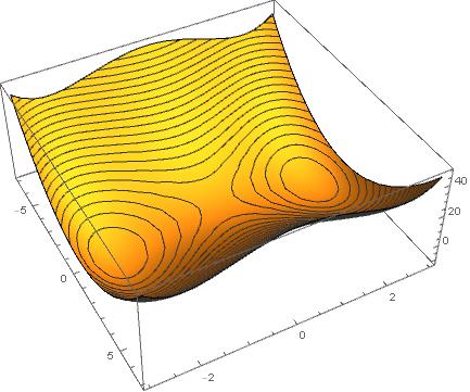
Figure 1: Picture of $H(\psi^{\prime},\psi)$ with $a<0$.

1. $h_{0}=-\frac{p-1}{p+1}(-a)^{\frac{p+1}{p-1}}$. Then

   $$\psi(t)\equiv(-a)^{\frac{1}{p-1}},\quad\forall~{}t\in(-\infty,\infty).$$

2. $h_{0}=0$. Then by a direct computation, for some $\lambda>0$,

   $$\psi(t)=\left(\frac{\left(e^{-(p-1)\sqrt{-a}t}+\lambda^{2}\right)e^{\frac{p-1}{2}\sqrt{-a}t}}{\sqrt{-2a(p+1)\lambda}}\right)^{-\frac{2}{p-1}}=O(1)\cdot e^{-\sqrt{-a}t}.$$

3. $h_{0}\in(-\frac{p-1}{p+1}(-a)^{\frac{p+1}{p-1}},0)$. Then we have a class of periodic solutions which are uniquely determined by $h_{0}.$ See more analysis of $\psi$ in Section 2.1 in [22].

4. $h_{0}>0$. Then the solution must become negative in finite time. Thus there are no positive solutions $\psi$ of (1.8) with $b=0$ and $a<0$ such that $H(\psi^{\prime},\psi)>0$.

$\bullet$ When $b>0,a<0$, by a direct computation,

$$\frac{\mathrm{d}}{\mathrm{d}t}H\left(\psi^{\prime}(t),\psi(t)\right)=-2b\psi^{\prime 2}(t)\leq 0.$$ (A.1)

By a direct computation, (1.8) with $b>0,a<0$ admits two non-negative constant solutions

$$\psi\equiv 0\quad\text{and}\quad\psi\equiv(-a)^{1/(p-1)}.$$

Since $H\left(\psi^{\prime}(t),\psi(t)\right)$ is monotone decreasing and bounded from below, we let

$$h_{-0}:=\lim_{t\rightarrow-\infty}H(\psi^{\prime}(t),\psi(t))\quad\text{and}\quad h_{0}:=\lim_{t\rightarrow+\infty}H(\psi^{\prime}(t),\psi(t)),$$

where $h_{-0}$ may be $+\infty$. We separate into the following cases by $h_{-0}$ and $h_{0}$.

1. $h_{-0}>0$. Then there exists $N$ such that $H\left(\psi^{\prime}(t),\psi(t)\right)>0$ for all $t\in(-\infty,N)$ and $\psi$ vanishes in finite time.

   In fact, if $0<h_{-0}<\infty$, then as shown in Figure 1, $\psi(t)$ is asymptotically periodic and becomes negative in finite time. It remains to rule out $h_{-0}=+\infty$ and $\psi$ always positive case.

   First we claim that for all $t<N$, $\psi^{\prime}(t)<0$ always holds. By contradiction, we assume that for some $t_{0}<N$, $\psi^{\prime}(t_{0})=0,\psi(t_{0})>0$ and $H(0,\psi(t_{0}))>0$. By (1.8), we have $\psi^{\prime\prime}(t_{0})<0$ and thus $\psi^{\prime}(t)<0$ in a left-neighbourhood $(t_{0}-2\epsilon,t_{0})$ of $t_{0}$ for some $\epsilon>0$. As shown in Figure 1, $|\psi^{\prime}|$ has a positive lower bound on $(-\infty,t_{0}-\epsilon]$, contradicting to $\psi>0$.

   However, since $\psi^{\prime}(t)<0$ for all $t<N$, by (1.8) again, there exists $N^{\prime}\ll N$ such that $\psi^{\prime\prime}(t)<-1$ for all $t\in(-\infty,N^{\prime}]$. Thus this makes $\psi^{\prime}(t)<0$ on $(-\infty,N)$ cannot happen.

2. $h_{-0}=0,h_{0}=0$. Then $\psi\equiv 0$.

3. $h_{-0}\leq 0,h_{0}<0$. Then $\psi(t)$ is asymptotically periodic to a positive periodic solution of (1.8) with $b=0$. Thus by (1.8), $\psi^{\prime\prime}(t)$ is bounded. On the other hand, by (A.1), $2b\psi^{\prime 2}(t)$ is integrable on $[1,+\infty)$. Thus (see for instance the proof of (3.19))

   $$\lim_{t\rightarrow+\infty}\psi^{\prime}(t)=0\quad\text{and}\quad\lim_{t\rightarrow+\infty}\psi(t)=\psi(+\infty)$$

   for some constant $\psi(+\infty)$. By (1.8) again, $\psi^{\prime\prime}(t)\rightarrow 0$ as $t\rightarrow+\infty$ and thus $\psi(+\infty)$ is a constant solution of (1.8). Since $h_{0}<0$, the only possible case is

   $$\lim_{t\rightarrow+\infty}\psi(t)=(-a)^{1/(p-1)}.$$

$\bullet$ When $a\geq 0$, notice that

$$\inf_{\mathbb{R}\times\mathbb{R}^{+}}H(\alpha,\beta)=\int_{\mathbb{R}}\left(a\cdot\beta^{2}+\frac{2}{p+1}\beta^{p+1}\right)=0.$$

As shown in Figure 2 and the calculus above, the only possible case when $b=0$ is that $\psi(t)\equiv 0$, otherwise the solution would become negative in finite time. When $b>0$, similar to the discussion in $b>0,a<0$ and $h_{-0}>0$ case, $\psi$ also vanishes in finite time. Thus there are no positive smooth solutions when $a\geq 0$.

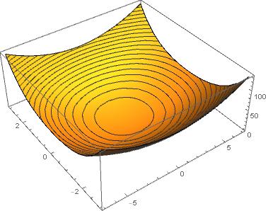
Figure 2: Picture of $H(\psi^{\prime},\psi)$ with $a\geq 0$.

Especially, Jin-Li-Xu [21] proved the following radial symmetry of global solutions.

Theorem A.1.

Let $f(x,t):\mathbb{R}^{n}\backslash\{0\}\times[0,\infty)\rightarrow[0,\infty)$ be a continuous function such that for any $x\neq 0,0<\lambda<|x|,|z|>\lambda$ and $a\leq b,$ there holds

$$\left(\frac{\lambda}{|z|}\right)^{n+2}f\left(x+\frac{\lambda^{2}z}{|z|^{2}},\left(\frac{|z|}{\lambda}\right)^{n-2}a\right)\leq f(x+z,b).$$ (A.2)

If $v\in C^{2}\left(\mathbb{R}^{n}\backslash\{0\}\right)$ is a positive solution of

$$\Delta v+f(x,v)=0\quad\text{in}~{}\mathbb{R}^{n}\setminus\{0\},$$

with $\limsup_{x\rightarrow 0}v(x)=+\infty$. Then $v$ must be radially symmetric about the origin and $v^{\prime}(r)<0$ for all $0<r<\infty$.

By a direct computation, under assumption (1.6), $f(x,t)=\dfrac{c}{|x|^{2}}t+\dfrac{t^{p}}{|x|^{\sigma}}$ satisfies condition (A.2). Thus all positive smooth solutions of (1.3) with (1.6) in $\mathbb{R}^{n}\setminus\{0\}$ must be radially symmetric if $0$ is not a $C^{0}$-removable singularity. By transform (1.2), so are all positive smooth solutions of (1.1) with

$$\limsup_{t\rightarrow+\infty}e^{\frac{n+b-2}{2}t}u(\theta,t)>0.$$

S. Chen & Z. Liu

School of Mathematical Sciences, Beijing Normal University
Laboratory of Mathematics and Complex Systems, Ministry of Education
Beijing 100875, China
Email:
chenshan_lyla@mail.bnu.edu.cn
liuzixiao@mail.bnu.edu.cn

References

- [1] Thierry Aubin. Some nonlinear problems in Riemannian geometry. Springer Monographs in Mathematics. Springer-Verlag, Berlin, 1998.
- [2] Patricio Aviles. On isolated singularities in some nonlinear partial differential equations. Indiana Univ. Math. J., 32(5):773–791, 1983.
- [3] Patricio Aviles. Local behavior of solutions of some elliptic equations. Comm. Math. Phys., 108(2):177–192, 1987.
- [4] Marie-Françoise Bidaut-Veron and Philippe Grillot. Asymptotic behaviour of the solutions of sublinear elliptic equations with a potential. Appl. Anal., 70(3-4):233–258, 1999.
- [5] Marie-Françoise Bidaut-Véron and Laurent Véron. Nonlinear elliptic equations on compact Riemannian manifolds and asymptotics of Emden equations. Invent. Math., 106(3):489–539, 1991.
- [6] Haïm Brézis and Laurent Véron. Removable singularities for some nonlinear elliptic equations. Arch. Rational Mech. Anal., 75(1):1–6, 1980/81.
- [7] Luis A. Caffarelli, Basilis Gidas, and Joel Spruck. Asymptotic symmetry and local behavior of semilinear elliptic equations with critical Sobolev growth. Comm. Pure Appl. Math., 42(3):271–297, 1989.
- [8] Rayssa Caju, João Marcos do Ó, and Almir Silva Santos. Qualitative properties of positive singular solutions to nonlinear elliptic systems with critical exponent. Ann. Inst. H. Poincaré Anal. Non Linéaire, 36(6):1575–1601, 2019.
- [9] Subrahmanyan Chandrasekhar. An introduction to the study of stellar structure. Dover Publications, Inc., New York, N. Y., 1957.
- [10] Chiun-Chuan Chen and Chang-Shou Lin. Local behavior of singular positive solutions of semilinear elliptic equations with Sobolev exponent. Duke Math. J., 78(2):315–334, 1995.
- [11] Chiun-Chuan Chen and Chang-Shou Lin. Estimates of the conformal scalar curvature equation via the method of moving planes. Comm. Pure Appl. Math., 50(10):971–1017, 1997.
- [12] Huyuan Chen and Feng Zhou. Isolated singularities for elliptic equations with Hardy operator and source nonlinearity. Discrete Contin. Dyn. Syst., 38(6):2945–2964, 2018.
- [13] Florica C. Cîrstea. A complete classification of the isolated singularities for nonlinear elliptic equations with inverse square potentials. Mem. Amer. Math. Soc., 227(1068):vi+85, 2014.
- [14] Florica C. Cîrstea and Maria Fărcăşeanu. Sharp existence and classification results for nonlinear elliptic equations in with Hardy potential. arXiv. 2009.00157, 2020.
- [15] Earl A. Coddington and Norman Levinson. Theory of ordinary differential equations. McGraw-Hill Book Company, Inc., New York-Toronto-London, 1955.
- [16] Jean Dolbeault, Maria J. Esteban, and Michael Loss. Rigidity versus symmetry breaking via nonlinear flows on cylinders and Euclidean spaces. Invent. Math., 206(2):397–440, 2016.
- [17] Basilis Gidas and Joel Spruck. Global and local behavior of positive solutions of nonlinear elliptic equations. Comm. Pure Appl. Math., 34(4):525–598, 1981.
- [18] David Gilbarg and Neil S. Trudinger. Elliptic partial differential equations of second order. Classics in Mathematics. Springer-Verlag, Berlin, 2001. Reprint of the 1998 edition.
- [19] Qing Han, Xiaoxiao Li, and Yichao Li. Asymptotic expansions of solutions of the Yamabe equation and the -Yamabe equation near isolated singular points. arXiv. 1909.07466, 2019.
- [20] Zheng-Chao Han, YanYan Li, and Eduardo V. Teixeira. Asymptotic behavior of solutions to the -Yamabe equation near isolated singularities. Invent. Math., 182(3):635–684, 2010.
- [21] Qinian Jin, YanYan Li, and Haoyuan Xu. Symmetry and asymmetry: the method of moving spheres. Adv. Differential Equations, 13(7-8):601–640, 2008.
- [22] Nick Korevaar, Rafe Mazzeo, Frank Pacard, and Richard Schoen. Refined asymptotics for constant scalar curvature metrics with isolated singularities. Invent. Math., 135(2):233–272, 1999.
- [23] Congming Li. Local asymptotic symmetry of singular solutions to nonlinear elliptic equations. Invent. Math., 123(2):221–231, 1996.
- [24] YanYan Li. Conformally invariant fully nonlinear elliptic equations and isolated singularities. J. Funct. Anal., 233(2):380–425, 2006.
- [25] YanYan Li and Lei Zhang. Liouville-type theorems and Harnack-type inequalities for semilinear elliptic equations. J. Anal. Math., 90:27–87, 2003.
- [26] Yimei Li and Jiguang Bao. Local behavior of solutions to fractional Hardy-Hénon equations with isolated singularity. Ann. Mat. Pura Appl. (4), 198(1):41–59, 2019.
- [27] Pierre-Louis Lions. Isolated singularities in semilinear problems. J. Differential Equations, 38(3):441–450, 1980.
- [28] Fernando C. Marques. Isolated singularities of solutions to the Yamabe equation. Calc. Var. Partial Differential Equations, 32(3):349–371, 2008.
- [29] Quoc Hung Phan and Philippe Souplet. Liouville-type theorems and bounds of solutions of Hardy-Hénon equations. J. Differential Equations, 252(3):2544–2562, 2012.
- [30] Peter Poláčik, Pavol Quittner, and Philippe Souplet. Singularity and decay estimates in superlinear problems via Liouville-type theorems. I. Elliptic equations and systems. Duke Math. J., 139(3):555–579, 2007.
- [31] Leon Simon. Asymptotics for a class of nonlinear evolution equations, with applications to geometric problems. Ann. of Math. (2), 118(3):525–571, 1983.
- [32] Laurent Véron. Singularities of solutions of second order quasilinear equations, volume 353 of Pitman Research Notes in Mathematics Series. Longman, Harlow, 1996.
- [33] Jingang Xiong and Lei Zhang. Isolated singularities of solutions to the Yamabe equation in dimension . arXiv. 2006.13279, 2020.