Improve the Robustness and Accuracy of Deep Neural Network with $L_{2,\infty}$ Normalization

Abstract

In this paper, the robustness and accuracy of the deep neural network (DNN) was enhanced by introducing the $L_{2,\infty}$ normalization of the weight matrices of the DNN with Relu as the activation function. It is proved that the $L_{2,\infty}$ normalization leads to large dihedral angles between two adjacent faces of the polyhedron graph of the DNN function and hence smoother DNN functions, which reduces over-fitting. A measure is proposed for the robustness of a classification DNN, which is the average radius of the maximal robust spheres with the sample data as centers. A lower bound for the robustness measure is given in terms of the $L_{2,\infty}$ norm. Finally, an upper bound for the Rademacher complexity of DNN with $L_{2,\infty}$ normalization is given. An algorithm is given to train a DNN with the $L_{2,\infty}$ normalization and experimental results are used to show that the $L_{2,\infty}$ normalization is effective to improve the robustness and accuracy.

Keywords. Deep neural network, $L_{2,\infty}$ normalization, robust measure, over-fitting, smooth DNN, Rademacher complexity.

1 Introduction

The Deep neural network (DNN) [6] has become the most powerful method in machine learning, which was widely used in computer vision [16], natural language processing [14], and many other fields. A DNN is a composition of multi-layer neurons which are affine transformations together with nonlinear activation functions. The DNN has universal power to approximate any continuous function over a bounded domain [7]. Despite of its huge success, the DNN still has spaces for significant improvements in terms of interpretability, robustness, over-fitting, and existence of adversary samples.

In this paper, we will focus on improving the robustness and reducing the over-fitting of DNNs by introducing the $L_{2,\infty}$ normalization of the weigh matrices of the DNN. We assume that the DNN uses Relu as the activation function, which is one of the widely used models of DNNs. We give theoretical analysis of the $L_{2,\infty}$ normalization in three aspects: (1) It is shown that the $L_{2,\infty}$ normalization leads to larger angles between two adjacent faces of the polyhedron graph of the DNN function and hence smooth DNN functions, which reduces the over-fitting. (2) A measure of robustness for DNNs is defined and a lower bound for the robustness measure is given in terms of the $L_{2,\infty}$ norm. (3) An upper bound for the Rademacher complexity of the DNN in terms of the $L_{2,\infty}$ norm is given. Finally, an algorithm is given to train a DNN with $L_{2,\infty}$ normalization and experimental results are used to show that the $L_{2,\infty}$ normalization is effective to enhance the robustness and accuracy. In the following, we give a brief introduction to the three aspects of theoretical analysis given in this paper and the related work.

When the complexity of the DNN surpasses the complexity of the target function, it may happen that the gap between the DNN and the actual function in the region outside the training data becomes larger along with the training, which is called over-fitting. An over-fitting DNN fits the training data nicely but has low accuracy at the validation set. A simple and effective way to reduce over-fitting is early termination [2, Sec.7.7]. An important reason of over-fitting is that the DNN has too many parameters and an effective method to tackle this problem is the dropout method [15, 17, 11]. $L_{1}$ and $L_{2}$ regulations are also used to reduce the over-fitting [2, Sec.7.1]. The batch normalization is a recently proposed and important method to reduce over-fitting [5].

In this paper, we propose a new approach to alleviate the over-fitting problem. Intuitively, one of the reasons for over-fitting is that the DNN function has too much local fluctuations, and hence to make the DNN function smoother can reduce over-fitting. When the activation function is Relu, the DNN could be considered as a real valued function and its graph is a polyhedron. We prove that the dihedral angle between two adjacent faces of the polyhedron graph of a DNN can be nicely bounded by the $L_{2,\infty}$ norm, and hence the $L_{2,\infty}$ normalization leads to smoother DNN functions and less over-fitting. In [10], the number of faces of the polyhedron graph is estimated and is treated as a measure for the representation power of the DNN. In this paper, we try to control the refined geometric structure of the graph polyhedron to reduce the over-fitting and to increase the robustness.

Robustness is a key desired feature for DNNs. Roughly speaking, a network is robustness if it has high accuracy at the input with little noise and does not have a devastating hit when facing big noise. It is clear that a more robust network is less possible to have adversary examples [9, 3]. Adding noises to the training data is an effective way to increase the robustness [2, Sec.7.5]. The $L_{1}$ regulation and $L_{1,\infty}$ normalization are used to increase the robustness of DNNs [18]. Knowledge distilling is also used to enhance robustness and defend adversarial examples [3]. In [8], linear programming is used to check whether a DNN is robust over a given region. In [1], three methods were given to test the robustness of DNNs by experimental results.

In the above work, the robustness of the DNNs was usually demonstrated by experimental results and there exists no measure for the robustness. In this paper, we give a preliminary try on this direction by defining a measure for the robustness of classification DNNs, which is the average volume or radius of the maximal robust spheres with the training sample points as centers. We give a lower bound for this measure of robustness in terms of the $L_{2,\infty}$ norm, and show that the lower bound is reasonably good for simple networks.

The Rademacher complexity is used to measure the richness of a class of real-valued functions. When there exist no bias vectors, the Rademacher complexity of DNNs with $L_{p,q}$ normalization was estimated in [13]. In this paper, we give an upper bound for the Rademacher complexity of general DNNs in terms of the $L_{2,\infty}$ norm.

The rest of this paper is organized as follows. In Section 2, the $L_{2,\infty}$ normalization of DNNs is defined. In Section 3, it is shown that the $L_{2,\infty}$ normalization will lead to smoother graphs for the DNN. In Section 4, a measure of robustness is defined and a lower bound for the measure is given. In Section 5, an upper bound for the Rademacher complexity for DNNs with $L_{2,\infty}$ normalization is given. In Section 6, an algorithm and experimental results are given.

2 $L_{2,\infty}$ normalization of DNN

In this section, we present the $L_{2,\infty}$ normalization of DNNs.

2.1 The standard DNN

A feed-forward deep neural network (DNN) can be represented by

$$\begin{array}[]{ll}x_{l}=f_{l}(W_{l}x_{l-1}+b_{l})\in{\mathbb{R}}^{n_{l}},l=1,2,\ldots,L,\\ f_{l}:{\mathbb{R}}^{n_{l}}\rightarrow{\mathbb{R}}^{n_{l}},W_{l}\in{\mathbb{R}}^{n_{l}\times n_{l-1}},b_{l}\in{\mathbb{R}}^{n_{l}}\end{array}$$ (1)

where $x_{0}\in{\mathbb{R}}^{n_{0}}$ is the input, $x_{L}\in{\mathbb{R}}^{n_{L}}$ is the output, and $x_{l}=f^{l}(W_{l}x_{l-1}+b_{l}),l=1,2,\ldots,L-1$ is the $l$-th hidden layer. $W_{l}$ is called the weight matrix and $b_{l}$ the bias vector. $f_{l}$ is a non-linear activation function. In this paper, we assume that $f^{l}$ is Relu when $l\in\{1,2,\dots,L-1\}$ and $f_{L}=I_{n_{L}}$ unless mentioned otherwise.

For simplicity, we assume that the input data are from $[0,1]^{n_{0}}$ or ${\mathbb{R}}^{n_{0}}$. We denote this DNN by

$${\mathcal{F}}:{\mathbb{R}}^{n_{0}}(\hbox{\rm{or}}\ [0,1]^{n_{0}})\rightarrow{\mathbb{R}}^{n_{L}}\hbox{ with parameters }\Theta_{\mathcal{F}}=\{W_{l},b_{l}\,|\,l=1,\ldots,L\}.$$ (2)

For instance, a sample in MINST is a $28\cdot 28=784$ dimensional vector in $[0,1]^{784}$.

Given a training data set $S=\{(x_{i},y_{i})\in{\mathbb{R}}^{n_{0}}\times{\mathbb{R}}^{n_{L}}\,|\,i=1,\ldots,K\}$, we have the loss function ${\hbox{\rm{Loss}}}=\frac{1}{K}\sum^{K}_{i=1}{L({\mathcal{F}}(x_{i}),y_{i})}$, where $L$ could be the cross entropy or other functions. To train the DNN, we use gradient descent to update $\Theta_{\mathcal{F}}$ in order to make Loss as small as possible. In the end, we achieve the minimum point $\Theta_{0}$ such that $\bigtriangledown{\mathcal{F}}(\Theta_{0})\approx 0$, and obtain the trained DNN ${\mathcal{F}}$ with the parameters $\Theta_{0}$.

2.2 The $L_{2,\infty}$ normalization

The $L_{2,\infty}$ norm of a matrix $M$ is the maximum of the $L_{2}$ norm of the rows of M:

$$||M||_{2,\infty}=\max_{w}\{||w||_{2}\,:\,w\,\hbox{\rm is a row of }M\}.$$

Lemma 2.1.

If the $L_{2,\infty}$ norm of two matrices $A,B\in{\mathbb{R}}^{n\times n}$ are both smaller than $c$, then the $L_{2,\infty}$ norm of $AB$ is smaller than $\sqrt{n}*c^{2}$.

Proof.

Let $a_{i,j}$ and $b_{i,j}$ be the entries of $A$ and $B$, respectively. The first row of $C=AB$ is $(\sum^{n}_{i=1}a_{1,i}*b_{i,j})^{n}_{j=1}$. Since $(\sum^{n}_{i=1}a_{1,i}*b_{i,j})^{2}\leq(\sum^{n}_{i=1}(a_{1,i})^{2})(\sum^{n}_{i=1}(b_{i,j})^{2})$, the square of the $L_{2}$ norm of the first row of $C$ is smaller than

$$\sum^{n}_{j=1}(\sum^{n}_{i=1}a_{1,i}*b_{i,j})^{2}\leq\sum^{n}_{j=1}(\sum^{n}_{i=1}(a_{1,i})^{2})(\sum^{n}_{i=1}(b_{i,j})^{2})=(\sum^{n}_{i=1}(a_{1,i})^{2})*(\sum^{n}_{i,j=1}(b_{i,j})^{2})\leq c^{2}\times nc^{2}.$$

So the $L_{2,\infty}$ norm of $AB$ is smaller than $\sqrt{n}*c^{2}$. ∎

We now introduce a new constraint to the DNN ${\mathcal{F}}$.

Definition 2.1.

Let ${\mathcal{F}}$ be the DNN defined in (2) and $c\in{\mathbb{R}}_{>0}$. The $||L||_{2,\infty}$ normalization of ${\mathcal{F}}$ is defined to be $||W_{l}||_{2,\infty}\leqslant c,l=1,\ldots,L$.

Note that the bias vectors are not considered in this constraint.

3 Geometric meaning of $L_{2,\infty}$ normalization

In this section, we give the geometric meaning of the $L_{2,\infty}$ normalization and show that it can be used to reduce the over-fitting of DNNs.

3.1 Graph of DNN with Relu activation

We assume that ${\mathcal{F}}$ is a standard DNN defined in (2) and $n_{L}=1$. Since $n_{L}=1$, the DNN is a real valued function ${\mathcal{F}}:[0,1]^{n_{0}}\rightarrow{\mathbb{R}}$. Since the activation function of ${\mathcal{F}}$ is Relu, ${\mathcal{F}}$ is a piecewise linear function. Let $n_{\mathcal{F}}=n_{0}+1$. The graph of ${\mathcal{F}}$ is denoted by ${\mathcal{F}}_{g}$, which is a polyhedron in ${\mathbb{R}}^{n_{\mathcal{F}}}$.

A linear region of ${\mathcal{F}}$ is a maximal connected open subset of the input space $[0,1]^{n_{0}}$, on which F is linear [10]. Over a linear region, there exists a $W\in{\mathbb{R}}^{n_{0}}$ and $b\in{\mathbb{R}}$ such that ${\mathcal{F}}(x)=W^{\tau}x+b$. Thus, $F_{g}$ is a part of a hyperplane on every linear region, and we call this part of hyperplane a face of ${\mathcal{F}}_{g}$.

Lemma 3.1.

The linear regions of ${\mathcal{F}}$ satisfy the following properties [10].

(1) A linear region $R$ is an $n_{0}$-dimensional polyhedron defined by a set of linear inequalities $C_{i}^{\tau}x+b_{i}>0,i=1,\ldots,L_{R}$, where $C_{i}\in{\mathbb{R}}^{n_{0}}$ and $b_{i}\in{\mathbb{R}}$.

(2) The input space of ${\mathcal{F}}$ is the union of the closures of the linear regions of ${\mathcal{F}}$.

Definition 3.1.

Two faces $A$ and $B$ of ${\mathcal{F}}_{g}$ are said to be adjacent if $\overline{R}_{A}\cap\overline{R}_{B}$ is an $(n_{0}-1)$-dimensional polyhedron, where $\overline{R}_{A}$ and $\overline{R}_{B}$ are the closures of $R_{A}$ and $R_{B}$, respectively.

When training the network ${\mathcal{F}}$, we randomly choose initial values and do gradient descent to make the loss function as small as possible. It is almost impossible to make ${\hbox{\rm{Loss}}}=0$ and we may assume that the training terminates at a random point in the neighborhood of one of the minimal points of the loss function. Therefore, the following assumption is valid for almost trained DNNs.

Assumption 3.1.

The trained parameters of ${\mathcal{F}}$ are random values near a minimum point of the loss function.

Lemma 3.2 ([4]).

Let $x_{0}$ be a randomly chosen point in $[0,1]^{n}$ and $H(x)$ a polynomial in $n$ variables. Then the probability for $H(x_{0})=0$ is zero.

Now we will give two lemmas under the Assumption 3.1. Due to Lemma 3.2, the results proved under Assumption 3.1 are correct with probability one. We will not mention this explicitly in the descriptions of the lemmas and theorems below.

Lemma 3.3.

Under Assumption 3.1, one row of the weight matrix $W^{l}$ is not the multiple of another row of $W^{l}$.

Proof.

Let $W_{l,i,j}$ be the element of $W_{l}$ at the $i$-th row and $j$-th column. If the $i_{1}$-th row of $W_{l}$ is a multiple of the $i_{2}$-th row of $W_{l}$, then the parameters of these two rows must satisfy $W_{l,i_{1},j}\cdot W_{l,i_{1},k}=W_{l,i_{1},k}\cdot W_{l,i_{1},j}$ for all $j\neq k$. By Lemma 3.2, probability for this to happen is zero. ∎

The following result shows that two adjacent faces are caused by a single Relu function.

Lemma 3.4.

Let $A,B$ be two adjacent faces of ${\mathcal{F}}_{g}$ and $R_{A},R_{B}$ their linear regions, respectively. Under Assumption 3.1, there exists a unique Relu function $f_{c}$ of ${\mathcal{F}}$ such that (1) all Relu functions of ${\mathcal{F}}$ except $f_{c}$ are either $0$ or positive over $R_{A}\cup R_{B}$; (2) $f_{c}=0$ over $A$ and $f_{c}>0$ over $B$.

Proof.

Assume the contrary: ${\mathcal{F}}$ has two Relu functions satisfying (1) and (2). We assume they are the $l_{1}$-th and $l_{2}$-th layers and $l_{1}<l_{2}$. Then we can calculate $F(x_{0})$ for $x_{0}\in R_{A}\cup R_{B}$ by:

$$x_{l_{1}} = W_{l_{1}}x_{0}+b_{l_{1}}$$

$$x_{l_{1}+1} = W_{l_{1}+1}x_{l_{1}}+b_{l_{1}+1}+{\hbox{\rm{Relu}}}(h_{1}x_{l_{1}}+d_{1})$$

$$x_{l_{2}} = W_{l_{2}}x_{l_{1}+1}+b_{l_{2}}$$

$$x_{l_{2}+1} = W_{l_{2}+1}x_{l_{2}}+b_{l_{2}+1}+{\hbox{\rm{Relu}}}(h_{2}x_{l_{2}}+d_{2})$$

$$F(x_{0}) = Wx_{l_{2}+1}+d$$

where $W_{l_{j}}$, $W_{l_{j}+1}$, $W$ are weight matrices and $b_{l_{j}}$, $b_{l_{j}+1}$, $d$ bias vectors. In particular, $h_{j}$ is a matrix whose elements are $0$ except one row and $d_{i}$ is a vector whose elements are zero except one component, because the activity function changes sign when going from $R_{A}$ to $R_{B}$.

Assume the common boundary of $R_{A}$ and $R_{B}$ has the normal vector $K$ and a point $x_{k}$ is on this boundary. Denote $f_{c}(M)$ to be the first nonzero row of the matrix $M$. Then, we have the following relations.

$$h_{1}W_{l_{1}}x_{k}+h_{1}b_{l_{1}}+d_{1}=0$$

$$f_{c}(h_{1}W_{l_{1}})=K$$

$$h_{2}(W_{l_{2}}(W_{l_{1}+1}(W_{l_{1}}x_{k}+b_{l_{1}})+b_{l_{1}+1})+b_{l_{2}})+d_{2}=0$$

$$f_{c}(h_{2}W_{l_{2}}W_{l_{1}+1}W_{l_{1}})=K.$$

Eliminating $x_{k}$ and $K$, we have

$$f_{c}(h_{2}W_{l_{2}}W_{l_{1}+1}W_{l_{1}})=f_{c}(h_{1}W_{l_{1}})$$

$$f_{c}(h_{1}b_{l_{1}}+d_{1})=f_{c}(h_{2}W_{l_{2}}W_{l_{1}+1}b_{l_{1}}+h_{2}W_{l_{2}}b_{l_{1}+1}+h_{2}b_{l_{2}}+d_{2}).$$

By Lemma 3.2, under Assumption 3.1, ${\mathcal{F}}$ cannot satisfy these equations with probability $1$. The lemma is proved. ∎

3.2 $L_{2,\infty}$ normalization and dihedral angle between two adjacent faces of ${\mathcal{F}}_{g}$

If the dihedral angle between two adjacent faces of ${\mathcal{F}}_{g}$ is large, then ${\mathcal{F}}_{g}$ is a smooth polyhedron. The dihedral angle between two hyperplanes $\sum^{n}_{i=1}a_{k,i}x_{i}+b_{k}=0,k=1,2$ is

$$\arccos\frac{\sum^{n}_{i=1}a_{1,i}a_{2,i}}{\sqrt{\sum_{i=1}^{n}(a_{1,i})^{2}}\sqrt{\sum_{i=1}^{n}(a_{2,i})^{2}}}.$$

If the hyperplanes are directional, then the dihedral angle will be $\arccos\frac{\sum^{n}_{i=1}a_{1,i}a_{2,i}}{\sqrt{\sum_{i=1}^{n}(a_{1,i})^{2}}\sqrt{\sum_{i=1}^{n}(a_{2,i})^{2}}}$ or $\pi-\arccos\frac{\sum^{n}_{i=1}a_{1,i}a_{2,i}}{\sqrt{\sum_{i=1}^{n}(a_{1,i})^{2}}\sqrt{\sum_{i=1}^{n}(a_{2,i})^{2}}}$, assuming $\arccos(x)\in[0,\pi]$.

We first consider a simple DNN with one hidden layer

$${\mathcal{H}}:{\mathbb{R}}^{n}\rightarrow{\mathbb{R}},\hbox{ where }{\mathcal{H}}(x)=L\cdot{\hbox{\rm{Relu}}}(Wx+b)+d.$$

Let $W=[w_{1}^{\tau},w_{2}^{\tau},\ldots,w_{m}^{\tau}]^{\tau}\in{\mathbb{R}}^{m\times n}$, $L^{\tau}=[l_{1},l_{2},\ldots,l_{m}]^{\tau}\in{\mathbb{R}}^{m}$, and $b^{\tau}=(b_{1},b_{2},\ldots,b_{m})^{\tau}\in{\mathbb{R}}^{m}$. Then

$${\mathcal{H}}(x)=\sum_{i=1}^{m}l_{i}\ {\hbox{\rm{Relu}}}(w_{i}x+b_{i})+d.$$ (3)

We can give an estimation of the dihedral angle between two adjacent faces of ${\mathcal{H}}_{g}$.

Lemma 3.5.

If the $L_{2,\infty}$ norm of the weight matrices of ${\mathcal{H}}$ is smaller than $c$, then under Assumption 3.1, the dihedral angle between two adjacent faces of ${\mathcal{H}}_{g}$ is bigger than $\pi-\arccos\frac{1}{\sqrt{1+c^{2}}}$ or $\pi-\arccos\frac{4-c^{2}}{4+c^{2}}$.

Proof.

Let $x\in{\mathbb{R}}^{n}$ be the input and $y\in{\mathbb{R}}$ the output. From (3), the face of the polyhedron ${\mathcal{H}}_{g}$ has the expression -y+$\sum_{i=1}^{m}l_{i}m_{i}(w_{i}x+b_{i})+d=0$, where $m_{i}$ is $1$ or $0$ depending on whether $w_{i}x+b_{i}$ is bigger than $0$ or not. For two adjacent faces $A_{f}$ and $B_{f}$, by Lemma 3.4, there exists a unique $m_{i}$, which is respectively $0$ and $1$ over $A_{R}$ and $B_{R}$ (the linear regions of $A_{f}$ and $B_{f}$), and $m_{j}$ has fixed sign over these two linear regions for $j\neq i$. So the two adjacent faces are defined by

$$y=W_{a}x+b_{a}\hbox{ and }y=W_{a}x+l_{i}w_{i}x+b_{a}+l_{i}b_{i}.$$

Since $W_{a}=\sum_{j=1}^{m}l_{j}m_{j}w_{j}$, the normal vectors of the two adjacent faces are $\{-1,W_{a}\}$ and $\{-1,W_{a}+l_{i}w_{i}\}$, respectively. We denote

$$D=\arccos\frac{1+||W_{a}||^{2}_{2}+l_{i}W_{a}\cdot w_{i}}{\sqrt{1+||W_{a}+l_{i}w_{i}||^{2}_{2}}\sqrt{1+||W_{a}||^{2}_{2}}}=\arccos\frac{1+||W_{a}||^{2}_{2}+l_{i}W_{a}\cdot w_{i}}{\sqrt{1+||W_{a}||_{2}^{2}+||l_{i}w_{i}||^{2}_{2}+2l_{i}W_{a}\cdot w_{i}}\sqrt{1+||W_{a}||^{2}_{2}}},$$

where $\cdot$ is the inner product. Since the first components of the normal vactors are $-1$, the dihedral angle between the two faces are $\pi-D$. It suffices to prove $D\leq\arccos\frac{1}{\sqrt{1+c^{2}}}$ or $D\leq\arccos\frac{4-c^{2}}{4+c^{2}}$.

Define a univariate function: $G(x)=\frac{1+A+x}{\sqrt{1+A+B+2x}}$, where $A>0$, $B>0$ and $\sqrt{AB}\geq x\geq-\sqrt{AB}$. Then $G^{\prime}(x)=\frac{B+x}{(1+A+B+2x)^{1.5}}$. That is, the minimum point of G(x) is $-\sqrt{AB}$ or $-B$. We will use this function to analyse the dihedral angle. We divide the discussion into two cases.

Case 1: assume $||W_{a}||^{2}_{2}\geq||l_{i}w_{i}||^{2}_{2}$. Let $||W_{a}||^{2}_{2}=A$, $||l_{i}w_{i}||^{2}_{2}=B$ and use the property for function $G(x)$. When $||l_{i}w_{i}||^{2}_{2}=-2l_{i}W_{a}\times w_{i}$, the angle achieves the maximal value:

$$D\leq\arccos\frac{1+||W_{a}||^{2}_{2}-||l_{i}w_{i}||^{2}_{2}}{\sqrt{1+||W_{a}||_{2}^{2}-||l_{i}w_{i}||^{2}_{2}}\sqrt{1+||W_{a}||^{2}_{2}}}=\arccos\frac{\sqrt{1+||W_{a}||^{2}_{2}-||l_{i}w_{i}||^{2}_{2}}}{\sqrt{1+||W_{a}||^{2}_{2}}}$$

We have $||l_{i}w_{i}||^{2}_{2}\leq c^{2}$ due to the $L_{2,\infty}$ normalization and the assumption $||W_{a}||^{2}_{2}\geq||l_{i}w_{i}||^{2}_{2}$. Then we have

$$\arccos\frac{\sqrt{1+||W_{a}||^{2}_{2}-||l_{i}w_{i}||^{2}_{2}}}{\sqrt{1+||W_{a}||^{2}_{2}}}\leq\arccos\frac{\sqrt{1+||l_{i}w_{i}||^{2}_{2}-||l_{i}w_{i}||^{2}}}{\sqrt{1+||l_{i}w_{i}||^{2}_{2}}}\leq\arccos\frac{1}{\sqrt{1+c^{2}}}.$$

This proves the first bound in the lemma.

Case 2: assume $||W_{a}||^{2}_{2}<||l_{i}w_{i}||^{2}_{2}$. By the property of function $G(x)$, when $l_{i}W_{a}\cdot w_{i}=-||W_{a}||_{2}||l_{i}w_{i}||_{2}$, the angle is the biggest:

$$D\leq\arccos\frac{1+||W_{a}||^{2}_{2}-||W_{a}||_{2}||l_{i}w_{i}||_{2}}{\sqrt{1+||W_{a}||_{2}^{2}+||l_{i}w_{i}||^{2}_{2}-2||W_{a}||_{2}||l_{i}w_{i}||_{2}}\sqrt{1+||W_{a}||^{2}_{2}}}.$$

Denote $K=||l_{i}w_{i}||_{2}-||W_{a}||_{2}$ and $T=||W_{a}||_{2}$. Then it becomes

$$\arccos\frac{1-TK}{\sqrt{1+K^{2}}\sqrt{1+T^{2}}}.$$

Since $0\leq T\leq T+K\leq c$, we have

$$\arccos\frac{1-TK}{\sqrt{1+K^{2}}\sqrt{1+T^{2}}}\leq\arccos\frac{4-c^{2}}{4+c^{2}}.$$

This is because $\frac{1-TK}{\sqrt{1+K^{2}}\sqrt{1+T^{2}}}\geq\frac{4-c^{2}}{4+c^{2}}$, which will be proved below. Taking square and simplifying, it becomes

$$(\frac{4+c^{2}}{4-c^{2}})^{2}(TK-1)^{2}\geq 1+T^{2}+K^{2}+T^{2}K^{2}.$$

We know $c^{2}\geq T^{2}+K^{2}+2TK$ and $(TK-1)^{2}\geq(1-c^{2}/4)^{2}$. Then we have

$$1+T^{2}+K^{2}+T^{2}K^{2}\leq c^{2}+(TK-1)^{2}\leq(\frac{4+c^{2}}{4-c^{2}})^{2}(TK-1)^{2}.$$

We prove the second bound in the lemma. ∎

Remark 3.1.

When $c$ is small, $\arccos\frac{1}{\sqrt{1+c^{2}}}$ and $\arccos\frac{4-c^{2}}{4+c^{2}}$ is approximately $0$ and hence the dihedral between two adjacent faces of ${\mathcal{H}}_{g}$ will be large, as shown by Figures 2 and 2, which show that the $L_{2,\infty}$ normalization makes the DNN function smooth.

Figure 1: $\pi-\arccos(\frac{1}{\sqrt{1+x^{2}}})$

Figure 2: $\pi-\arccos(\frac{4-x^{2}}{4+x^{2}})$

For the general DNN, we can obtain similar results.

Theorem 3.1.

Let ${\mathcal{F}}$ be a DNN defined in (2) and $n_{j}=n$ for all $j\in\{1,2,\dots,L-1\}$. If the $L_{2,\infty}$ norm of all weight matrices of ${\mathcal{F}}$ is smaller than $c$, then the dihedral angle between two adjacent faces of ${\mathcal{F}}_{g}$ is bigger than

$$\pi-\arccos(\frac{1}{\sqrt{1+c^{L}n^{\frac{L-2}{2}}}})\hbox{ {\rm{or}} }\pi-\arccos(\frac{4-c^{L}n^{\frac{L-2}{2}}}{4+c^{L}n^{\frac{L-2}{2}}}).$$

Proof.

Let $A,B$ be two adjacent faces of ${\mathcal{F}}_{g}$, and $R_{A}$, $R_{B}$ their linear regions, respectively. We assume that ${\mathcal{F}}$ satisfies Assumption 3.1. By Lemma 3.4, there exists a unique activation function which changes its sign over $R_{A}\cup R_{B}$. We assume that this happens on the $k$-th layer where $1\leq k\leq L-1$. Then the activation function on the first $k-1$ layer and the last $k+1$ layers have the same sign on $R_{A}\cup R_{B}$, that is,

$$x_{k-1}=U_{k,1}x_{0}+e_{k,1},\ x_{k}={\hbox{\rm{Relu}}}(W_{k}x_{k-1}+b^{k}),\ {\mathcal{F}}(x_{0})=U_{k,2}x_{k}+e_{k,2}$$ (4)

for all $x_{0}$ in $R_{A}\cup R_{B}$, where $U_{k,1}\in{\mathbb{R}}^{n_{k-1}\times n_{0}}$, $e_{k,1}\in{\mathbb{R}}^{n_{k-1}}$, $U_{k,2}\in{\mathbb{R}}^{1\times n_{k}}$, $e_{k,2}\in{\mathbb{R}}$. Then we have

$$x_{k}={\hbox{\rm{Relu}}}(W_{k}x_{k-1}+b^{k})={\hbox{\rm{Relu}}}(W_{k}(U_{k,1}x_{0}+e_{k,1})+b^{k})={\hbox{\rm{Relu}}}(U\cdot x_{0}+\hat{b}^{k}),$$ (5)

where $U=W_{k}U_{k,1}$ and $\widehat{b}_{k}=b_{k}+W_{k}e_{k,1}$. Let $k$ be defined in (4). We first treat ${\mathcal{F}}$ as a one-hidden-layer network whose input is $x_{0}$, and can be computed as in (5). Then because of Lemma 2.1, we know the $L_{2,\infty}$ norm of $U_{k,2}$ is smaller than $c^{L-k}n^{\frac{L-k-1}{2}}$, and the $L_{2,\infty}$ norm of $U$ is smaller than $c^{k}n^{\frac{k-1}{2}}$. Then, the theorem can be proved similarly to Lemma 3.5. ∎

Corollary 3.1.

If $U_{k,1}$ in (4) is the multiple of an orthogonal matrix, then the dihedral angle between $A$ and $B$ is bigger than

$$\pi-\arccos\frac{1}{\sqrt{1+c^{L-k+1}\times n^{\frac{L-k-1}{2}}}}\hbox{ {\rm{or}} }\pi-\arccos\frac{4-c^{L-k+1}\times n^{\frac{L-k-1}{2}}}{4+c^{L-k+1}\times n^{\frac{L-k-1}{2}}}.$$

Proof.

Let $k$ be defined in (4). We first treat ${\mathcal{F}}$ as a one-hidden-layer network whose input is $x_{k-1}$, and can be computed as in (4). From Lemma 2.1, the $L_{2,\infty}$ norm of $U_{k,2}$ is smaller than $c^{L-k}n^{\frac{L-k-1}{2}}$ and the $L_{2,\infty}$ norm of $W_{k}$ is smaller than $c$. On the other hand, when $U_{k,1}$ in (4) is the multiple of an orthogonal matrix, it does not change the angle. Finally, the result can be proved similarly to Lemma 3.5. ∎

4 $L_{2,\infty}$ normalization and robustness of DNN

In this section, we show that the $L_{2,\infty}$ normalization leads to more robust DNNs by proving a lower bound of the robust region of the DNN.

We assume that ${\mathcal{F}}$ is a classification DNN, that is, its output values $\widehat{{\mathcal{F}}}$ are discrete. To simplify the discussion, we assume that $n_{L}=2$ and if the first coordinate of ${\mathcal{F}}(x)$ is bigger than the second one, then $\widehat{{\mathcal{F}}}(x)=0$ and $1$ otherwise.

Let $\theta$ be a continuous open set in ${\mathbb{R}}^{n_{0}}$. ${\mathcal{F}}$ is said to be robust over $\theta$ if $\widehat{{\mathcal{F}}}$ gives the same label for all $x\in\theta$. We also say that $\theta$ is a robust region of ${\mathcal{F}}$.

Denote $B_{x,r}$ to be the spherical ball with center $x$ and radius $r$. Since ${\mathcal{F}}$ is piecewise linear and continuous, for almost all input $x\in{\mathbb{R}}^{n_{0}}$, $B_{x,\epsilon}$ is a robust region of ${\mathcal{F}}$ if $\epsilon$ is small enough. For any $x\in{\mathbb{R}}^{n_{0}}$, let $r_{x}$ be the maximum value such that $B_{x,r_{x}}$ is a robust region of ${\mathcal{F}}$. Then the volume of $B_{x,r_{x}}$ is

$$A_{x}=C_{n_{0}}r^{n_{0}}_{x}$$

where $C_{n}=\frac{\pi^{n}}{\Gamma(n/2-1)}$ and $\Gamma(x)=\int_{0}^{\infty}t^{x-1}e^{-t}dt$ for all $n\in Z_{+}$. Note that $C_{n}$ just depends on $n$. We now define a measure for the robustness of ${\mathcal{F}}$.

Definition 4.1.

Let ${\mathcal{S}}$ be the training set of network ${\mathcal{F}}$, $|{\mathcal{S}}|=m$, and ${\mathcal{S}}=\{(x_{i},y_{i})\,|\,i=1,\ldots,m\}$. We set $G_{{\mathcal{F}},{\mathcal{S}}}=\{i|\widehat{F}(x_{i})=L(x_{i})\}$, where $L(x_{i})$ is the label of $x_{i}$. Then the robust volume and the robust radius of ${\mathcal{F}}$ are defined respectively as

$$V_{{\mathcal{F}},{\mathcal{S}}}=\frac{\sum_{i\in G_{{\mathcal{F}},{\mathcal{S}}}}A_{x_{i}}}{m}\,\,\hbox{\rm and }\,r_{{\mathcal{F}},{\mathcal{S}}}=\frac{\sum_{i\in G_{{\mathcal{F}},{\mathcal{S}}}}r_{x_{i}}}{m}.$$

Since ${\mathcal{F}}$ is a classification DNN, most of the training data should be in $G_{{\mathcal{F}},{\mathcal{S}}}$, so the above definition measures for the robustness of the DNN in certain sense. $V_{{\mathcal{F}},{\mathcal{S}}}$ is the average volume of maximal robust spheres with the sample points as centers and $r_{{\mathcal{F}},{\mathcal{S}}}$ is the average radius of such spheres. We will show that the $L_{2,\infty}$ normalization will lead to a lower bound for $V_{{\mathcal{F}},{\mathcal{S}}}$ and $r_{{\mathcal{F}},{\mathcal{S}}}$.

We first consider a simple network ${\mathcal{H}}:{\mathbb{R}}^{n}\rightarrow{\mathbb{R}}^{2}$, which has one hidden layer with dimension $n$, with activation function Relu, and output $0$ and $1$. Then

$${\mathcal{H}}(x)=L\cdot{\hbox{\rm{Relu}}}(Wx+b)+d$$ (6)

where ${W,L}$ are the weight matrices and ${b,d}$ are the bias vectors. If the first coordinate ${\mathcal{H}}(x)$ is bigger than the second one, the DNN outputs $\widehat{{\mathcal{H}}}(x)=0$ and $1$ otherwise.

Lemma 4.1.

For the DNN ${\mathcal{H}}$ defined in (6), if the $L_{2,\infty}$ norm of the weight matrices of ${\mathcal{H}}$ is smaller than $c$, then $||{\mathcal{H}}(x+\alpha)-{\mathcal{H}}(x)||_{\infty}\leq c^{2}||\alpha||_{2}$ for $x,\alpha\in{\mathbb{R}}^{n}$.

Proof.

We have ${\mathcal{H}}(x)=L\cdot{\hbox{\rm{Relu}}}(Wx+b)+d$ and ${\mathcal{H}}(x+\alpha)=L\cdot{\hbox{\rm{Relu}}}(Wx+W\alpha+b)+d$. Then $|{\mathcal{H}}(x+\alpha)-{\mathcal{H}}(x)|\leq|L\cdot(W\alpha)|$. Because of the $L_{2,\infty}$ norm constraint, we obtain $||{\mathcal{H}}(x+\alpha)-{\mathcal{H}}(x)||_{\infty}\leq c^{2}||\alpha||_{2}$. ∎

We assume that ${\mathcal{S}}$ is the training set of ${\mathcal{H}}$, and the loss function is square norm or crossentropy (when we choose crossentropy, the output layer uses activation function Softmax). Then we have the result below.

Lemma 4.2.

Assume that the loss function is the square norm, the value of the loss function on ${\mathcal{S}}$ is smaller than $\epsilon$, the accuracy of ${\mathcal{H}}$ on the training set is bigger than $\gamma$, and $\gamma>2\epsilon$. If the $L_{2,\infty}$ norm of the weight matrices is smaller than $c$, then we have

$$V_{{\mathcal{H}},{\mathcal{S}}}\geq C_{n}\frac{(\gamma-\sqrt{2\epsilon\gamma})^{n}}{2^{n}\cdot c^{2n}\cdot\gamma^{n-1}}\,\hbox{\rm and }r_{{\mathcal{H}}}\geq\frac{\gamma-\sqrt{2\epsilon\gamma}}{2c^{2}}.$$

Proof.

Let the training set be ${\mathcal{S}}=\{(x_{i},y_{i})\,|\,i=1,\ldots,m\}$, where $y_{i}=[1,0]$ when the label of $x_{i}$ is $0$, and $y_{i}=[0,1]$ when the label of $x_{i}$ is $1$. Since the loss function is square norm, we have ${\hbox{\rm{Loss}}}=\frac{1}{m}\sum^{m}_{i=1}[({{\mathcal{H}}}_{0}(x_{i})-y_{i,0})^{2}+({{\mathcal{H}}}_{1}(x_{i})-y_{i,1})^{2}]$, where $y_{i,0}$ ($y_{i,1}$) is the first (second) component of $y_{i}$. We can also write it as ${\hbox{\rm{Loss}}}=\frac{1}{m}\sum_{i=1}^{m}[(1-{\mathcal{H}}_{c_{i}}({x_{i}}))^{2}+({\mathcal{H}}_{f_{i}}(x_{i}))^{2}]$, where $c_{i}$ is the label of $x_{i}$ and $f_{i}=1-c_{i}$.

Since the value of loss function is smaller than $\epsilon$, we have

$$\sum_{i\in G_{{\mathcal{H}},{\mathcal{S}}}}[(1-{\mathcal{H}}_{c_{i}}({x_{i}}))^{2}+({\mathcal{H}}_{f_{i}}(x_{i}))^{2}]\leq\sum_{i=1}^{m}[(1-{\mathcal{H}}_{c_{i}}({x_{i}}))^{2}+({\mathcal{H}}_{f_{i}}(x_{i}))^{2}]\leq m\epsilon$$

By Lemma 4.1, for any $x_{i}\in G_{{\mathcal{H}},{\mathcal{S}}}$, we have $r_{x_{i}}\geq\frac{{\mathcal{H}}_{c_{i}}(x_{i})-{\mathcal{H}}_{f_{i}}(x_{i})}{2c^{2}}$. Then

$$V_{{\mathcal{H}},{\mathcal{S}}}\geq C_{n}\frac{\sum_{i\in G_{{\mathcal{H}},{\mathcal{S}}}}(r_{x_{i}}^{n})}{m}\geq C_{n}\frac{\sum_{i\in G_{{\mathcal{H}},{\mathcal{S}}}}({\mathcal{H}}_{c_{i}}(x_{i})-{\mathcal{H}}_{f_{i}}(x_{i}))^{n}}{2^{n}\cdot m\cdot c^{2n}}$$

and

$$r_{{\mathcal{H}},{\mathcal{S}}}\geq\frac{\sum_{i\in G_{{\mathcal{H}},{\mathcal{S}}}}r_{x_{i}}}{m}\geq\frac{\sum_{i\in G_{{\mathcal{H}},{\mathcal{S}}}}{\mathcal{H}}_{c_{i}}(x_{i})-{\mathcal{H}}_{f_{i}}(x_{i})}{2m\cdot c^{2}}.$$

Due to the inequality $(1-a)^{2}+b^{2}\geq\frac{(1-a+b)^{2}}{2}$ for $a\in{\mathbb{R}}$ and $b\in{\mathbb{R}}$, we have

$$\sum_{i\in G_{{\mathcal{H}},{\mathcal{S}}}}(1-{\mathcal{H}}_{c_{i}}({x_{i}})+{\mathcal{H}}_{f_{i}}(x_{i}))^{2}/2\leq\sum_{i\in G_{{\mathcal{H}},{\mathcal{S}}}}(1-{\mathcal{H}}_{c_{i}}({x_{i}}))^{2}+({\mathcal{H}}_{f_{i}}(x_{i}))^{2}\leq m\epsilon.$$ (7)

Let $T_{i}={\mathcal{H}}_{c_{i}}({x_{i}})-{\mathcal{H}}_{f_{i}}(x_{i})$. It is easy to see that when $i\in G_{{\mathcal{H}},{\mathcal{S}}}$, $T_{i}>0$. Since the accuracy on ${\mathcal{S}}$ is bigger than $\gamma$, we have $|G_{{\mathcal{H}},{\mathcal{S}}}|\geq m\gamma$. Using the inequality $(\sum_{i=1}^{k}a_{1})^{p}\leq k^{p-1}(\sum_{i=1}^{k}(a_{i}^{p}))$ ($a_{i}\in{\mathbb{R}}_{+}$ and $p\geq 1$) to (7), we have

$$\frac{(m\gamma-\sum_{i\in G_{{\mathcal{H}},{\mathcal{S}}}}T_{i})^{2}}{m\gamma}\leq\sum_{i\in G_{{\mathcal{H}},{\mathcal{S}}}}(1-{\mathcal{H}}_{c_{i}}({x_{i}})+{\mathcal{H}}_{f_{i}}(x_{i}))^{2}\leq 2m\epsilon.$$

That is

$$\sum_{i\in G_{{\mathcal{H}},{\mathcal{S}}}}T_{i}\geq m(\gamma-\sqrt{2\epsilon\gamma}).$$

So we have

$$V_{{\mathcal{H}},{\mathcal{S}}} \geq C_{n}\frac{\sum_{i\in G_{{\mathcal{H}},{\mathcal{S}}}}(T_{i})^{n}}{2^{n}\cdot m\cdot c^{2n}}\geq C_{n}\frac{(\sum_{i\in G_{{\mathcal{H}},{\mathcal{S}}}}T_{i})^{n}}{2^{n}\cdot m\cdot c^{2n}\cdot(m\gamma)^{n-1}}$$

$$\geq C_{n}\frac{m^{n}(\gamma-\sqrt{2\epsilon\gamma})^{n}}{2^{n}\cdot m\cdot c^{2n}\cdot(m\gamma)^{n-1}}=C_{n}\frac{(\gamma-\sqrt{2\epsilon\gamma})^{n}}{2^{n}\cdot c^{2n}\cdot\gamma^{n-1}}.$$

and

$$r_{{\mathcal{H}},{\mathcal{S}}}\geq\frac{\sum_{i\in G_{{\mathcal{H}},{\mathcal{S}}}}{\mathcal{H}}_{c_{i}}(x_{i})-{\mathcal{H}}_{f_{i}}(x_{i})}{2m\cdot c^{2}}=\frac{\sum_{i\in G_{{\mathcal{H}},{\mathcal{S}}}}(T_{i})}{2m\cdot c^{2}}\geq\frac{\gamma-\sqrt{2\epsilon\gamma}}{2\cdot c^{2}}.$$

The lemma is proved. ∎

Lemma 4.3.

Assume that the loss function is the cross entropy, the value of the loss function on ${\mathcal{S}}$ is smaller than $\epsilon$, the accuracy of ${\mathcal{H}}$ on the training set is bigger than $\gamma$, and $\ln 2\cdot\gamma>\epsilon$. If the $L_{2,\infty}$ norm of the weight matrix of $H$ is smaller than $c$, then we have

$$V_{{\mathcal{H}},{\mathcal{S}}}\geq C_{n}\frac{(\ln 2\cdot\gamma-\epsilon)^{n}}{c^{2n}\cdot\gamma^{n-1}}\,\hbox{ and }r_{{\mathcal{H}},{\mathcal{S}}}\geq\frac{\ln 2\cdot\gamma-\epsilon}{c^{2}}.$$

Proof.

Let ${\mathcal{H}}^{1}$ be a DNN which has the same parameters and structure with that of ${\mathcal{H}}$, except the activation function of output layer is Softmax. Since the value of the loss function is smaller than $\epsilon$, we have

$$\sum_{i\in G_{{\mathcal{H}}^{1},{\mathcal{S}}}}-\ln\frac{e^{{\mathcal{H}}^{1}_{c_{i}}(x_{i})}}{e^{{\mathcal{H}}^{1}_{c_{i}}(x_{i})}+e^{{\mathcal{H}}^{1}_{f_{i}}(x_{i})}}\leq m\epsilon$$

where $c_{i}$ is the label of $x_{i}$, $f_{i}=1-c_{i}$ . By Lemma 4.1, for any ${i}\in G_{{\mathcal{H}},{\mathcal{S}}}$, we have $r_{x_{i}}\geq\frac{{\mathcal{H}}^{1}_{c_{i}}(x_{i})-{\mathcal{H}}^{1}_{f_{i}}(x_{i})}{2c^{2}}$. Then

$$V_{{\mathcal{H}},{\mathcal{S}}}\geq C_{n}\frac{\sum_{i\in G_{{\mathcal{H}},{\mathcal{S}}}}(r_{x_{i}}^{n})}{m}\geq C_{n}\frac{\sum_{i\in G_{{\mathcal{H}},{\mathcal{S}}}}({\mathcal{H}}^{1}_{c_{i}}(x_{i})-{\mathcal{H}}^{1}_{f_{i}}(x_{i}))^{n}}{2^{n}\cdot m\cdot c^{2n}}$$

and

$$r_{{\mathcal{H}},{\mathcal{S}}}\geq\frac{\sum_{i\in G_{{\mathcal{H}},{\mathcal{S}}}}r_{x_{i}}}{m}\geq\frac{\sum_{i\in G_{{\mathcal{H}},{\mathcal{S}}}}{\mathcal{H}}^{1}_{c_{i}}(x_{i})-{\mathcal{H}}^{1}_{f_{i}}(x_{i})}{2m\cdot c^{2}}.$$

Let $T_{i}={\mathcal{H}}^{1}_{c_{i}}({x_{i}})-{\mathcal{H}}^{1}_{f_{i}}(x_{i})$. It is easy to see that when $i\in G_{{\mathcal{H}},{\mathcal{S}}}$, $T_{i}>0$, so we obtain

$$\sum_{i\in G_{{\mathcal{H}},{\mathcal{S}}}}-\ln\frac{e^{H^{1}_{c_{i}}(x_{i})}}{e^{H^{1}_{c_{i}}(x_{i})}+e^{H^{1}_{f_{i}}(x_{i})}}=\sum_{i\in G_{{\mathcal{H}},{\mathcal{S}}}}-\ln\frac{e^{T_{i}}}{e^{T_{i}}+1}=\sum_{i\in G_{{\mathcal{H}},{\mathcal{S}}}}\ln(1+\frac{1}{e^{T_{i}}})\leq m\epsilon.$$

We need a simple inequality: $\ln(1+e^{-x})\geq\ln 2-0.5\cdot x$. Taking the natural exponential at two sides of the inequality, it becomes $1+e^{-x}\geq 2e^{-0.5x}$ which is obvious. Because of the above inequality, we have

$$\sum_{i\in G_{{\mathcal{H}},{\mathcal{S}}}}(\ln 2-0.5T_{i})\leq\sum_{i\in G_{{\mathcal{H}},{\mathcal{S}}}}\ln(1+\frac{1}{e^{T_{i}}})\leq m\epsilon.$$

Since the accuracy on ${\mathcal{S}}$ is bigger than $\gamma$, that is $|G_{{\mathcal{H}},{\mathcal{S}}}|\geq m\gamma$, we have

$$\ln 2\cdot m\gamma-0.5\sum_{i\in G_{{\mathcal{H}},{\mathcal{S}}}}T_{i}\leq\sum_{i\in G_{{\mathcal{H}},{\mathcal{S}}}}(\ln 2-0.5x)\leq m\epsilon.$$

That is

$$\sum_{i\in G_{{\mathcal{H}},{\mathcal{S}}}}T_{i}\geq 2m(\ln 2\cdot\gamma-\epsilon).$$

So we have

$$V_{{\mathcal{H}},{\mathcal{S}}} \geq C_{n}\frac{\sum_{i\in G_{{\mathcal{H}},{\mathcal{S}}}}(T_{i})^{n}}{2^{n}\cdot m\cdot c^{2n}}\geq C_{n}\frac{(\sum_{i\in G_{{\mathcal{H}},{\mathcal{S}}}}T_{i})^{n}}{2^{n}\cdot m\cdot c^{2n}\cdot(m\gamma)^{n-1}}$$

$$\geq C_{n}\frac{m^{n}(\ln 2\cdot\gamma-\epsilon)^{n}}{m\cdot c^{2n}\cdot(m\gamma)^{n-1}}=C_{n}\frac{(\ln 2\cdot\gamma-\epsilon)^{n}}{c^{2n}\cdot\gamma^{n-1}}$$

and

$$r_{{\mathcal{H}},{\mathcal{S}}}\geq\frac{\sum_{i\in G_{{\mathcal{H}},{\mathcal{S}}}}{\mathcal{H}}_{c_{i}}(x_{i})-{\mathcal{H}}_{f_{i}}(x_{i})}{2m\cdot c^{2}}=\frac{\sum_{i\in G_{{\mathcal{H}},{\mathcal{S}}}}(T_{i})}{2m\cdot c^{2}}\geq\frac{\ln 2\cdot\gamma-\epsilon}{c^{2}}.$$

The lemma is proved. ∎

Example 4.1.

Let $S$ be the set of images in MNIST whose labels are $0$ or $1$. ${\mathcal{F}}$ is a DNN with parameters $L=2$, $n_{0}=n_{1}=784$, $n_{2}=2$. The activation function of the hidden layer is Relu and that of the output layer is Softmax. The loss function is crossentropy. We train ${\mathcal{F}}$ on $S$ with $L_{2,\infty}$ normalization and obtain the following result. From the table, we can see that the robustness radius is reasonably good.

$L_{2,\infty}$ norm	Accuracy on ${\mathcal{S}}$	Loss function	Robustness radius
0.2	99.96$\%$	0.3097	9.579
0.3	99.94$\%$	0.2945	4.424

Table 1: Average robustness radius

For a general DNN ${\mathcal{F}}$, we can calculate $V_{{\mathcal{F}},{\mathcal{S}}}$ and $r_{{\mathcal{F}},{\mathcal{S}}}$ by the same way. We assume that ${\mathcal{S}}=\{(x_{i},y_{i})\,|\,i=1,\ldots,m\}$ is the training set of ${\mathcal{F}}$ and the loss function is square norm or cross entropy(when we choose cross entropy, the output layer uses activation function Softmax).

Lemma 4.4.

Let ${\mathcal{F}}$ be the DNN defined in (1), $n_{i}=n$ for $0\leq i\leq L-1$, and $n_{L}=2$. If the $L_{2,\infty}$ norm of the weight matrices of $F$ is smaller than $c$, then for a small noise $\epsilon$ to the input $X$, we have $||{\mathcal{F}}(X+\epsilon)-{\mathcal{F}}(x)||_{\infty}\leq n^{L/2-1}c^{L}||\epsilon||_{2}$.

Proof.

Treat each layer of ${\mathcal{F}}$ as a one-layer network for the classification problem. When a noise $\epsilon$ is added to the input, the change of the output of the first layer is smaller than $c||\epsilon||_{2}$ for every component, so the change of the square norm is smaller than $\sqrt{n}c||\epsilon||_{2}$ which can be considered as the noise added to the input of the second layer. Repeat the procedure, we obtain the result. ∎

Theorem 4.1.

Assume that the value of the loss function (square norm) of ${\mathcal{F}}$ on ${\mathcal{S}}$ is smaller than $\epsilon$, the accuracy on the training set is bigger than $\gamma$, and $\gamma>2\epsilon$. If the $L_{2,\infty}$ norm of the weight matrices of ${\mathcal{F}}$ is smaller than $c$, then

$$V_{{\mathcal{F}},{\mathcal{S}}}\geq C_{n}\frac{(\gamma-\sqrt{2\epsilon\gamma})^{n}}{2^{n}\cdot(n^{L/2-1}c^{L})^{n}\cdot\gamma^{n-1}}\,\hbox{ and }r_{{\mathcal{F}},{\mathcal{S}}}\geq\frac{\gamma-\sqrt{2\epsilon\gamma}}{2n^{L/2-1}c^{L}}.$$

Proof.

It can be proved similarly to Lemma 4.2. ∎

Theorem 4.2.

Assume that the value of the loss function (cross entropy) of ${\mathcal{F}}$ on ${\mathcal{S}}$ is smaller than $\epsilon$, the accuracy on the training set is bigger than $\gamma$, and $\ln 2\cdot\gamma>\epsilon$. If the $L_{2,\infty}$ norm of the weight matrices of ${\mathcal{F}}$ is smaller than $c$, then

$$V_{{\mathcal{F}},{\mathcal{S}}}\geq C_{n}\frac{(\ln 2\cdot\gamma-\epsilon)^{n}}{(n^{L/2-1}c^{L})^{n}\cdot\gamma^{n-1}}\,\hbox{ and }r_{{\mathcal{F}},{\mathcal{S}}}\geq\frac{\ln 2\cdot\gamma-\epsilon}{n^{L/2-1}c^{L}}.$$

Proof.

It can be proved similarly to Lemma 4.3. ∎

5 Rademacher complexity of DNN with $L_{2,\infty}$ normalization

In this section, we will give an upper bound for the Rademacher complexity of DNNs with $L_{2,\infty}$ normalization. A Rademacher random variable is a random variable $\lambda$ which satisfies $P(\lambda=1)=P(\lambda=-1)=0.5$.

Definition 5.1.

Let $K=\{f:{\mathbb{R}}^{n}\to{\mathbb{R}}\}$ be a class of functions or the hypothesis space, and $D=\{(x_{i},y_{i})\,|\,i=1,\ldots,m\}$ the training set, where $x_{i}\in{\mathbb{R}}^{n}$ and $y_{i}\in{\mathbb{R}}$. The Rademacher complexity of $K$ on $D$ is

$$R_{D}(K)={\mathbb{E}}_{\lambda}[\sup_{f\in K}\frac{1}{m}\sum_{i=1}^{m}\lambda_{i}f(x_{i})]$$

where $\lambda=\{\lambda_{i}\,|\,i=1,\ldots,m\}$ is a set of $m$ independent Rademacher random variables.

When the Rademacher complexity is small, the complexity of the hypothesis space is simple. For instance, when there is only one function in the hypothesis space $K$, the Rademacher complexity $R_{D}(K)$ is always $0$. The following result is obvious.

Lemma 5.1.

When the hypothesis space $K$ consists of constant functions whose values are in $[-c,c]$ for $c>0$, the Rademacher complexity $R_{D}(K)$ is smaller than $c$.

Now we will compute an upper bound of the Rademacher complexity of the hypothesis space which is the set of DNNs with $L_{2,\infty}$ normalization.

Definition 5.2.

For $d,n\in{\mathbb{Z}}_{+}$ and $c,b\in{\mathbb{R}}_{>0}$, let ${\mathcal{N}}^{d,n}_{c,b}$ be the hypothesis space which contains all the DNNs ${\mathcal{F}}$ satisfying: ${\mathcal{F}}$ has $d-1$ hidden layers; every layer of ${\mathcal{F}}$ except the output layer has $n$ nodes; the output layer has just one node and does not have activity function; the $L_{2,\infty}$ norm of every weight matrix is smaller than $c$; the $L_{\infty}$ norm of every bias vector is smaller than $b$; and the activity function of every layer except the output layer is Relu.

Let ${\mathcal{S}}=\{(x_{i},y_{i})\,|\,i=1,\ldots,m\}$ be a training set of ${\mathcal{N}}^{d,n}_{c,b}$. We will compute the Rademacher complexity of ${\mathcal{N}}^{d,n}_{c,b}$ on ${\mathcal{S}}$. We first give several lemmas.

Lemma 5.2 ([13]).

$R_{{\mathcal{N}}^{1,n}_{c,0}}(S)\leq c\sqrt{\frac{2}{m}}\max_{i}||x_{i}||_{2}$.

We extend Lemma 5.2 to include the bias vector.

Lemma 5.3.

$R_{{\mathcal{N}}^{1,n}_{c,b}}(S)\leq c\sqrt{\frac{2}{m}}\max_{i}||x_{i}||_{2}+b$.

Proof.

Since $d=1$, we have $f(x)=Wx+b_{0}$. Then, we have

$$R_{{\mathcal{N}}^{1,n}_{c,b}}(S)$$

$$={\mathbb{E}}_{\lambda}[\frac{1}{m}\sup_{f\in{\mathcal{N}}^{1,n}_{c,b}}\sum_{i=1}^{m}\lambda_{i}f(x_{i})]$$

$$={\mathbb{E}}_{\lambda}[\frac{1}{m}\sup_{||W||_{2}\leq c,|b_{0}|\leq b}\sum_{i=1}^{m}\lambda_{i}(Wx_{i}+b_{0})]$$

$$\leq{\mathbb{E}}_{\lambda}[\frac{1}{m}\sup_{||W||_{2}\leq c}\sum_{i=1}^{m}\lambda_{i}(Wx_{i})]+{\mathbb{E}}_{\lambda}[\frac{1}{m}\sup_{|b_{0}|\leq b}\sum_{i=1}^{m}\lambda_{i}b_{0}]$$

$$\leq R_{{\mathcal{N}}^{1,n}_{c,0}}(S)+b$$

$$\leq c\sqrt{\frac{2}{m}}\max_{i}||x_{i}||_{2}+b.$$

The last inequality follows from Lemma 5.2. ∎

Lemma 5.4.

Let $f:{\mathbb{R}}^{n}\to{\mathbb{R}}^{n}$ be a function, $d\geq 2$, $\lambda=\{\lambda_{i}\,|\,i=1,\ldots,m\}$ a set of Rademacher random variables, $\{x_{i}\,|\,i=1,\ldots,m\}\subset{\mathbb{R}}^{n}$. Then we have

$$\sup_{||W||_{2,\infty}\leq a_{1},||B||_{\infty}\leq a_{2}}||\sum^{m}_{i=1}\lambda_{i}\sigma(W\sigma(f(x_{i}))+B)||_{2}=\sqrt{n}\sup_{||w||_{2}\leq a_{1},||b||_{\infty}\leq a_{2}}|\sum_{i=1}^{m}\lambda_{i}\sigma(w\sigma(f(x_{i}))+b)|$$

where $W\in{\mathbb{R}}^{n\cdot n}$, $B\in{\mathbb{R}}^{n}$, $w^{t}\in{\mathbb{R}}^{n}$, and $b\in{\mathbb{R}}$.

Proof.

We have

$$\sup_{||W||_{2,\infty}\leq a_{1},||B||_{\infty}\leq a_{2}}||\sum^{m}_{i=1}\lambda_{i}\sigma(W\sigma(f(x_{i}))+B)||_{2}$$

$$=\sup_{||W||_{2,\infty}\leq a_{1},||B||_{\infty}\leq a_{2}}\sqrt{\sum_{j=1}^{n}(\sum_{i=1}^{m}(\lambda_{i}\sigma(W_{j}\sigma(f(x_{i}))+B_{j})))^{2}}$$

$$=\sup_{||W_{j}||_{2}\leq a_{1},||B_{j}||_{\infty}\leq a_{2}}\sqrt{\sum_{j=1}^{n}(\sum_{i=1}^{m}(\lambda_{i}\sigma(W_{j}\sigma(f(x_{i}))+B_{j})))^{2}}$$

$$=\sup_{||w||_{2,\infty}\leq a_{1},||b||_{\infty}\leq a_{2}}\sqrt{n}\sqrt{(\sum_{i=1}^{m}(\lambda_{i}\sigma(W_{j}\sigma(f(x_{i}))+B_{j})))^{2}}$$

$$=\sqrt{n}\sup_{||w||_{2}\leq a_{1},||b||_{\infty}\leq a_{2}}|\sum_{i=1}^{m}\lambda_{i}\sigma(w\sigma(f(x_{i}))+b)|.$$

The lemma is proved. ∎

The following result is well known.

Lemma 5.5 (Contraction Lemma).

$\phi:{\mathbb{R}}\to{\mathbb{R}}$ is a Lipschitz continuous function with a constant $L$ and $\phi(0)=0$. Then for any class $F$ of functions mapping from $X$ to ${\mathbb{R}}$, and any $S=\{x_{i}\,|\,i=1,\ldots,m\}$, we have

$${\mathbb{E}}_{\lambda\in\{-1,-1\}^{m}}[\frac{1}{m}\sup_{f\in F}|\sum_{i=1}^{m}\lambda_{i}\phi(f(x_{i}))|]\leq 2L{\mathbb{E}}_{\lambda\in\{-1,-1\}^{m}}[\frac{1}{m}\sup_{f\in F}|\sum_{i=1}^{m}\lambda_{i}f(x_{i})|].$$

We now give an upper bound for the Rademacher complexity of ${\mathcal{N}}^{d,n}_{c,b}$.

Theorem 5.1.

The Rademacher complexity of ${\mathcal{N}}^{d,n}_{c,b}$ on the training set $S=\{x_{i},y_{i}\,|\,i=1,\ldots,m\}$ satisfies

$$R_{{\mathcal{N}}^{d,n}_{c,b}}(S)\leq c^{d}\sqrt{n}^{d-1}\sqrt{\frac{2}{m}}\max_{i}||x_{i}||_{2}+b\frac{(c\sqrt{n})^{d}-1}{c\sqrt{n}-1}.$$

Proof.

For $f\in{\mathcal{N}}^{d,n}_{c,b}$, let $W_{l}$ be the weight matrix of $l$-th layer, $b_{l}$ the bias vector of $l$-th layer, and $x_{l}$ the output of $l$-th layer of $f(x)$. Denote $f_{l}(x)=W_{l}x_{l-1}+b_{l}$. Then $\sigma(f_{l}(x))=x_{l}$ for $l<d$, where $\sigma$ is Relu. Since the output layer has just one node and does not have activity function, we have $f(x_{i})=W^{d}\sigma(f_{d-1}(x_{i}))+b_{d}$. Then

$${\mathbb{E}}_{\lambda}[\sup_{f\in{\mathcal{N}}^{d,n}_{c,b}}\frac{1}{m}\sum_{i=1}^{m}\lambda_{i}f(x_{i})]$$

$$={\mathbb{E}}_{\lambda}[\sup_{f\in{\mathcal{N}}^{d,n}_{c,b}}\frac{1}{m}\sum_{i=1}^{m}\lambda_{i}(W^{d}\sigma(f_{d-1}(x_{i}))+b_{d})]$$

$$\leq{\mathbb{E}}_{\lambda}[\sup_{f\in{\mathcal{N}}^{d,n}_{c,b}}\frac{1}{m}\sum_{i=1}^{m}\lambda_{i}(W^{d}\sigma(f_{d-1}(x_{i})))]+{\mathbb{E}}_{\lambda}[\sup_{f\in{\mathcal{N}}^{d,n}_{c,b}}\frac{1}{m}\sum_{i=1}^{m}\lambda_{i}b_{d}]$$

$$\leq{\mathbb{E}}_{\lambda}[\sup_{f\in{\mathcal{N}}^{d,n}_{c,b}}\frac{1}{m}\sum_{i=1}^{m}\lambda_{i}(W^{d}\sigma(f_{d-1}(x_{i})))]+b.$$

The last inequality follows from Lemma 5.1. Now we just need to consider the first part.

$${\mathbb{E}}_{\lambda}[\sup_{f\in{\mathcal{N}}^{d,n}_{c,b}}\frac{1}{m}\sum_{i=1}^{m}\lambda_{i}(W^{d}\sigma(f_{d-1}(x_{i})))]$$

$$\leq{\mathbb{E}}_{\lambda}[\sup_{f\in{\mathcal{N}}^{d,n}_{c,b}}\frac{c}{m}\cdot||\sum^{m}_{i=1}\lambda_{i}\sigma(f_{d-1}(x_{i}))||_{2}]$$

$$={\mathbb{E}}_{\lambda}[\sup_{f\in{\mathcal{N}}^{d,n}_{c,b}}\frac{c}{m}\cdot||\sum^{m}_{i=1}\lambda_{i}\sigma(W^{d-1}\sigma(f_{d-2}(x_{i}))+b^{d-1})||_{2}]$$

$$={\mathbb{E}}_{\lambda}[\sup_{f_{d-2},W^{d-1},b^{d-1}}\frac{c}{m}\cdot||\sum^{m}_{i=1}\lambda_{i}\sigma(W^{d-1}\sigma(f_{d-2}(x_{i}))+b^{d-1})||_{2}]$$

$$={\mathbb{E}}_{\lambda}[\sup_{f_{d-2},||W||_{2}\leq c,||b||_{\infty}\leq b}\frac{c\sqrt{n}}{m}\cdot|\sum^{m}_{i=1}\lambda_{i}\sigma(W\sigma(f_{d-2}(x_{i}))+b)|].$$

The last equality follows from Lemma 5.4. We can see that $W\sigma(f_{d-2}(x_{i}))+b$ is a function in ${\mathcal{N}}^{d-1,n}_{c,b}$. Then

$${\mathbb{E}}_{\lambda}[\sup_{f_{d-2},||W||_{2}\leq c,||b||_{\infty}\leq b}\frac{c\sqrt{n}}{m}\cdot|\sum^{m}_{i=1}\lambda_{i}\sigma(W\sigma(f_{d-2}(x_{i}))+b)|]$$

$$={\mathbb{E}}_{\lambda}[\sup_{f\in{\mathcal{N}}^{d-1,n}_{c,b}}\frac{c\sqrt{n}}{m}\cdot|\sum^{m}_{i=1}\lambda_{i}\sigma(f(x_{i}))|]$$

$$\leq 2\frac{c\sqrt{n}}{m}{\mathbb{E}}_{\lambda}[\sup_{f\in{\mathcal{N}}^{d-1,n}_{c,b}}|\sum^{m}_{i=1}\lambda_{i}f(x_{i})|].$$

The last inequality follows from Lemma 5.5, since $\sigma$ is a Lipschitz continuous function with constant $1$. On the other hand,

$${\mathbb{E}}_{\lambda}[\sup_{f\in{\mathcal{N}}^{d-1,n}_{c,b}}|\sum^{m}_{i=1}\lambda_{i}f(x_{i})|]={\mathbb{E}}_{\lambda}[\sup_{f\in{\mathcal{N}}^{d-1,n}_{c,b}}\sum^{m}_{i=1}\lambda_{i}f(x_{i})].$$

So we have

$$R_{{\mathcal{N}}^{d,n}_{c,b}}(S)\leq c\sqrt{n}R_{{\mathcal{N}}^{d-1,n}_{c,b}}(S)+b.$$

Then we have

$$R_{{\mathcal{N}}^{d,n}_{c,b}}(S)\leq(c\sqrt{n})^{d-1}R_{{\mathcal{N}}^{1,n}_{c,b}}(S)+b\frac{(c\sqrt{n})^{d-1}-1}{c\sqrt{n}-1}.$$

By Lemma 5.3, we have

$$R_{{\mathcal{N}}^{d,n}_{c,b}}(S)\leq c^{d}\sqrt{n}^{d-1}\sqrt{\frac{2}{m}}\max_{i}||x_{i}||_{2}+b\frac{(c\sqrt{n})^{d}-1}{c\sqrt{n}-1}.$$

The theorem is proved. ∎

When $b=0$, we obtain Theorem 1 in [13]:

$$R_{{\mathcal{N}}^{d,n}_{c,0}}(S)\leq c^{d}\sqrt{n}^{d-1}\sqrt{\frac{\min\{2,4\log 2n\}}{m}}\max_{i}||x_{i}||_{2}=c^{d}\sqrt{n}^{d-1}\sqrt{\frac{2}{m}}\max_{i}||x_{i}||_{2}.$$

6 Algorithm and experimental results

6.1 Algorithm with $L_{2,\infty}$ normalization

In this section, we give an algorithm for training a DNN with $L_{2,\infty}$ normalization. The algorithm modifies the standard gradient descent training algorithm as follows: after doing each gradient descent, we set the $L_{2}$ norm of the rows of the weight matrices to be $c$ if they are larger than $c$, which is a standard method used in [18].

Algorithm 1 Algorithm for $L_{2,\infty}$ regularization

0:    The $L_{2,\infty}$ norm bound: $c$;The set of training data: $U$;The initial value of $\Theta$: $\Theta_{0}$

0:  The trained parameters $\widetilde{\Theta}$.  In each iteration:Input $\Theta_{k}=\{W_{l,k},b_{l,k}\,|\,l=0,\ldots,L\}$for all l in $\{1,2,\dots,L\}$, do   $W_{l,k+1}=W_{l,k}-\gamma_{k}\bigtriangledown{\hbox{\rm{Loss}}}(W_{l,k},b_{l,k})$   $b_{l,k+1}=b_{l,k}-\gamma_{k}\bigtriangledown{\hbox{\rm{Loss}}}(W_{l,k},b_{l,k})$$\gamma_{k}$ is the stepsize at iteration k.    For all rows V in $W_{l,k+1}$       if $||V||_{2}\geq c$          then $V=\frac{c}{||V||_{2}}V$       end if   end forend forOutput $\Theta_{k+1}=\{W_{l,k+1},b_{l,k+1}\,|\,l=0,\ldots,L\}$

When the algorithm terminates, the $L_{2,\infty}$ norm of the weight matrices is smaller than or equal to $c$. If $c$ is very small, then the algorithm might not terminate, so we need a validation set. When the loss and accuracy on the validation set begin dropping, we stop the algorithm.

6.2 Experimental results

In this section, we give two sets of experimental results to show how the $L_{2,\infty}$ normalization improves the robustness and reduces the over-fitting of the DNN.

In the first experiment, the network ${\mathcal{F}}$ has the structure: $L=3,n_{0}=n_{1}=n_{2}=784,n_{L}=10$; the output layer has activation function Softmax; and the loss function is crossentropy. We use MNIST to train the network to test the effect of the $L_{2,\infty}$ normalization on the robustness. We train six networks:

${\mathcal{F}}_{1}$: the standard model (1).

${\mathcal{F}}_{2}$: with $L_{1}$ regularization [2, sec.7.1] and super parameter 0.0001.

${\mathcal{F}}_{3}$: with $L_{2,\infty}$ normalization $c=0.2$.

${\mathcal{F}}_{4}$: with $L_{2,\infty}$ normalization $c=0.3$.

${\mathcal{F}}_{5}$: with $L_{2,\infty}$ normalization $c=0.4$.

${\mathcal{F}}_{6}$: with $L_{2,\infty}$ normalization $c=0.5$.

To test the robustness of the networks, we add five levels of noises to the test set. The $i$-th level noise has the distribution $\eta_{i}{\mathcal{N}}$, where ${\mathcal{N}}$ is standard normal distribution and $\eta_{i}=0.1i,i=1,\ldots,5$. The pictures of the test sets with noises can be found in the appendix. We then use the six networks to the five test sets and results are given in Table 2. The column no noise gives the accuracy on the raw data set, and the column noise $i$ gives the accuracy on the data with the $i$-th level noise.

	no noise	noise 1	noise 2	noise 3	noise 4	noise 5
${\mathcal{F}}_{1}$	96.88$\%$	96.09$\%$	95.23$\%$	93.57$\%$	90.09$\%$	85.35$\%$
${\mathcal{F}}_{2}$	97.64$\%$	97.19$\%$	96.63$\%$	95.97$\%$	90.98$\%$	86.67$\%$
${\mathcal{F}}_{3}$	96.89$\%$	96.61$\%$	95.81$\%$	94.37$\%$	91.37$\%$	87.02$\%$
${\mathcal{F}}_{4}$	97.50$\%$	97.03$\%$	96.78$\%$	95.25$\%$	91.46$\%$	86.22$\%$
${\mathcal{F}}_{5}$	97.91$\%$	97.61$\%$	96.97$\%$	95.66$\%$	90.78$\%$	85.87$\%$
${\mathcal{F}}_{6}$	97.79$\%$	97.49$\%$	96.52$\%$	94.29$\%$	90.23$\%$	85.62$\%$

Table 2: Accuracy of MNIST

From Table 2, we can see that the $L_{2,\infty}$ normalization does enhance the robustness and accuracy. For all levels of noise, the network with $L_{2,\infty}$ normalization has better accuracy than the standard model, and the best network with $L_{2,\infty}$ normalization is also better than the network with $L_{1}$ regulation. We can also see that, when the noise becomes big, the network with smaller $L_{2,\infty}$ norm usually performs better. The network achieves the best accuracy for each level of noise is give in Table 3.

level	no noise	noise 1	noise 2	noise 3	noise 4	noise 5
network	${\mathcal{F}}_{5}$	${\mathcal{F}}_{5}$	${\mathcal{F}}_{5}$	${\mathcal{F}}_{2}$	${\mathcal{F}}_{4}$	${\mathcal{F}}_{3}$

Table 3: Network with the best accuracy

In the second experiment, the network ${\mathcal{F}}$ has the structure: $L=3,n_{0}=3072,n_{1}=2048,n_{2}=1024,n_{L}=10$; the output layer has activation function Softmax; and the loss function is crossentropy. We use Cifar-10 to train the network to test the effect of the $L_{2,\infty}$ normalization on the over-fitting. We train ten networks:

${\mathcal{F}}_{1}$: the standard model (1).

${\mathcal{F}}_{2}$: with $L_{1}$ regularization and super parameter 0.0001.

${\mathcal{F}}_{3}$: with $L_{1}$ regularization and super parameter 0.00001.

${\mathcal{F}}_{4}$: with $L_{1}$ regularization and super parameter 0.000001.

${\mathcal{F}}_{5}$: with $L_{2}$ regularization and super parameter 0.001.

${\mathcal{F}}_{6}$: with $L_{2}$ regularization and super parameter 0.0001.

${\mathcal{F}}_{7}$: with $L_{2}$ regularization and super parameter 0.00001.

${\mathcal{F}}_{8}$: with $L_{2,\infty}$ normalization $c=0.4$.

${\mathcal{F}}_{9}$: with $L_{2,\infty}$ normalization $c=0.5$.

${\mathcal{F}}_{10}$: with $L_{2,\infty}$ normalization $c=0.6$.

The result is in Table 4. From the data, we can see that the $L_{2,\infty}$ normalization reduces the over-fitting problem. Since we use a simple network, the accuracy of each experiment is not high. Also, when $L$ becomes large, the number of the faces of ${\mathcal{F}}_{g}$ is very large and we can use smaller $c$.

network	${\mathcal{F}}_{1}$	${\mathcal{F}}_{2}$	${\mathcal{F}}_{3}$	${\mathcal{F}}_{4}$	${\mathcal{F}}_{5}$
accuracy	72.21$\%$	52.95$\%$	67.16$\%$	73.68$\%$	61.51$\%$
network	${\mathcal{F}}_{6}$	${\mathcal{F}}_{7}$	${\mathcal{F}}_{8}$	${\mathcal{F}}_{9}$	${\mathcal{F}}_{10}$
accuracy	74.56$\%$	72.17$\%$	73.36$\%$	74.52$\%$	73.49$\%$

Table 4: Accuracy of Cifar-10

7 Conclusion

In this paper, we propose to use the $L_{2,\infty}$ normalization to reduce the over-fitting and to increase the robustness of DNNs. We give theoretical analysis of the $L_{2,\infty}$ normalization in three aspects: (1) It is shown that the $L_{2,\infty}$ normalization leads to larger angles between two adjacent faces of the polyhedron graph of the DNN function and hence smoother DNN functions, which reduces the over-fitting problem. (2) A measure of robustness for DNNs is defined and a lower bound for the robustness measure is given in terms of the $L_{2,\infty}$ norm. (3) An upper bound for the Rademacher complexity of the DNN in terms of the $L_{2,\infty}$ norm is given. Experimental results are given to show that the $L_{2,\infty}$ normalization indeed increases the robustness and the accuracy.

Related with the work in this paper, we propose the following problems for further study. The theoretical analysis in this paper is for fully connected DNNs. For other DNNs, such as the convolution DNN, does the $L_{2,\infty}$ normalization has the same effect? To obtain smoother DNN functions, we may constrain the derivatives or the curvature of the DNN function graph. How to impose such constraints effectively for DNNs? Robustness of DNNs was mostly discussed from experimental viewpoint, that is, a network is robust when it has good accuracy on the validation set with noise. It is desirable to develop a rigours theory and designing framework for robustness DNNs.

Appendix

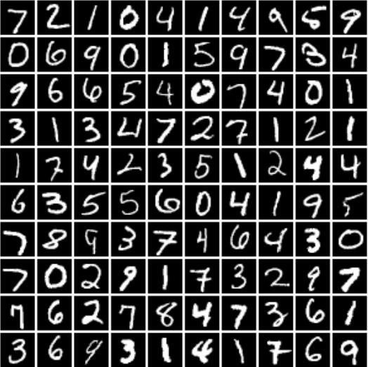
Figure 3: No noise. 100 samples

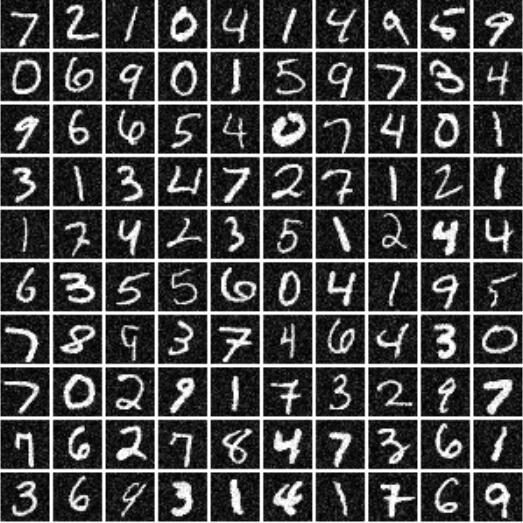
Figure 4: First level noise. 100 samples

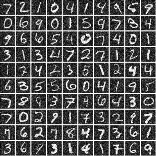
Figure 5: Second level noise. 100 samples

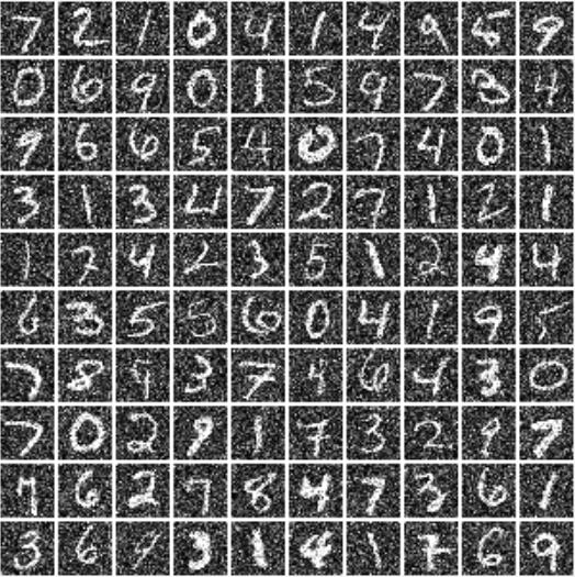
Figure 6: Third level noise. 100 samples

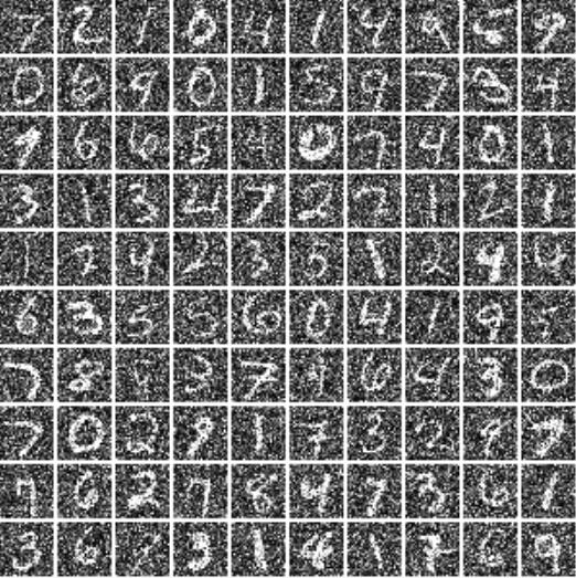
Figure 7: Fourth level noise. 100 samples

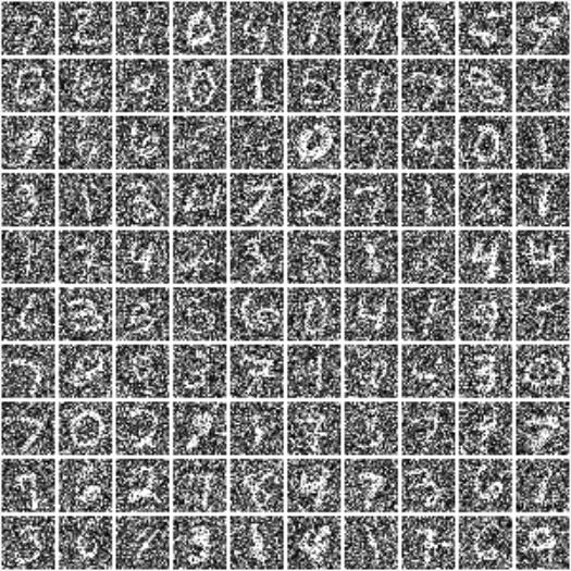
Figure 8: Fifth level noise. 100 samples

References

- [1] N. Carlini and D. Wagner, Towards Evaluating the Robustness of Neural Networks, IEEE Symposium on Security and Privacy, San Jose, CA, 39-57, 2017.
- [2] I. Goodfellow, Y. Bengio, and A. Courville, Deep Learning, MIT Press, 2016.
- [3] G. Hinton, O. Vinyals, J. Dean, Distilling the Knowledge in a Neural Network. arXiv:1503.02531, 2015.
- [4] W.V.D. Hodge and D. Pedoe. Methods of Algebraic Geometry, Volume I. Cambridge University Press, 1968.
- [5] S. Ioffe and C. Szegedy, Batch Normalization: Accelerating Deep Network Training by Reducing Internal Covariate Shift. arXiv:1502.03167, 2015.
- [6] Y. LeCun, Y. Bengio, G. Hinton, Deep Learning, Nature, 521(7553), 436-444, 2015.
- [7] M. Leshno, V.Y. Lin, A. Pinkus, S.Schocken, Multilayer Feedforward Networks with a Nonpolynomial Activation Function can Approximate any Function. Neural Networks, 6(6), 861-867, 1993.
- [8] W. Lin, Z. Yang, X. Chen, Q, Zhao, X. Li, Z. Liu, J. He, Robustness Verification of Classification Deep Neural Networks via Linear Programming. CVPR’2019, 11418-11427, 2019.
- [9] A. Madry, A. Makelov, L. Schmidt, D. Tsipras, A. Vladu, Towards Deep Learning Models Resistant to Adversarial Attacks. arXiv:1706.06083, 2017.
- [10] G. Montúfar, R. Pascanu, K. Cho, Y. Bengio, On the Number of Linear Regions of Deep Neural Networks. In NIPS’2014, 2014.
- [11] D. Molchanov, A. Ashukha, D. Vetrov, Variational Dropout Sparsifies Deep Neural Networks. arXiv:1701.05369, 2017.
- [12] S.M. Moosavi-Dezfooli, A. Fawzi, P. Frossard, DeepFool: a Simple and Accurate Method to Fool Deep Neural Networks. CVPR’2016, IEEE Press, 2016.
- [13] B. Neyshabur, R. Tomioka, N. Srebro, Norm-based Capacity Control in Neural Networks. Conference on Learning Theory, 1376-1401, 2015.
- [14] R. Socher, Y. Bengio, C.D. Manning, Deep Learning for NLP (without magic), Tutorial Abstracts of ACL’2012, 5-5, 2012.
- [15] N. Srivastava, G.E. Hinton, A. Krizhevsky, I. Sutskever, R.R. Salakhutdinov, Dropout: a Simple Way to Prevent Neural Networks from Overfitting, Journal of Machine Learning Research, 15, 1929-1958, 2014.
- [16] A. Voulodimos, N. Doulamis, A. Doulamis, E. Protopapadakis, Deep Learning for Computer Vision: A Brief Review, Computational Intelligence and Neuroscience, 2018.
- [17] L. Wan, M.D. Zeiler, S. Zhang, et al, Regularization of Neural Networks using DropConnect, International Conference on Machine Learning. 2013.
- [18] Z. Yang, X. Wang, Y. Zheng, Sparse Deep Neural Networks Using -Weight Normalization, accepted by Statistica Sinica, 2018, http://www.stat.sinica.edu.yw/statistica/.