Accelerating Finite-Temperature Kohn-Sham Density Functional Theory
with Deep Neural Networks
Abstract
We present a numerical modeling workflow based on machine learning (ML) which reproduces the total energies produced by Kohn-Sham density functional theory (DFT) at finite electronic temperature to within chemical accuracy at negligible computational cost. Based on deep neural networks, our workflow yields the local density of states (LDOS) for a given atomic configuration. From the LDOS, spatially-resolved, energy-resolved, and integrated quantities can be calculated, including the DFT total free energy, which serves as the Born-Oppenheimer potential energy surface for the atoms. We demonstrate the efficacy of this approach for both solid and liquid metals and compare results between independent and unified machine-learning models for solid and liquid aluminum. Our machine-learning density functional theory framework opens up the path towards multiscale materials modeling for matter under ambient and extreme conditions at a computational scale and cost that is unattainable with current algorithms.
I Introduction
Multiscale materials modeling [1] provides fundamental insights into microscopic mechanisms that determine materials properties. A multiscale modeling framework operating both near first-principles accuracy and across length and time scales would enable key progress in a plethora of applications. It would greatly advance materials science research—in gaining understanding of the dynamical processes inherent to advanced manufacturing [2, 3], in the search for superhard [4] and energetic materials [5, 6], and in the identification of radiation-hardened semiconductors [7, 8]. It would also pave the way for generating more accurate models of materials at extreme conditions including shock-compressed materials [9, 10] and astrophysical objects, such as the structure, dynamics, and formation processes of the Earth’s core [11], solar [12, 13, 14, 15, 16, 17, 18] and extra-solar planets[19, 20]. This requires faithfully passing information from quantum mechanical calculations of electronic properties on the atomic scale (nanometers and femtoseconds) up to effective continuum material simulations operating at much larger length and time scales. Atomistic simulations based on molecular dynamics (MD) techniques [21] and their efficient implementation [22] for large-scale simulations on high-performance computing platforms are the key link. For atomic-scale systems, MD results can be directly validated against quantum calculations. At the same time, MD can be scaled up to the much larger scales on which the continuum behaviors start to emerge (either micrometers or microseconds, or even both [23]).
MD simulations require accurate interatomic potentials (IAPs) [24]. Generating them based on machine learning (ML) techniques has only recently become a rapidly evolving research area. It has already led to several ML-generated IAPs such as AGNI [25], ANI [26], DPMD [27], GAP [28], GARFfield [29], HIP-NN [30], SchNet [31], and SNAP [32]. While these IAPs differ in their flavor of ML models, for instance, non-linear optimization, kernel methods, structured neural networks, and convolutional neural networks, they all rely on accurate training data from first-principles methods.
First-principles training datasets are commonly generated with Kohn-Sham density functional theory (DFT) [34] and its generalization to finite electronic temperature [35]. Due to its balance between accuracy and computational cost, it is the method of choice [36] for computing properties of molecules and materials with close to chemical accuracy [37, 38].
Despite its success [39], DFT is limited to the nanoscale due to its computational cost which scales as the cube of the system size. At the same time, the amount of data needed to construct an IAP increases exponentially with the number of chemical elements, thermodynamic states, phases, and interfaces [40]. Likewise, evaluation of thermodynamic properties using DFT is computationally expensive, typically to core-hours for each point on a grid of temperatures and densities [41]. Furthermore, fully converged DFT calculations at low densities, very high temperatures, or near phase transitions are considerably more difficult.
Pioneering efforts in applying ML to electronic structure calculations focus on mining benchmark databases generated from experiments, quantum chemistry methods, and DFT in order to train ML models based on kernel ridge regression and feed-forward neural networks. These efforts enabled ML predictions of molecular properties [42, 43, 44] and crystal structures [45]. Only limited efforts have gone into actually speeding up DFT calculations by directly approximating the solutions of the Kohn-Sham differential equations through ML models. Prior work has focused on approximating the kinetic energy functional using ML regression [46, 47, 48] and deep-learning models [49]. Most recently, ongoing efforts have demonstrated the usefulness of ML kernel techniques on the electronic density [50] and feed-forward neural networks on the density of states (DOS) [51, 45, 52], and the local density of states (LDOS) [53] for creating computationally efficient DFT surrogates.
In this work, we develop ML-DFT, a surrogate for DFT calculations at finite electronic temperature using feed-forward neural networks. We derive a representation of the Born-Oppenheimer potential energy surface at finite electronic temperature (Section II.1) that lends itself to an implementation within an ML workflow (Section II.2). Using the LDOS as the central quantity, ML-DFT enables us to compute the DFT total free energy in terms of a single ML model (Section II.2), applicable to coupled electrons and ions not only under ambient conditions, but also in liquid metals and plasmas. For the sake of simplicity, we will refer to the DFT total free energy as defined in Eq. (6) as total energy. Utilizing a generalization of the SNAP bispectrum descriptors on a Cartesian grid (Section II.5), the feed-forward neural network of ML-DFT (Section II.6) is trained on DFT data (Section II.3). Integrated quantities such as the band energy and the total energy of an atomic configuration at a given electronic temperature are in turn computed based on the LDOS predicted by ML-DFT. Using the LDOS in conjunction with the developed expression for total energy avoids the need to introduce another ML model to map densities to kinetic energies [50] and goes significantly beyond prior ML efforts related to the LDOS [53]. ML-DFT yields DFT-level accuracy, but comes at a negligible computational cost by avoiding the eigensolver step. We demonstrate this for aluminum (Section III). Trained on atomic configurations of aluminum at the melting point, a single ML-DFT model yields accurate results (LDOS, electronic density, band energy, and total energy) for both crystalline and liquid aluminum. Notably, band energies and total energies predicted by ML-DFT agree with the results of conventional DFT calculations to well within chemical accuracy, which is traditionally defined as 1 kcal/mol = 43.4 meV/atom. Hence, ML-DFT meets all requirements to become the backbone of the computational infrastructure needed for high-performance multiscale materials modeling of matter under ambient and extreme conditions (Section IV).
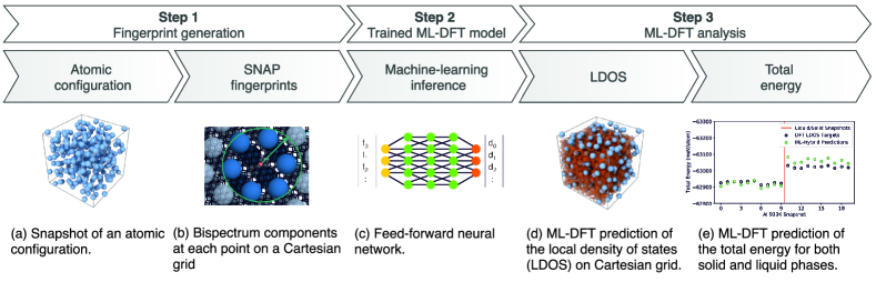
The ML-DFT workflow is illustrated in Figure 1. It starts with input data generated from finite-temperature DFT calculations for a given atomic configuration (a). SNAP fingerprints are generated for each of several million Cartesian grid points in the snapshot volume (b). Given a SNAP fingerprint as input, the trained ML-DFT feed-forward neural network makes its prediction for the LDOS vector (c). The primary output of the ML inference is the LDOS prediction at each grid point (d). Based on the predicted LDOS, quantities such as the electronic density based on Eq. (10), the DOS based on Eq. (13), and the total energy based on Eq. (9) are computed (e).
II Methods
II.1 Born-Oppenheimer Density Functional Theory at Finite Electronic Temperature
A suitable theoretical framework for computing thermodynamic materials properties from first principles is within the scope of non-relativistic quantum mechanics in the Born-Oppenheimer approximation [54]. Additionally we work within a formalism that takes the electronic temperature into account. This becomes relevant when the scale of the electronic temperature becomes comparable to the first excitation energy of the electronic system which is particularly relevant for liquid metals and plasmas. In the given framework we, hence, assume that the electrons find their thermal equilibrium on a time scale that is small compared to that of ionic motion. The formal development and implementation of such methodologies that couple electron and ion dynamics is an area of active research [55, 56, 57, 58, 59, 60, 61].
More formally, consider a system of electrons and ions with collective coordinates and , where refers to the position of the th electron, while denotes the position of the th ion of mass and charge . The physics in this framework is governed by the Born-Oppenheimer Hamiltonian
| (1) |
where denotes the kinetic energy of the electrons, the electron-electron interaction, the electron-ion interaction, and the ion-ion interaction. Note that we work within atomic units throughout, where , such that energies are expressed in Hartrees and length in Bohr radii.
Using the standard framework of quantum statistical mechanics [62], all thermodynamic equilibrium properties are formally given in terms of the grand potential
| (2) |
which is defined as a statistical average over the grand canonical operator , where denotes the particle number operator, the entropy operator, the chemical potential, and , where is the Boltzmann constant and is the electronic temperature. Statistical averages as in Eq. (2) are computed via the statistical density operator which is a weighted sum of projection operators on the underlying Hilbert space spanned by the -particle eigenstates of with energies and statistical weights . The thermal equilibrium of a grand canonical ensemble is then defined as that statistical density operator which minimizes the grand potential. Further details on the grand canonical ensemble formulation of a thermal electronic system can be found in Refs. [63, 64].
In practice, the electron-electron interaction complicates finding solutions to and, hence, evaluating the grand potential as defined in Eq. (2). Instead, a solution is found in a computationally feasible manner within DFT [34] at finite electronic temperature [35, 63, 65]. Here, a formally exact representation of the grand potential is given by
| (3) | ||||
where denotes the Kohn-Sham kinetic energy, the Kohn-Sham entropy, the classical electrostatic interaction energy, the exchange-correlation free energy which is the sum of the temperature-dependent exchange-correlation energy and the interacting entropy, the electron-ion interaction, and the ion-ion interaction. The grand potential in Eq. (3) is evaluated in terms of the electronic density defined by
| (4) |
where the sum runs over the Kohn-Sham orbitals and eigenvalues that are obtained from the solving the Kohn-Sham equations
| (5) |
where denotes the Fermi-Dirac distribution. The Kohn-Sham framework is constructed such that a noninteracting system of fermions yields the same electronic density as the interacting many-body system of electrons defined by . This is achieved by the Kohn-Sham potential which includes all electron-electron interactions on a mean-field level. While formally exact, approximations to are applied in practice either at the electronic ground state [39] or at finite temperature [66, 67, 68].
The key quantity connecting the electronic and ionic degrees of freedoms is the total energy
| (6) |
This expression yields the Born-Oppenheimer potential energy surface at finite electronic temperature, when it is evaluated as a function of . It provides the forces on the ions which are obtained from solving for the instantaneous, grand potential in thermal equilibrium for a given atomic configuration via Eq. (5). In doing so, Eq. (6) enables us to time-propagate the dynamics of the atomic configuration , in its simplest realization, by solving a Newtonian equation of motion
| (7) |
This can be further extended, for example, to take into account the energy transfer between the coupled system of electrons and ions by introducing thermostats [69, 70].
Despite its powerful utility for predicting thermodynamic and material properties on the atomic scale [37, 38] and providing benchmark data for the parameterization of IAPs for use in MD simulations [29], applying DFT becomes computationally infeasible in applications towards the mesoscopic scale due to the computational scaling of Eq. (5). The computational cost for data generation explodes exponentially with the number of chemical elements, thermodynamic states, phases, and interfaces [40] needed for the construction of IAPs.
II.2 Machine-learning Model of the Total Energy
We now reformulate DFT in terms of the LDOS which is granted by virtue of the first Hohenberg-Kohn theorem [33]. We then replace the DFT evaluation of the LDOS with a ML model for the LDOS in order to obtain all of the quantities required to evaluate the total energy while avoiding the computationally expensive solution of Eq. (5). The LDOS is defined as a sum over the Kohn-Sham orbitals
| (8) |
where denotes the energy as a continuous variable, and is the Dirac delta function. This enables us to rewrite Eq. (6) as
| (9) | ||||
where denotes the potential energy component of the XC energy [71].
The central advantage of this reformulation is that, by virtue of Eq. (9), the total energy is expressed solely in terms of the LDOS. We emphasize this by explicitly denoting the functional dependence of each term on the LDOS.
Now let us turn to the individual terms in this expression. The ion-ion interaction is given trivially by the atomic configuration. The Hartree energy , the XC energy , and the potential XC energy are all determined implicitly by the LDOS via their explicit dependence on the electronic density
| (10) |
Likewise, the band energy
| (11) |
and the Kohn-Sham entropy
| (12) | ||||
are determined implicitly by the LDOS via their explicit dependence on the DOS
| (13) |
Eq. (9) enables us to evaluate the total energy in terms of a single ML model that is trained on the LDOS and can predict the LDOS for snapshots unseen in training. This is advantageous, as it has been shown that learning energies from electronic properties, such as the density, is significantly more accurate [50] than learning them directly from atomic descriptors [72, 73, 46]. Furthermore, developing an ML model based on the LDOS instead of the density avoids complications of prior models. For example, accuracy was lost due to an additional ML model needed to map densities to kinetic energies or noise was introduced by taking gradients of the ML kinetic energy models [48, 47, 74, 75]. The two formulations in Eq. (6) and Eq. (9) are mathematically equivalent. However, Eq. (9) is more convenient in our ML-DFT workflow where we use the LDOS as the central quantity. To our knowledge, this work is the very first implementation of DFT at finite electronic temperature in terms of an ML model.
II.3 Data Generation
Our initial efforts have focused on developing an ML model for aluminum at ambient density (2.699 g/cc) and temperatures up to the melting point (933 K). The training data for this model was generated by calculating the LDOS for a set of atomic configurations using the Quantum Espresso electronic structure code [76, 77, 78]. The structures were generated from snapshots of equilibrated DFT-MD trajectories for 256 atom supercells of aluminum. We calculated LDOS training data for 10 snapshots at room temperature, 10 snapshots of the crystalline phase at the melting point, and 10 snapshots of the liquid phase at the melting point.
Our DFT calculations used a scalar-relativistic, optimized norm-conserving Vanderbilt pseudopotential (Al.sr-pbesol.upf) [79] and the PBEsol exchange-correlation functional [80]. We used a 100 Rydberg plane-wave cutoff to represent the Kohn-Sham orbitals and a 400 Rydberg cutoff to represent densities and potentials. These cutoffs resulted in a real-space grid for the densities and potentials, and we used this same grid to represent the LDOS. The electronic occupations were generated using Fermi-Dirac smearing with the electronic temperature corresponding to the ionic temperature. Monkhorst-Pack [81] k-point sampling grids, shifted to include the gamma point when necessary, were used to sample the band structure over the Brillouin zone. The DFT-MD calculations that generated the snapshots used k-point sampling for the crystalline phase and k-point sampling for the liquid phase.
In contrast, the generation of the LDOS used k-point sampling. The reason for this unusually high k-point sampling (for a 256 atom supercell) was to help overcome a challenge that arises when using the LDOS as the fundamental parameter in a ML surrogate for DFT. For a periodic supercell, the LDOS is given as
| (14) |
where the index now labels the Kohn-Sham orbitals at a particular value, and the vector index categorizes the Kohn-Sham orbitals by their transformation properties under the group of translation symmetries of the periodic supercell. In particular,
| (15) |
where is some function with the same periodicity as the periodically repeated atomic positions .
In Eq. (14), the integral with respect to is taken over the first Brillouin zone (BZ), which has volume . If this integral could be evaluated exactly, the resulting LDOS would be a continuous function of with Van Hove singularities [82] of the form or at energies that correspond to critical points of the band structure . However, when this integral is represented as a summation over a finite number of k-points , as in the Monkhorst-Pack [81] approach used in our calculations, it is necessary to replace the Dirac delta function appearing in Eq. (14) with a finite-width representation . The LDOS used to train our ML model is then obtained by evaluating
| (16) |
on a finite grid of values. In our calculations, we use an evenly spaced grid with a spacing of 0.1 eV, a minimum value of -10 eV, and a maximum value of +15 eV. Hence, the data for each grid point consists of a vector of 250 scalar values. Kohn-Sham orbitals with eigenvalues significantly outside the energy range where we evaluate the LDOS make negligible contributions to the calculated LDOS values, and ideally we would include a sufficient number of the lowest Kohn-Sham orbitals in Eq. (14) and Eq. (16) to span this energy range. However, due to memory constraints on our k-point DFT calculations, we were only able to calculate orbitals. At ambient density, this provides an accurate LDOS up to eV, and the relevant Fermi levels are at eV. The tails of should be negligible above eV for K. At higher electronic temperatures, it would become necessary to increase when generating the training data in order to get an accurate LDOS over a wider energy range.
The challenge mentioned above arises in the choice of the delta function representation and the k-point sampling scheme for a given grid. If the function is too wide, it leads to systematic errors in the LDOS and derived quantities such as the density, band energy and total energy. However, if is too narrow or too few k-points are used to sample the BZ, then only a few values of make substantial contributions to the LDOS at each point on the grid, and there is a large amount of noise in the resulting LDOS.
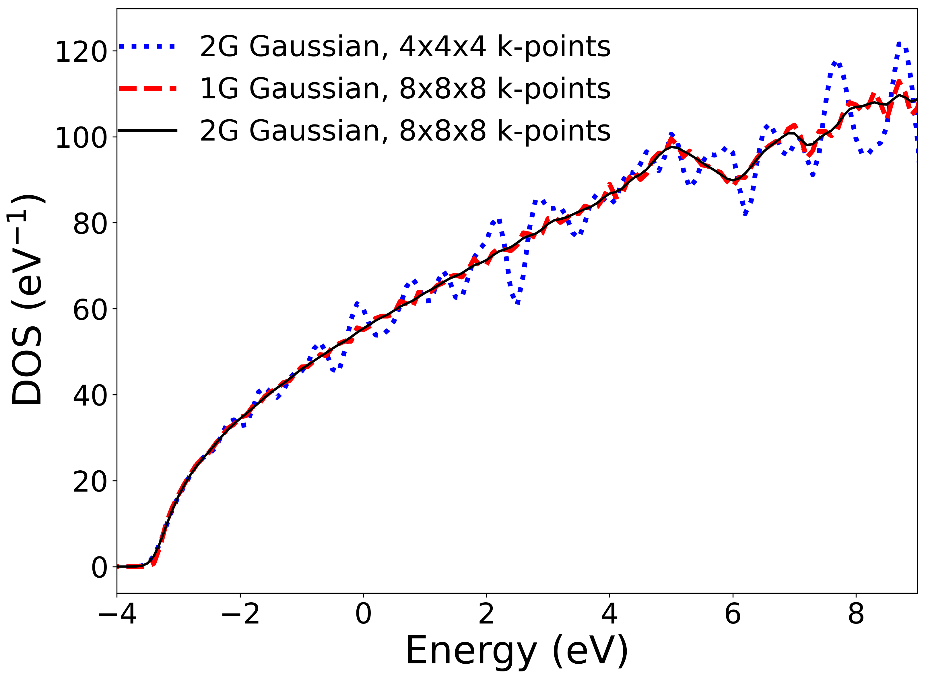
Figure 2 demonstrates these trade-offs for a Gaussian representation by plotting the DOS in the upper panel and the error in the band energy calculated from the DOS in the lower panel. The top panel shows that using fewer k-points or a narrower leads to unphysical noise in the calculated DOS, while the bottom panel shows that using a wider leads to an increasing error in the band energy. The lower panel also shows that the noise in the DOS that arises with a narrower is reflected in an increasing variability in the band energy error.
Since a larger k-point sampling allows a narrower to be used without introducing excessive noise into the LDOS, we can minimize the errors in quantities calculated from the LDOS by using as many k-points as possible. In the LDOS calculations used to train our ML model, we used k-point sampling, which was the largest k-point sampling that was computationally tractable for our 256 atom cells. We then chose a Gaussian with eV (indicated in the lower panel of Figure 2), which gives a relatively small and very consistent error in derived quantities. For example, the average error in the band energies calculated from the resulting LDOS (relative to fully converged DFT) is -4.483 meV/atom when the average is taken over all of our snapshots. The average error becomes -4.466, -4.500, and -4.483 meV/atom when the average is restricted to the 298K, 933K solid, and 933K liquid snapshots, respectively. These results show that the error changes very little between different temperatures and structures. These errors are also very consistent for different structures at the same temperature and phase. In particular, the root mean square variations in the errors are 0.004, 0.011, and 0.017 meV/atom for the 298K, 933K solid, and 933K liquid snapshots respectively. Our choices for the grid spacing and the width of the Gaussian broadening turn out to be similar to those made in Ref. [52].
In electronic structure calculations, consistent errors in calculated energies (for example, the errors due to incomplete convergence with respect to the plane-wave cutoffs in traditional DFT calculations) are generally not a problem. Instead, quantities of interest almost always involve the difference between two energies, and thus it is the variation of the errors between different structures that affects actual results. With the k-point sampling and the choice of described above, the errors differ by only about one-thousandth of the room-temperature thermal energy, and such consistent errors are very unlikely to impact quantities of interest. Furthermore, these errors are independent of the errors introduced by using ML to approximate the LDOS. In particular, a perfect ML approximation would reproduce the results calculated from the DFT LDOS (defined in the same manner as in the generation of our training data) rather than the results calculated by exact DFT. Finally, we believe that further work will be able to identify methods that use DFT to calculate even more accurate LDOS training data with less computational effort than our k-point calculations. Some ideas include Fourier interpolation of the Kohn-Sham bands and orbitals, or an approach analogous to the tetrahedron method [83]. The remainder of this paper will focus on the effects of approximating the LDOS with ML. In light of the above considerations, errors will be quoted relative to results calculated from the DFT LDOS rather than exact DFT.
II.4 Evaluation of Energies from the Local Density of States
A key step in calculating the total energy defined in Eq. (9) from the LDOS is the evaluation of several integrals in Eqs. (10), (11), and (12) that have the form
| (17) |
for some function . The evaluation of Eq. (17) poses a challenge, because changes rapidly compared to in several cases of interest. We provide a solution in terms of an analytical integration, as illustrated in Appendix A. Given our analytical integration technique, it is straightforward to evaluate the total energy using Eq. (9) and the standard methods of DFT in an accurate and numerically stable manner.
II.5 Fingerprint Generation
We assume that the LDOS at any point in space can be approximated by a function that depends only on the positions and chemical identities of atoms within some finite neighborhood of the point. In order to approximate this function using ML, we need to construct a fingerprint that maps the neighborhood of any point to a set of scalar values called descriptors. On physical grounds, good descriptors must satisfy certain minimum requirements: (i) invariance under permutation, translation, and rotation of the atoms in the neighborhood and (ii) continuous differentiable mapping from atomic positions to descriptors, especially at the boundary of the neighborhood. While these requirements exclude some otherwise appealing choices, such as the Coulomb matrix [84], the space of physically valid descriptors is still vast. In the context of ML-IAPs, the construction of good atomic neighborhood descriptors has been the subject of intense research. Recent work by Drautz [85] has shown that many prominent descriptors [86, 87, 88] belong to a larger family that are obtained from successively higher order terms in an expansion of the local atomic density in cluster integrals. The SNAP bispectrum descriptors [32] that we use in this work correspond to clusters of three neighbor atoms yielding four-body descriptors.
In contrast to prior work on ML-IAPs in which descriptors are evaluated on atom-centered neighborhoods, here we evaluate the SNAP descriptors on the same Cartesian grid points at which we evaluated the LDOS training data (see Eq. (16) above). For each grid point, we position it at the origin and define local atom positions in the neighborhood relative to it. The total density of neighbor atoms is represented as a sum of -functions in a three-dimensional space:
| (18) |
where is the position of the neighbor atom of element relative to the grid point. The coefficients are dimensionless weights that are chosen to distinguish atoms of different chemical elements , while a weight of unity is assigned to the location of the LDOS point at the origin. The sum is over all atoms within some cutoff distance that depends on the chemical identity of the neighbor atom. The switching function ensures that the contribution of each neighbor atom goes smoothly to zero at . Following Bartók et al. [87], the radial distance is mapped to a third polar angle defined by
| (19) |
The additional angle allows the set of points in the 3D ball of possible neighbor positions to be mapped on to the set of points on the unit 3-sphere. The neighbor density function can be expanded in the basis of 4D hyperspherical harmonic functions
| (20) |
where and are rank complex square matrices, are Fourier expansion coefficients given by the inner product of the neighbor density with the basis functions of degree , and the symbol indicates the scalar product of the two matrices. Because the neighbor density is a weighted sum of -functions, each expansion coefficient can be written as a sum over discrete values of the corresponding basis function
| (21) |
The expansion coefficients are complex-valued and they are not directly useful as descriptors because they are not invariant under rotation of the polar coordinate frame. However, scalar triple products of the expansion coefficients
| (22) |
are real-valued and invariant under rotation [87]. The symbol indicates a Clebsch-Gordan product of matrices of rank and that produces a matrix of rank , as defined in our original formulation of SNAP [88]. These invariants are the components of the bispectrum. They characterize the strength of density correlations at three points on the 3-sphere. The lowest-order components describe the coarsest features of the density function, while higher-order components reflect finer detail. The bispectrum components defined here have been shown to be closely related to the 4-body basis functions of the Atomic Cluster Expansion introduced by Drautz [85].
For computational convenience, the LAMMPS implementation of the SNAP descriptors on the grid includes all unique bispectrum components with indices no greater than . For the current study we chose , yielding a fingerprint vector consisting of 91 scalar values for each grid point. The cutoff distance and element weight for the aluminum atoms were set to 4.676 Å and , respectively.
II.6 Machine-learning Workflow and Neural Network Model
| 1. | Training data generation |
| (i.) | Run MD simulation to obtain atomic configurations at a specific temperature and density. |
| (ii.) | Run Quantum Espresso DFT calculation on the atomic configurations. |
| (iii.) | Perform Quantum Espresso post-processing of the Kohn-Sham orbitals to obtain the LDOS on the Cartesian grid. |
| (iv.) | Generate SNAP fingerprints on a uniform Cartesian grid from the atomic configurations. |
| 2. | ML-DFT model training |
| (i.) | Training/validation set, ML model, and initial hyperparameter selection. |
| (ii.) | Normalization/standardization of the training data. |
| (iii.) | Train ML-DFT model to convergence. |
| (iv.) | Adjust hyperparameters for increased accuracy and repeat training for a new model. |
| 3. | ML-DFT analysis |
| (i.) | Evaluate unseen test snapshots on trained and tuned ML-DFT models. |
| (ii.) | Calculate quantities of interest from the LDOS predicted by ML-DFT. |
Neural network models, especially deep neural networks, are profoundly successful in numerous tasks, such as parameter estimation [89, 90], image classification [91, 92], and natural language processing [93, 94]. Moreover, neural networks may act as function approximators [95, 96]. A typical feed-forward neural network is constructed as a sequence of transformations, or layers, with the form:
| (23) |
where is the intermediate column-vector of length at layer , is a matrix of size , is a bias vector of length , and is the next column-vector of length in the sequence. The first and the last layers accept input vectors, , and produce output predictions, , respectively. There can be any arbitrary number of hidden layers constructed between the input layer and the output layer. After each layer, a non-linear activation unit transforms its input. The composition of these layers is expected to learn complex, non-linear mappings.
Given a dataset of input vectors and target output vectors, (, ), we seek to find the optimal and , , such that the neural network minimizes the root mean squared loss between the neural network predictions and targets . In this work, the network predicts LDOS at each grid point using the SNAP fingerprint as input. The specific feed-forward networks we consider have input fingerprint vectors of length 91 scalar values and output LDOS vectors of length 250 scalar values. The grid points are defined on a uniform Cartesian grid, or 8 million total points per snapshot.
Neural network models are created in two stages: training and validation, using separate training and validation datasets. The training phase performs gradient-based updates, or backpropagation [96], to and using a small subset, or mini-batch, of column vectors in the training dataset. Steps taken in the direction of the gradient are weighted by a user provided learning rate (LR). Successive updates incrementally optimize the neural network. An epoch is one full pass through the training dataset for the training phase. After each epoch, we perform the validation phase, which is an evaluation of the current model’s accuracy on a validation dataset. The training process continues alternating between training and validation phases until an early stopping termination criterion [97] is satisfied. Early stopping terminates the learning process when the root mean squared loss on the validation dataset does not decrease for a successive number of epochs, or patience count. Increasing validation loss indicates that the model is starting to over-fit the training dataset and will have worse generalization performance if the training continues.
Next, the hyperparameters, which determine the neural network architecture and optimizer specifications, must be optimized to maximize model accuracy (and minimize loss). Due to the limited throughput, we make the assumption that all hyperparameters are independent. Independence allows the hyperparameter tuning to optimize one parameter at a time, greatly reducing the total rounds of training. We then ensure local optimality of the hyperparameter minimizer by direct search [98].
The ML-DFT model uses as input vectors the SNAP fingerprints defined at real-space grid points. The target output vectors of the ML-DFT model are the Quantum Espresso generated LDOS vectors defined at the corresponding real-space grid points. Importantly, each fingerprint and LDOS vector is treated as independent of any other grid point. Further, the training data may include multiple aluminum snapshots, in which case the number of grid points is equal to the number of snapshots times the number of grid points per snapshot. No distinction is made in the model by grid points belonging to separate snapshots. The validation snapshot is always a full set of grid points from a single snapshot.
For inference, all remaining snapshots are used to test the generalization of the ML-DFT model. Consider a single snapshot where we wish to predict the total energy. At each grid point, a SNAP fingerprint vector is used to predict an LDOS vector. Using the steps in Section II.4 and Appendix A, the full set of ML predicted LDOS vectors produce a total energy.
In summary, the ML-DFT training workflow is provided in Table 1. The ML-DFT models are built on top of the PyTorch [99] framework and the Numpy [100] and Horovod [101] packages. PyTorch provides the necessary infrastructure for neural network construction and efficiently running the training calculations on GPU machines. The Numpy package contains many performant tools for manipulating tensor data, and the Horovod package enables data-parallel training for MPI-based scalability.
III Results

The difficulty of predicting the electronic structure of materials is strongly dependent on the diversity of local atomic configurations considered in training and testing. During the development stage of this work we focused on the relatively simple case of solid aluminum at ambient temperature and density (298 K, 2.699 g/cm3). We then turned our attention to the more challenging case of solid and liquid aluminum near the melting point (933 K, 2.699 g/cm3) and we present results for that case here.
Specifically, we train and tune a collection of unique ML-DFT models for each temperature. In the 298 K case, we train a single model using 1 snapshot, validate on 1 snapshot, and test on 8 snapshots. At 933 K, we train 8 models with different combinations of liquid and solid snapshots as the training set. The first 3 cases use 4 training snapshots with either 4 liquid snapshots, 4 solid snapshots, or 2 liquid and 2 solid snapshots. The second 3 cases, similarly, use 8 training snapshots with either 8 liquid, 8 solid, or 4 liquid and 4 solid snapshots. Finally, there are two models that use 8 or 12 training snapshots and a validation set that include both liquid and solid snapshots. Each 933 K model created is then tested on the remaining 933 K snapshots. In order to study the variability in LDOS between the three groups (298 K solid, 933 K solid, and 933 K liquid), we reduce the dimensionality of the LDOS datasets and study them using principal component analysis (PCA).
Further technical details on fingerprint generation, neural network architecture, ML training, optimization of hyper-parameters, and the variability in LDOS outputs are given in Appendix B. We provide results for the ambient case in Appendix C.
III.1 Local Density of States Predictions for Solid and Liquid Aluminum from ML-DFT
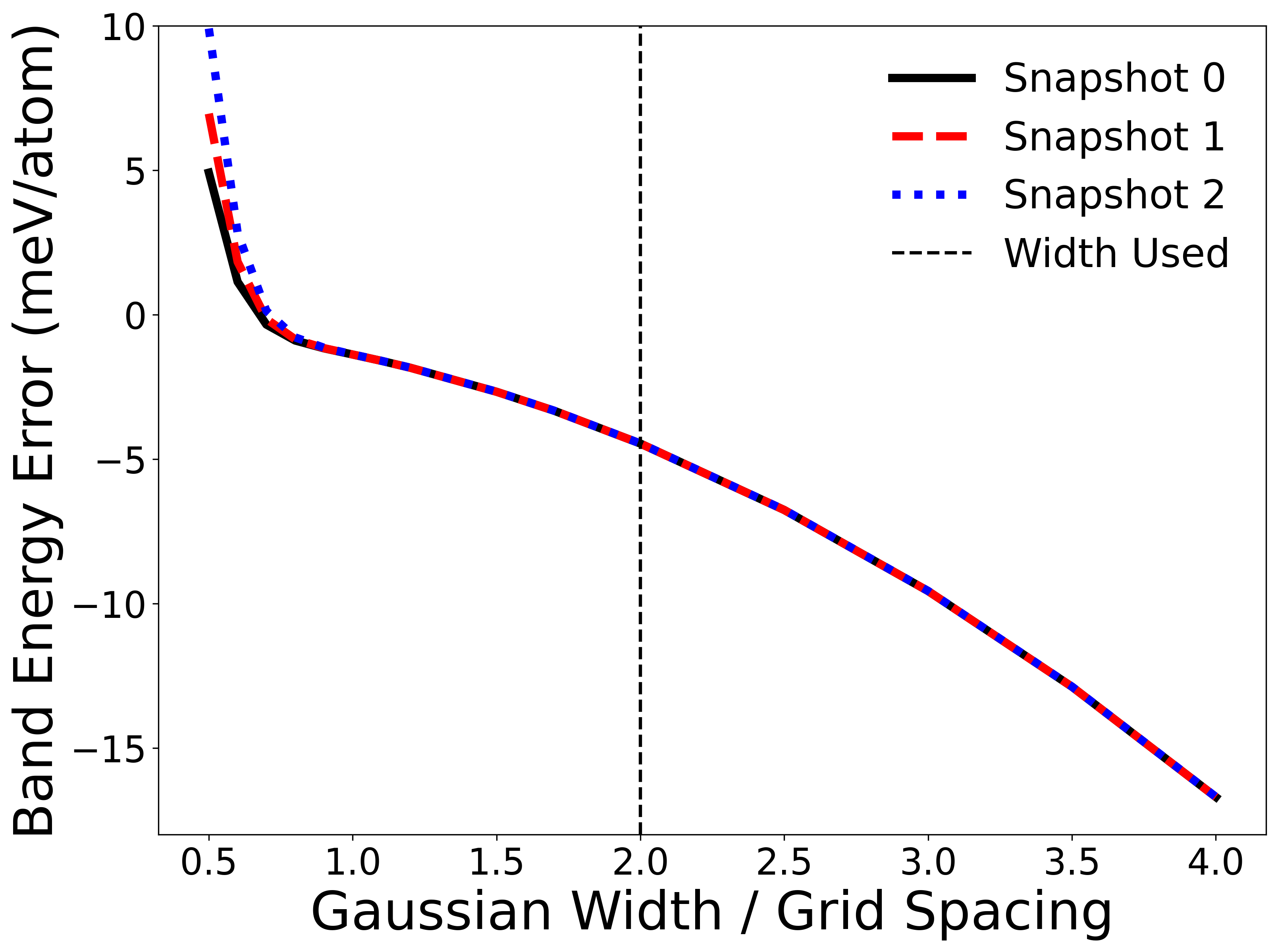
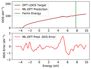
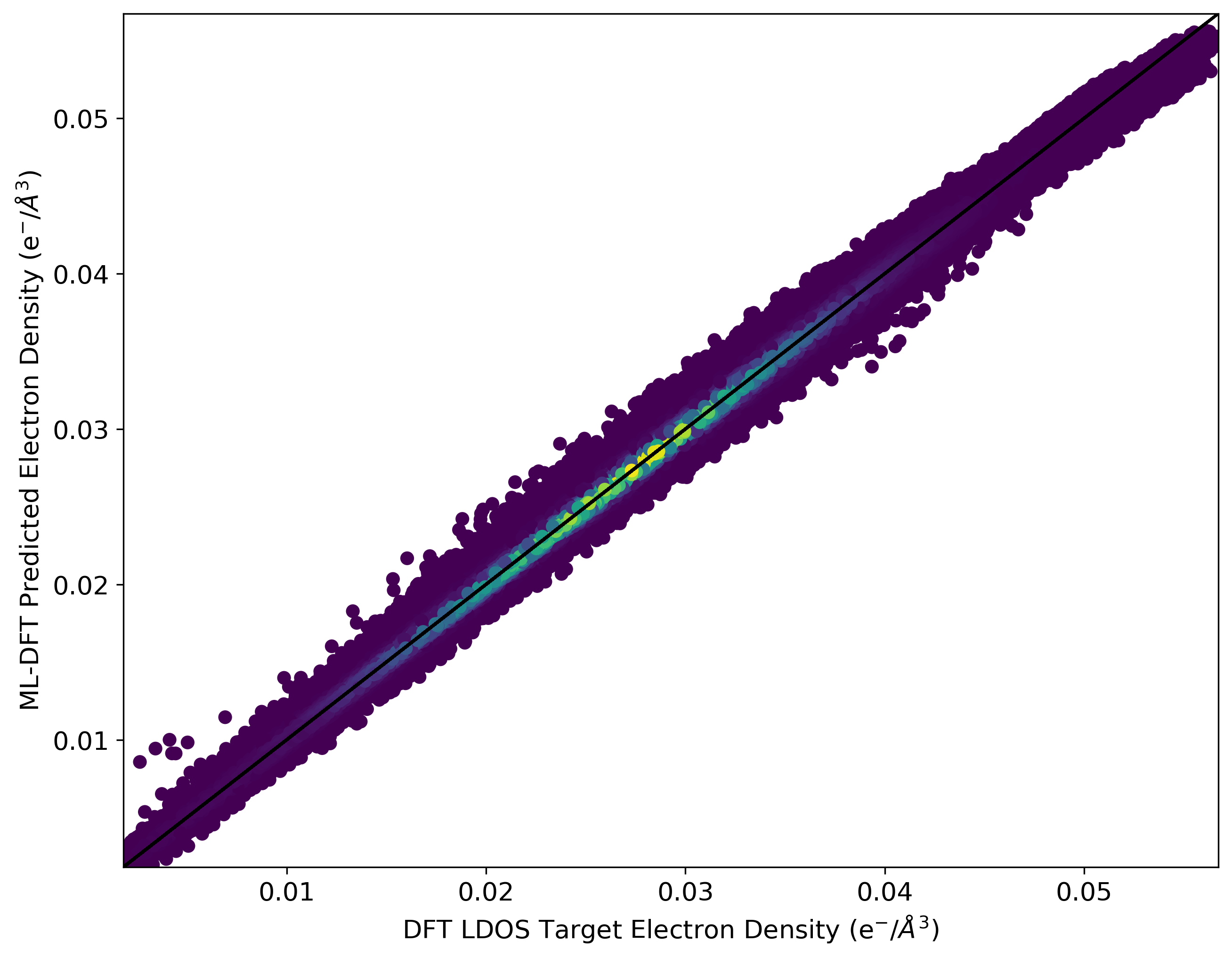
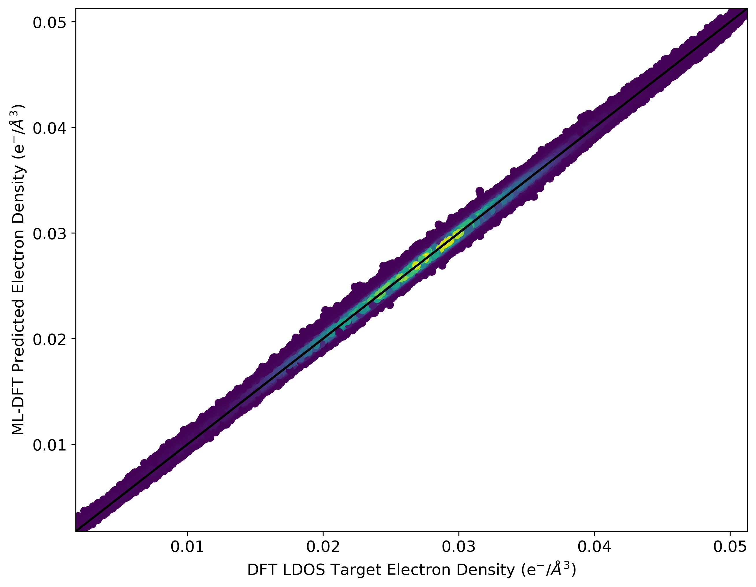
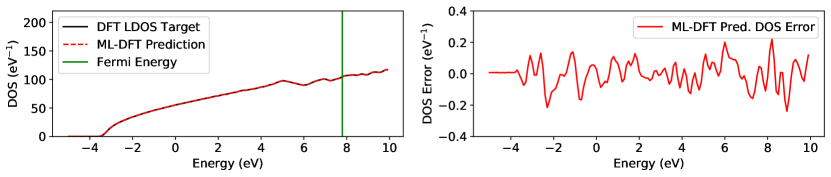
First we assess the accuracy of ML-DFT for spatially resolved and energy resolved quantities. To this end, Figure 3 illustrates the DOS and its errors in the relevant energy range from -5 to 10 eV, where the Fermi energy is at 7.689 eV in the liquid and 7.750 eV in the solid phase. The DOS prediction is computed from Eq. (13) using the ML-DFT predicted LDOS. In both liquid (left) and solid (right) phases, the ML-DFT model reproduces the DOS to very high accuracy. The illustration of the errors (bottom panels) confirms the ML-DFT model’s accuracy and shows the absence of any unwanted error cancellation over the energy grid. Figure 3 also shows that the Van Hove singularities [82] at and above eV, which show up strongly in the 298K DOS in Figure 2, are noticeably smeared out by thermal fluctuations in the atomic positions in the 933 K solid-phase DOS and essentially gone in the 933 K liquid. Figure 4 shows the DFT target electronic density versus the predicted electronic density for both liquid (left) and solid (right) phases at each point on the Cartesian grid. The frequency of the predicted results is indicated by the marker color. The ML-DFT prediction is computed from Eq. (10) using the ML-DFT predicted LDOS. The alignments of the predictions along the diagonal exhibit small standard deviations for the liquid and solid test snapshot. It illustrates how well the ML-DFT model reproduces the electronic density in a systematic manner with high accuracy, despite the fact that the electronic structure is qualitatively very distinct in the solid and liquid phases of aluminum. Furthermore, maximum absolute errors for the liquid and solid test snapshot are 0.00601 and 0.00254 , respectively. The mean absolute errors are an order of magnitude lower at 0.000284 and 0.000167 , respectively. The mean absolute percentage errors are 1.12% and 0.66%, respectively.
III.2 Single-phase Solid and Liquid Aluminum ML-DFT Models
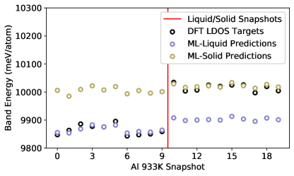
We demonstrate the errors in total energy and band energy on models trained on data from the same phase, either solid or liquid. Figure 5 and Table 2 show these results. When training, validation, and test sets are all from the same phase, either solid or liquid, the overall ML-DFT accuracy is very high. The mean absolute error in the total energy for the 8 snapshot liquid model is 9.31 meV/atom. Moreover, the 8 snapshot solid model has a mean absolute error of 15.71 meV/atom. In both cases, the main contribution to the error is due to the band energy error which is 5.21 meV/atom in the liquid test set and 13.37 meV/atom in the solid. Both models have a similar mean absolute percentage error, 0.01% in the liquid model and 0.03% in the solid model.
However, training on a single phase results in poor predictive accuracy for the phase unseen in training, as is shown clearly in Figure 5 and Table 2. For the ML-DFT model trained on 8 liquid snapshots, the mean absolute total energy error in the solid test set rises to 111.41 meV/atom. For the model trained on 8 solid snapshots, the mean absolute total energy error in the liquid test set rises to 123.29 meV/atom. Again, the major contribution to the error stems from the band energy which is 113.40 meV/atom in the solid test set and 139.96 meV/atom in the liquid.
III.3 Hybrid Liquid-Solid Aluminum ML-DFT Models
| Training Set | Test Set | Band Energy | Total Energy | ||||
| (Validation Set) | Max. AE | MAE | MAPE | Max. AE | MAE | MAPE | |
| (meV/atom) | (meV/atom) | (%) | (meV/atom) | (meV/atom) | (%) | ||
| 4 Liquid | 5 Liquid | 13.57 | 9.80 | 0.0994 | 12.39 | 7.13 | 0.0113 |
| (1 Liquid) | 10 Solid | 113.50 | 100.84 | 1.0067 | 106.62 | 91.54 | 0.1452 |
| 8 Liquid | 1 Liquid | 5.21 | 5.21 | 0.0529 | 9.31 | 9.31 | 0.0148 |
| (1 Liquid) | 10 Solid | 126.69 | 113.40 | 1.1320 | 125.07 | 111.41 | 0.1768 |
| 4 Solid | 10 Liquid | 142.63 | 126.99 | 1.2875 | 142.95 | 126.78 | 0.2015 |
| (1 Solid) | 5 Solid | 13.15 | 8.44 | 0.0843 | 14.45 | 9.81 | 0.0156 |
| 8 Solid | 10 Liquid | 158.25 | 139.96 | 1.4190 | 153.45 | 123.29 | 0.1959 |
| (1 Solid) | 1 Solid | 13.37 | 13.37 | 0.1336 | 15.71 | 15.71 | 0.0249 |
| 2 Liquid + 2 Solid | 8 Liquid | 73.76 | 62.14 | 0.6299 | 57.34 | 48.47 | 0.0770 |
| (1 Solid) | 7 Solid | 37.26 | 28.22 | 0.2816 | 41.53 | 29.50 | 0.0468 |
| 4 Liquid + 4 Solid | 6 Liquid | 67.28 | 58.23 | 0.5906 | 61.29 | 51.37 | 0.0816 |
| (1 Solid) | 5 Solid | 25.33 | 16.16 | 0.1613 | 26.98 | 15.11 | 0.0240 |
| 4 Liquid + 4 Solid | 5 Liquid | 36.84 | 28.54 | 0.2896 | 28.39 | 21.33 | 0.0339 |
| (1 Liquid + 1 Solid) | 5 Solid | 44.94 | 37.19 | 0.3711 | 47.30 | 38.57 | 0.0612 |
| 6 Liquid + 6 Solid | 3 Liquid | 21.34 | 17.11 | 0.1737 | 15.76 | 13.04 | 0.0207 |
| (1 Liquid + 1 Solid) | 3 Solid | 39.33 | 33.56 | 0.3354 | 39.23 | 31.60 | 0.0501 |
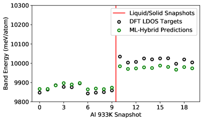
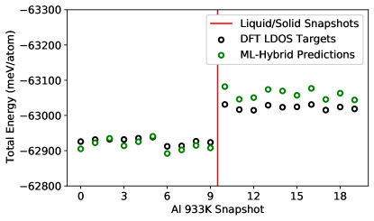
In Figure 6 and Table 2 we demonstrate our central result, a single ML-DFT model that is capable of yielding accurate results for both liquid and solid aluminum at a temperature of 933 K with accuracy sufficient for meaningful atomistic simulations of electronic, thermodynamic, and kinetic behavior of materials. Using the hyperparameters listed in Table 3, the most accurate dual-phase hybrid ML-DFT model was trained using 6 liquid and 6 solid snapshots (snapshots 0–5 and 10-15) as the training dataset and 1 solid and 1 liquid snapshot (snapshots 6 and 16) as a validation set. This ML-DFT model achieves state-of-the-art ML accuracy for all test snapshots considered.
Overall, Table 2 summarizes the total energy (Eq. 9) and band energy (Eq. 11) errors for each of the eight ML-DFT models. Training and validation sets determine the specific ML-DFT model and the test sets are used to measure the model’s ability to generalize to liquid or solid phase snapshots.
Most notably, our overall most accurate hybrid ML-DFT model predicts the total energy over both solid and liquid phases with a mean absolute error of 13.04 meV/atom in the solid test set and 31.60 meV/atom in the liquid test set, as illustrated in Figure 6 and listed in the last row of Table 2. In comparison with the single-phase ML-DFT models in Figure 5, the hybrid ML-DFT model is able to generalize to both liquid and solid snapshots. This is adequate to resolve the solid-liquid total energy difference (110 meV/atom) and is approaching the 5 meV/atom accuracy of the best ML-IAPs used in large-scale MD simulations [102].
Furthermore, the sensitivity of ML-DFT towards the volume of training data is also assessed in Table 2. Reducing the training dataset to only 2 liquid and 2 solid snapshots degrades the accuracy for both the band and total energies as expected. While the mean absolute error of 29.50 meV/atom in the solid phase is about the same as in the larger training set, the error in the liquid phase rises to 48.47 meV/atom. This emphasizes the fact that a desired accuracy in the ML-DFT model can be approached systematically by increasing the volume of training data.
Interestingly, in Figure 6, the training snapshots do not necessarily have the lowest error as might be expected. The band and total energy errors for training snapshot 0, for example, are slightly larger than the errors for test snapshots 8 and 9. For the solid snapshots, both training snapshots (10–15) and test snapshots (17–19) have very similar errors in both the band energy and total energy. Similar observations can be made for Figure 5. A greater number of liquid and solid test snapshots will only further refine the statistics of the ML-DFT model accuracy. Future investigations will include both sensitivity analysis and thorough validation of the ML-DFT model, particularly in the context of large-scale MD simulations.
IV Discussion
In the present work, we establish an ML framework that eliminates the most computationally demanding and poorly scaling components of DFT calculations. Once trained with DFT results for similar systems, it can predict many of the key results of a DFT calculation, including the LDOS, DOS, density, band energy, and total energy, with good accuracy. After training, the only input required by the model is the atomic configuration, i.e., the positions and chemical identities of atoms. We have been able to train a single model that accurately represents both solid and liquid properties of aluminum. The ML-DFT model is distinct from previous ML methodologies, as it is centered on materials modeling in support of accurate MD-based predictions for the evolution of both electronic and atomic properties. We represent materials descriptors (such as the LDOS) on a regular grid as opposed to basis functions [50] and use a specific formulation in terms of the LDOS to reconstruct the total energy. Our approach also generalizes to non-zero electronic temperatures in a straightforward way, which allows it to be easily applied to materials at extreme conditions.
Furthermore, the very recently published work [53] stopped short of demonstrating that the ML-predicted LDOS can be utilized to accurately calculate energies and forces needed to enable MD calculations. Further work on computing accurate forces of materials under elevated temperatures and pressures will follow, as well as a detailed exploration of ML-DFT’s accuracy when scaled to O() atoms, well beyond the reach of standard DFT.
Acknowledgments
Sandia National Laboratories is a multimission laboratory managed and operated by National Technology & Engineering Solutions of Sandia, LLC, a wholly owned subsidiary of Honeywell International Inc., for the U.S. Department of Energy’s National Nuclear Security Administration under contract DE-NA0003525. This paper describes objective technical results and analysis. Any subjective views or opinions that might be expressed in the paper do not necessarily represent the views of the U.S. Department of Energy or the United States Government. This work was partly funded by the Center for Advanced Systems Understanding (CASUS) which is financed by the German Federal Ministry of Education and Research (BMBF) and by the Saxon State Ministry for Science, Art, and Tourism (SMWK) with tax funds on the basis of the budget approved by the Saxon State Parliament. We thank Warren Davis and Joshua Rackers for helpful conversations and Mitchell Wood for visualizing the SNAP fingerprint grid.
Appendix A Analytical Evaluation of Derived Quantities from the Local Density of States
Consider the numerically challenging integral in Eq. (17). When , this integral gives the electronic density and the total number of electrons, when the result is the band energy, and when we obtain the entropy contribution to the energy. When , Eq. (17) results in a scalar quantity, and we can evaluate the total number of electrons, the band energy, or the entropy contribution to the total energy. Alternatively, when , Eq. (17) results in a field that depends on the position with the electronic density being the most important result.
Our ML model gives us evaluated on a grid of energy values . We will extend to a defined for all between and by linear interpolation. This allows us to perform the required integrals analytically. It is necessary to treat these integrals carefully because changes rapidly compared to for many systems of interest. In particular, changes from one to zero over a few , while the spacing of the grid is several times at room temperature. In order to evaluate these integrals analytically, we can use the representation of and in terms of the polylogarithm special functions
| (24) | ||||
| (25) |
where . It is useful to define a series of integrals giving moments of and with respect to and evaluate these integrals using integration by parts and the properties of . In particular, the relationship
| (26) |
is useful. The required integrals are
| (27) | ||||
| (28) | ||||
| (29) | ||||
| (30) | ||||
| (31) | ||||
Quantities of interest with the form of Eq. (17) can then be evaluated as a weighted sum over the DOS or LDOS evaluated at the energy grid points
| (32) |
where the weights are given by
| (33) | ||||
When , and , we obtain , the total number of electrons in the system. The Fermi level is then adjusted until is equal to the total number of valence electrons in the system (i.e., the system is charge neutral). When and , we obtain , and we can easily obtain the band energy by adding . When and , we obtain , the entropy contribution to the energy. Finally, when , and , we obtain , the electronic density. Given these quantities, it is straightforward to evaluate the total (free) energy using Eq. (9) and the standard methods of DFT.
Appendix B Machine-learning Model Details
| Model | 298K | 933K |
|---|---|---|
| Parameter | Model | Models |
| FP length | 91 | 91 |
| FP scaling | Elem.-wise stand. | Elem.-wise stand. |
| LDOS length | 250 | 250 |
| LDOS scaling | Max norm. | Max norm. |
| Optimizer | Adam | Adam |
| Minibatch size | 1000 | 1000 |
| Learning rate (LR) | 1e-5 | 5e-5 |
| LR schedule | 4 epochs | 4 epochs |
| Early stopping | 8 epochs | 8 epochs |
| Max layer width | 800 | 4000 |
| Layers | 5 | 5 |
| Activation Func. | LeakyReLU | LeakyReLU |
| Total weights | 1.62e6 | 3.34e7 |
The 298 K systems include 10 snapshots of SNAP fingerprint and Quantum Espresso LDOS data. At 933 K, there are 10 snapshots of liquid aluminum and 10 snapshots of solid aluminum. For the fingerprints and LDOS data, each snapshot uses the same uniform Cartesian real-space grid, ( points). Each snapshot, including both SNAP fingerprint and LDOS data, is 20.7 gigabytes.
We observe that the 933 K ML-DFT models require a greater amount of training data. Furthermore, the optimized 298 K model requires approximately 1.6 million weights, whereas the 933 K models require 33.4 million weights. The larger training set and greater model complexity can be attributed to greater LDOS variability at the higher temperature.
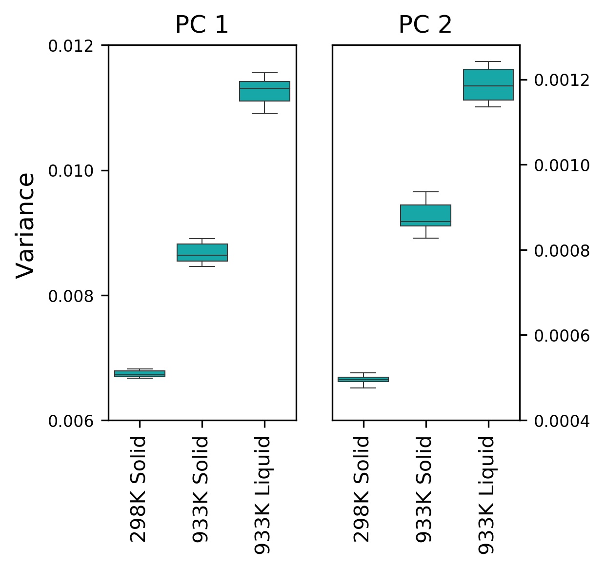
To facilitate comparing LDOS variability between the three groups (298 K solid, 933 K solid, and 933 K liquid), the dimensionality of the LDOS datasets was reduced using principal component analysis (PCA). Because of the large amount of data ( samples by 250 energy levels), PCA was performed incrementally using the scikit-learn Python package [103]. The resulting first principal component explained approximately 81.7% of the variance in the LDOS, and the second explained an additional 7.9%.
The variance of the first two principal component scores was calculated for each of the 30 snapshots. Figure 7 shows these variances grouped by snapshot temperature and phase. 933 K liquid snapshots are seen to possess the highest variance, followed by the 933 K solid snapshots. The 298 K solid snapshots have the lowest variance.
| Training Set | Test Set | Band Energy | Total Energy | ||
| (Validation Set) | Max. AE | MAE | Max. AE | MAE | |
| (meV/atom) | (meV/atom) | (meV/atom) | (meV/atom) | ||
| 1 Solid | 8 Solid | 3.82 | 2.48 | 5.60 | 3.07 |
| (1 Solid) | |||||
| Step | Time (s) | Time (s) | Optimization notes |
|---|---|---|---|
| 298K Model | 933K Model | ||
| Generate fingerprint vectors from atomic positions | 2909.75 | 2908.12 | LAMMPS used only in serial mode, speedup possible by using parallelization |
| Load modules | 0.36 | 0.36 | – |
| Infer LDOS from neural network | 18.72 | 53.94 | Only a single GPU was used |
| Integrate LDOS to DOS | 1.57 | 1.44 | – |
| Determine Fermi level | 2.23 | 2.40 | – |
| Integrate LDOS to Density | 1282.39 | 1277.66 | Integration unoptimized and in serial |
| Evaluate total energy contributions from DOS | 0.96 | 0.99 | – |
| Evaluate total energy contributions from density | 87.50 | 87.17 | Quantum Espresso used only in serial mode, speedup possible by using parallelization |
We perform a sequence of hyperparameter tunings once for each temperature using the optimization strategy described in Section II.6. The final 933 K models are trained using the same hyperparameters. Further accuracy may be obtainable once training throughput is increased and multiple, independent hyperparameter optimizations are made possible. The optimized ML-DFT model parameters are given in Table 3. Scaling of the input and output data prior to training is critical to ML-DFT model accuracy. We perform an element-wise standardization to mean 0 and standard deviation 1 for the fingerprint inputs. For example, standardize the first scalar of all fingerprint vectors in the training set, then standardize the second scalar of all fingerprints, and so on. For the LDOS outputs, we perform a normalization using the maximum LDOS value of the entire training dataset.
The hyperparameter convergence for the 298 K and 933 K models required 48 and 23 training iterations, respectively. Once the 298 K case was optimized, using those optimized hyperparameters as the 933 K optimization’s initial iterate greatly accelerated convergence resulting in fewer training iterations. Within an iteration, the 298 K model requires 93 epochs. For the 8 snapshot 933 K cases, the single phase models, either liquid or solid, required just 39–50 epochs to converge. Comparatively, the final hybrid liquid-solid model required 101 epochs to converge.
Due to the large quantity of training data in the 933 K case (12 training 2 validation snapshot 20.7 gigabytes), the required training strategy for single node machines is to lazily load the snapshots into memory each epoch. This strategy is needed for machines where the CPU memory is insufficient and allows ML-DFT to train on any arbitrary number of snapshots. All ML-DFT models have been trained on a single node with 1 NVIDIA Tesla GPU. The 298 K network, with only 1 training and 1 validation snapshot, does not need to lazily load snapshots, and so each epoch requires approximately 151 seconds. For the 933 K networks, the total runtime of a single epoch with 12 training snapshots is approximately 76 minutes. With a sufficient number of nodes, we are able to stage each training snapshot on an independent node to alleviate the lazy loading data movement penalty completely. Future performance improvements to the workflow will target this bottleneck chiefly.
Finally, ML-DFT inference requires only 54 seconds to obtain a full grid of LDOS predictions for one snapshot. A full overview of the computational time required for each individual step of inference is given in Tab. 5. Apart from neural network inference, the major time contributions to overall inference time stem from the calculation of fingerprint vectors, LDOS integration and evaluation of density dependent terms. Parallelization and/or optimization is possible for these calculation steps, with drastic speedups to be expected. Once the cost of creating a ML-DFT model is sufficiently amortized, the computational speed up relative to standard DFT becomes quite stark.
Appendix C Solid Aluminum at Ambient Temperature and Pressure
We consider modeling of the ambient temperature and pressure aluminum systems as a base case for all future work and experiments. Future investigations of the grid-based ML-DFT model, such as an extensive exploration of alternative ML models, fingerprints, LDOS formulations, and non-aluminum systems, should use this baseline in terms of ML accuracy and computational performance.
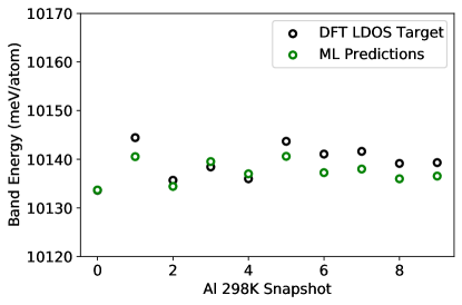
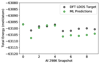
In Table 4 and Figure 8, we demonstrate that the 298 K model is able to achieve the highest and most consistent accuracy of all models considered in this work. Using a single training snapshot and a single validation snapshot, the ML-DFT model is able to achieve mean absolute band energy error of 2.48 meV/atom and mean absolute total energy error of 3.07 meV/atom. Furthermore, the 298 K model surpasses the 5 meV/atom accuracy for the most accurate ML-IAPs in large-scale MD simulations [102]. The low variability, seen in Figure 7, is more easily exploited by ML-DFT’s grid-based approach relative to the 933 K cases.
References
- Horstemeyer [2012] M. F. Horstemeyer, The near Future: ICME for the Creation of New Materials and Structures, in Integrated Computational Materials Engineering (ICME) for Metals (John Wiley & Sons, Ltd, 2012) Chap. 10, pp. 410–423.
- Frazier [2014] W. E. Frazier, Metal Additive Manufacturing: A Review, Journal of Materials Engineering and Performance 23, 1917 (2014).
- Antony and Davim [2018] K. Antony and J. P. Davim, eds., Advanced Manufacturing and Materials Science: Selected Extended Papers of ICAMMS 2018, Lecture Notes on Multidisciplinary Industrial Engineering (Springer International Publishing, 2018).
- Mao et al. [2003] W. L. Mao, H.-k. Mao, P. J. Eng, T. P. Trainor, M. Newville, C.-c. Kao, D. L. Heinz, J. Shu, Y. Meng, and R. J. Hemley, Bonding Changes in Compressed Superhard Graphite, Science 302, 425 (2003).
- Fried et al. [2001] L. E. Fried, M. R. Manaa, P. F. Pagoria, and R. L. Simpson, Design and Synthesis of Energetic Materials, Annual Review of Materials Research 31, 291 (2001).
- Pagoria et al. [2002] P. F. Pagoria, G. S. Lee, A. R. Mitchell, and R. D. Schmidt, A review of energetic materials synthesis, Thermochimica Acta ENERGETIC MATERIALS, 384, 187 (2002).
- Werner and Fahrner [2001] M. Werner and W. Fahrner, Review on materials, microsensors, systems and devices for high-temperature and harsh-environment applications, IEEE Transactions on Industrial Electronics 48, 249 (2001).
- Was [2007] G. S. Was, Fundamentals of Radiation Materials Science: Metals and Alloys (Springer-Verlag, Berlin Heidelberg, 2007).
- Graham et al. [1986] R. Graham, B. Morosin, E. Venturini, and M. Carr, Materials Modification and Synthesis Under High Pressure Shock Compression, Annual Review of Materials Science 16, 315 (1986).
- Sawaoka [1986] A. B. Sawaoka, The Role of Shock Wave Compression in Materials Science, in Shock Waves in Condensed Matter, edited by Y. M. Gupta (Springer US, Boston, MA, 1986) pp. 51–56.
- Alfè and Gillan [1998] D. Alfè and M. J. Gillan, First-principles calculation of transport coefficients, Phys. Rev. Lett. 81, 5161 (1998).
- Militzer et al. [2008] B. Militzer, W. B. Hubbard, J. Vorberger, I. Tamblyn, and S. A. Bonev, A massive core in jupiter predicted from first-principles simulations, The Astrophysical Journal 688, L45 (2008).
- Vorberger et al. [2007] J. Vorberger, I. Tamblyn, B. Militzer, and S. A. Bonev, Hydrogen-helium mixtures in the interiors of giant planets, Phys. Rev. B 75, 024206 (2007).
- Schöttler and Redmer [2018] M. Schöttler and R. Redmer, Ab initio calculation of the miscibility diagram for hydrogen-helium mixtures, Phys. Rev. Lett 120, 115703 (2018).
- Nettelmann et al. [2012] N. Nettelmann, A. Becker, B. Holst, and R. Redmer, Astrophys. J. 750, 52 (2012).
- Nettelmann et al. [2013] N. Nettelmann, R. Helled, J. Fortney, and R. Redmer, Planet. Space Sci. 77, 143 (2013).
- Lorenzen et al. [2009] W. Lorenzen, B. Holst, and R. Redmer, Phys. Rev. Lett. 102, 115701 (2009).
- Lorenzen et al. [2011] W. Lorenzen, B. Holst, and R. Redmer, Phys. Rev. B 84, 235109 (2011).
- Nettelmann et al. [2011] N. Nettelmann, J. J. Fortney, U. Kramm, and R. Redmer, Thermal evolution and structure models of the transiting super-earth gj 1214b, Astrophys. J. 733, 2 (2011).
- Kramm et al. [2012] U. Kramm, N. Nettelmann, J. J. Fortney, R. Neuhäuser, and R. Redmer, Constraining the interior of extrasolar giant planets with the tidal love number k2 using the example of hat-p-13b”, A & A 538, 8 (2012).
- Alder and Wainwright [1959] B. J. Alder and T. E. Wainwright, Studies in Molecular Dynamics. I. General Method, The Journal of Chemical Physics 31, 459 (1959).
- Plimpton [1995] S. Plimpton, Fast Parallel Algorithms for Short-Range Molecular Dynamics, Journal of Computational Physics 117, 1 (1995).
- Zepeda-Ruiz et al. [2017] L. A. Zepeda-Ruiz, A. Stukowski, T. Oppelstrup, and V. V. Bulatov, Probing the limits of metal plasticity with molecular dynamics simulations, Nature 550, 492 (2017).
- Finnis [2003] M. Finnis, Interatomic Forces in Condensed Matter (Oxford University Press, 2003).
- Huan et al. [2017] T. D. Huan, R. Batra, J. Chapman, S. Krishnan, L. Chen, and R. Ramprasad, A universal strategy for the creation of machine learning-based atomistic force fields, npj Computational Materials 3, 10.1038/s41524-017-0042-y (2017).
- Smith et al. [2017] J. S. Smith, O. Isayev, and A. E. Roitberg, Ani-1: an extensible neural network potential with dft accuracy at force field computational cost, Chem. Sci. 8, 3192 (2017).
- Zhang et al. [2018] L. Zhang, J. Han, H. Wang, R. Car, and W. E, Deep Potential Molecular Dynamics: A Scalable Model with the Accuracy of Quantum Mechanics, Phys. Rev. Lett. 120, 143001 (2018).
- Bartók et al. [2010a] A. P. Bartók, M. C. Payne, R. Kondor, and G. Csányi, Gaussian Approximation Potentials: The Accuracy of Quantum Mechanics, without the Electrons, Phys. Rev. Lett. 104, 136403 (2010a).
- Jaramillo-Botero et al. [2014] A. Jaramillo-Botero, S. Naserifar, and W. A. Goddard, General Multiobjective Force Field Optimization Framework, with Application to Reactive Force Fields for Silicon Carbide, Journal of Chemical Theory and Computation 10, 1426 (2014).
- Lubbers et al. [2018] N. Lubbers, J. S. Smith, and K. Barros, Hierarchical modeling of molecular energies using a deep neural network, The Journal of Chemical Physics 148, 241715 (2018).
- Schütt et al. [2018] K. T. Schütt, H. E. Sauceda, P.-J. Kindermans, A. Tkatchenko, and K.-R. Müller, SchNet – A deep learning architecture for molecules and materials, The Journal of Chemical Physics 148, 241722 (2018).
- Thompson et al. [2015a] A. P. Thompson, L. P. Swiler, C. R. Trott, S. M. Foiles, and G. J. Tucker, Spectral neighbor analysis method for automated generation of quantum-accurate interatomic potentials, Journal of Computational Physics 285, 316 (2015a).
- Hohenberg and Kohn [1964] P. Hohenberg and W. Kohn}Inhomogeneous Electron Gas, Phys. Rev. 136, B864 (1964).
- Kohn and Sham [1965] W. Kohn and L. J. Sham, Self-Consistent Equations Including Exchange and Correlation Effects, Phys. Rev. 140, A1133 (1965).
- Mermin [1965] N. D. Mermin, Thermal Properties of the Inhomogeneous Electron Gas, Physical Review 137, A1441 (1965).
- Burke [2012] K. Burke, Perspective on density functional theory, J. Chem. Phys. 136, 10.1063/1.4704546 (2012).
- Becke [2014] A. D. Becke, Perspective: Fifty years of density-functional theory in chemical physics, The Journal of Chemical Physics 140, 18A301 (2014).
- Lejaeghere et al. [2016] K. Lejaeghere, G. Bihlmayer, T. Björkman, P. Blaha, S. Blügel, V. Blum, D. Caliste, I. E. Castelli, S. J. Clark, A. D. Corso, S. de Gironcoli, T. Deutsch, J. K. Dewhurst, I. D. Marco, C. Draxl, M. Dułak, O. Eriksson, J. A. Flores-Livas, K. F. Garrity, L. Genovese, P. Giannozzi, M. Giantomassi, S. Goedecker, X. Gonze, O. Grånäs, E. K. U. Gross, A. Gulans, F. Gygi, D. R. Hamann, P. J. Hasnip, N. a. W. Holzwarth, D. Iuşan, D. B. Jochym, F. Jollet, D. Jones, G. Kresse, K. Koepernik, E. Küçükbenli, Y. O. Kvashnin, I. L. M. Locht, S. Lubeck, M. Marsman, N. Marzari, U. Nitzsche, L. Nordström, T. Ozaki, L. Paulatto, C. J. Pickard, W. Poelmans, M. I. J. Probert, K. Refson, M. Richter, G.-M. Rignanese, S. Saha, M. Scheffler, M. Schlipf, K. Schwarz, S. Sharma, F. Tavazza, P. Thunström, A. Tkatchenko, M. Torrent, D. Vanderbilt, M. J. van Setten, V. V. Speybroeck, J. M. Wills, J. R. Yates, G.-X. Zhang, and S. Cottenier, Reproducibility in density functional theory calculations of solids, Science 351, 10.1126/science.aad3000 (2016).
- Pribram-Jones et al. [2015] A. Pribram-Jones, D. A. Gross, and K. Burke, DFT: A Theory Full of Holes?, Annual Review of Physical Chemistry 66, 10.1146/annurev-physchem-040214-121420 (2015).
- Wood et al. [2019] M. A. Wood, M. A. Cusentino, B. D. Wirth, and A. P. Thompson, Data-driven material models for atomistic simulation, Phys. Rev. B 99, 184305 (2019).
- Weck et al. [2018] P. F. Weck, K. R. Cochrane, S. Root, J. M. D. Lane, L. Shulenburger, J. H. Carpenter, T. Sjostrom, T. R. Mattsson, and T. J. Vogler, Shock compression of strongly correlated oxides: A liquid-regime equation of state for cerium(IV) oxide, Phys. Rev. B 97, 125106 (2018).
- Hansen et al. [2015] K. Hansen, F. Biegler, R. Ramakrishnan, W. Pronobis, O. A. von Lilienfeld, K.-R. Müller, and A. Tkatchenko, Machine Learning Predictions of Molecular Properties: Accurate Many-Body Potentials and Nonlocality in Chemical Space, The Journal of Physical Chemistry Letters 6, 2326 (2015).
- Rupp et al. [2012a] M. Rupp, A. Tkatchenko, K.-R. Müller, and O. A. von Lilienfeld, Fast and Accurate Modeling of Molecular Atomization Energies with Machine Learning, Phys. Rev. Lett. 108, 058301 (2012a).
- Schütt et al. [2017] K. T. Schütt, F. Arbabzadah, S. Chmiela, K. R. Müller, and A. Tkatchenko, Quantum-chemical insights from deep tensor neural networks, Nature Communications 8, 10.1038/ncomms13890 (2017).
- Schütt et al. [2014] K. T. Schütt, H. Glawe, F. Brockherde, A. Sanna, K. R. Müller, and E. K. U. Gross, How to represent crystal structures for machine learning: Towards fast prediction of electronic properties, Phys. Rev. B 89, 205118 (2014).
- Li et al. [2016] L. Li, J. C. Snyder, I. M. Pelaschier, J. Huang, U.-N. Niranjan, P. Duncan, M. Rupp, K.-R. Müller, and K. Burke, Understanding machine-learned density functionals, International Journal of Quantum Chemistry 116, 819 (2016).
- Snyder et al. [2013] J. C. Snyder, M. Rupp, K. Hansen, L. Blooston, K.-R. Müller, and K. Burke, Orbital-free bond breaking via machine learning, The Journal of Chemical Physics 139, 224104 (2013).
- Snyder et al. [2012] J. C. Snyder, M. Rupp, K. Hansen, K.-R. Müller, and K. Burke, Finding Density Functionals with Machine Learning, Phys. Rev. Lett. 108, 253002 (2012).
- Yao and Parkhill [2016] K. Yao and J. Parkhill, Kinetic Energy of Hydrocarbons as a Function of Electron Density and Convolutional Neural Networks, Journal of Chemical Theory and Computation 12, 1139 (2016).
- Brockherde et al. [2017] F. Brockherde, L. Vogt, L. Li, M. E. Tuckerman, K. Burke, and K.-R. Müller, Bypassing the Kohn-Sham equations with machine learning, Nature Communications 8, 10.1038/s41467-017-00839-3 (2017).
- Broderick and Rajan [2011] S. R. Broderick and K. Rajan, Eigenvalue decomposition of spectral features in density of states curves, EPL (Europhysics Letters) 95, 57005 (2011).
- Ben Mahmoud et al. [2020] C. Ben Mahmoud, A. Anelli, G. Csányi, and M. Ceriotti, Learning the electronic density of states in condensed matter (2020), arXiv:2006.11803 [cond-mat.mtrl-sci] .
- Chandrasekaran et al. [2019] A. Chandrasekaran, D. Kamal, R. Batra, C. Kim, L. Chen, and R. Ramprasad, Solving the electronic structure problem with machine learning, npj Computational Materials 5, 10.1038/s41524-019-0162-7 (2019).
- Abedi et al. [2012] A. Abedi, N. T. Maitra, and E. K. U. Gross, Correlated electron-nuclear dynamics: Exact factorization of the molecular wavefunction, The Journal of Chemical Physics 137, 22A530 (2012).
- Grumbach et al. [1994] M. P. Grumbach, D. Hohl, R. M. Martin, and R. Car, Ab initio molecular dynamics with a finite-temperature density functional, Journal of Physics: Condensed Matter 6, 1999 (1994).
- Alavi et al. [1994] A. Alavi, J. Kohanoff, M. Parrinello, and D. Frenkel, Ab Initio Molecular Dynamics with Excited Electrons, Physical Review Letters 73, 2599 (1994).
- Alavi et al. [1995] A. Alavi, M. Parrinello, and D. Frenkel, Ab initio calculation of the sound velocity of dense hydrogen: Implications for models of Jupiter, Science 269, 1252 (1995).
- Marzari et al. [1997] N. Marzari, D. Vanderbilt, and M. C. Payne, Ensemble Density-Functional Theory for Ab Initio Molecular Dynamics of Metals and Finite-Temperature Insulators, Physical Review Letters 79, 1337 (1997).
- Alonso et al. [2010] J. L. Alonso, A. Castro, P. Echenique, V. Polo, A. Rubio, and D. Zueco, Ab Initio molecular dynamics on the electronic Boltzmann equilibrium distribution, New Journal of Physics 12, 083064 (2010).
- Abedi et al. [2010] A. Abedi, N. T. Maitra, and E. K. U. Gross, Exact factorization of the time-dependent electron-nuclear wave function, Phys. Rev. Lett. 105, 123002 (2010).
- Samanta et al. [2016] A. Samanta, M. A. Morales, and E. Schwegler, Exploring the free energy surface using ab initio molecular dynamics, The Journal of Chemical Physics 144, 164101 (2016).
- Toda et al. [1983] M. Toda, R. Kubo, and N. Saito, Statistical Physics I: Equilibrium Statistical Mechanics, Springer Series in Solid-State Sciences (Springer-Verlag, Berlin Heidelberg, 1983).
- Pittalis et al. [2011] S. Pittalis, C. R. Proetto, A. Floris, A. Sanna, C. Bersier, K. Burke, and E. K. U. Gross, Exact Conditions in Finite-Temperature Density-Functional Theory, Physical Review Letters 107, 163001 (2011).
- Baldsiefen et al. [2015] T. Baldsiefen, A. Cangi, and E. K. U. Gross, Reduced-density-matrix-functional theory at finite temperature: Theoretical foundations, Physical Review A 92, 052514 (2015).
- Pribram-Jones et al. [2014] A. Pribram-Jones, S. Pittalis, E. K. U. Gross, and K. Burke, Thermal Density Functional Theory in Context, in Frontiers and Challenges in Warm Dense Matter, Lecture Notes in Computational Science and Engineering, edited by F. Graziani, M. P. Desjarlais, R. Redmer, and S. B. Trickey (Springer International Publishing, Cham, 2014) pp. 25–60.
- Brown et al. [2013] E. W. Brown, J. L. DuBois, M. Holzmann, and D. M. Ceperley, Exchange-correlation energy for the three-dimensional homogeneous electron gas at arbitrary temperature, Physical Review B 88, 081102 (2013).
- Karasiev et al. [2014] V. V. Karasiev, T. Sjostrom, J. Dufty, and S. B. Trickey, Accurate Homogeneous Electron Gas Exchange-Correlation Free Energy for Local Spin-Density Calculations, Physical Review Letters 112, 076403 (2014).
- Groth et al. [2017] S. Groth, T. Dornheim, T. Sjostrom, F. D. Malone, W. M. C. Foulkes, and M. Bonitz, Ab initio Exchange-Correlation Free Energy of the Uniform Electron Gas at Warm Dense Matter Conditions, Physical Review Letters 119, 135001 (2017).
- Blöchl and Parrinello [1992] P. E. Blöchl and M. Parrinello, Adiabaticity in first-principles molecular dynamics, Physical Review B 45, 9413 (1992).
- Galli et al. [1990] G. Galli, R. M. Martin, R. Car, and M. Parrinello, Ab initio calculation of properties of carbon in the amorphous and liquid states, Physical Review B 42, 7470 (1990).
- Dreizler and Gross [1990] R. M. Dreizler and E. K. U. Gross, Density Functional Theory (Springer Berlin Heidelberg, 1990).
- Behler and Parrinello [2007a] J. Behler and M. Parrinello, Generalized Neural-Network Representation of High-Dimensional Potential-Energy Surfaces, Physical Review Letters 98, 146401 (2007a).
- Seko et al. [2014] A. Seko, A. Takahashi, and I. Tanaka, Sparse representation for a potential energy surface, Physical Review B 90, 024101 (2014).
- Snyder et al. [2015] J. C. Snyder, M. Rupp, K.-R. Müller, and K. Burke, Nonlinear gradient denoising: Finding accurate extrema from inaccurate functional derivatives, International Journal of Quantum Chemistry 115, 1102 (2015).
- Li et al. [2015] Z. Li, J. R. Kermode, and A. De Vita, Molecular Dynamics with On-the-Fly Machine Learning of Quantum-Mechanical Forces, Physical Review Letters 114, 096405 (2015).
- Giannozzi et al. [2009] P. Giannozzi, S. Baroni, N. Bonini, M. Calandra, R. Car, C. Cavazzoni, D. Ceresoli, G. L. Chiarotti, M. Cococcioni, I. Dabo, A. D. Corso, S. de Gironcoli, S. Fabris, G. Fratesi, R. Gebauer, U. Gerstmann, C. Gougoussis, A. Kokalj, M. Lazzeri, L. Martin-Samos, N. Marzari, F. Mauri, R. Mazzarello, S. Paolini, A. Pasquarello, L. Paulatto, C. Sbraccia, S. Scandolo, G. Sclauzero, A. P. Seitsonen, A. Smogunov, P. Umari, and R. M. Wentzcovitch, QUANTUM ESPRESSO: A modular and open-source software project for quantum simulations of materials, Journal of Physics: Condensed Matter 21, 395502 (2009).
- Giannozzi et al. [2017] P. Giannozzi, O. Andreussi, T. Brumme, O. Bunau, M. B. Nardelli, M. Calandra, R. Car, C. Cavazzoni, D. Ceresoli, M. Cococcioni, N. Colonna, I. Carnimeo, A. D. Corso, S. de Gironcoli, P. Delugas, R. A. DiStasio, A. Ferretti, A. Floris, G. Fratesi, G. Fugallo, R. Gebauer, U. Gerstmann, F. Giustino, T. Gorni, J. Jia, M. Kawamura, H.-Y. Ko, A. Kokalj, E. Küçükbenli, M. Lazzeri, M. Marsili, N. Marzari, F. Mauri, N. L. Nguyen, H.-V. Nguyen, A. Otero-de-la-Roza, L. Paulatto, S. Poncé, D. Rocca, R. Sabatini, B. Santra, M. Schlipf, A. P. Seitsonen, A. Smogunov, I. Timrov, T. Thonhauser, P. Umari, N. Vast, X. Wu, and S. Baroni, Advanced capabilities for materials modelling with Quantum ESPRESSO, Journal of Physics: Condensed Matter 29, 465901 (2017).
- Giannozzi et al. [2020] P. Giannozzi, O. Baseggio, P. Bonfà, D. Brunato, R. Car, I. Carnimeo, C. Cavazzoni, S. de Gironcoli, P. Delugas, F. Ferrari Ruffino, A. Ferretti, N. Marzari, I. Timrov, A. Urru, and S. Baroni, Quantum ESPRESSO toward the exascale, The Journal of Chemical Physics 152, 154105 (2020).
- Hamann [2013] D. R. Hamann, Optimized norm-conserving Vanderbilt pseudopotentials, Physical Review B 88, 085117 (2013).
- Perdew et al. [2008] J. P. Perdew, A. Ruzsinszky, G. I. Csonka, O. A. Vydrov, G. E. Scuseria, L. A. Constantin, X. Zhou, and K. Burke, Restoring the Density-Gradient Expansion for Exchange in Solids and Surfaces, Physical Review Letters 100, 136406 (2008).
- Monkhorst and Pack [1976] H. J. Monkhorst and J. D. Pack, Special points for Brillouin-zone integrations, Physical Review B 13, 5188 (1976).
- Hove [1953] L. V. Hove, The occurrence of singularities in the elastic frequency distribution of a crystal, Phys. Rev. 89, 1189 (1953).
- Blöchl et al. [1994] P. E. Blöchl, O. Jepsen, and O. K. Andersen, Improved tetrahedron method for Brillouin-zone integrations, Physical Review B 49, 16223 (1994).
- Rupp et al. [2012b] M. Rupp, A. Tkatchenko, K.-R. Müller, and O. A. von Lilienfeld, Fast and accurate modeling of molecular atomization energies with machine learning, Phys. Rev. Lett. 108, 058301 (2012b).
- Drautz [2019] R. Drautz, Atomic cluster expansion for accurate and transferable interatomic potentials, Physical Review B 99, 014104 (2019).
- Behler and Parrinello [2007b] J. Behler and M. Parrinello, Generalized neural-network representation of high-dimensional potential-energy surfaces, Physical review letters 98, 146401 (2007b).
- Bartók et al. [2010b] A. P. Bartók, M. C. Payne, R. Kondor, and G. Csányi, Gaussian approximation potentials: The accuracy of quantum mechanics, without the electrons, Physical review letters 104, 136403 (2010b).
- Thompson et al. [2015b] A. P. Thompson, L. P. Swiler, C. R. Trott, S. M. Foiles, and G. J. Tucker, Spectral neighbor analysis method for automated generation of quantum-accurate interatomic potentials, Journal of Computational Physics 285, 316 (2015b).
- Schmidt et al. [2019] J. Schmidt, M. R. Marques, S. Botti, and M. A. Marques, Recent advances and applications of machine learning in solid-state materials science, npj Computational Materials 5, 1 (2019).
- Mathuriya et al. [2018] A. Mathuriya, D. Bard, P. Mendygral, L. Meadows, J. Arnemann, L. Shao, S. He, T. Kärnä, D. Moise, S. J. Pennycook, K. Maschhoff, J. Sewall, N. Kumar, S. Ho, M. F. Ringenburg, Prabhat, and V. Lee, Cosmoflow: Using deep learning to learn the universe at scale, in Proceedings of the International Conference for High Performance Computing, Networking, Storage, and Analysis, SC ’18 (IEEE Press, 2018).
- He et al. [2016] K. He, X. Zhang, S. Ren, and J. Sun, Deep residual learning for image recognition, in IEEE CVPR (2016) pp. 770–778.
- Ziletti et al. [2018] A. Ziletti, D. Kumar, M. Scheffler, and L. Ghiringhelli, Insightful classification of crystal structures using deep learning, Nature Communications 9 (2018).
- Young et al. [2018] T. Young, D. Hazarika, S. Poria, and E. Cambria, Recent trends in deep learning based natural language processing [review article], IEEE Computational Intelligence Magazine 13, 55 (2018).
- Devlin et al. [2019] J. Devlin, M.-W. Chang, K. Lee, and K. Toutanova, BERT: Pre-training of deep bidirectional transformers for language understanding, in Proceedings of the 2019 Conference of the North American Chapter of the Association for Computational Linguistics: Human Language Technologies, Volume 1 (Long and Short Papers) (Association for Computational Linguistics, Minneapolis, Minnesota, 2019) pp. 4171–4186.
- Leshno et al. [1993] M. Leshno, V. Y. Lin, A. Pinkus, and S. Schocken, Multilayer feedforward networks with a nonpolynomial activation function can approximate any function, Neural Networks 6, 861 (1993).
- Goodfellow et al. [2016] I. Goodfellow, Y. Bengio, and A. Courville, Deep Learning (MIT Press, 2016) http://www.deeplearningbook.org.
- Prechelt [1996] L. Prechelt, Early stopping-but when?, in Neural Networks: Tricks of the Trade (1996).
- Lewis et al. [2000] R. M. Lewis, V. Torczon, and M. W. Trosset, Direct search methods: then and now, Journal of Computational and Applied Mathematics 124, 191 (2000), numerical Analysis 2000. Vol. IV: Optimization and Nonlinear Equations.
- Paszke et al. [2017] A. Paszke, S. Gross, S. Chintala, G. Chanan, E. Yang, Z. DeVito, Z. Lin, A. Desmaison, L. Antiga, and A. Lerer, Automatic differentiation in pytorch, NIPS (2017).
- Oliphant [2006] T. E. Oliphant, A guide to NumPy, Vol. 1 (Trelgol Publishing USA, 2006).
- Sergeev and Balso [2018] A. Sergeev and M. D. Balso, Horovod: fast and easy distributed deep learning in TensorFlow, arXiv preprint arXiv:1802.05799 (2018).
- Zuo et al. [2020] Y. Zuo, C. Chen, X. Li, Z. Deng, Y. Chen, J. Behler, G. Csanyi, A. V. Shapeev, A. P. Thompson, M. A. W̃ood, and S. P. Ong, Performance and cost assessment of machine learning interatomic potentials, J. Phys. Chem. A 124, 731 (2020).
- Pedregosa et al. [2011] F. Pedregosa, G. Varoquaux, A. Gramfort, V. Michel, B. Thirion, O. Grisel, M. Blondel, P. Prettenhofer, R. Weiss, V. Dubourg, J. Vanderplas, A. Passos, D. Cournapeau, M. Brucher, M. Perrot, and E. Duchesnay, Scikit-learn: Machine learning in Python, Journal of Machine Learning Research 12, 2825 (2011).