Abstract

Training of large scale models on distributed clusters is a critical component of the machine learning pipeline. However, this training can easily be made to fail if some workers behave in an adversarial (Byzantine) fashion whereby they return arbitrary results to the parameter server (PS). A plethora of existing papers consider a variety of attack models and propose robust aggregation and/or computational redundancy to alleviate the effects of these attacks. In this work we consider an omniscient attack model where the adversary has full knowledge about the gradient computation assignments of the workers and can choose to attack (up to) any $q$ out of $K$ worker nodes to induce maximal damage. Our redundancy-based method ByzShield leverages the properties of bipartite expander graphs for the assignment of tasks to workers; this helps to effectively mitigate the effect of the Byzantine behavior. Specifically, we demonstrate an upper bound on the worst case fraction of corrupted gradients based on the eigenvalues of our constructions which are based on mutually orthogonal Latin squares and Ramanujan graphs. Our numerical experiments indicate over a 36% reduction on average in the fraction of corrupted gradients compared to the state of the art. Likewise, our experiments on training followed by image classification on the CIFAR-10 dataset show that ByzShield has on average a 20% advantage in accuracy under the most sophisticated attacks. ByzShield also tolerates a much larger fraction of adversarial nodes compared to prior work.

1 Introduction

The explosive growth of machine learning applications have necessitated the routine training of large scale ML models in a variety of domains. Owing to computational and space constraints this training is typically run on distributed clusters. A common architecture consists of a single central server (parameter server or PS) which maintains a global copy of the model and several worker machines. The workers compute gradients of the loss function with respect to the parameters being optimized. The results are returned to the PS which aggregates them and updates the model. A new copy of the model is broadcasted from the PS to the workers and the above procedure is repeated until convergence. TensorFlow Abadi et al. (2016), MXNet Chen et al. (2015), CNTK Seide & Agarwal (2016) and PyTorch Paszke et al. (2019) are all examples of this architecture.

A major challenge with such setups as they scale is the fact that the system is vulnerable to adversarial attacks by the computing nodes (i.e., Byzantine behavior), or by failures/crashes thereof. As a result, the corresponding gradients returned to the PS are potentially unreliable for use in training and model updates. Achieving robustness in the face of Byzantine node behavior (which can cause gradient-based methods to converge slowly or to diverge) is of crucial importance and has attracted significant attention Gunawi et al. (2018); Dean et al. (2012); Kotla et al. (2007).

One class of methods investigates techniques for suitably aggregating the results from the workers. Blanchard et al. (2017) establishes that no linear aggregation method (such as averaging) can be robust even to a single faulty worker. Robust aggregation has been proposed as an alternative. Majority voting, geometric median and squared-distance-based techniques fall into this category Damaskinos et al. (2019); Yin et al. (2019; 2018); Xie et al. (2018); Blanchard et al. (2017); Chen et al. (2017). The benefit of such approaches is their robustness guarantees. However, they have serious weaknesses. First, they are very limited in terms of the fraction of Byzantine nodes they can withstand. Moreover, their complexity often scales quadratically with the number of workers Xie et al. (2018). Finally, their theoretical guarantees are insufficient to establish convergence and require strict assumptions such as convexity of the loss function.

Another category of defenses is based on redundancy and seeks resilience to Byzantines by replicating the gradient computations such that each of them is processed by more than one machine Yu et al. (2019); Rajput et al. (2019); Chen et al. (2018); Data et al. (2018). Even though this approach requires more computation load, it comes with stronger guarantees of correcting the erroneous gradients. Existing techniques are sometimes combined with robust aggregation Rajput et al. (2019). The main drawback of recent work in this category is that the training can be easily disrupted by a powerful omniscient adversary who has full control of a subset of the nodes and can mount judicious attacks.

1.1 Contributions

In this work, we propose our redundancy-based method ByzShield that provides robustness in the face of a significantly stronger attack model than has been considered in prior work. In particular, we consider an omniscient adversary who has full knowledge of the tasks assigned to the workers. The adversary is allowed to pick any subset of $q$ worker nodes to attack at each iteration of the algorithm. Our model allows for collusion among the Byzantine workers to inflict maximum damage on the training process.

Our work demonstrates an interesting link between achieving robustness and spectral graph theory. We show that using optimal expander graphs (constructed from mutually orthogonal Latin squares and Ramanujan graphs) allows us to assign redundant tasks to workers in such a way that the adversary’s ability to corrupt the gradients is significantly reduced as compared to the prior state of the art.

Our theoretical analysis shows that our method achieves a much lower fraction of corrupted gradients compared to other methods Rajput et al. (2019); this is supported by numerical simulations which indicate over a 36% reduction on average in the fraction of corrupted gradients. Our experimental results on large scale training for image classification (CIFAR-10) show that ByzShield has on average a 20% advantage in accuracy under the most sophisticated attacks.

Finally, we demonstrate the fragility of existing schemes Rajput et al. (2019) to simple attacks under our attack model when the number of Byzantine workers is large. In these cases, prior methods either diverge or are not applicable Damaskinos et al. (2019); Rajput et al. (2019); El Mhamdi et al. (2018), whereas ByzShield converges to high accuracy.

1.2 Related Work

Prior work in this area considers adversaries with a wide range of powers. For instance, DETOX and DRACO consider adversaries that are only able to attack a random set of workers. In our case, an adversary possesses full knowledge of the task assignment and attacked workers can collude. Prior work which considers the same adversarial model as ours includes Baruch et al. (2019); Xie et al. (2018); Yin et al. (2018); El Mhamdi et al. (2018); Shen et al. (2016) .

One of the most popular robust aggregation techniques is known as mean-around-median or trimmed mean Xie et al. (2018); Yin et al. (2018); El Mhamdi et al. (2018). It handles each dimension of the gradient separately and returns the average of a subset of the values that are closest to the median. Auror introduced in Shen et al. (2016) is a variant of trimmed median which partitions the values of each dimension into two clusters using k-means and discards the smaller cluster if the distance between the two exceeds a threshold; the values of the larger cluster are then averaged. signSGD in Bernstein et al. (2019) transmits only the sign of the gradient vectors from the workers to the PS and exploits majority voting to decide the overall update; this practice improves communication time and denies any individual worker too much effect on the update.

Krum in Blanchard et al. (2017) chooses a single honest worker for the next model update. The chosen gradient is the one closest to its $k\in\mathbb{N}$ nearest neighbors. The authors recognized in later work El Mhamdi et al. (2018) that Krum may converge to an ineffectual model in the landscape of non-convex high dimensional problems. They showed that a large adversarial change to a single parameter with a minor impact on the $L^{p}$ norm can make the model ineffective. They present an alternative defense called Bulyan to oppose such attacks. Nevertheless, if $K$ machines are used, Bulyan is designed to defend only up to $(K-3)/4$ fraction of corrupted workers. Similarly, the method of Chen et al. (2017) is based on the geometric median of means.

In the area of redundancy-based methods, DRACO in Chen et al. (2018) uses a simple Fractional Repetition Code (FRC) (that operates by grouping workers) and the cyclic repetition code introduced in Raviv et al. (2018); Tandon et al. (2017) to ensure robustness; majority vote and Fourier decoders try to alleviate the adversarial effects. Their work ensures exact recovery (as if the system had no adversaries) with $q$ Byzantine nodes, when each task is replicated $r\geq 2q+1$ times; the bound is information-theoretic minimum and DRACO is not applicable if it is violated. Nonetheless, this requirement is very restrictive for the typical assumption that up to half of the workers can be Byzantine.

DETOX in Rajput et al. (2019) extends the work of Chen et al. (2018) and uses a simple grouping strategy to assign the gradients. It performs multiple stages of aggregation to gradually filter the adversarial values. The first stage involves majority voting while the following stages perform robust aggregation, as discussed before. Unlike DRACO, the authors do not seek exact recovery hence the minimum requirement in $r$ is small. However, the theoretical resilience guarantees that DETOX provides depend heavily on a “random assignment” of tasks to workers and on “random choice” of the adversarial workers. Furthermore, their theoretical results hold when the fraction of Byzantines is less than $1/40$. Under these assumptions, they show that on average a small percentage of the gradient computations will be distorted.

2 Parallel Training Formulation

The formulation we discuss is standard in distributed deep learning. Assume that the loss function of the $i$-th sample is $l_{i}(\mathbf{w})$, where $\mathbf{w}\in\mathbb{R}^{d}$ is the parameter set of the model. We seek to minimize the empirical risk of the dataset, i.e.,

$$\min_{\mathbf{w}}L(\mathbf{w})=\min_{\mathbf{w}}\frac{1}{n}\sum\limits_{i=1}^{n}l_{i}(\mathbf{w})$$

where $n$ is the size of the dataset. This is typically solved iteratively via mini-batch Stochastic Gradient Descent (SGD) over distributed clusters. Initially, the parameters $\mathbf{w}$ are randomly set to $\mathbf{w}_{0}$ (in general, we will denote the state of the model at the end of iteration $t$ with $\mathbf{w}_{t}$). Following this, a randomly chosen batch $B_{t}$ of $b$ samples is used to perform the update in the $t$-th iteration. Thus,

$$\mathbf{w}_{t+1}=\mathbf{w}_{t}-\eta_{t}\frac{1}{|B_{t}|}\sum\limits_{i\in B_{t}}\nabla l_{i}(\mathbf{w}_{t})$$ (1)

where $\eta_{t}$ denotes the learning rate of the $t$-th iteration. In this work, we focus on synchronous SGD in which the PS waits for all workers to return before performing an update.

Within the cluster of $K+1$ servers the PS updates the global model after receiving computations from the workers. It also stores the dataset and the model and coordinates the protocol. The remaining servers, denoted $U_{0},\dots,U_{K-1}$, are the workers computing gradients on subsets of the batch.

Worker Assignment: A given batch $B_{t}$ is split into $f$ disjoint sets (or files) denoted $B_{t,i}$, for $i=0,\dots,f-1$. These files are then assigned to the workers according to a bipartite graph $\mathbf{G}=(\mathcal{U}\cup\mathcal{F}_{t},\mathcal{E})$, where $\mathcal{U}=\{U_{0},U_{1}\dots,U_{K-1}\}$ and $\mathcal{F}_{t}=\left\{B_{t,i}:i=0,1,\dots,f-1\right\}$ denote the workers and the files, respectively. An edge exists between $u\in\mathcal{U}$ and $v\in\mathcal{F}_{t}$ if worker $u$ is assigned file $v$. Any given file is assigned to $r>1$ workers ($r$ is called the replication factor); this allows for protection against Byzantine behavior. It follows that each worker is responsible for $l=fr/K$ files; $l$ is called the computational load. We let $\mathcal{N}(S)$ denote the set of neighbors of a subset $S$ of the nodes. Thus, $\mathcal{N}(U_{j})$ is the set of files assigned to worker $U_{j}$ and $\mathcal{N}(B_{t,i})$ is the set of workers that are assigned file $B_{t,i}$.

Byzantine Attack Model: We consider a model where $q$ workers operate in a Byzantine fashion, i.e., they can return arbitrary values to the PS. Our attack setup is omniscient where every worker knows the data assignment of all other participants and the model at every iteration; the choice of the Byzantine workers can also change across iterations. Furthermore, the Byzantine machines can collude to induce maximal damage. We will suppose that the fraction of Byzantine workers $\epsilon=q/K$ is less than $1/2$. We emphasize that this is a stronger adversary model than those considered in other redundancy-based work Rajput et al. (2019); Chen et al. (2018). Let $\hat{\mathbf{g}}_{t,i}^{(j)}$ be the value returned from the $j$-th worker to the PS for assigned file $B_{t,i}$. Then,

$$\hat{\mathbf{g}}_{t,i}^{(j)}=\left\{\begin{array}[]{ll}\mathbf{g}_{t,i}&\text{ if }U_{j}\text{ is honest},\\ \mathbf{x}&\text{otherwise}\\ \end{array}\right.$$ (2)

where $\mathbf{g}_{t,i}$ is the sum of the loss gradients on all samples in file $B_{t,i}$, i.e.,

$$\mathbf{g}_{t,i}=\sum\limits_{j\in B_{t,i}}\nabla l_{j}(\mathbf{w}_{t})$$

and $\mathbf{x}$ is any arbitrary vector in $\mathbb{R}^{d}$.

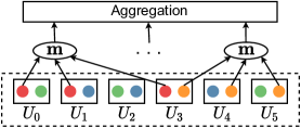
Figure 1: Aggregation of gradients on a training cluster.

Training Protocol: The training protocol followed in our work is similar to the one introduced in Rajput et al. (2019). Following the assignment of files, each worker $U_{j}$ computes the gradients of the samples in $\mathcal{N}(U_{j})$ and sends them to the PS. Subsequently, the PS will perform a majority vote across the computations of each file. Recall that each file has been processed by $r$ workers. For each such file $B_{t,i}$, the PS decides a majority value $\mathbf{m}_{i}$

$$\mathbf{m}_{i}\stackrel{{\scriptstyle\mathclap{\mbox{def}}}}{{=}}\mathrm{majority}\left\{\hat{\mathbf{g}}_{t,i}^{(j)}:U_{j}\in\mathcal{N}(B_{t,i})\right\}.$$ (3)

In our implementation, the majority function picks out the gradient that appears the maximum number of times. We ensure that there are no floating point precision issues with this method, i.e., all honest workers assigned to $B_{t,i}$ will return the exact same gradient. However, potential precision issues can easily be handled by deciding the majority by defining appropriate clusters amongst the returned gradients.

Assume that $r$ is odd (needed in order to avoid breaking ties) and let $r^{\prime}=\frac{r+1}{2}$. Under the majority rule in Eq. (3), the gradient on a file is distorted only if at least $r^{\prime}$ of the computations are performed by Byzantine workers. Following the majority vote, the gradients go through an aggregation step. One demonstration of this procedure is in Figure 1. There are $K=6$ machines and $f=4$ distinct files (represented by colored circles) replicated $r=3$ times. Each of the workers is assigned to two files and computes the sum of gradients (or an adversarial vector) on each file. At the next step, all returned values for the red file will be evaluated by a majority vote function (“$\mathbf{m}$” ellipses) on the PS which decides a single output value; a similar voting is done for the other 3 files. After the majority voting process, the “winning” gradients $\mathbf{m}_{i}$, $i=0,1,\dots,f-1$ can be further filtered by some aggregation function; in ByzShield we chose to apply coordinate-wise median. The entire procedure is described in Algorithm 1.

Figures of Merit: Firstly, we consider (i) the fraction of the estimated gradients $\mathbf{m}_{i}$ which are potentially erroneous. However, the end goal is to understand how the presence of Byzantine workers affects the overall training of the model under the different schemes. Towards this end, we will also measure the (ii) accuracy of the trained model on classification tasks. Finally, robustness to adversaries comes at the cost of increased training time. Thus, our third metric is (iii) overall time taken to fit the model. Asymptotic complexity (iv) is briefly addressed in the Appendix Section A.1.

Input: Data set of $n$ samples, batch size $b$, computation load $l$, redundancy $r$,
number of files $f$, maximum iterations $T$, assignment graph $\mathbf{G}$.

1 The PS randomly initializes model’s parameters to $\mathbf{w}_{0}$.

2 for $t=1$ to $T$ do

3       PS chooses a random batch $B_{t}\subseteq\{1,2,\dots,n\}$ of $b$ samples, partitions it into files and assigns them to workers based on graph $\mathbf{G}$. It then transmits model $\mathbf{w}_{t}$ to all workers.

4       for each worker $U_{j}$ do

5             if $U_{j}$ is honest then

6                   for each file $i\in\mathcal{N}(U_{j})$ do

7                         $U_{j}$ computes the sum of gradients

$$\hat{\mathbf{g}}_{t,i}^{(j)}=\sum\limits_{k\in B_{t,i}}\nabla l_{k}(\mathbf{w}_{t}).$$

8                   end for

9                  

10            else

11                   $U_{j}$ constructs adversarial vectors

$$\hat{\mathbf{g}}_{t,i_{1}}^{(j)},\hat{\mathbf{g}}_{t,i_{2}}^{(j)},\dots,\hat{\mathbf{g}}_{t,i_{l}}^{(j)}.$$

12             end if

13            $U_{j}$ returns $\hat{\mathbf{g}}_{t,i_{1}}^{(j)},\hat{\mathbf{g}}_{t,i_{2}}^{(j)},\dots,\hat{\mathbf{g}}_{t,i_{l}}^{(j)}$ to the PS.

14       end for

15      for $i=0$ to $f-1$ do

16             PS determines the $r$ workers in $\mathcal{N}(B_{t,i})$ which have processed $B_{t,i}$ and computes

$$\mathbf{m}_{i}=\mathrm{majority}\left\{\hat{\mathbf{g}}_{t,i}^{(j)}:j\in\mathcal{N}(B_{t,i})\}\right\}.$$

17       end for

18       PS updates the model via

$$\mathbf{w}_{t+1}=\mathbf{w}_{t}-\eta_{t}\frac{1}{n}\sum\limits_{i=0}^{n-1}\mathbf{m}_{i}.$$

19 end for

Algorithm 1 Majority-based algorithm to alleviate Byzantine effects.

3 Expansion Properties of Bipartite Graphs and Byzantine Resilience

The central idea of our work is that concepts from spectral graph theory Chung (1997) can guide us in the design of the bipartite graph $\mathbf{G}$ that specifies the worker-file assignment. In particular, we demonstrate that the spectral properties of the biadjacency matrix of $\mathbf{G}$ are closely related to the underlying expansion of the graph and can in turn be related to the scheme’s robustness under the omniscient attack model.

A graph with good expansion is one where any small enough set of nodes is guaranteed to have a large number of neighbors. This implies that the Byzantine nodes together process a large number of files which in turn means that their ability to corrupt the majority on many of them is limited.

For a bipartite graph $\mathbf{G}=(V_{1}\cup V_{2},E)$ with $|V_{1}|=K,|V_{2}|=f$, its biadjacency matrix $H$ is defined as

$$H_{i,j}=\left\{\begin{array}[]{ll}1&\text{ if }(i,j)\in E,\\ 0&\text{otherwise.}\\ \end{array}\right.$$ (4)

We only consider biregular $\mathbf{G}$ where the left and right degrees of all nodes are the same; these are denoted $d_{L}$ and $d_{R}$ respectively. Let $A=\frac{1}{\sqrt{d_{L}d_{R}}}H$ denote the normalized biadjacency matrix. It is known that the eigenvalues of $AA^{T}$ (or $A^{T}A$) are $1=\mu_{0}>\mu_{1}\geq\cdots\geq\mu_{K-1}\geq\mu_{K}=\cdots=\mu_{f-1}=0$ if $K<f$ Chung (1997).

For a subset of the vertices $S$, let $\mathrm{vol}(S)$ denote the number of edges that connect a vertex in $S$ with another vertex not in $S$. We will use the following lemma Zhu & Chugg (2007).

Lemma 1.

For any bipartite graph $\mathbf{G}=(\mathcal{U}\cup\mathcal{F},\mathcal{E})$ and a subset $S$ of $\mathcal{U}$ (or $\mathcal{F}$)

$$\frac{\mathrm{vol}(\mathcal{N}(S))}{\mathrm{vol}(S)}\geq\frac{1}{\mu_{1}+(1-\mu_{1})\frac{\mathrm{vol}(S)}{|\mathcal{E}|}}.$$

Now suppose that the bipartite graph $\mathbf{G}$ chosen for the worker-file assignment has a second-eigenvalue = $\mu_{1}$. Based on Lemma 1, if $S$ is a set of $q$ Byzantine workers, then $\mathrm{vol}(S)=ql$ since $\mathbf{G}$ is bipartite. By substitution, we compute that the number of files collectively being processed by the workers in $S$ is lower bounded as follows.

$$|\mathcal{N}(S)|\geq\frac{ql/r}{\mu_{1}+(1-\mu_{1})\frac{q}{K}}\stackrel{{\scriptstyle\mathclap{\mbox{def}}}}{{=}}\beta.$$ (5)

Claim 1.

Let $c_{\mathrm{max}}^{(q)}$ be the maximum number of files one can distort with $q$ Byzantines (since there is a bijection between gradients and files distorting a file is equivalent to distorting the gradient of the samples it contains hence the two terms will be used interchangeably). Then,

$$c_{\mathrm{max}}^{(q)}\leq\frac{l|S|-\beta}{r^{\prime}-1}=\frac{ql-\beta}{(r-1)/2}\stackrel{{\scriptstyle\mathclap{\mbox{def}}}}{{=}}\gamma.$$

An interesting observation stemming from the above upper bound is that as $\beta$ increases (i.e., as a particular fixed-sized subset of workers collectively processes more files) the maximum number of file gradients they can distort is reduced.

4 Task Assignment

In this section, we propose two different techniques of constructing the graph $\mathbf{G}$ which determines the allocation of gradient tasks to workers in ByzShield. Our graphs have $|\mathcal{U}|\leq|\mathcal{F}|$ (i.e., fewer workers than files) and possess optimal expansion properties in terms of their spectrum.

4.1 Task Assignment Based on Latin Squares

We extensively use combinatorial structures known as Latin squares Van Lint & Wilson (2001) (in short, LS) in this protocol. These designs have been used extensively in error-correcting codes Milenkovic & Laendner (2004). The basic definitions and known results about them that we will need in our exposition are presented below.

Table 1: A set of three MOLS of degree $5$.

0	1	2	3	4
1	2	3	4	0
2	3	4	0	1
3	4	0	1	2
4	0	1	2	3

1(a) $L_{1}$

0	1	2	3	4
2	3	4	0	1
4	0	1	2	3
1	2	3	4	0
3	4	0	1	2

1(b) $L_{2}$

0	1	2	3	4
3	4	0	1	2
1	2	3	4	0
4	0	1	2	3
2	3	4	0	1

1(c) $L_{3}$

4.1.1 Basic Definitions and Properties

We begin with the definition of a Latin square.

Definition 1.

A Latin square of degree $l$ is a quadruple $(R,C,S;L)$ where $R,C$ and $S$ are sets with $l$ elements each and $L$ is a mapping $L:R\times C\rightarrow S$ such that for any $i\in R$ and $x\in S$, there is a unique $j\in C$ such that $L(i,j)=x$. Also, any two of $i\in R$, $j\in C$ and $x\in S$ uniquely determine the third so that $L(i,j)=x$.

We refer to the sets $R$, $C$ and $S$ as rows, columns and symbols of the Latin square, respectively. The representation of a LS is an $l\times l$ array $L$ where the cell $L_{ij}$ contains $L(i,j)$.

Definition 2.

Two Latin squares $L_{1}:R\times C\rightarrow S$ and $L_{2}:R\times C\rightarrow T$ (with the same row and column sets) are said to be orthogonal when for each ordered pair $(s,t)\in S\times T$, there is a unique cell $(i,j)\in R\times C$ so that $L_{1}(i,j)=s$ and $L_{2}(i,j)=t$.

A set of $k$ Latin squares of degree $l$ which are pairwise orthogonal are called mutually orthogonal or MOLS. It can be shown Van Lint & Wilson (2001) that the maximal size of an orthogonal set of Latin squares of degree $l$ is $l-1$.

We use a standard construction which yields $l-1$ MOLS of degree $l$. Initially, pick a prime power $l$. $(i)$ All row, column and symbol sets are to be the elements of $\mathbb{F}_{l}$ (the finite field of size $l$), i.e., $R=C=S=\mathbb{F}_{l}=\{0,1,\dots,l-1\}$. $(ii)$ Then, for each nonzero element $\alpha$ in $\mathbb{F}_{l}$, define $L_{\alpha}(i,j):=\alpha i+j$ (addition is over $\mathbb{F}_{l}$). The $l-1$ squares created in this manner are MOLS since linear equations of the form $ai+bj=s$, $ci+dj=t$ have unique solutions $(i,j)$ provided that $ad-bc\neq 0$ which is the case here.

Table 11(c) shows an example of the above procedure that yields four MOLS of degree $5$ (only the first three are shown and will be used in the sequel) for $R=C=S=\mathbb{F}_{5}=\{0,1,\dots,4\}$ and $L_{\alpha}(i,j)=\alpha i+j\ (\mathrm{mod}\ 5)$, $\alpha=1,2,3$.

Input: Batch size $b$, computation load $l$, redundancy $r\leq l-1$, empty graph $\mathbf{G}$ with worker vertices $\mathcal{U}$ and file vertices $\mathcal{F}_{t}$.

1 The PS partitions $B_{t}$ into $l^{2}$ disjoint files of $b/l^{2}$ samples each

$$B_{t}=\left\{B_{t,i}:i=0,1,\dots,l^{2}-1\right\}=\mathcal{F}_{t}.$$

2 The PS constructs a set of $r$ MOLS $L_{1},L_{2},\dots,L_{r}$ of degree $l$ with symbols $S=\{0,1,\dots,l-1\}$.

3 for $k=0$ to $r-1$ do

4       for $s=0$ to $l-1$ do

5             PS identifies all cells $(i,j)$ with symbol $s$ in $L_{k+1}$ and connects vertex (file) $B_{t,il+j}$ to vertex (worker) $U_{kl+s}$ in $\mathbf{G}$.

6       end for

7      

8 end for

9

Algorithm 2 Proposed MOLS-based assignment.

4.1.2 Redundant Task Allocation

To allocate the batch of an iteration, $B_{t}$, to workers, first, we will partition $B_{t}$ into $f=l^{2}$ disjoint files $B_{t,0},B_{t,2},\dots,B_{t,l^{2}-1}$ of $b/l^{2}$ samples each where $l$ is the degree of a set of MOLS constructed as in Sec. 4.1.1. Following this we construct a bipartite graph specifying the placement according to the MOLS (see Algorithm 2).

The following example showcases the proposed protocol of Algorithm 2 using the MOLS from Table 11(c).

Example 1.

Consider $K=15$ workers $U_{0},\dots,U_{14}$, $l=5$ and $r=3$. Based on our protocol the $l^{2}=25$ files of each batch $B_{t}$ would be arranged on a grid $L$, as defined above. Since $r=3$, the construction (see line 2 of the algorithm) involves the use of $3$ MOLS of degree $l=5$, shown in Table 11(c). For the LS $L_{1}$ ($k=0$ in step 2 of the algorithm) choose, e.g., symbol $s=0$. The locations of $s=0$ in $L_{1}$ are $(0,0),(1,4),(2,3),(3,2)\text{ and }(4,1)$ and the files in those cells in $L$ are $B_{t,0},B_{t,9},B_{t,13},B_{t,17}\text{ and }B_{t,21}.$ Hence, $U_{0}$ will receive those files from the PS. The complete file assignment for the cluster is shown in Table 22(c) (the index $i$ of file $B_{t,i}$ has been used instead for brevity).

It is evident that each worker stores $l$ files. Another observation that follows from the placement policy (cf. Algorithm 2) and Definition 1 is that any two workers populated based on the same Latin square do not share any files while Definition 2 implies that a pair of workers populated based on two orthogonal Latin squares should share exactly one file.

4.2 Task Assignment Based on Direct Graph Constructions

We next focus on direct construction of bipartite graphs for the task assignment. In this regard, we investigate Ramanujan bigraphs which have been shown to be optimal expanders Alon (1986). A formal definition follows.

Definition 3.

A $(d_{L},d_{R})$-biregular bipartite graph is a Ramanujan bigraph if the second largest singular value of its biadjacency matrix $H$ (from Eq. (4)) is less than or equal to $\sqrt{d_{L}-1}+\sqrt{d_{R}-1}$.

Equivalently, one can express the property in terms of the second largest eigenvalue of $AA^{T}$, as defined in Section 3. This equivalence will be discussed in Section 5 and in the corresponding proofs in the Appendix. Overall, we seek Ramanujan bigraphs which provably achieve the smallest possible value of the second largest eigenvalue of $AA^{T}$.

Table 2: File allocation for $l=5$, $r=3$ based on MOLS.

Node	Stores
$U_{0}$	$0,9,13,17,21$
$U_{1}$	$1,5,14,18,22$
$U_{2}$	$2,6,10,19,23$
$U_{3}$	$3,7,11,15,24$
$U_{4}$	$4,8,12,16,20$

2(a) 1st replica.

Node	Stores
$U_{5}$	$0,8,11,19,22$
$U_{6}$	$1,9,12,15,23$
$U_{7}$	$2,5,13,16,24$
$U_{8}$	$3,6,14,17,20$
$U_{9}$	$4,7,10,18,21$

2(b) 2nd replica.

Node	Stores
$U_{10}$	$0,7,14,16,23$
$U_{11}$	$1,8,10,17,24$
$U_{12}$	$2,9,11,18,20$
$U_{13}$	$3,5,12,19,21$
$U_{14}$	$4,6,13,15,22$

2(c) 3rd replica.

4.2.1 Redundant Task Allocation

There are many ways to construct a $(d_{L},d_{R})$-biregular bipartite graph with the Ramanujan property Høholdt & Janwa (2012); Sipser & Spielman (1996). We use the one presented in Burnwal et al. (2020). This method yields a $(s,m)$ or an $(m,s)$ biregular graph (depending on the relation between $m$ and $s$) for $m\geq 2$ and a prime $s$. It is based on LDPC “array code” matrices Fan (2001) and proceeds as follows.

• Step 1: Pick integer $m\geq 2$ and prime $s$.

• Step 2: Define a cyclic shift permutation matrix $P_{s\times s}$

  $$P_{ij}=\left\{\begin{array}[]{ll}1&\text{ if }j\equiv i-1\ (\mathrm{mod}\ s),\\ 0&\text{otherwise}\\ \end{array}\right.$$

  where $i=1,2,\dots,s$ and $j=1,2,\dots,s$.

• Step 3: Construct matrix $B$ as

  $$B=\begin{bmatrix}I_{s}&I_{s}&I_{s}&\cdots&I_{s}\\ I_{s}&P&P^{2}&\cdots&P^{m-1}\\ I_{s}&P^{2}&P^{4}&\cdots&P^{2(m-1)}\\ I_{s}&P^{3}&P^{6}&\cdots&P^{3(m-1)}\\ \vdots&\vdots&\vdots&\vdots&\vdots\\ I_{s}&P^{s-1}&P^{2(s-1)}&\cdots&P^{(m-1)(s-1)}\\ \end{bmatrix}.$$

  $B$ is a $s^{2}\times ms$ matrix constructed as a $s\times m$ block matrix. If $m\geq s$, then $H=B$ is chosen to be the biadjacency matrix of the bipartite graph, otherwise $H=B^{T}$ is chosen. In both cases, $H$ represents a Ramanujan bigraph. Note that $H$ is a zero-one biadjacency matrix since $P$ and hence all of its powers are permutation matrices.

As mentioned earlier, we will assume $K\leq f$. The rows of $H$ will therefore correspond to workers and the columns will correspond to files in both of the above cases. Since all blocks of $H$ are permutation matrices the support of each row (size of storage of worker) and column (replication of file) can be easily derived. This yields two cases when this construction is applied to our setup

$$(K,f,l,r)=\left\{\begin{array}[]{ll}(ms,s^{2},s,m)&\text{if }m<s,\\ (s^{2},ms,m,s)&\text{otherwise}.\end{array}\right.$$ (6)

We will refer to the case $m<s$ as Ramanujan Case 1 and to the other case as Ramanujan Case 2. We can have setups with identical parameters between the MOLS formulation and Case 1; specifically, one can choose the same computation load $l$ (for prime $l$) and replication factor $r$ such that $r<l$ which in both schemes will make use of $K=rl$ workers and $f=l^{2}$ files. The need for a prime $l$ makes the Ramanujan scheme less flexible in terms of choosing the computation load, though. Ramanujan Case 2 requires $r\geq l$ hence we examine this method separately.

In our schemes, we need to allocate $K$ workers such that $K$ factorizes as $K=rl$ or $K=r^{2}$, requiring a prime $l$, a prime power $l$ or a prime $r$. We argue that these conditions are not restrictive and many such choices of $K$ exist on modern distributed platforms such as Amazon EC2 few of which are presented in this paper.

5 Distortion Fraction Analysis

In this section, we perform a worst-case analysis of the fraction of distorted files (defined as $\hat{\epsilon}=c_{\mathrm{max}}^{(q)}/f$) incurred by various aggregation methods, including that of ByzShield.

A few reasons motivate this analysis. Our deep learning experiments (upcoming Section 6.2) show that $\hat{\epsilon}$ is a very useful indicator of the convergence of a model’s training. Also, this comparison shows the superiority of ByzShield in terms of theoretical robustness guarantees since we achieve a much smaller $\hat{\epsilon}$ for the same $q$. Finally, we demonstrate via numerical experiments that the quantity $\gamma$ is a tight upper bound on the exact value of $c_{\mathrm{max}}^{(q)}$ for ByzShield.

We next compute the spectrum of $AA^{T}$, as defined in Section 3, of our utilized constructions. The authors of Burnwal et al. (2020) [Theorem 6] have computed the set of singular values of $H$ of Ramanujan Cases 1 and 2. In order to have a direct comparison between the spectral properties of the MOLS scheme and these Ramanujan graphs, we have normalized $H$ and computed the eigenvalues of the corresponding $AA^{T}$ instead. For the MOLS scheme, the normalized biadjacency matrix $A$ has $d_{L}=l$ and $d_{R}=r$. We denote an eigenvalue $x$ with algebraic multiplicity $y$ with $(x,y)$. All proofs for this section are in the Appendix.

Lemma 2.

• MOLS and Ramanujan Case 1: $(AA^{T})_{MOLS}$ and $(AA^{T})_{Ram.1}$ require $2<r<l$ and have spectrum

  $$\{(1,1),(1/r,r(l-1)),(0,r-1)\}.$$

• Ramanujan Case 2: $(AA^{T})_{Ram.2}$ requires $r\leq l$, $r|l$ and has spectrum

  $$\{(1,1),(1/r,r(r-1)),(0,r-1)\}.$$

The eigenvalues are sorted in decreasing order of magnitude. Interestingly, $(AA^{T})_{Ram.1}$ has exactly the same spectrum as if the graph was constructed from a set of MOLS. Overall, the parameters $l,r$, number of workers $K=rl$, number of files $f=l^{2}$ and the second largest eigenvalue of $AA^{T}$, $\mu_{1}=1/r$, are all identical across the two schemes.

5.1 Upper Bounds of $\hat{\epsilon}^{ByzShield}$ Based on Graph Expansion

5.1.1 MOLS-based Graphs

Based on Lemma 2, $\mu_{1}=1/r$ is the second largest eigenvalue of $(AA^{T})_{MOLS}$. Substituting in the expression of Eq. (5), Claim 1 gives us the exact value for $\gamma$. It is a tight upper bound on $c_{\mathrm{max}}^{(q)}$ for the MOLS protocol and by normalizing it we conclude that an optimal attack with $q$ Byzantines, distorts a fraction of the files which is at most

$$\hat{\epsilon}^{MOLS}\leq\frac{\gamma}{f}=\frac{\frac{2q^{2}}{rl^{2}}}{1+(r-1)\frac{q}{rl}}.$$

5.1.2 Ramanujan Graphs

By Lemma 2, the underlying graph of the MOLS assignment is a Ramanujan graph and all results of Section 5.1.1 carry over verbatim to Case 1.

Case 2 needs to be treated separately since it leads to a different cluster setup with $K=s^{2}=r^{2}$ workers and $f=rl$ files with an underlying graph with $\mu_{1}=1/s=1/r$. A simple computation yields

$$\hat{\epsilon}^{Ram.2}\leq\frac{\gamma}{f}=\frac{\frac{2q^{2}}{r^{2}}}{r+(r-1)\frac{q}{r}}.$$

5.2 Exact Value of $\hat{\epsilon}^{ByzShield}$ in the Regime $q\leq r$

When $q\leq r$, i.e., in the regime where there are only a few Byzantine workers, we can provide exact values of $\hat{\epsilon}$ for our constructions. In particular we pick the $q$ workers to be Byzantine such that the multiset of the files stored collectively across them (also referred to as multiset sum) has the maximal possible number of files repeated at least $r^{\prime}$ times. In this way, the majority of the copies of those files is distorted and the aggregation produces erroneous gradients.

Claim 2.

The maximum distortion fraction incurred by an optimal attack for the regime $q\leq r$ is characterized as follows.

• If $r=3$, then $\hat{\epsilon}^{ByzShield}=\left\{\begin{array}[]{ll}0&\text{if }q<2,\\ 1/f&\text{if }q=2,\\ 3/f&\text{if }q=3.\end{array}\right.$

• If $r>3$, then $\hat{\epsilon}^{ByzShield}=\left\{\begin{array}[]{ll}0&\text{if }q<r^{\prime},\\ 1/f&\text{if }r^{\prime}\leq q<r,\\ 2/f&\text{if }q=r.\end{array}\right.$

5.3 Comparisons With Prior Work

We compare with the values of $\hat{\epsilon}$ achieved by baseline and other redundancy-based methods. Baseline approaches do not involve redundancy or majority voting; their aggregation is applied directly to the $K$ gradients returned by the workers and hence $f=K$ and $c_{\mathrm{max}}^{(q)}=q$ which yields a distortion fraction $\hat{\epsilon}=q/K$. We also compare the actual values of $c_{\mathrm{max}}^{(q)}$ for ByzShield against the theoretical upper bounds based on the expansion analysis in Section 5.1.

5.3.1 Achievable $\hat{\epsilon}$ of Prior Work Under Worst-case Attacks

We now present a direct comparison between our work and state-of-the-art schemes that are redundancy-based. DETOX in Rajput et al. (2019) and DRACO in Chen et al. (2018) both use the same Fractional Repetition Code (FRC) for the assignment and both use majority vote aggregation, hence we will treat them in a unified manner. Our goal is to establish that redundancy is not enough to achieve resilience to adversaries; rather, a careful task assignment is of major importance. The basic placement of FRC is splitting the $K$ workers into $K/r$ groups. Within a group, all workers are responsible for the same part of a batch of size $br/K$ and a majority vote aggregation is executed in the group. Their method fundamentally relies on the fact that the Byzantines are chosen at random for each iteration and hence the probability of at least $r^{\prime}$ Byzantines being in the same majority-vote group is low on expectation. However, in an omniscient setup, if an adversary chooses the Byzantines such that at least $r^{\prime}$ workers in each group are adversarial, then it is evident that all corresponding gradients will be distorted. Such an attack can distort the votes in $\lfloor\frac{q}{r^{\prime}}\rfloor$ groups. To formulate a direct comparison with ByzShield let us measure $\hat{\epsilon}$ in this worst-case scenario. For FRC, this is equal to the number of affected groups multiplied by the number of samples per group and normalized by $b$, i.e.,

$$\hat{\epsilon}^{FRC}=\frac{\lfloor\frac{q}{r^{\prime}}\rfloor\times br/K}{b}=\lfloor\frac{q}{r^{\prime}}\rfloor\times r/K.$$

We pinpoint that at the regime $q\leq r^{\prime}$ all of the aforementioned schemes, including ours, achieve perfect recovery since there are not enough adversaries to distort any file. In addition, DRACO would fail in the regime $q>r^{\prime}$ while ByzShield still demonstrates strong robustness results.

Table 3: Distortion fraction evaluation for MOLS-based assignment for $(K,f,l,r)=(15,25,5,3)$ and comparison.

$q$	$c_{\mathrm{max}}^{(q)}$	$\hat{\epsilon}^{ByzShield}$	$\hat{\epsilon}^{Baseline}$	$\hat{\epsilon}^{FRC}$	$\gamma$
$2$	1	0.04	0.13	0.2	2.11
$3$	3	0.12	0.2	0.2	4.29
$4$	5	0.2	0.27	0.4	6.96
$5$	8	0.32	0.33	0.4	10
$6$	12	0.48	0.4	0.6	13.33
$7$	14	0.56	0.47	0.6	16.9

5.3.2 Numerical Simulations

For ByzShield, we ran exhaustive simulations, i.e, we computed $c_{\mathrm{max}}^{(q)}$ considering all adversarial choices of $q$ out of $K$ workers. The evaluation of the MOLS-based allocation scheme of Section 4.1 for Example 1 with $(l,r)=(5,3)$ is in Table 3 where for different values of $q$ we report the simulated $c_{\mathrm{max}}^{(q)}$, the corresponding $\hat{\epsilon}$ and the upper bound $\gamma$. Since a Ramanujan-based scheme of Case 1 has the same properties, the upper bounds are expected to be identical (however the actual task assignment is in general different). An interesting observation is that the simulations of the actual value of $c_{\mathrm{max}}^{(q)}$ were also identical across the two; thus, both have been summarized in the same Table 3. More simulations including Ramanujan Case 2 are shown in Section A.5 of the Appendix. From these tables we deduce that $\gamma$ is a very accurate worst-case approximation of $c_{\mathrm{max}}^{(q)}$.

Comparing with the achieved $\hat{\epsilon}^{FRC}$ computed as in Section 5.3.1, note that ByzShield can tolerate a higher number of Byzantines while consistently maintaining a small fraction $\hat{\epsilon}$. In contrast, a worst-case attack on FRC raises this error very quickly with respect to $q$. On average, $\hat{\epsilon}^{ByzShield}=0.64\hat{\epsilon}^{FRC}$ in Table 3. Finally, ByzShield has a benefit over baseline methods for up to $q=5$ with respect to $\hat{\epsilon}$.

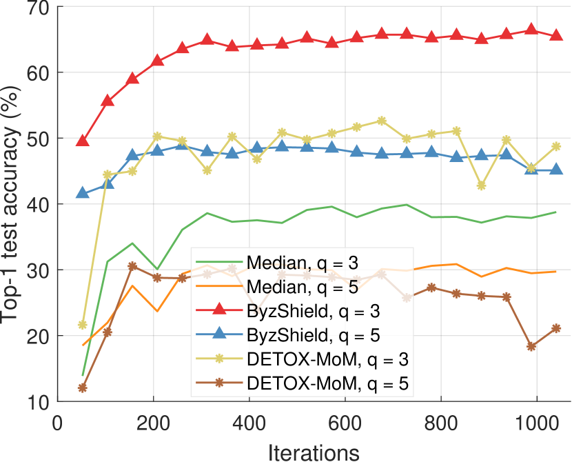
Figure 2: ALIE attack and median-based defenses (CIFAR-10).

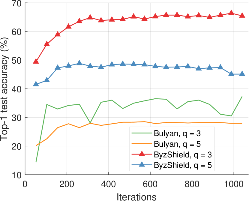
Figure 3: ALIE attack and Bulyan-based defenses (CIFAR-10).

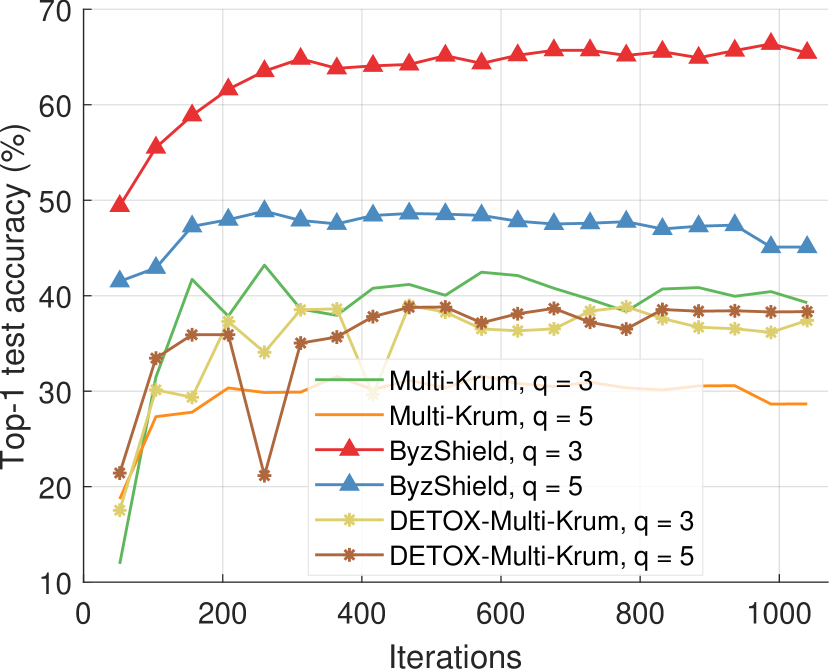
Figure 4: ALIE attack and Multi-Krum-based defenses (CIFAR-10).

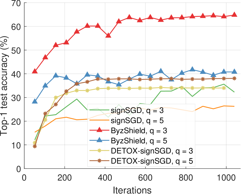
Figure 5: Constant attack and signSGD-based defenses (CIFAR-10).

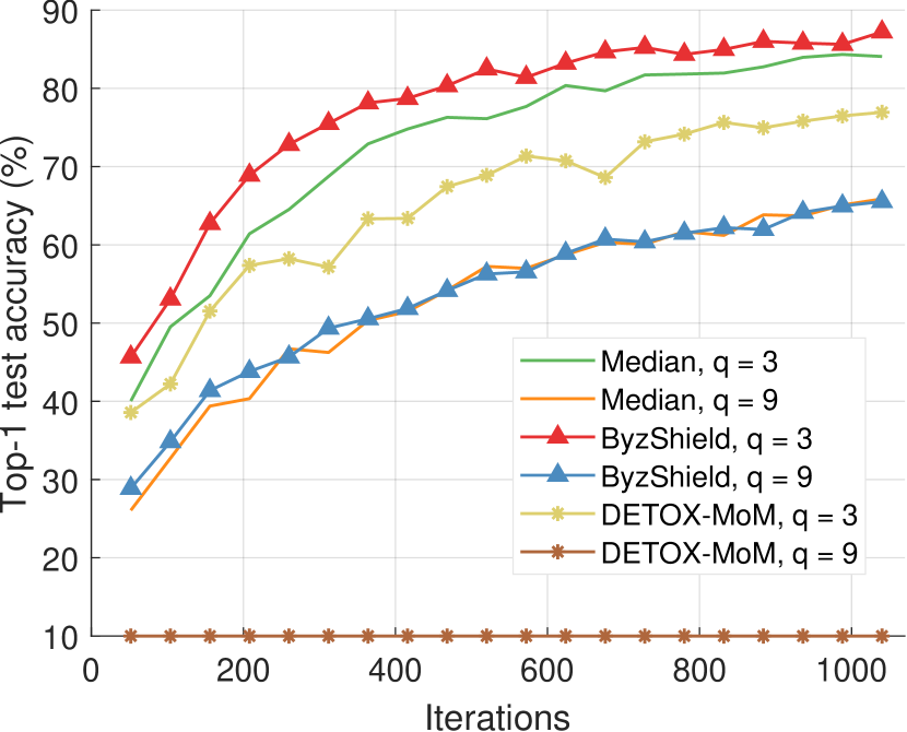
Figure 6: Reversed gradient attack and median-based defenses (CIFAR-10).

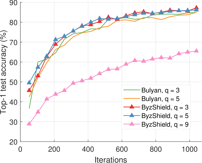
Figure 7: Reversed gradient attack and Bulyan-based defenses (CIFAR-10).

6 Large-scale Deep Learning Experiments

6.1 Experiment Setup

We have evaluated our method in classification tasks on large datasets on Amazon EC2 clusters. This project is written in PyTorch Paszke et al. (2019) and uses the MPICH library for communication among the devices. The implementation builds on DETOX’s skeleton and has been provided. The principal metric used in our evaluation is the top-1 test accuracy.

The classification tasks were performed using CIFAR-10 with ResNet-18 He et al. (2016). Experimenting with hyperparameter tuning we have chosen the values for batch size, learning rate scheduling, and momentum, among others. We used clusters of $K=25$ and $K=15$ workers of type c5.4xlarge on Amazon EC2 for various values of $q$. The PS was an i3.16xlarge instance in both cases. More details are in the Appendix.

The cluster of $K=25$ workers utilizes the Ramanujan Case 2 construction presented in Section 4.2.1 with $r=l=5$ resulting in partitioning each batch into $f=rl=25$ files. For $K=15$, we used the MOLS scheme (cf. Section 4.1) for $r=3$ and $l=5$ such that $f=l^{2}=25$. The corresponding simulated values of $c_{\mathrm{max}}^{(q)}$ and the fraction of distorted files, $\hat{\epsilon}$, under the attack on DETOX proposed in Section 5.3 are in Tables 4 and 3, respectively.

The attack models we tried are the following.

• ALIE Baruch et al. (2019): This attack involves communication among the Byzantines in which they jointly estimate the mean $\mu_{i}$ and standard deviation $\sigma_{i}$ of the batch’s gradient for each dimension $i$. They subsequently send a function of those moments to the PS such that it will distort the median of the results.

• Constant: Adversarial workers send a constant matrix with all elements equal to a fixed value; the matrix has the same dimensions as the true gradient.

• Reversed gradient: Byzantines return $-c\*g$ for $c>0$, to the PS instead of the true gradient $\*g$.

The ALIE algorithm is, to the best of our knowledge, the most sophisticated attack in literature for centralized setups. Our experiments showcase this fact. Constant attack often alters the gradients towards wrong directions in order to disrupt the model’s convergence and is also a powerful attack. Reversed gradient is the weakest among the three, as we will discuss in the Section 6.2.

We point out that in all of our experiments, we chose a set of $q$ Byzantines (among all $\binom{K}{q}$ possibilities) such that $\hat{\epsilon}$ is maximized; this is equivalent to a worst-case omniscient adversary which can control any $q$ devices.

The defense mechanism ByzShield applied on the outputs of the majority votes is coordinate-wise median Yin et al. (2019) across the $f$ gradients computed as in Algorithm 1 (lines 1-1). We decided to pair our method with median since in most cases it worked well and we did not have to resort to more sophisticated baseline defenses.

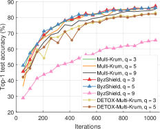
Figure 8: Reversed gradient attack and Multi-Krum-based defenses (CIFAR-10).

The most popular baseline techniques we compare against are median-of-means Minsker (2015), coordinate-wise majority voting with signSGD Bernstein et al. (2019), Multi-Krum Damaskinos et al. (2019) and Bulyan El Mhamdi et al. (2018). The latter two are robust to only a small fraction of erroneous results and their implementations rely on this assumption. Specifically, if $c_{\mathrm{max}}^{(q)}$ is the number of adversarial operands then Multi-Krum requires at least $2c_{\mathrm{max}}^{(q)}+3$ total number of operands while the same number for Bulyan is $4c_{\mathrm{max}}^{(q)}+3$. These constraints are very restrictive and the methods are inapplicable for larger values of $q$ for which our method is Byzantine-robust. DETOX Rajput et al. (2019) uses the aforementioned baseline methods for aggregating the “winning” gradients after the majority voting.

6.2 Results

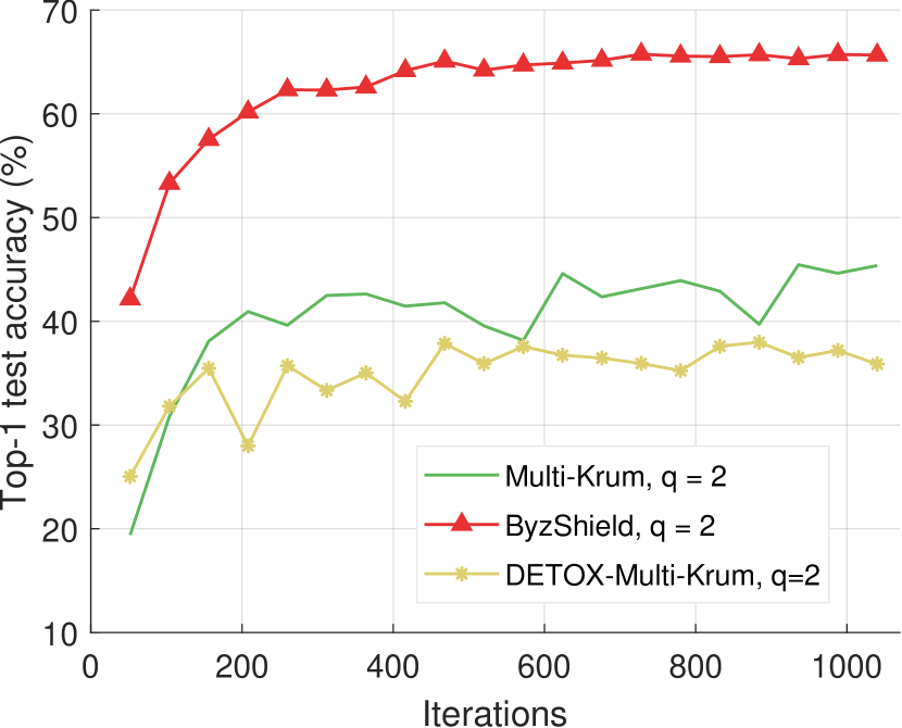
Figure 11: ALIE attack and Multi-Krum-based defenses (CIFAR-10), $K=15$.

In order to effectively interpret the results, the fraction of distorted gradients $\hat{\epsilon}$ needs to be taken into account; we will refer to the values in Appendix Table 4 throughout this exposition. Due to the nature of gradient-descent methods, $\hat{\epsilon}$ may not be always proportional to how well a method works but it is a good starting point. We will restrict our interpretation of the results to the case of $K=25$. For $K=15$, we performed a smaller range of experiments demonstrating similar effects (cf. Figures 11, 11, 11 in Appendix).

Let us focus on the results under the median-based defenses. In Figure 4, we compare ByzShield, the baseline implementation of coordinate-wise median ($\hat{\epsilon}=0.12,0.2$ for $q=3,5$, respectively) and DETOX with median-of-means ($\hat{\epsilon}=0.2$) under the ALIE attack. ByzShield achieves at least a 20% average accuracy overhead for both values of $q$ ($\hat{\epsilon}=0.04,0.08$ for $q=3,5$, respectively). In Figure 7 (reversed gradient), we observe similar trends. However, for $q=9$ in DETOX, a fraction of $\hat{\epsilon}=0.6$ majorities is distorted and even though this attack is considered weak, the method breaks (constant $10$% accuracy).

Similarly, ByzShield significantly outperforms Bulyan and Multi-Krum-based schemes on ALIE (Figures 4, 4); Bulyan cannot be paired with DETOX for $q\geq 1$ for our setup since the requirement $f\geq 4c_{\mathrm{max}}^{(q)}+3$, as discussed in Section 6.1, cannot be satisfied. The maximum allowed $q$ for DETOX with Multi-Krum (Figures 4 and 8) is $q=5$.

In signSGD, only the sign information of the gradient is retained and sent to the PS by the workers. The PS will output the majority of the signs for each dimension. The method’s authors Bernstein et al. (2019) suggest that gradient noise distributions are in principle unimodal and symmetric due to the Central Limit Theorem. Following the advice of Rajput et al. (2019), we pair this defense with the stronger constant attack as sign flips (e.g., reversed gradient) are unlikely to affect the gradient’s distribution. ByzShield with median still enjoys an accuracy improvement of about 20% for $q=3$ and a smaller one for $q=5$. The results are in Figure 7.

All schemes defend well under the reversed gradient attack for small values of $q$ (Figures 7, 7, 8). Nevertheless, in Figure 7, by testing ByzShield on large number of Byzantine workers ($q=9$) for which a fraction of $\hat{\epsilon}=0.36$ files are distorted, we realize that it still converges to a relatively high accuracy; Bulyan cannot be applied in this case. Multi-Krum has an advantage over our method for this attack for $q=9$ (Figure 8). DETOX cannot be paired with Multi-Krum in this case as it needs at least $2c_{\mathrm{max}}^{(q)}+3=7$ groups.

Note that in our adversarial scenario, DETOX may perform worse than its baseline counterpart depending on the fraction of corrupted gradients. For example, in Figure 7, for $q=3$, $\hat{\epsilon}^{DETOX}=0.2$ while $\hat{\epsilon}^{Median}=3/25=0.12$ and this reflects on better accuracy values for the baseline median.

There are two takeaways from these results. First, the distortion fraction $\hat{\epsilon}$ is a good predictor of an aggregation scheme’s convergence. Second, ByzShield supersedes prior schemes by an average of $20$% in terms of top-$1$ accuracy for large values of $q$ under various powerful attacks.

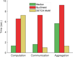
Figure 12: Per-iteration time estimate (ALIE attack and median-based defenses (CIFAR-10)).

Training Time: In ByzShield, within an iteration, a worker performs $l$ forward/backward propagations (one for each file) and transmits $l$ gradients back to the PS. The rest of the approaches have each worker return a single gradient. Hence, ByzShield spends more time on communication. In both DETOX and ByzShield a worker processes $r$ times more samples compared to a baseline technique. Thus, we expect redundancy-based methods to consume more time on computation at the worker level than their baseline counterparts. Aggregation time varies a lot by the method and the number of files to be processed by the PS for the model update. As an example, baseline median, ByzShield and DETOX median-of-means took 3.14, 10.81 and 4 hours, respectively, for the full training under the ALIE attack with $q=3$ (Figure 4). The corresponding per-iteration time (average across iterations) is in Figure 12 of the Appendix.

7 Conclusions and Future Work

We chose to utilize median for our method as it was performing well in all of our experiments. ByzShield can also be used with non-trivial aggregation schemes such as Bulyan and Multi-Krum and potentially yield even better results. Our scheme is significantly more robust than the most sophisticated defenses in literature at the expense of increased computation and communication time. We believe that implementation-related improvements such as adding support for GPUs can alleviate the overhead. Algorithmic improvements to make it more communication-efficient are also worth exploring. Finally, we considered an omniscient adversary and the worst-case choice of Byzantines. We think that this is a reasonable method if one wants to make fair and consistent comparisons across different schemes. But, weaker random attacks may also be an interesting direction.

Appendix A Appendix

A.1 Asymptotic Complexity

If the gradient computation has linear complexity and since each worker is assigned to $l$ files of $b/f$ samples each, the gradient computation cost at the worker level is $\mathcal{O}((lb/f)d)$ ($K$ such computations in parallel). In our schemes, however, $b$ is a constant multiple of $f$ and $l\leq r$; hence, the complexity becomes $\mathcal{O}(rd)$ which is identical to other redundancy-based schemes in Rajput et al. (2019); Chen et al. (2018). The complexity of aggregation varies significantly depending on the operator. For example, majority voting can be done in time which scales linearly with the number of votes using MJRTY proposed in Boyer & Moore (1991). In our case, this is $\mathcal{O}(Kd)$ as the PS needs to use the $d$-dimensional input from all $K$ machines. Krum Blanchard et al. (2017), Multi-Krum Damaskinos et al. (2019) and Bulyan El Mhamdi et al. (2018) are applied to all $K$ workers by default and require $\mathcal{O}(K^{2}(d+\mathrm{log}K))$.

A.2 Proof of Claim 1

Proof.

As all nodes in $S$ have degree $l$, the number of outgoing edges from $S$ is $l|S|$. For a file to be distorted it needs at least $r^{\prime}$ of its copies to be processed by Byzantine nodes. Furthermore, we know that collectively the nodes process at least $\beta$ files. Using these observations, we have

$$l|S|\geq c_{\mathrm{max}}^{(q)}r^{\prime}+(|\mathcal{N}(S)|-c_{\mathrm{max}}^{(q)})$$

$$\Rightarrow l|S|\geq c_{\mathrm{max}}^{(q)}r^{\prime}+(\beta-c_{\mathrm{max}}^{(q)})$$ (7)

$$\Rightarrow l|S|\geq c_{\mathrm{max}}^{(q)}(r^{\prime}-1)+\beta$$

$$\Rightarrow l|S|-\beta\geq c_{\mathrm{max}}^{(q)}(r^{\prime}-1)$$

$$\Rightarrow c_{\mathrm{max}}^{(q)}\leq\frac{l|S|-\beta}{r^{\prime}-1}=\frac{ql-\beta}{(r-1)/2}\stackrel{{\scriptstyle\mathclap{\mbox{def}}}}{{=}}\gamma$$

where in Eq. (7) we have substituted the result from Eq. (5). ∎

A.3 Proof of Lemma 2

Proof.

From Burnwal et al. (2020) [Theorem 6], the singular values of the zero-one (unnormalized) biadjacency matrix $H$ can be characterized in three distinct cases; we utilize the first two of them. They are presented below with the singular values reported in decreasing order of magnitude.

• Ramanujan Case 1: If $2\leq m<s$, then $H=B^{T}$ has singular values and corresponding multiplicities

  $$\{(\sqrt{sm},1),(\sqrt{s},m(s-1)),(0,m-1)\}.$$

• Ramanujan Case 2: If $m\geq s$ and $s|m$, then $H=B$ has singular values and corresponding multiplicities

  $$\{(\sqrt{sm},1),(\sqrt{m},(s-1)s),(0,s-1)\}.$$

In order to perform a direct comparison between the MOLS and Ramanujan construction we want to examine the eigenvalues of the normalized biadjacency matrix $A=\frac{1}{\sqrt{d_{L}d_{R}}}H$ (from Section 3) multiplied by its transpose, i.e., we are interested in the spectrum of $(AA^{T})_{Ram.1}$ and $(AA^{T})_{Ram.2}$. In all cases, observe that $d_{L}d_{R}=sm$ and the spectrum of $AA^{T}=\frac{1}{sm}HH^{T}$ in Lemma 2 of the main text is easily deduced; these eigenvalues will be the squares of the singular values of $H$ multiplied by $\frac{1}{sm}$.

We continue by computing the spectrum of $(AA^{T})_{MOLS}$. For a given Latin square $L$ we will use the term parallel class to denote the collection, i.e., the multiset consisting of the sets $\mathcal{N}(U_{i_{1}}),\mathcal{N}(U_{i_{2}}),\dots,\mathcal{N}(U_{i_{l}})$, where $U_{i_{1}},U_{i_{2}},\dots,U_{i_{l}}$ are the workers populated based on $L$. The classes for Latin squares $L_{1},\dots,L_{r}$ will be denoted with $\mathcal{P}_{1},\dots,\mathcal{P}_{r}$, respectively. The underlying principle is that a parallel class includes exactly one replica of each file. Let

$$X=l\left(\frac{1}{\sqrt{lr}}\right)^{2}I_{l}=\frac{1}{r}I_{l}=\left(\begin{array}[]{ccccc}1/r&&&&\makebox(0.0,0.0)[]{\text{0}}\\ &1/r&&&\\ &&\ddots&&\\ \makebox(0.0,0.0)[]{\text{0}}&&&&\\ &&&&1/r\\ \end{array}\right)$$

and

$$Y=1\left(\frac{1}{\sqrt{lr}}\right)^{2}J_{l}=\frac{1}{lr}J_{l}$$

where $J_{n}$ is the all-ones $n\times n$ matrix.

Based on the placement scheme introduced in Section 4.1.2 the matrix $(AA^{T})_{MOLS}$ takes the following $K\times K$ block form.

$$(AA^{T})_{MOLS}=\begin{bmatrix}X&Y&Y&\cdots&\cdots&Y\\ Y&X&Y&Y&\cdots&Y\\ Y&Y&X&Y&\ddots&\vdots\\ \vdots&\ddots&\ddots&\ddots&\ddots&Y\\ Y&\cdots&\cdots&Y&X&Y\\ Y&\cdots&\cdots&\cdots&Y&X\end{bmatrix}$$

Hence, the blocks of $(AA^{T})_{MOLS}$ take one of the forms $X,Y$. This is shown by observing that blocks $X$ concern multiplication of rows of $A$ with columns of $A^{T}$ which correspond to workers within a parallel class (if the index of the row of $A$ is the same as the index of the column of $A^{T}$ then $l$ entries $(\frac{1}{\sqrt{lr}})^{2}$ are added, otherwise there is no common file and the product is zero). Similarly, blocks that have the form of $Y$ concern pairs of workers from different parallel classes which share exactly one file.

We observe that

$$(AA^{T})_{MOLS}=\frac{1}{lr}\underbrace{\begin{pmatrix}0&1&\cdots&1\\ 1&0&\ddots&\vdots\\ \vdots&\ddots&\ddots&1\\ 1&\cdots&1&0\end{pmatrix}}_{=\ C_{r\times r}}\otimes J_{l}+\frac{1}{r}I_{lr}.$$ (8)

The characteristic polynomial of $J_{l}$ is $(\lambda-l)\lambda^{l-1}$ and its spectrum (with corresponding algebraic multiplicities) is $\sigma(J_{l})=\{(l,1),(0,l-1)\}$ Horn & Johnson (2012) which coincides with the spectrum of the adjacency matrix of a complete graph with self-edges.

Note 1.

If $\lambda$ is an eigenvalue of $A$ with eigenvector $\mathbf{x}$, then $\lambda+c$ is an eigenvalue of $A+cI$ with the same eigenvector $\mathbf{x}$.

For $C$, note that $\sigma(C)=\{(r-1,1),(-1,r-1)\}$ since it is a rank-1 update of $J_{r}$ (cf. Note 1).

Let $D\coloneqq C\otimes J_{l}$ and spectra $\sigma(C)=\{\lambda_{1},\dots,\lambda_{r}\}$ and $\sigma(AA^{T})=\{\mu_{1},\dots,\mu_{l}\}$ then

$$\sigma(D) = \{\lambda_{i}\mu_{j},i=1,\dots,r,j=1,\dots,l\}$$

$$= \{(l(r-1),1),(-l,r-1),(0,(l-1)r)\}.$$

Note 2.

If $\lambda$ is an eigenvalue of $A$ with eigenvector $\mathbf{x}$, then $\alpha\lambda$ is an eigenvalue of $\alpha A$ with the same eigenvector $\mathbf{x}$.

Using Note 2, the spectrum of the term $\frac{1}{lr}D$ in Eq. (8) becomes

$$\left\{\left(\frac{1}{lr}l(r-1),1\right),\left(\frac{1}{lr}(-l),r-1\right),\left(\frac{1}{lr}0,(l-1)r\right)\right\}$$

$$=\left\{\left(\frac{1(r-1)}{lr},1\right),(-1/r,r-1),(0,(l-1)r)\right\}$$

which by Note 2 yields

$$\sigma((AA^{T})_{MOLS}) = \Big{\{}\Big{(}\frac{1(r-1)}{lr}+1/r,1\Big{)},\cdots$$

$$\hskip 8.0pt(-1/r+1/r,r-1),\cdots$$

$$\hskip 8.0pt(0+1/r,(l-1)r)\Big{\}}$$

$$= \{(1,1),(0,r-1),(1/r,(l-1)r)\}.$$

∎

A.4 Proof of Claim 2

Proof.

We begin by proving the result for the MOLS-based scheme. We note that there is a bijection between the files and the grid’s cells $(i,j)$ (cf. Section 4.1); we will refer to the files using their cell’s coordinates and vice versa. A worker $U_{k}$ which belongs to $L_{\alpha}$ is such that its files are completely characterized by the solutions to an equation of the form $\alpha i+j=z$.

These facts immediately imply that workers belong to a LS $L_{\alpha}$ do not have any files in common. As the equations corresponding to $L_{\alpha}$ and $L_{\beta}$ for $\alpha\neq\beta$ are linearly independent, we also have that any two workers from different Latin squares share exactly one file.

The respective proofs for the two cases of the claim are given below.

• Case 1: $r=3$.

  For $q=2$ and based on the above observations, it is evident that attacking $q=2$ workers cannot distort more than one file, their common file. This yields $c_{\mathrm{max}}^{(q)}=1$ and $\hat{\epsilon}=1/f$.

  For $q=3$, we want to show that we can distort up to $c_{\mathrm{max}}^{(q)}=3$ files. Suppose that the three Latin squares in which the workers lie are denoted $L_{\alpha_{i}},i=1,2,3$ where the $\alpha_{i}$’s are distinct. We can choose any $z_{1}$ and $z_{2}$ such that the workers $U_{1}$ and $U_{2}$ specified by $\alpha_{1}i+j=z_{1}$ and $\alpha_{2}i+j=z_{2}$ respectively. Suppose that the common file in these workers is denoted by $(i_{1},j_{1})$. For $U_{3}$ specified by $\alpha_{3}i+j=z_{3}$ we only need to ensure that we pick $z_{3}\neq\alpha_{3}i_{1}+j_{1}$. This can always be done since there are $l-1$ other choices for $z_{3}$.

  With these we can see that any two workers within the set $\{U_{1},U_{2},U_{3}\}$ share a file. As $r=3$, this implies that $c_{\mathrm{max}}^{(q)}=3$ for $q=3$ and $\hat{\epsilon}=3/f$.

• Case 2: $r>3$.

  The argument we make for this case follows along the same lines as that for $q=3$ above. Note that to distort a given file we have to pick $r^{\prime}$ workers $U_{k_{1}},\dots,U_{k_{r^{\prime}}}$ from distinct LS $L_{\alpha_{1}},\dots,L_{\alpha_{r^{\prime}}}$ which correspond to a system of equations of the form

  $$\begin{array}[]{lll}\alpha_{1}i+j&=&z_{k_{1}}\\ \alpha_{2}i+j&=&z_{k_{2}}\\ &\vdots&\\ \alpha_{r^{\prime}}i+j&=&z_{k_{r^{\prime}}}.\end{array}$$ (9)

  This system of equations has to have a common solution denoted by $(i_{1},j_{1})$. We can pick at most $r^{\prime}-1$ more workers $U_{k_{r^{\prime}+1}},\dots,U_{k_{r}}$ since $q\leq r$. If these workers have to distort a different file, then they need to certainly have a common solution denoted $(i_{2},j_{2})$ along with one worker from $\{U_{k_{1}},\dots,U_{k_{r^{\prime}}}\}$. Note that we cannot pick two workers from $\{U_{k_{1}},\dots,U_{k_{r^{\prime}}}\}$ since any two such workers already share $(i_{1},j_{1})$.

  Finally, we note that among these workers we cannot find another subset of $r^{\prime}$ workers that share a third file $(i_{3},j_{3})$ since any such subset will necessarily include at least two files from either $\{U_{k_{1}},\dots,U_{k_{r^{\prime}}}\}$ or $\{U_{k_{r^{\prime}+1}},\dots,U_{k_{r}}\}$. This concludes the proof.

We continue by proving the claim for Ramanujan Case 1. The structure of the biadjacency matrix $B$ in Section 4.2.1 will reveal useful properties used in this proof. Since Ramanujan Case 2 uses $B^{T}$ instead of $B$, that proof is very similar and will be omitted.

Let us start by substituting the parameters for Case 1 which are $m=r$ and $s=l$ so that $B$ becomes an $l\times r$ block matrix with dimensions $l^{2}\times rl$ (tall matrix)

$$B=\begin{bmatrix}I_{l}&I_{l}&I_{l}&\cdots&I_{l}\\ I_{l}&P&P^{2}&\cdots&P^{r-1}\\ I_{l}&P^{2}&P^{4}&\cdots&P^{2(r-1)}\\ I_{l}&P^{3}&P^{6}&\cdots&P^{3(r-1)}\\ \vdots&\vdots&\vdots&\vdots&\vdots\\ I_{l}&P^{l-1}&P^{2(l-1)}&\cdots&P^{(r-1)(l-1)}\\ \end{bmatrix}.$$ (10)

As in the case of MOLS, suppose that the workers are partitioned into $r$ parallel classes $\mathcal{P}_{1},\dots,\mathcal{P}_{r}$ depending on which block-column of $B$ was used to populate them. In this case, the $i^{th}$ block-column of $B$ is mapped to the $i^{th}$ parallel class of workers, $\mathcal{P}_{i}$.

Also, define a bijection $\phi$ between the indices ${0,\dots,l^{2}-1}$ of the files (rows of $B$) and tuples of the form $(x,y)$ where $x,y\in\{0,\dots,l-1\}$ such that the mapping for a file index $i$ is

$$\phi:\ i\rightarrow(x,y)=(\lfloor i/l\rfloor,\ i\ (\mathrm{mod}\ l)).$$

In the remaining part, we will be referring to the files as tuples $(x,y)$.

Our next objective is to describe each worker $U_{k}$ with a linear equation which encodes the relationship between $x$ and $y$ of the files $(x,y)$ assigned to $U_{k}$.

Due to its special structure, let us focus on the first block column which corresponds to $\mathcal{P}_{1}$. Note that the files stored by each of the first $l$ workers $U_{0},\dots,U_{l-1}$ respectively satisfy the following equations

$$\begin{array}[]{lll}y&=&0\ (\mathrm{mod}\ l)\\ y&=&1\ (\mathrm{mod}\ l)\\ &\vdots&\\ y&=&l-1\ (\mathrm{mod}\ l).\end{array}$$ (11)

We want to derive the equations for the remaining parallel classes $\mathcal{P}_{2},\dots,\mathcal{P}_{r}$. For a class $\mathcal{P}_{i}\in\{\mathcal{P}_{2},\dots,\mathcal{P}_{r}\}$ and letting $U_{k_{1}},\dots,U_{k_{l-1}}$ be the workers of $\mathcal{P}_{i}$, their files respectively satisfy

$$\begin{array}[]{lll}(i-1)x-y&=&0\ (\mathrm{mod}\ l)\\ (i-1)x-y&=&1\ (\mathrm{mod}\ l)\\ &\vdots&\\ (i-1)x-y&=&l-1\ (\mathrm{mod}\ l).\end{array}$$ (12)

for all values of $i\in\{2,\dots,r\}$. Simple observations of the structure of powers of the permutation matrix $P$ of Step 2 in Section 4.2.1 and that of matrix $B$ in Eq. (10) should convince the reader of the above fact.

Let us proceed to the optimal distortion analysis. The ensuing discussion is almost identical to that for MOLS presented earlier in the current section (refer to that for more details).

• Case 1: $r=3$.

  For $q=2$, it is straightforward to see that any pair of linearly independent equations (from two adversarial workers of different classes) yields their unique common file $(x,y)$ which is distorted; hence $c_{\mathrm{max}}^{(q)}=1$ and $\hat{\epsilon}=1/f$.

  For $q=3$, we can either pick one equation (worker) from Eq. (11) and the remaining two from Eq. (12) or pick all three from Eq. (12). In any case, an appropriate choice of the three equations can guarantee that any subset of two of them are linearly independent so that $c_{\mathrm{max}}^{(q)}=3$ gradients are distorted and $\hat{\epsilon}=3/f$.

• Case 2: $r>3$.

  Pick the first $r^{\prime}$ adversaries $U_{k_{1}},\dots,U_{k_{r^{\prime}}}$ from distinct classes (the choice of classes is irrelevant). Jointly solving any two of them fully describes a gradient $(x,y)$ and substituting that solution to the remaining equations will guide us to the choice of the remaining Byzantines needed to distort the file $(x,y)$.

  Then, for the other $r^{\prime}-1$ Byzantines we make sure that at least one of them, say $U_{k}$, does not belong to any of the classes which include $U_{k_{1}},\dots,U_{k_{r^{\prime}}}$ and that $U_{k}$ does not store $(x,y)$; this implies that by solving the system of the equations of $U_{k}$ and any other Byzantine chosen so far we compute a file $(x^{\prime},y^{\prime})$. To skew $(x^{\prime},y^{\prime})$ we need $r^{\prime}-2$ new adversaries $U_{k_{r^{\prime}+1}},\dots,U_{k_{r}}$ which store it. It is clear that $(x^{\prime},y^{\prime})$ has to be a solution to their equations (none of these adversaries can be in $\{U_{k_{1}},\dots,U_{k_{r^{\prime}}}\}$). Then, $c_{\mathrm{max}}^{(q)}=2$ and $\hat{\epsilon}=2/f$.

∎

A.5 Extra Simulation Results on $c_{\mathrm{max}}^{(q)}$ and $\hat{\epsilon}$

More simulations similar to those of Section 5.3 of the main paper are shown in Tables 4, 5 and 6. Note that we evaluate only up to $q=13$ in Table 5 since the problem quickly becomes computationally intractable and takes too long to finish as the number of combinations scales exponentially.

A.6 Deep Learning Experiments Hyperparameters

The images have been normalized using standard values of mean and standard deviation for the dataset. We chose $b=750$ for both cases ($K=25$ and $K=15$). The value used for momentum was set to $0.9$ and we trained for $13$ epochs in all experiments. In Table 7, a learning rate scheduling is denoted with $(x,y,z)$; this notation signifies the fact that we start with a rate equal to $x$ and every $z$ iterations we multiply the rate by $y$. We will also index the schemes in order of appearance in the corresponding figure’s legend. Experiments of ByzShield which appear in multiple figures are not repeated here (we ran those training processes once). In order to pick the optimal hyperparameters for each scheme, we performed an extensive grid search involving different combinations of $(x,y,z)$. For each method, we ran 200 iterations for each such combination and chose the one which was giving the lowest value of average cross-entropy loss (principal criterion) and the highest value of top-1 accuracy (secondary criterion).

A.7 Software

Our implementation of the ByzShield algorithm used for the experiments (Section 6) as well as the simulations of the worst-case attacks (Section 5.3) is available at https://github.com/kkonstantinidis/ByzShield. The implementation of DETOX is provided at https://github.com/hwang595/DETOX.

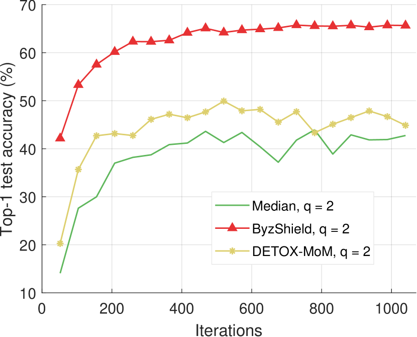
Figure 9: ALIE attack and median-based defenses (CIFAR-10), $K=15$.

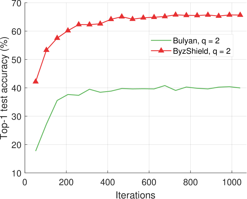
Figure 10: ALIE attack and Bulyan-based defenses (CIFAR-10), $K=15$

Table 4: Distortion fraction evaluation for Ramanujan-based assignment (Case 2) for $(m,s)=(5,5)$, i.e., $(K,f,l,r)=(25,25,5,5)$ and comparison.

$q$	$c_{\mathrm{max}}^{(q)}$	$\hat{\epsilon}^{ByzShield}$	$\hat{\epsilon}^{Baseline}$	$\hat{\epsilon}^{FRC}$	$\gamma$
$3$	1	0.04	0.12	0.2	2.43
$4$	1	0.04	0.16	0.2	3.9
$5$	2	0.08	0.2	0.2	5.56
$6$	4	0.16	0.24	0.4	7.35
$7$	5	0.2	0.28	0.4	9.25
$8$	7	0.28	0.32	0.4	11.23
$9$	9	0.36	0.36	0.6	13.28
$10$	12	0.48	0.4	0.6	15.38
$11$	14	0.56	0.44	0.6	17.54
$12$	17	0.68	0.48	0.8	19.73

Table 5: Distortion fraction evaluation for MOLS-based assignment for $(K,f,l,r)=(35,49,7,5)$ and comparison.

$q$	$c_{\mathrm{max}}^{(q)}$	$\hat{\epsilon}^{ByzShield}$	$\hat{\epsilon}^{Baseline}$	$\hat{\epsilon}^{FRC}$	$\gamma$
$3$	1	0.02	0.12	0.14	2.68
$4$	1	0.02	0.16	0.14	4.39
$5$	2	0.04	0.2	0.14	6.36
$6$	4	0.08	0.24	0.29	8.54
$7$	5	0.1	0.28	0.29	10.89
$8$	8	0.16	0.32	0.29	13.37
$9$	10	0.2	0.36	0.43	15.97
$10$	11	0.22	0.4	0.43	18.67
$11$	14	0.29	0.44	0.43	21.44
$12$	16	0.33	0.48	0.57	24.29
$13$	20	0.41	0.52	0.57	27.2

Table 6: Distortion fraction evaluation for MOLS-based assignment for $(K,f,l,r)=(21,49,7,3)$ and comparison.

$q$	$c_{\mathrm{max}}^{(q)}$	$\hat{\epsilon}^{ByzShield}$	$\hat{\epsilon}^{Baseline}$	$\hat{\epsilon}^{FRC}$	$\gamma$
$2$	1	0.02	0.1	0.14	2.23
$3$	3	0.06	0.14	0.14	4.67
$4$	5	0.1	0.19	0.29	7.72
$5$	8	0.16	0.24	0.29	11.29
$6$	12	0.24	0.29	0.43	15.27
$7$	16	0.33	0.33	0.43	19.6
$8$	21	0.43	0.38	0.57	24.22
$9$	25	0.51	0.43	0.57	29.08
$10$	29	0.59	0.52	0.71	34.15

Table 7: Parameters used for training.

Figure	Schemes	Learning rate schedule
4	$1,2$	$(0.00625,0.96,15)$
4	$3$	$(0.025,0.96,15)$
4	$4,5,6$	$(0.01,0.95,20)$
4	$1,2$	$(0.003125,0.96,15)$
4	$1$	$(0.00625,0.96,15)$
4	$2,5,6$	$(0.01,0.95,20)$
7	$1,2$	$(0.0001,0.99,20)$
7	$3,4$	$(0.025,0.96,15)$
7	$5,6$	$(0.001,0.5,50)$
7	$1,2,4$	$(0.05,0.96,15)$
7	$3$	$(0.1,0.95,50)$
7	$5,6$	$(0.025,0.96,15)$
7	$1,2$	$(0.025,0.96,15)$
7	$4$	$(0.05,0.96,15)$
8	$1,2,3$	$(0.05,0.96,15)$
8	$7,8$	$(0.025,0.96,15)$
11	$1$	$(0.003125,0.96,15)$
11	$2$	$(0.01,0.96,15)$
11	$3$	$(0.0125,0.96,15)$
11	$1$	$(0.0015625,0.96,15)$
11	$1$	$(0.003125,0.96,15)$
11	$3$	$(0.0125,0.96,15)$

References

- Abadi et al. (2016) Abadi, M., Barham, P., Chen, J., Chen, Z., Davis, A., Dean, J., Devin, M., Ghemawat, S., Irving, G., Isard, M., Kudlur, M., Levenberg, J., Monga, R., Moore, S., Murray, D. G., Steiner, B., Tucker, P., Vasudevan, V., Warden, P., Wicke, M., Yu, Y., and Zheng, X. TensorFlow: A system for large-scale machine learning. In 12th USENIX Symposium on Operating Systems Design and Implementation (OSDI 16), pp. 265–283, November 2016.
- Alon (1986) Alon, N. Eigenvalues and expanders. Combinatorica, 6(2):83––96, January 1986.
- Baruch et al. (2019) Baruch, G., Baruch, M., and Goldberg, Y. A little is enough: Circumventing defenses for distributed learning. In Advances in Neural Information Processing Systems 32, pp. 8635–8645, December 2019.
- Bernstein et al. (2019) Bernstein, J., Zhao, J., Azizzadenesheli, K., and Anandkumar, A. signSGD with majority vote is communication efficient and fault tolerant, 2019.
- Blanchard et al. (2017) Blanchard, P., El Mhamdi, E. M., Guerraoui, R., and Stainer, J. Machine learning with adversaries: Byzantine tolerant gradient descent. In Advances in Neural Information Processing Systems 30, pp. 119–129, December 2017.
- Boyer & Moore (1991) Boyer, R. S. and Moore, J. S. MJRTY—A Fast Majority Vote Algorithm. Springer Netherlands, Dordrecht, 1991.
- Burnwal et al. (2020) Burnwal, S. P., Sinha, K., and Vidyasagar, M. New and explicit constructions of unbalanced Ramanujan bipartite graphs, 2020.
- Chen et al. (2018) Chen, L., Wang, H., Charles, Z., and Papailiopoulos, D. DRACO: Byzantine-resilient distributed training via redundant gradients. In Proceedings of the 35th International Conference on Machine Learning, pp. 903–912, July 2018.
- Chen et al. (2015) Chen, T., Li, M., Li, Y., Lin, M., Wang, N., Wang, M., Xiao, T., Xu, B., Zhang, C., and Zhang, Z. MXNet: A flexible and efficient machine learning library for heterogeneous distributed systems, 2015.
- Chen et al. (2017) Chen, Y., Su, L., and Xu, J. Distributed statistical machine learning in adversarial settings: Byzantine gradient descent. Proc. ACM Meas. Anal. Comput. Syst., 1(2), December 2017.
- Chung (1997) Chung, F. R. K. Spectral Graph Theory. American Mathematical Society, Rhode Island, 1997.
- Damaskinos et al. (2019) Damaskinos, G., El Mhamdi, E. M., Guerraoui, R., Guirguis, A. H. A., and Rouault, S. L. A. Aggregathor: Byzantine machine learning via robust gradient aggregation. In Conference on Systems and Machine Learning (SysML) 2019, pp. 19, March 2019.
- Data et al. (2018) Data, D., Song, L., and Diggavi, S. Data encoding for Byzantine-resilient distributed gradient descent. In 2018 56th Annual Allerton Conference on Communication, Control, and Computing (Allerton), pp. 863–870, October 2018.
- Dean et al. (2012) Dean, J., Corrado, G., Monga, R., Chen, K., Devin, M., Mao, M., Ranzato, M. A., Senior, A., Tucker, P., Yang, K., Le, Q. V., and Ng, A. Y. Large scale distributed deep networks. In Advances in Neural Information Processing Systems 25, pp. 1223–1231, December 2012.
- El Mhamdi et al. (2018) El Mhamdi, E. M., Guerraoui, R., and Rouault, S. The hidden vulnerability of distributed learning in Byzantium. In Proceedings of the 35th International Conference on Machine Learning, pp. 3521–3530, July 2018.
- Fan (2001) Fan, J. L. Array Codes as LDPC Codes. Springer US, Boston, MA, 2001.
- Gunawi et al. (2018) Gunawi, H. S., Suminto, R. O., Sears, R., Golliher, C., Sundararaman, S., Lin, X., Emami, T., Sheng, W., Bidokhti, N., McCaffrey, C., Grider, G., Fields, P. M., Harms, K., Ross, R. B., Jacobson, A., Ricci, R., Webb, K., Alvaro, P., Runesha, H. B., Hao, M., and Li, H. Fail-slow at scale: Evidence of hardware performance faults in large production systems. In 16th USENIX Conference on File and Storage Technologies (FAST 18), pp. 1–14, February 2018.
- He et al. (2016) He, K., Zhang, X., Ren, S., and Sun, J. Deep residual learning for image recognition. In IEEE Conference on Computer Vision and Pattern Recognition (CVPR), pp. 770–778, June 2016.
- Høholdt & Janwa (2012) Høholdt, T. and Janwa, H. Eigenvalues and expansion of bipartite graphs. Des. Codes Cryptogr., 65(3):259–273, January 2012.
- Horn & Johnson (2012) Horn, R. A. and Johnson, C. R. Matrix Analysis. Cambridge University Press, New York, 2012.
- Kotla et al. (2007) Kotla, R., Alvisi, L., Dahlin, M., Clement, A., and Wong, E. Zyzzyva: Speculative Byzantine fault tolerance. SIGOPS Oper. Syst. Rev., 41(6):45––58, October 2007.
- Milenkovic & Laendner (2004) Milenkovic, O. and Laendner, S. Analysis of the cycle-structure of LDPC codes based on Latin squares. In 2004 IEEE International Conference on Communications (IEEE Cat. No.04CH37577), pp. 777–781, July 2004.
- Minsker (2015) Minsker, S. Geometric median and robust estimation in Banach spaces. Bernoulli, 21(4):2308–2335, November 2015.
- Paszke et al. (2019) Paszke, A., Gross, S., Massa, F., Lerer, A., Bradbury, J., Chanan, G., Killeen, T., Lin, Z., Gimelshein, N., Antiga, L., Desmaison, A., Kopf, A., Yang, E., DeVito, Z., Raison, M., Tejani, A., Chilamkurthy, S., Steiner, B., Fang, L., Bai, J., and Chintala, S. PyTorch: An imperative style, high-performance deep learning library. In Advances in Neural Information Processing Systems 32, pp. 8024–8035, December 2019.
- Rajput et al. (2019) Rajput, S., Wang, H., Charles, Z., and Papailiopoulos, D. DETOX: A redundancy-based framework for faster and more robust gradient aggregation. In Advances in Neural Information Processing Systems 32, pp. 10320–10330, December 2019.
- Raviv et al. (2018) Raviv, N., Tandon, R., Dimakis, A., and Tamo, I. Gradient coding from cyclic MDS codes and expander graphs. In Proceedings of the 35th International Conference on Machine Learning, pp. 4302–4310, July 2018.
- Seide & Agarwal (2016) Seide, F. and Agarwal, A. CNTK: Microsoft’s open-source deep-learning toolkit. In Proceedings of the 22nd ACM SIGKDD International Conference on Knowledge Discovery and Data Mining, pp. 2135, August 2016.
- Shen et al. (2016) Shen, S., Tople, S., and Saxena, P. Auror: Defending against poisoning attacks in collaborative deep learning systems. In Proceedings of the 32nd Annual Conference on Computer Security Applications, pp. 508––519, December 2016.
- Sipser & Spielman (1996) Sipser, M. and Spielman, D. A. Expander codes. IEEE Transactions on Information Theory, 42(6):1710–1722, November 1996.
- Tandon et al. (2017) Tandon, R., Lei, Q., Dimakis, A. G., and Karampatziakis, N. Gradient coding: Avoiding stragglers in distributed learning. In 34th International Conference on Machine Learning, pp. 3368–3376, August 2017.
- Van Lint & Wilson (2001) Van Lint, J. H. and Wilson, R. M. A Course in Combinatorics. Cambridge University Press, New York, 2001.
- Xie et al. (2018) Xie, C., Koyejo, O., and Gupta, I. Generalized Byzantine-tolerant SGD, 2018.
- Yin et al. (2018) Yin, D., Chen, Y., Kannan, R., and Bartlett, P. Byzantine-robust distributed learning: Towards optimal statistical rates. In Proceedings of the 35th International Conference on Machine Learning, pp. 5650–5659, July 2018.
- Yin et al. (2019) Yin, D., Chen, Y., Ramchandran, K., and Bartlett, P. L. Defending against saddle point attack in Byzantine-robust distributed learning. In Proceedings of the 36th International Conference on Machine Learning, pp. 7074–7084, June 2019.
- Yu et al. (2019) Yu, Q., Li, S., Raviv, N., Kalan, S. M. M., Soltanolkotabi, M., and Avestimehr, S. Lagrange coded computing: Optimal design for resiliency, security and privacy, 2019.
- Zhu & Chugg (2007) Zhu, M. and Chugg, K. M. Bounds on the expansion properties of Tanner graphs. IEEE Transactions on Information Theory, 53(12):4834–4841, December 2007.