A novel exact magnetic black hole solution in four-dimensional extended scalar-tensor-Gauss-Bonnet theory

Abstract

In this work the first exact asymptotically flat static and spherically symmetric black hole solution for $(3+1)$-dimensional ESTGB is presented, with a model of nonlinear electrodynamics -that reduces to Maxwell’s theory in the weak field limit and satisfies the weak energy condition- as a source. The solution has a nonzero magnetic charge, and scalar hair, which turns out to be dependent of the magnetic charge. It is characterized by the ADM mass $m$ and the magnetic charge $q$. Depending on the range of these parameters, the solution describes black holes with different structure. In the case $m\geq 0$ and $q\geq 0$, it shares many of the characteristics of the Schwarzschild solution. For $m>0$ and $q<0$, it is akin to the Reissner-Nordström metric. In the case $m=0$, it represents a purely magnetic black hole.

I Introduction

Many observational results and theoretical considerations have led to the idea that Einstein’s theory of General Relativity (GR) may not be valid in the high and/or low-curvature regimes. Among them we can mention the present stage of cosmic acceleration (see Yang2019 and references therein), the flatness of the rotation curves of galaxies (see for instance Capo2006 ), the union of gravity with the laws of quantum physics (see for instance Fradkin1985 ), and current limits on the tensor-to-scalar ratio Akrami2018 . Most of the extensions of GR involve additional degrees of freedom, such as those coming from a scalar field and/or curvature corrections to the Einstein-Hilbert Lagrangian, coupled to the scalar field. A particular and interesting extension, since it avoids the Ostrogradski instability, is given by the coupling of the scalar field with the Gauss-Bonnet invariant, which yields the so-called extended scalar-tensor-Gauss-Bonnet (ESTGB) (see scalariz_Doneva for details) . Such a theory follows at the level of the effective action of string theory, when viewed in the Einstein frame eff .

Various aspects of the ESTGB theory have been studied in detail lately. To name just a few applications in cosmology, it was shown in cosmic_acceleration that the theory can describe the present stage of cosmic acceleration, and can lead to an exit from a scaling matter-dominated epoch to a late-time accelerated expansion Tsujikawa2006 . The possible reconstruction of the coupling and potential functions for a given scale factor was considered in recon , and the consequences of ESTGB in an inflationary setting have been considered in Odintsov2020 .

Black hole solutions have been extensively discussed in ESTGB in $(3+1)$-dimensions, without matter fields. Given the complexity of the field equations, at present there are only numerical solutions available. In particular, and restricting to the static and spherically symmetric case, new black hole were shown to form by spontaneous scalarization -induced by the curvature of the geometry- of the Schwarzschild black holes in the extreme curvature regime in Doneva2018 ; scalariz_Silva (see Doneva2019 for a case of a massive scalar field, scalariz_Doneva for the charged case, kanti96 for the dilatonic case, and Doneva2020 for the multi-scalar case). There are also numerical solutions displaying “natural scalarization”, such as those presented in Kanti2018 ; Ultra_compact ; Antoniou18 ). Since all the solutions found in the literature are numerical, it would be of interest to find analytical solutions. We would like to present here the first solution of such a kind, using nonlinear electrodynamics (NLED) as a source.

Maxwell’s electrodynamics is a very well-established theory which has been subjected to innumerable tests. However, there are good theoretical reasons to consider modifications to it. For instance, with the aim of avoiding the divergent behavior associated to the electric field and the self-energy of a point charge, M. Born and L. Infeld NLED proposed a modified version of Maxwell’s theory that was a nonlinear function of the two electromagnetic invariants, namely $\mathcal{F}=2(\mathcal{B}^{2}-\mathcal{E}^{2})$ and $\mathcal{G}=\mathcal{E}\!\cdot\!\mathcal{B}$.

The explicit form of the Lagrangian $\mathcal{L}(\mathcal{F},\mathcal{G})$ may be determined according to different criteria , but there are two examples that are particularly relevant: that of the Born-Infeld theory mentioned above, and the Euler-Heisenberg theory Euler_Heisenberg , derived from one-loop quantum electrodynamics, that describes some nonlinear processes, like the light-by-light scattering. The latter is a quantum-mechanical process that is forbidden in classical electrodynamics. This reaction is accessible at the Large Hadron Collider thanks to the large electromagnetic field strengths generated by ultra-relativistic colliding lead ions (see for details lightbylight , where experimental evidence for light-by-light scattering has been reported).

It can also be added that the coupling of GR with NLED has led to a number of interesting solutions and phenomena. Among them we can mention black holes with everywhere-regular curvature invariants and electric field (see for instance BH_NLED ); traversables wormholes sustained with nonlinear electromagnetic fields WH_NLED ; non-gravitational wormholes Baldovin2000 , and a new entropy bound Falciano2019 .

In this article, the first exact black hole solution derived for $(3+1)-$dimensional extended scalar-tensor-Gauss-Bonnet theory (ESTGB) coupled to a particular form of nonlinear electrodynamics (NLED) is presented . The electromagnetic Lagrangian is such that it reduces to that of Maxwell in the weak field limit. The solution is analyzed in detail, and it is shown that, depending on the parameters that determine the spacetime metric, black holes with different features are allowed. The paper is organized as follows: in the next section we briefly outline the field equations derived from the ESTGB-NLED action. In Sect. IV the derived two-parametric family of solutions is presented, its black hole interpretation is analyzed, are treated the limiting cases of vanishing electromagnetic and scalar field, and vanishing of the ADM mass. Final conclusions are given in the last section. In this paper we use units where $G=c=1$.

II Extended Scalar-Tensor-Gauss-Bonnet gravity

The $(3+1)$-dimensional extended scalar-tensor-Gauss-Bonnet theory with additional matter fields, is defined by the following action,

$$S[g_{ab},\phi,\psi_{a}]=\int d^{4}x\sqrt{-g}\left\{\frac{1}{16\pi}\left(R-\frac{1}{2}\partial_{\mu}\phi\partial^{\mu}\phi+\bm{f}(\phi)R_{{}_{GB}}^{2}-2\mathscr{U}(\phi)\right)-\frac{1}{4\pi}\mathcal{L}_{\rm matter}(g_{ab},\psi_{a})\right\}.$$ (1)

The first term in this action defines the Einstein-Hilbert Lagrangian density. The Lagrangian density for the STGB contribution is defined by the addition of the kinetic term of the scalar field, the quadratic Gauss-Bonnet term $R_{{}_{GB}}^{2}$ non-minimally coupled to the scalar field, by the function $\bm{f}(\phi)$, and the scalar field potential $\mathscr{U}(\phi)$. The Lagrangian density $\mathcal{L}_{\rm matter}(g_{ab},\psi_{a})$ represents any matter fields present in the system. In this work, we will consider the ESTGB theory in the presence of non-linear electrodynamics (NLED), in which the Lagrangian is a function on the electromagnetic invariant $\mathcal{F}=F_{\alpha\beta}F^{\alpha\beta}/4$, with $F_{ab}=2\partial_{[a}A_{b]}$, and $A_{a}$ the electromagnetic potential. The ESTGB-NLED field equations arising from the variation of the action with respect to $g_{ab}$ are

$$G_{a}{}^{b}=8\pi(E_{a}{}^{b})\!_{{}_{{}_{G\!B}}}+8\pi(E_{a}{}^{b})\!_{{}_{{}_{N\!L\!E\!D}}},$$ (2)

where $G_{a}{}^{b}=R_{a}{}^{b}-\frac{R}{2}\delta_{a}{}^{b}$ denotes the components of the Einstein tensor, and the quantities $(E_{a}{}^{b})\!_{{}_{{}_{G\!B}}}$ and $(E_{a}{}^{b})\!_{{}_{{}_{N\!L\!E\!D}}}$ are defined by the following expressions:

$$8\pi(E_{\alpha}{}^{\beta})\!_{{}_{{}_{G\!B}}}=-\frac{1}{4}(\partial_{\mu}\phi\partial^{\mu}\phi)\delta_{\alpha}{}^{\beta}+\frac{1}{2}\partial_{\alpha}\phi\partial^{\beta}\phi-\frac{1}{2}(g_{\alpha\rho}\delta_{\lambda}{}^{\beta}+g_{\alpha\lambda}\delta_{\rho}{}^{\beta})\eta^{\mu\lambda\nu\sigma}\tilde{R}^{\rho\xi}{}_{\nu\sigma}\nabla_{\xi}\partial_{\mu}\bm{f}(\phi)-\mathscr{U}(\phi)\delta_{\alpha}{}^{\beta},$$ (3)

$$8\pi(E_{\alpha}{}^{\beta})\!_{{}_{{}_{N\!L\!E\!D}}}=2\left(\mathcal{L}_{\mathcal{F}}\hskip 0.56917ptF_{\alpha\mu}F^{\beta\mu}-\mathcal{L}\hskip 0.85355pt\delta_{\alpha}{}^{\beta}\right),$$ (4)

with $\tilde{R}^{\rho\gamma}{}_{\mu\nu}=\eta^{\rho\gamma\sigma\tau}R_{\sigma\tau\mu\nu}=\epsilon^{\rho\gamma\sigma\tau}R_{\sigma\tau\mu\nu}/\sqrt{-g}$, and $\mathcal{L}_{\mathcal{F}}\equiv\frac{d\mathcal{L}}{d\mathcal{F}}$ . Thus, $(E_{\alpha}{}^{\beta})\!_{{}_{{}_{G\!B}}}$ denotes the components of a tensor which we shall refer to as the Scalar-Gauss-Bonnet tensor, since it represents the contribution to the spacetime curvature due to the effects of the STGB term. The components of the NLED energy-momentum tensor are denoted by $(E_{\alpha}{}^{\beta})\!_{{}_{{}_{N\!L\!E\!D}}}$. The structure of the field equations (2) motives the definition of the effective energy-momentum tensor, $\mathscr{E}_{a}{}^{b}$, as $\mathscr{E}_{a}{}^{b}=(E_{a}{}^{b})\!_{{}_{{}_{G\!B}}}+(E_{a}{}^{b})\!_{{}_{{}_{N\!L\!E\!D}}}$. Thus, the ESTGB-NLED theory can be written in a GR-like form, $G_{a}{}^{b}=8\pi\mathscr{E}_{a}{}^{b}$.

By taking the divergence of Eq.(2), and taking into account that $\nabla_{\beta}(E_{\alpha}{}^{\beta})\!_{{}_{{}_{N\!L\!E\!D}}}=0$, and that the Bianchi identities guarantee that $\nabla_{\beta}G_{\alpha}{}^{\beta}=0$, it follows that $\nabla_{\beta}(E_{\alpha}{}^{\beta})\!_{{}_{{}_{G\!B}}}=0$. This in turn implies that

$$\nabla^{2}\phi+\dot{\bm{f}}(\phi)R_{{}_{GB}}^{2}+2\dot{\mathscr{U}}(\phi)=0,$$ (5)

where the overdot denotes the derivatives with respect to the scalar field, i.e., ($\dot{\bm{f}}=\frac{d\bm{f}}{d\phi}$, $\dot{\mathscr{U}}=\frac{d\mathscr{U}}{d\phi}$).

The equations of motion for the nonlinear electrodynamical theory are given by

$$\nabla_{\alpha}(\mathcal{L}_{\mathcal{F}}F^{\alpha\beta})=0,\;\;\;\;\;\;\;\;\;\;\nabla_{\alpha}(_{\ast}\!\bm{F})^{\alpha}=0,$$ (6)

where ${}_{\ast}\!\bm{F}$ denotes the Hodge star operation (or Hodge dual) with respect to the metric. Our aim is to find a exact solution of the set of Eqs. (2), (5), and (6), that describe an asymptotically flat, static and spherically symmetric black hole (AF-SSS-BH). Therefore, we will assume that the scalar field is static and spherically symmetric, $\phi=\phi(r)$, the electromagnetic invariant depends only on the radial coordinate, $\mathcal{F}=\mathcal{F}(r)$, and also that the metric takes the static and spherically symmetric form,

$$ds^{2}=-e^{A(r)}dt^{2}+e^{B(r)}dr^{2}+r^{2}(d\theta^{2}+\sin^{2}\theta d\varphi^{2}),$$ (7)

with $A=A(r)$ and $B=B(r)$ unknown functions of $r$.

Regarding the electromagnetic field tensor, since the spacetime is static and spherically symmetric, then the only non-vanishing terms are the electric component $F_{tr}=\mathcal{E}(r)$ and the magnetic component $F_{\theta\varphi}=\mathcal{B}(r,\theta)=h(r)\sin\theta$. In this work we restrict ourselves to a purely magnetic field, i.e., $\mathcal{E}(r)=0$ and $\mathcal{B}(r,\theta)\neq 0$. In this way, for a static and spherically symmetric spacetime with line element (7), the general solution of Eq. (6) is given by,

$$F_{\theta\varphi}=r^{4}\mathcal{Q}(r)\sin\theta.$$ (8)

Then, $\bm{F}=r^{4}\mathcal{Q}(r)d\theta\wedge d\varphi$, therefore $d\bm{F}=0=(r^{4}\mathcal{Q}(r))^{\prime}dr\wedge d\theta\wedge d\varphi$, (where the prime denotes the derivative with respect to the radial coordinate $r$) yields $\mathcal{Q}(r)=\sqrt{2}\hskip 1.70709ptq/r^{4}$, where $\sqrt{2}\hskip 1.70709ptq$ is an integration constant, which it plays the role of the magnetic charge. Hence, the components of the electromagnetic field tensor, and the invariant $\mathcal{F}$ are respectively given by;

$$F_{\alpha\beta}=F_{\theta\varphi}(\delta_{\alpha}^{\theta}\delta_{\beta}^{\varphi}-\delta_{\alpha}^{\varphi}\delta_{\beta}^{\theta}),\quad\quad\quad\quad\quad F_{\theta\varphi}=\mathcal{B}(\theta)=\sqrt{2}\hskip 1.70709ptq\sin\theta,\quad\quad\quad\quad\quad\mathcal{F}=\frac{q^{2}}{r^{4}}.$$ (9)

III Field equations

For the line element (7), the non-null components of the Einstein tensor are given by

$$G_{t}{}^{t}\!=\!\frac{e^{{}^{\!\!-B}}\left(\!-rB^{\prime}-e^{{}^{\!B}}+1\!\right)}{r^{2}}\!,\hskip 5.40608ptG_{r}{}^{r}\!=\!\frac{e^{{}^{\!\!-B}}\left(\!rA^{\prime}-e^{{}^{\!B}}+1\!\right)}{r^{2}}\!,\hskip 5.40608ptG_{\theta}{}^{\theta}\!=\!G_{\varphi}{}^{\varphi}\!=\!\frac{e^{{}^{\!\!-B}}\left(rA^{\prime 2}-rA^{\prime}B^{\prime}+2rA^{\prime\prime}+2A^{\prime}-2B^{\prime}\right)}{4r}\!.$$ (10)

The non-vanishing components of the SGB tensor with arbitrary coupling function $\bm{f}(\phi)$ and potential $\mathscr{U}$ are

$$8\pi(E_{t}{}^{t})\!_{{}_{{}_{G\!B}}}=-\frac{e^{-2B}}{4r^{2}}\left\{\left[r^{2}e^{B}+16(e^{B}-1)\ddot{\bm{f}}\right]\phi^{\prime 2}-8[(e^{B}-3)B^{\prime}\phi^{\prime}-2(e^{B}-1)\phi^{\prime\prime}]\dot{\bm{f}}\right\}-\mathscr{U},$$ (11)

$$8\pi(E_{r}{}^{r})\!_{{}_{{}_{G\!B}}}=\frac{e^{-B}\phi^{\prime}}{4}\left[\phi^{\prime}-\frac{8(e^{B}-3)e^{-B}A^{\prime}\dot{\bm{f}}}{r^{2}}\right]-\mathscr{U},$$ (12)

$$8\pi(E_{\theta}{}^{\theta})\!_{{}_{{}_{G\!B}}}=(E_{\varphi}{}^{\varphi})\!_{{}_{{}_{G\!B}}}=-\frac{e^{-2B}}{4r}\left\{(re^{B}-8A^{\prime}\ddot{\bm{f}})\phi^{\prime 2}-4\left[(A^{\prime 2}+2A^{\prime\prime})\phi^{\prime}+(2\phi^{\prime\prime}-3B^{\prime}\phi^{\prime})A^{\prime}\right]\dot{\bm{f}}\right\}-\mathscr{U}.$$ (13)

Finally, the energy-momentum tensor components for NLED, assuming the SSS spacetime with metric (7), the electromagnetic field tensor (9), and a Lagrangian density $\mathcal{L}(F)$, are given by

$$8\pi(E_{t}{}^{t})\!_{{}_{{}_{N\!L\!E\!D}}}=8\pi(E_{r}{}^{r})\!_{{}_{{}_{N\!L\!E\!D}}}=-2\mathcal{L},\quad\quad\quad 8\pi(E_{\theta}{}^{\theta})\!_{{}_{{}_{N\!L\!E\!D}}}=8\pi(E_{\varphi}{}^{\varphi})\!_{{}_{{}_{N\!L\!E\!D}}}=2(2\mathcal{F}\mathcal{L}_{\mathcal{F}}-\mathcal{L}).$$ (14)

Inserting the above given components in the field equations (2), we obtain:

$$\!G_{t}{}^{t}\!=\!8\pi\mathscr{E}_{t}{}^{t}\!\hskip 5.69046pt\Rightarrow\hskip 5.69046pt4e^{B}\!\!\left(rB^{\prime}\!+\!e^{B}\!-\!1\right)\!=\!\!\left[r^{2}e^{B}\!+\!16(e^{B}\!-\!1)\ddot{\bm{f}}\right]\!\!\phi^{\prime 2}\!-\!8\!\left[(e^{B}\!-\!3)B^{\prime}\phi^{\prime}\!-\!2(e^{B}\!-\!1)\phi^{\prime\prime}\right]\!\!\dot{\bm{f}}\!+\!4r^{2}e^{2B}(\mathscr{U}\!+\!2\mathcal{L}),$$ (15)

$$\!G_{r}{}^{r}\!=\!8\pi\mathscr{E}_{r}{}^{r}\!\hskip 3.27222pt\Rightarrow\hskip 3.27222pt4e^{B}\!\!\left(-rA^{\prime}\!+\!e^{B}\!-\!1\right)\!=\!-r^{2}e^{B}\phi^{\prime 2}\!+\!8(e^{B}\!-\!3)A^{\prime}\phi^{\prime}\dot{\bm{f}}\!+\!4r^{2}e^{2B}(\mathscr{U}\!+\!2\mathcal{L}),$$ (16)

$$\!G_{\theta}{}^{\theta}\!=\!8\pi\mathscr{E}_{\theta}{}^{\theta}\!\hskip 3.27222pt\Rightarrow\hskip 3.27222pte^{B}\!\!\left\{rA^{\prime 2}\!-\!2B^{\prime}\!+\!(2\!-\!rB^{\prime})A^{\prime}\!+\!2rA^{\prime\prime}\right\}\!=\!-re^{B}\phi^{\prime 2}\!+\!8A^{\prime}\ddot{\bm{f}}\phi^{\prime 2}$$

$$\hskip 196.32384pt\!+4\!\left[(A^{\prime 2}\!+\!2A^{\prime\prime})\phi^{\prime}\!+\!(2\phi^{\prime\prime}\!-\!3B^{\prime}\phi^{\prime})A^{\prime}\right]\!\!\dot{\bm{f}}\!-\!4re^{2B}(\mathscr{U}\!+\!2\mathcal{L}\!-\!4\mathcal{F}\mathcal{L}_{\mathcal{F}}).$$ (17)

The equation (5) for the scalar field $\phi$ can be written as

$$2r\phi^{\prime\prime}+(4+rA^{\prime}-rB^{\prime})\phi^{\prime}+\frac{4e^{-B}\dot{\bm{f}}}{r}\left[(e^{B}-3)A^{\prime}B^{\prime}-(e^{B}-1)(2A^{\prime\prime}+A^{\prime 2})\right]-4re^{B}\dot{\mathscr{U}}=0.$$ (18)

In the case with $\mathscr{U}(\phi)$=$\Lambda$=constant, and $\mathcal{L}(\mathcal{F})$=$0$, the system of equations (15), (16), (17) and (18), reduces to that for EGB gravity with a nonminimally coupled massless scalar field in the presence of a cosmological constant, see for instance Kanti2018 .

The problem of describing an AF-SSS magnetic black hole solution within the framework of ESTGB-NLED gravity, reduces to solving the field equations (15), (16), (17) and (18), with electromagnetic field (9), and SSS metric (7). It is useful to introduce the functions $\mathscr{M}$ and $\delta$ through

$$e^{A(r)}=\left(1-\frac{2\mathscr{M}\!(r)}{r}\right)e^{2\delta(r)},\quad\quad\quad\quad e^{B(r)}=\left(1-\frac{2\mathscr{M}\!(r)}{r}\right)^{-1},$$ (19)

where the mass function $\mathscr{M}\!(r)$ provides the ADM (Arnowitt-Deser-Misner) mass ($\mathscr{M}_{{}_{\!\!A\!D\!M}}$) in the asymptotic region, $\mathscr{M}_{{}_{\!\!A\!D\!M}}=\lim\limits_{r\rightarrow\infty}\mathscr{M}\!(r)\in\mathbb{R}^{+}$, and $\lim\limits_{r\rightarrow\infty}\delta(r)=0$, provided the spacetime is AF. The behavior of the scalar field $\phi$ in the limit $r\rightarrow\infty$ must be

$$\phi(r)=\phi_{0}+\phi_{1}/r+\phi_{2}/r^{2}+\mathcal{O}\!\left(r^{-3}\right),$$ (20)

with $\phi_{i}$ real parameters, and $\phi_{1}$ the scalar charge, see kanti96 ; Antoniou18 ; Kanti2018 ; Ultra_compact for details.

Regarding the NLED Lagrangian $\mathcal{L}(\mathcal{F})$, we shall impose, in agreement with Born and Infeld NLED , that it reduces to the Maxwell Lagrangian in the weak-field limit, i.e., $\mathcal{L}\rightarrow\kappa\hskip 1.42271pt\mathcal{F}$, $\mathcal{L}_{\mathcal{F}}\rightarrow\kappa$ (being $\kappa$ a constant), when $\mathcal{F}$ is very small. Furthermore, we shall require that the corresponding NLED energy-momentum tensor $(E_{a}{}^{b})\!_{{}_{{}_{N\!L\!E\!D}}}$ satisfies the weak energy condition (WEC), which states that for any timelike vector $\bm{k}=k^{\mu}\partial_{\mu}$, (i.e., $k_{\mu}k^{\mu}<0$), the tensor $(E_{a}{}^{b})\!_{{}_{{}_{N\!L\!E\!D}}}$ obeys the inequality $(E_{\mu\nu})\!_{{}_{{}_{N\!L\!E\!D}}}k^{\mu}k^{\nu}\geq 0$, which means that the local energy density $\rho_{\!{}_{{}_{loc}}}=(E_{\mu\nu})\!_{{}_{{}_{N\!L\!E\!D}}}k^{\mu}k^{\nu}$ as measured by any observer with timelike vector $\bm{k}$ is a non-negative quantity. Following WEC , for a diagonal energy-momentum tensor $(E_{\alpha\beta})=diag\left(E_{tt},E_{rr},E_{\theta\theta},E_{\varphi\varphi}\right)$, which can conveniently be written as

$$E_{\alpha}{}^{\beta}=-\rho\hskip 1.42271pt\delta_{\alpha}{}^{t}\delta_{t}{}^{\beta}+P_{r}\hskip 1.42271pt\delta_{\alpha}{}^{r}\delta_{r}{}^{\beta}+P_{\theta}\hskip 1.42271pt\delta_{\alpha}{}^{\theta}\delta_{\theta}{}^{\beta}+P_{\varphi}\hskip 1.42271pt\delta_{\alpha}{}^{\varphi}\delta_{\varphi}{}^{\beta},$$ (21)

WEC leads to

$$\rho=-E_{t}{}^{t}\geq 0,\quad\rho+P_{a}\geq 0,\quad a=\{r,\theta,\varphi\}.$$ (22)

IV An exact two-parametric family of solutions in ESTGB theory

Let us present now the specific choice of the relevant functions that leads to an exact static and spherically symmetric solution. $\bm{f}(\phi)$, $\mathscr{U}(\phi)$, and $\mathcal{L}$ are respectively given by

$$\bm{f}\! = \!-\frac{\ell^{2}\sigma}{32}\!\!\left\{\sqrt{2\sigma}\tan^{\!{}^{\!-1}}\!\!\!\left(\frac{\sqrt{2}}{\sqrt{\sigma}\hskip 1.70709pt\phi}\right)+\frac{1}{2\phi}\ln\!\!\left[\!\left(\!\!\frac{2\beta}{\sigma\phi^{2}}\!+\!\beta\!\!\right)^{\!\!\!2}\right]-\frac{2}{\phi}\right\}\!\!,$$ (23)

$$\mathscr{U}\!\! = \!\frac{2^{\!{}^{\frac{9}{2}}}}{105\ell^{2}\sigma^{\frac{7}{2}}}\!\left[\frac{\pi}{2}-\!\tan^{\!{}^{\!-1}}\!\!\!\left(\!\!\frac{\sqrt{2}}{\sqrt{\sigma}\hskip 1.70709pt\phi}\!\!\right)\right]\!+\!\frac{\phi^{5}}{4\ell^{2}}\!\!\left(\!\frac{3}{10\sigma}\!+\!\frac{5\phi^{2}}{7}\!+\!\frac{7\sigma\phi^{4}}{24}\!\right)\!\!\ln\!\!\left[\!\!\left(\!\!\frac{2\beta}{\sigma\phi^{2}}\!+\!\beta\!\!\right)^{\!\!\!2}\right]\!-\!\frac{\phi}{3\ell^{2}}\!\!\left(\!\frac{16}{35\sigma^{3}}\!-\!\frac{8\phi^{2}}{105\sigma^{2}}\!+\!\frac{31\phi^{4}}{70\sigma}\!+\!\frac{11\phi^{6}}{28}\!\right)\!\!,$$ (24)

$$\mathcal{L}\! = \!\frac{\mathcal{F}}{8}\!+\!\frac{8\mathcal{F}^{\frac{1}{4}}}{105\sigma_{\!\ast}^{3}s^{\frac{3}{2}}}\!-\!\frac{4\mathcal{F}^{\frac{3}{4}}}{315\sigma_{\!\ast}^{2}s^{\frac{1}{2}}}\!-\!\left(\!\frac{37}{210\sigma_{\!\ast}}\!+\!1\!\right)\!s^{\frac{1}{2}}\mathcal{F}^{\frac{5}{4}}\!-\!\frac{5s^{\frac{3}{2}}\mathcal{F}^{\frac{7}{4}}}{84}\!+\!\frac{2^{\!{}^{\frac{7}{2}}}}{105\sigma_{\!\ast}^{\frac{7}{2}}s^{2}}\!\left[\!\tan^{\!{}^{\!-1}}\!\!\!\left(\!\!\frac{\sqrt{2}}{\sqrt{s\sigma_{\!\ast}}\hskip 1.70709pt\mathcal{F}^{\frac{1}{4}}}\!\!\right)-\frac{\pi}{2}\right]$$ (25)

$$\hskip 153.6447pt-\frac{1}{2}\!\!\left(\!\frac{\mathcal{F}}{8}\!-\!\frac{3s^{\frac{1}{2}}\mathcal{F}^{\frac{5}{4}}}{10\sigma_{\!\ast}}\!+\!\frac{3\sigma_{\!\ast}s\mathcal{F}^{\frac{6}{4}}}{16}\!-\!\frac{4s^{\frac{3}{2}}\mathcal{F}^{\frac{7}{4}}}{7}\!-\!\frac{5\sigma_{\!\ast}s^{\frac{5}{2}}\mathcal{F}^{\frac{9}{4}}}{24}\!\right)\!\ln\!\!\left[\!\left(\!\frac{2\beta_{\ast}}{\sigma_{\!\ast}s\mathcal{F}^{\frac{1}{2}}}\!+\!\beta_{\ast}\!\right)^{\!\!2}\right]\!.$$

The constants $\ell$, $\sigma$, and $\beta$ belong to the ESTGB sector, while $s$, $\sigma_{\!\ast}$ and $\beta_{\ast}$, are in the NLED sector.

In order that the NLED Lagrangian shown in Eq.(25) reduces in the weak-field to Maxwell’s electrodynamics, we will assume that such Lagrangian is valid for $\mathcal{F}>\mathcal{F}_{{}_{0}}=\frac{4\beta^{2}_{\ast}}{s^{2}\sigma^{2}_{\!\ast}}$. Notice that $\mathcal{F}_{{}_{0}}$ can in principle be made as small as needed, by choosing the appropriate value of the constants in its definition. This minimum value guarantees the correct weak-field limit, as follows from the expansion of Eq.(25) for small $\mathcal{F}$:

$$\mathcal{L}\!=\!\frac{1}{8}\!\left[\!1\!-\!\frac{1}{2}\!\ln\!\!\left(\!\frac{4\beta_{\ast}^{2}}{\sigma_{\!\ast}^{2}s^{2}\mathcal{F}}\!\right)\!\right]\!\!\mathcal{F}\!-\!s^{{}^{\frac{1}{2}}}\!\!\!\left[1\!+\!\frac{37}{210\sigma_{\!\ast}}\!+\!\frac{2}{525\sigma_{\!\ast}}\!-\!\frac{3}{20\sigma_{\!\ast}}\ln\!\!\left(\!\frac{4\beta_{\ast}^{2}}{\sigma_{\!\ast}^{2}s^{2}\mathcal{F}}\!\right)\!\right]\!\!\mathcal{F}^{\frac{5}{4}}\!-\!\frac{\sigma_{\!\ast}s}{16}\!\left[\!1\!+\frac{3}{2}\ln\!\!\left(\!\frac{4\beta_{\ast}^{2}}{\sigma_{\!\ast}^{2}s^{2}\mathcal{F}}\!\right)\right]\!\!\mathcal{F}^{\frac{3}{2}}\!$$

$$\hskip 256.0748pt+\frac{s^{{}^{\frac{3}{2}}}}{7}\!\!\left[\!\frac{9}{14}\!+\!2\ln\!\!\left(\!\frac{4\beta_{\ast}^{2}}{\sigma_{\!\ast}^{2}s^{2}\mathcal{F}}\!\right)\!\right]\!\!\mathcal{F}^{\frac{7}{4}}\!-\!\frac{5s^{2}\sigma^{2}_{\!\ast}}{64}\!\mathcal{F}^{2}\!+\!\mathcal{O}\!\left(\mathcal{F}^{\frac{9}{4}}\right).$$ (26)

In the weak-field limit, $\mathcal{F}\rightarrow\mathcal{F}_{0}$, and $\ln\!\!\left(\!\frac{4\beta_{\ast}^{2}}{\sigma_{\!\ast}^{2}s^{2}\mathcal{F}}\!\right)\rightarrow 0$. Thus, in this limit Eq. (IV) becomes

$$\mathcal{L}\!=\!\frac{\mathcal{F}}{8}-s^{{}^{\frac{1}{2}}}\!\!\!\left(1\!+\!\frac{37}{210\sigma_{\!\ast}}\!+\!\frac{2}{525\sigma_{\!\ast}}\!\right)\!\mathcal{F}^{{}^{\frac{5}{4}}}-\frac{\sigma_{\!\ast}s\mathcal{F}^{{}^{\frac{3}{2}}}}{16}+\mathcal{O}(\mathcal{F}^{{}^{\frac{7}{4}}}).$$ (27)

Hence, under the assumption of the minimum value for $\mathcal{F}_{0}$, the NLED model (25) reduces in the weak-field limit to that of Maxwell’s electrodynamics: $\mathcal{L}\!\rightarrow\!\frac{1}{8}\mathcal{F}$, $\mathcal{L}_{\mathcal{F}}\!\rightarrow\!\frac{1}{8}$.

Let us move now to the new exact solution for the model defined by the equations given above. The ESTGB-NLED model we have presented admits a magnetic ESTGB-NLED exact solution for the case in which its parameters satisfy the relations

$$\sigma=\sigma_{\!\ast}=\frac{q}{m},\quad\quad\quad\ell=s=q,\quad\quad\quad\beta=\beta_{\ast}.$$ (28)

For such a solution, the line element is given by

$$ds^{2}=-\left(1-\frac{2m}{r}-\frac{q^{3}}{r^{3}}\right)dt^{2}+\left(1-\frac{2m}{r}-\frac{q^{3}}{r^{3}}\right)^{\!-1}dr^{2}+r^{2}(d\theta^{2}+\sin^{2}\theta d\varphi^{2}),$$ (29)

and the electromagnetic invariant is determined by Eq.(9). Finally, the scalar field is simply

$$\phi(r)=\frac{q}{r}.$$ (30)

It follows that the new black hole solution presented here has scalar hair, which is of the secondary kind, since it is not accompanied by any new quantity that characterizes the black hole. This is due to the relation between the magnetic and the scalar charge.

Comparing the metric given in Eq. (29) with Eq. (19), it follows that $\mathscr{M}\!(r)=m+\frac{q^{3}}{2r^{2}}$ and $\delta(r)=0$. Thus, the corresponding ADM mass will be $\mathscr{M}_{{}_{\!\!A\!D\!M}}=\lim\limits_{r\rightarrow\infty}\mathscr{M}\!(r)=m$. From Eqs.(20) and (30) it follows that the parameter $q$ corresponds to the scalar charge.

Evaluating the curvature invariants for this metric, we get

$$R=\frac{2q^{3}}{r^{5}},\quad R_{\alpha\beta}R^{\alpha\beta}=\frac{26q^{6}}{r^{10}},\quad R_{\alpha\beta\sigma\nu}R^{\alpha\beta\sigma\nu}=\frac{4(3m^{2}r^{4}+20mq^{3}r^{2}+46q^{6})}{r^{10}}.$$ (31)

Hence, analogously to the vacuum (or electrovacuum) AF-SSS black hole solutions in General Relativity, the origin $r=0$ is a physical singularity, and the solution here presented is regular everywhere else. We shall show below that the NLED satisfies the weak energy condition (WEC), which is defined as follows. From Eqs. (14) and (21), we obtain

$$\rho^{{}^{\!(\!N\!L\!E\!D\!)}}=\frac{\mathcal{L}}{4\pi},\quad\quad\quad\quad P_{r}^{{}^{\!(\!N\!L\!E\!D\!)}}=-\frac{\mathcal{L}}{4\pi},\quad\quad\quad\quad P_{\theta}^{{}^{\!(\!N\!L\!E\!D\!)}}=P_{\varphi}^{{}^{\!(\!N\!L\!E\!D\!)}}=\frac{2\mathcal{F}\mathcal{L}_{\mathcal{F}}-\mathcal{L}}{4\pi}.$$ (32)

Hence, according to (22), the NLED energy-momentum tensor (14) satisfies the WEC if

$$\rho^{{}^{\!(\!N\!L\!E\!D\!)}}=\frac{\mathcal{L}}{4\pi}\geq 0,\quad\rho^{{}^{\!(\!N\!L\!E\!D\!)}}+P^{{}^{\!(\!N\!L\!E\!D\!)}}_{r}=0,\quad\rho^{{}^{\!(\!N\!L\!E\!D\!)}}+P^{{}^{\!(\!N\!L\!E\!D\!)}}_{a}=\frac{\mathcal{F}\mathcal{L}_{\mathcal{F}}}{2\pi}\geq 0,\quad a=\{\theta,\varphi\}.$$ (33)

Since the invariant $\mathcal{F}$ is positive definite, see Eq.(9), then the WEC is holds if $\mathcal{L}\geq 0,$ $\mathcal{L}_{\mathcal{F}}\geq 0.$

It will also be required that the effective energy-momentum tensor satisfies the WEC. The components of this tensor in the case of the solution presented here are given by

$$\left(8\pi\mathscr{E}_{\nu}{}^{\mu}\right)={\rm diag}\!\left(\frac{2q^{3}}{r^{5}},\frac{2q^{3}}{r^{5}},-\frac{3q^{3}}{r^{5}},-\frac{3q^{3}}{r^{5}}\right).$$ (34)

Then, the comparison with Eq. (21) yields

$$\rho^{{}^{\!(\!e\!f\!f\!)}}=-\frac{2q^{3}}{8\pi r^{5}},\;\;\;\;\;\;\;P_{r}^{{}^{\!(\!e\!f\!f\!)}}=\frac{2q^{3}}{8\pi r^{5}},\;\;\;\;\;\;\;P_{\theta}^{{}^{\!(\!e\!f\!f\!)}}=P_{\varphi}^{{}^{\!(\!e\!f\!f\!)}}=-\frac{3q^{3}}{8\pi r^{5}}.$$

It follows that

$$\rho^{{}^{\!(\!e\!f\!f\!)}}+P_{r}^{{}^{\!(\!e\!f\!f\!)}}=0,\;\;\;\;\;\;\;{\rm and}\;\;\;\;\;\;\;\rho^{{}^{\!(\!e\!f\!f\!)}}+P_{\theta}^{{}^{\!(\!e\!f\!f\!)}}=\rho^{{}^{\!(\!e\!f\!f\!)}}+P_{\varphi}^{{}^{\!(\!e\!f\!f\!)}}=-\frac{5q^{3}}{8\pi r^{5}}.$$

Therefore, we conclude that if $q\leq 0$, the effective energy momentum tensor satisfies the WEC. This is in contrast with the ESTGB Maxwell, and ESTGB power-Maxwell, traversable wormhole solutions presented in Exact_wH_ED ; Exact_wH_NLED , for which the corresponding effective energy-momentum tensors violate the WEC in some regions of the spacetime.

Let us present next the properties of the solution and of the model according to the different possible choices of parameters in them.

IV.1 Horizons and black hole interpretations

We begin by showing that the metric given in Eq. (29) admits several AF-SSS-BH interpretations, depending on the range of the values taken by its parameters. The horizons are determined by the roots of the function $g_{tt}(r)=-(r^{3}-2mr^{2}-q^{3})/r^{3}$. In the general case, $g_{tt}$ can have three different roots which will be denoted by $x_{{}_{0}}$, $x_{{}_{1}}$, $x_{{}_{2}}$. However, a given root $r=x_{i}$ will correspond to the radius of the of a horizon only if $x_{i}\in\mathbb{R}^{+}$. The root $x_{{}_{0}}$ is given by

$$x_{{}_{0}}=\frac{2m}{3}+\frac{(108q^{3}+64m^{3}+12\sqrt{96m^{3}q^{3}+81q^{6}})^{\frac{1}{3}}}{6}+\frac{8m^{2}}{3(108q^{3}+64m^{3}+12\sqrt{96m^{3}q^{3}+81q^{6}})^{\frac{1}{3}}}.$$ (35)

$x_{0}$ can be used to write the metric component $g_{tt}$ as $g_{tt}=-(r-x_{{}_{0}})\!\!\left[r^{2}+(x_{{}_{0}}-2m)r+(x_{{}_{0}}^{2}-2mx_{{}_{0}})\right]/r^{3}$, and $x_{{}_{1}}$ and $x_{{}_{2}}$ are now the roots of the polynomial

$$\mathscr{P}(r)=r^{2}+(x_{{}_{0}}-2m)r+(x_{{}_{0}}-2m)x_{{}_{0}},$$ (36)

which are given by

$$x_{{}_{1}}=\frac{2m-x_{{}_{0}}+\sqrt{-3x_{{}_{0}}^{2}+4mx_{{}_{0}}+4m^{2}}}{2},\quad\quad\quad\quad\quad x_{{}_{2}}=\frac{2m-x_{{}_{0}}-\sqrt{-3x_{{}_{0}}^{2}+4mx_{{}_{0}}+4m^{2}}}{2}.$$ (37)

Several cases must be considered, according to the sign of the parameters involved:

IV.1.1 Case $\{m>0$, $q>0\}$

For this setting of parameters, it follows from Eq. (35) that $x_{0}$ is real. Hence, it corresponds to the radius of a horizon. Also, the following inequality is valid:

$$x_{{}_{0}}=\frac{2m}{3}+\frac{(108q^{3}+64m^{3}+12\sqrt{96m^{3}q^{3}+81q^{6}})^{\frac{1}{3}}}{6}+\frac{8m^{2}}{3(108q^{3}+64m^{3}+12\sqrt{96m^{3}q^{3}+81q^{6}})^{\frac{1}{3}}}\quad\geq\quad 2m$$ (38)

Given that $x_{{}_{0}}\geq 2m>0$ the roots of the polynomial $\mathscr{P}(r)$, given by Eq.(37) do not correspond to positive real numbers. Thus for this case the metric in Eq. (29) admits a AF-SSS-BH interpretation, with structure similar to the Schwarzschild metric, i.e., positive ADM mass, only one event horizon at the surface $r=x_{{}_{0}}$, and satisfying $g_{tt}(r)\rightarrow\infty$ as $r\rightarrow 0$. The plot of $-g_{tt}(r)$ in terms of the dimensionless coordinate $r/q$ is displayed in Fig. 1 for different values of $q/m$.

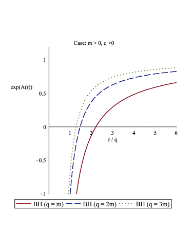
Figure 1: Behavior of $-g_{tt}$ for $m>0$ and $q>0$, with different values of $q/m$. In all cases, there is a single horizon.

IV.1.2 Case $\{m>0$, $q<0\}$

This case encompasses three sub-cases characterized by whether $96m^{3}q^{3}+81q^{6}$ is negative, null, or positive. For the sub-case $96m^{3}q^{3}+81q^{6}<0$, we can define

$$z_{{}_{0}}=108q^{3}+64m^{3}+12i\sqrt{-96m^{3}q^{3}-81q^{6}}=\rho_{{}_{0}}e^{i\theta_{{}_{0}}}\in\mathbb{C},\hskip 17.07182pt\textup{with}\hskip 11.38092pt\rho_{{}_{0}}=64m^{3},$$

$$\theta_{{}_{0}}\!=\!\tan^{{}^{-1}}\!\!\left(\frac{3\sqrt{-96q^{3}m^{3}-81q^{6}}}{|27q^{3}+16m^{3}|}\right)\hskip 8.5359pt\textup{if}\hskip 8.5359pt\mathcal{R}e(z_{{}_{0}})>0,\hskip 8.5359pt\theta_{{}_{0}}\!=\!\pi\!-\!\tan^{{}^{-1}}\!\!\left(\frac{3\sqrt{-96q^{3}m^{3}-81q^{6}}}{|27q^{3}+16m^{3}|}\right)\hskip 8.5359pt\textup{if}\hskip 8.5359pt\mathcal{R}e(z_{{}_{0}})<0.$$ (39)

Hence, $0<\theta_{{}_{0}}<\pi$, and $x_{{}_{0}}$ can be written as

$$x_{{}_{0}}=\frac{2m}{3}+\frac{1}{6}\rho^{\frac{1}{3}}_{{}_{0}}e^{\frac{1}{3}i\theta_{{}_{0}}}+\frac{8m^{2}}{3}\rho^{-\frac{1}{3}}_{{}_{0}}e^{-\frac{1}{3}i\theta_{{}_{0}}}=\frac{2m}{3}\!\!\left[1+2\cos\left(\frac{\theta_{{}_{0}}}{3}\right)\right].$$ (40)

leading to $\frac{4m}{3}<x_{{}_{0}}<2m$. Due to this restriction on $x_{0}$, the polynomial $\mathscr{P}(r)$ has two different real zeros, $x_{{}_{1}}$ and $x_{{}_{2}}$, given respectively by,

$$x_{{}_{1}}=\frac{2m-x_{{}_{0}}+\sqrt{-3x_{{}_{0}}^{2}+4mx_{{}_{0}}+4m^{2}}}{2}>0,\quad\quad\quad x_{{}_{2}}=\frac{2m-x_{{}_{0}}-\sqrt{-3x_{{}_{0}}^{2}+4mx_{{}_{0}}+4m^{2}}}{2}<0$$ (41)

with $0<x_{{}_{1}}<\frac{4m}{3}$. It follows that for this sub-case, in general way, the solution supports two horizons located at $r_{h}=x_{{}_{0}}$ (outer event horizon) and $r_{{}_{1}}=x_{{}_{1}}$ (inner horizon). Hence, this sub-case leads a non-extreme BH. On another hand, the sub-case $96m^{3}q^{3}+81q^{6}=0$ (which is equivalent to $\theta_{{}_{0}}=3\pi$), leads to $x_{{}_{0}}=-\frac{2}{3}m$, $r_{{}_{1}}=r_{{}_{2}}=x_{{}_{1}}=x_{{}_{2}}=\frac{4m}{3}$, which corresponds to an extreme black hole with event horizon given by $r_{h}=\frac{4m}{3}$. Finally, the sub-case $96m^{3}q^{3}+81q^{6}>0$ yields $x_{{}_{0}}$, $x_{{}_{1}}$, $x_{{}_{2}}$ $\not\in\mathbb{R}^{+}$, and then only for pairs $(m,q)$ that satisfy this condition the solution does not present an event horizon, leading to a naked singularity at $r=0$. Summarizing, when $\{m>0$, $q<0\}$, our solution has characteristics similar to those of the Reissner-Nordström metric. Fig. 2 shows the plot of $-g_{tt}(r)$ for a fixed values of $m/q$, corresponding to solutions a non-extreme BH, an extreme BH, and a naked singularity.

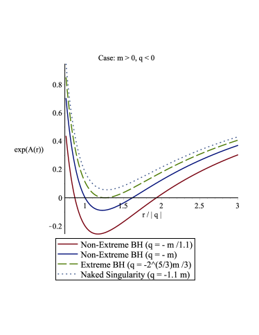
Figure 2: Behavior of $-g_{tt}$ for $m>0$ and $q<0$, with different values of $m/q$.

IV.1.3 Case $\{m<0$, $q>0\}$

Within this case, we consider the sub-case $96m^{3}q^{3}+81q^{6}\geq 0$. For this setting of parameters, the quantity $x_{{}_{0}}$ given by Eq.(35) is such that $x_{{}_{0}}\geq\frac{2|m|}{3}$. This implies that the roots of the polynomial $\mathscr{P}(r)=r^{2}+(x_{{}_{0}}-2m)r+(x_{{}_{0}}^{2}-2mx_{{}_{0}})$, are not positive real numbers. Whereas, if $96m^{3}q^{3}+81q^{6}\leq 0$, we can define

$$z_{{}_{0}}\!=\!108q^{3}+64m^{3}+12i\sqrt{-96q^{3}m^{3}-81q^{6}}\!=\!\rho_{{}_{0}}e^{i\theta_{{}_{0}}},\hskip 17.07182pt\textup{with}\hskip 11.38092pt\rho_{{}_{0}}\!=\!-64m^{3},$$ (42)

$$\theta_{{}_{0}}\!=\!\tan^{\!{}^{-1}}\!\!\left(\frac{3\sqrt{-96q^{3}m^{3}-81q^{6}}}{|27q^{3}+16m^{3}|}\right)\hskip 8.5359pt\textup{if}\hskip 8.5359pt\mathcal{R}e(z_{{}_{0}})>0,\hskip 8.5359pt\theta_{{}_{0}}\!=\!\pi\!-\!\tan^{\!{}^{-1}}\!\!\left(\frac{3\sqrt{-96q^{3}m^{3}-81q^{6}}}{|27q^{3}+16m^{3}|}\right)\hskip 8.5359pt\textup{if}\hskip 8.5359pt\mathcal{R}e(z_{{}_{0}})<0,$$ (43)

leading to $0<\theta_{{}_{0}}<\pi$. Hence, for this sub-case $x_{{}_{0}}$ is given by

$$x_{{}_{0}}=\frac{2m}{3}+\frac{1}{6}\rho^{\frac{1}{3}}_{{}_{0}}e^{\frac{1}{3}i\theta_{{}_{0}}}+\frac{8m^{2}}{3}\rho^{-\frac{1}{3}}_{{}_{0}}e^{-\frac{1}{3}i\theta_{{}_{0}}}=-\frac{2m}{3}\left(2\cos\left(\frac{\theta}{3}\right)-1\right),$$ (44)

which leads to $x_{{}_{0}}<\frac{2|m|}{3}$. Thus, since $x_{{}_{0}}>0$ and $m<0$, the roots of the polynomial $\mathscr{P}(r)$ do not correspond to positive real numbers.

Therefore, for the case $\{m<0$, $q>0\}$, the solution (29) can be interpreted as an AF-SSS-BH with negative ADM mass and only one horizon at $r=x_{{}_{0}}$. Plots of $-g_{tt}(r)$ for this case are presented in Fig. 3, for different values of $q/m$.

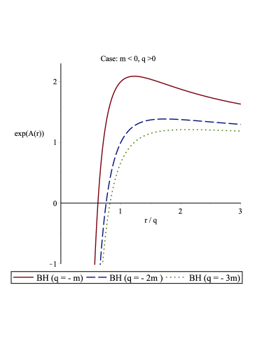
Figure 3: Behavior of $-g_{tt}$ for $m<0$ and $q>0$, with different values of $q/m$.

IV.1.4 Case $\{m<0$, $q<0\}$

For this case, all the roots of $g_{tt}(r)$ do not belong to $\mathbb{R}^{+}$. Then for this set of parameters the metric (29) represents a naked singularity .

IV.1.5 Restrictions imposed by the weak energy condition

Let us see now the restrictions that follow from taking into account that both the energy-momentum tensor associated to the NLED Lagrangian and the effective energy-momentum tensor have to fulfill the conditions dictated by the WEC. First, notice that following the discussion after Eq. (34), only solutions with $q<0$ are acceptable. Thus, from now on we shall restrict the analysis to the case ${m>0,q<0}$, since the rest of the cases lead to an effective energy-momentum tensors which does not satisfy the WEC. Consequently, the notation $Q=-q$ will be used from now on, with $Q>0$.

Regarding the WEC and the NLED energy-momentum tensor, we show next that the corresponding local NLED energy density is positive definite outside the black hole event horizon. In order to describe the behavior of $\mathcal{L}$ and $\mathcal{L}_{\mathcal{F}}$, we shall introduce the variable $\tilde{\mathcal{F}}$ defined by the rescaling, $\tilde{\mathcal{F}}=q^{2}\mathcal{F}$. Using Eq. (9) and $\tilde{\mathcal{F}}$ we can rewrite $\mathcal{L}$ given in Eq. (57) as a function of $\tilde{\mathcal{F}}$. The result is

$$Q^{2}\mathcal{L} = \frac{\tilde{\mathcal{F}}}{8}\!+\!\frac{8m^{3}}{105Q^{3}}\tilde{\mathcal{F}}^{\frac{1}{4}}\!+\!\frac{4m^{2}}{315Q^{2}}\tilde{\mathcal{F}}^{\frac{3}{4}}\!-\!\left(\!\frac{37m}{210Q}\!-\!1\!\right)\!\tilde{\mathcal{F}}^{\frac{5}{4}}\!+\!\frac{5}{84}\!\tilde{\mathcal{F}}^{\frac{7}{4}}\!-\!\frac{2^{\!{}^{\frac{3}{2}}}m^{\!{}^{\frac{7}{2}}}}{105Q^{\frac{7}{2}}}\!\ln\!\!\!\left[\!\!\left(\!\!\frac{\frac{\tilde{\mathcal{F}}^{{}^{\frac{1}{4}}}}{2^{{}^{\!\frac{1}{2}}}}\!+\!\frac{m^{{}^{\!\frac{1}{2}}}}{Q^{{}^{\!\frac{1}{2}}}}}{\frac{\tilde{\mathcal{F}}^{{}^{\frac{1}{4}}}}{2^{{}^{\!\frac{1}{2}}}}\!-\!\frac{m^{{}^{\!\frac{1}{2}}}}{Q^{{}^{\!\frac{1}{2}}}}}\!\!\right)^{\!\!\!2}\right]$$ (45)

$$\hskip 147.95424pt-\frac{1}{2}\!\left(\!\frac{\tilde{\mathcal{F}}}{8}\!-\!\frac{3m}{10Q}\tilde{\mathcal{F}}^{{}^{\frac{5}{4}}}\!-\!\frac{3Q}{16m}\tilde{\mathcal{F}}^{{}^{\frac{3}{2}}}\!+\!\frac{4}{7}\tilde{\mathcal{F}}^{{}^{\frac{7}{4}}}\!-\!\frac{5Q}{24m}\tilde{\mathcal{F}}^{{}^{\frac{9}{4}}}\!\right)\!\ln\!\!\left[\!\!\left(\!\frac{2m\beta}{Q\tilde{\mathcal{F}}^{{}^{\frac{1}{2}}}}\!-\!\beta\!\right)^{\!\!2}\right]\!\!,$$

The values of $r$ outside the black hole, given by $r\in(r_{h},\infty)$, with $r_{h}$ the outer event horizon, given by $r_{h}=x_{{}_{0}}$, see Eq. (40), or the single event horizon in the extremal case, give by $r_{h}=\frac{4m}{3}$, delimitate the domain of $q^{2}{\cal L}$, which is given by $\tilde{D}=\left[\tilde{\mathcal{F}}_{{}_{0}},\tilde{\mathcal{F}}_{{}_{h}}\right]$, where $\tilde{\mathcal{F}}_{{}_{0}}=q^{2}\mathcal{F}_{{}_{0}}=\frac{4\beta^{2}m^{2}}{q^{2}}$ is the minimum value of the rescaled variable, and $\tilde{\mathcal{F}}_{{}_{h}}=q^{2}\mathcal{F}_{{}_{h}}=\frac{q^{4}}{r^{4}_{{}_{h}}}$ its value at the event horizon.

As examples of the general behavior, we shall use the values of the parameters in Fig. 2, which lead to the following families of solutions:

1. $m=-\frac{3q}{2^{{}^{\frac{5}{3}}}}=\frac{3Q}{2^{{}^{\frac{5}{3}}}}$ defines a family of extreme BH solutions with $\tilde{\mathcal{F}}$-values outside the BH such that $\tilde{\mathcal{F}}\in\tilde{D}_{{}_{\!(\!a\!)}}=\left[\frac{9\beta^{2}_{{}_{\!(\!a\!)}}}{2^{{}^{\frac{4}{3}}}},\frac{1}{2^{{}^{\frac{4}{3}}}}\right]$, with $\beta^{2}_{{}_{\!(\!a\!)}}<\frac{1}{9}$ (which follows from imposing that $\tilde{\mathcal{F}}_{{}_{0}}<\tilde{\mathcal{F}}_{{}_{h}}$).

2. $m=-q=Q$ defines a family of non-extreme BH solutions with $\tilde{\mathcal{F}}$-values outside the BH given by $\tilde{\mathcal{F}}\in\tilde{D}_{{}_{\!(\!b\!)}}=\left[4\beta^{2}_{{}_{\!(\!b\!)}},\frac{4^{2}}{(1+\sqrt{5})^{4}}\right]$, with $\beta^{2}_{{}_{\!(\!b\!)}}<\frac{4}{(1+\sqrt{5})^{4}}$.

3. $m=-1.1q=1.1Q$ defines a family of non-extreme BH solutions with $\tilde{\mathcal{F}}$-values outside the BH given by $\tilde{\mathcal{F}}\in\tilde{D}_{{}_{\!(\!c\!)}}=\left[4.84\beta^{2}_{{}_{\!(\!c\!)}},0.07175581593\right]$, with $\beta^{2}_{{}_{\!(\!c\!)}}<0.01482558180$.

We shall choose as examples the values $\beta^{2}_{{}_{\!(\!a\!)}}=\beta^{2}_{{}_{\!(\!b\!)}}=\beta^{2}_{{}_{\!(\!c\!)}}=\beta=10^{-9}$, $10^{-7}$, and $10^{-5}$. For such values, the inequalities given above are very-well satisfied, and $\tilde{\mathcal{F}}_{0}$ is small enough to be below any measurable field. The functions $q^{2}\mathcal{L}$, and $\mathcal{L}_{\mathcal{F}}$, corresponding to each of the above-given families of solutions are exhibited in Fig. 4 and 5, respectively. They show that $\rho^{{}^{\!(\!N\!L\!E\!D\!)}}_{\!{}_{{}_{loc}}}$ is equal or greater than zero outside the black hole.

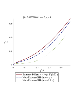
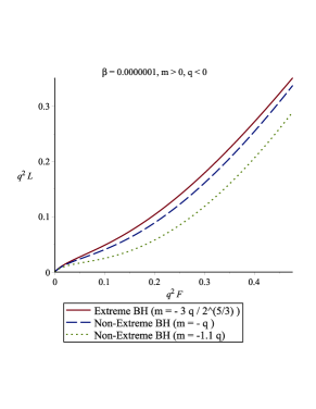
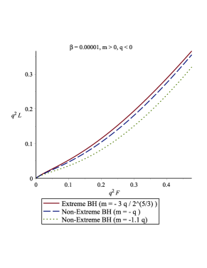
Figure 4: Behavior of $q^{2}\mathcal{L}$ as a function of $q^{2}\mathcal{F}$ for different values of $m/q$.

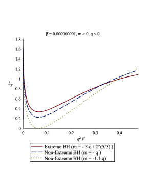
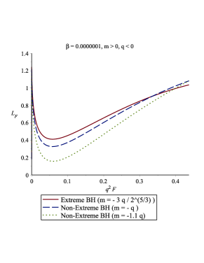
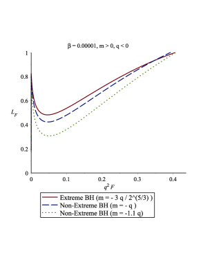
Figure 5: Behavior of $\mathcal{L}_{\mathcal{F}}$ as a function of $q^{2}\mathcal{F}$ for different values of $m/q$.

IV.2 Behavior of the ESTGB-NLED model

In this subsection, we address two particular reductions of the ESTGB-NLED model defined by the functions given in Eqs. (23), (24) and (25), and the behavior of the function $f(\phi)$.

IV.2.1 Reduction to General Relativity

From the following development in power series around $q\approx 0$,

$$\frac{\sqrt{2}\hskip 1.42271ptq^{2}}{\sqrt{qm}}\tan^{\!\!\!{}^{-1}}\!\!\!\left(\!\!\frac{\sqrt{2}\hskip 1.42271ptmr}{q\sqrt{qm}}\!\!\right)=\frac{q^{\frac{3}{2}}\pi}{\sqrt{2m}}-\frac{q^{3}}{mr}+\frac{q^{6}}{6m^{2}r^{3}}-\frac{q^{9}}{20m^{3}r^{5}}+\mathcal{O}\!\left(q^{15}\right),$$ (46)

we see that

$$\frac{\sqrt{2}\hskip 1.42271ptq^{2}}{\sqrt{qm}}\tan^{\!\!\!{}^{-1}}\!\!\!\left(\!\!\frac{\sqrt{2}\hskip 1.42271ptmr}{q\sqrt{qm}}\!\!\right)\Bigg{|}_{q=0}=0.$$

Hence, taking the limit $q\rightarrow 0$ in Eq.(52), we get that $\bm{f}(\phi)=0$ for $q=0$. For the potential $\mathscr{U}$, we have that

$$\lim\limits_{q\rightarrow q_{{}_{0}}}\mathscr{U}\!(r)=\frac{2^{\!{}^{\frac{7}{2}}}\pi m^{\!{}^{\frac{7}{2}}}}{105q^{\!{}^{\frac{11}{2}}}_{{}_{0}}}-\frac{16m^{3}}{105q_{{}_{0}}^{4}r}\!+\!\frac{8m^{2}}{315q_{{}_{0}}r^{3}}\!-\!\frac{16\sqrt{2}m^{4}}{105q_{{}_{0}}^{5}\sqrt{q_{{}_{0}}m}}\!\tan^{\!{}^{\!-1}}\!\!\!\left(\!\!\frac{\sqrt{2}mr}{q_{{}_{0}}\sqrt{q_{{}_{0}}m}}\!\!\right)\!\!,$$ (47)

where we have defined $q_{{}_{0}}=0$. Using (46), it follows that

$$\frac{16\sqrt{2}m^{4}}{105q^{5}_{{}_{0}}\sqrt{q_{{}_{0}}m}}\tan^{\!{}^{\!-1}}\!\!\!\left(\frac{\sqrt{2}\hskip 1.42271ptmr}{q_{{}_{0}}\sqrt{q_{{}_{0}}m}}\right)=\frac{2^{\!{}^{\frac{7}{2}}}\pi m^{\!{}^{\frac{7}{2}}}}{105q^{\frac{11}{2}}_{{}_{0}}}-\frac{16m^{3}}{105q^{4}_{{}_{0}}r}+\frac{8m^{2}}{315q_{{}_{0}}r^{3}}.$$ (48)

Inserting Eq. (48) in Eq.(47), we get $\lim\limits_{q\rightarrow q_{{}_{0}}}\mathscr{U}\!(r)=0$. Proceeding in the same way with Eq.(54),

$$\lim\limits_{q\rightarrow q_{{}_{0}}}2\mathcal{L}(r)\!=\!\frac{16m^{3}}{105q_{{}_{0}}^{4}r}\!-\!\frac{8m^{2}}{315q_{{}_{0}}r^{3}}\!+\!\frac{16\sqrt{2}m^{4}}{105q_{{}_{0}}^{5}\sqrt{q_{{}_{0}}m}}\!\tan^{\!{}^{\!-1}}\!\!\!\left(\!\!\frac{\sqrt{2}mr}{q_{{}_{0}}\sqrt{q_{{}_{0}}m}}\!\!\right)\!-\!\frac{2^{\!{}^{\frac{7}{2}}}\pi m^{\!{}^{\frac{7}{2}}}}{105q^{\frac{11}{2}}}.$$ (49)

Using Eq.(48) we obtain $\lim\limits_{q\rightarrow q_{{}_{0}}}2\mathcal{L}(r)=0$. Thus, we can conclude that when $q=0$, the theory presented here reduces to vacuum GR, and Eq.(29) becomes to the Schwarzschild metric.

IV.2.2 Reduction to a black hole without ADM mass

In the case $m=0$ with $q>0$, the relevant components of the metric given in Eq. (29) are $-g_{tt}=1/g_{rr}=1-q^{3}/r^{3}$. Hence, the event horizon is at $r=r_{h}=q$. The ADM mass of such a solution is null, and its magnetic charge/$\sqrt{2}$ equals its scalar charge, given by $q$. Let us see in detail how the relevant functions that define the theory behave in the zero mass limit. To achieve this goal, we define a quantity $m_{{}_{0}}$, and use the power series expansions of the functions $\bm{f}$, $\mathscr{U}$ and $\mathcal{L}$, for small $m_{0}$, thus obtaining

$$\lim\limits_{m\rightarrow m_{{}_{0}}}\!\!\!\!\bm{f}\!=\!-\frac{r^{3}}{48q}\!-\!\frac{q^{2}r\ln(\beta)}{32m_{{}_{0}}},\hskip 5.69046pt\lim\limits_{m\rightarrow m_{{}_{0}}}\!\!\!\!\mathscr{U}=\!\frac{9q^{5}}{56r^{7}}\!+\!\frac{7q^{8}\ln(\beta)}{48m_{{}_{0}}r^{9}},\hskip 5.69046pt\lim\limits_{m\rightarrow m_{{}_{0}}}\!\!\!\!\mathcal{L}\!=\!-\frac{q^{2}}{4r^{4}}\!-\!\frac{q^{3}}{r^{5}}\!+\!\frac{5q^{5}}{14r^{7}}\!-\!\left(\!\!\frac{3q^{5}}{16m_{{}_{0}}r^{6}}\!-\!\frac{5q^{8}}{24m_{{}_{0}}r^{9}}\!\!\right)\!\ln(\beta).$$ (50)

By direct calculation it can be checked that the model $\bm{f}=-\frac{r^{3}}{48q}-\frac{q^{2}r\ln(\beta)}{32m_{{}_{0}}},$ $\mathscr{U}=\frac{9q^{5}}{56r^{7}}+\frac{7q^{8}\ln(\beta)}{48m_{{}_{0}}r^{9}}$, $\mathcal{L}=-\frac{q^{2}}{4r^{4}}-\frac{q^{3}}{r^{5}}+\frac{5q^{5}}{14r^{7}}-\left(\!\!\frac{3q^{5}}{16m_{{}_{0}}r^{6}}-\frac{5q^{8}}{24m_{{}_{0}}r^{9}}\!\!\right)\!\ln(\beta)$, admits the AF-SSS magnetic massless black hole solution given by $-g_{tt}=1/g_{rr}=1-q^{3}/r^{3}$ for arbitrary values of the parameters ($m_{{}_{0}}$, $\beta$). Hence, we conclude that the divergent terms in (50), i.e., the terms proportional to $1/m_{0}$, cancel out in the ESTGB-NLED field equations. Therefore, these divergent terms can be removed of the theory. Thus, the metric (29), with $m=0$, is a purely magnetic solution of the ESTGB-NLED model determined by;

$$\bm{f}(\phi)=-\frac{q^{2}}{48\phi^{3}}=-\frac{r^{3}}{48q},\hskip 14.22636pt\mathscr{U}(\phi)=\frac{9\phi^{7}}{56q^{2}}=\frac{9q^{5}}{56r^{7}},\hskip 14.22636pt\mathcal{L}(\mathcal{F})=-\frac{\mathcal{F}}{4}\!-\!q^{\frac{1}{2}}\mathcal{F}^{\frac{5}{4}}\!+\!\frac{5q^{\frac{3}{2}}\mathcal{F}^{\frac{7}{4}}}{14}=-\frac{q^{2}}{4r^{4}}\!-\!\frac{q^{3}}{r^{5}}\!+\!\frac{5q^{5}}{14r^{7}}.$$ (51)

From here it is easy to see that $\mathcal{L}(\mathcal{F})$ satisfies the correspondence to Maxwell theory, i.e., $\mathcal{L}\rightarrow-\frac{\mathcal{F}}{4}$, $\mathcal{L}_{\mathcal{F}}\rightarrow-\frac{1}{4}$, as $\mathcal{F}\rightarrow 0$.

V Conclusion

We have derived the first exact solution of the ESTGB-NLED field equations describing an asymptotically flat static and spherically symmetric black hole. The real scalar field constitutes a legitimate hair for the configuration, of the secondary type, since its charge is proportional to the magnetic charge of the black hole. Linear electrodynamics is recovered from the NLED presented here in the limit of sufficiently weak fields.

By requiring that both the effective energy-momentum tensor and that of the NLED satisfy the weak energy condition, we have shown that only values of $q<0$ are allowed. In this case, the solution is akin to the Reissner-Nordström black hole, with the addition of the scalar hair: it can have two horizons, one, or none.

In the limit of zero magnetic charge, the Schwarzschild solution is recovered. Another interesting limit is that achieved when $m=0$, leading to a a solution with magnetic charge (and scalar hair).

It would be of interest to study the stability of these solutions (a good starting point are the developments in Kanti1997 ), as well as the corresponding thermodynamics (following Breton2015 ). We hope to return to these issues in a future publication.

Appendix

In order to describe the limit cases of our solution, it is convenient to write the quantities $\bm{f}(\phi)$, $\mathscr{U}(\phi)$, and $\mathcal{L}(\mathcal{F})$ as functions of the radial coordinate. For the case with $\{m>0,q>0\}$, theses are,

$$\bm{f}\! = \!-\frac{q^{2}}{32m}\!\!\left\{\!\frac{\sqrt{2}\hskip 1.42271ptq^{2}}{\sqrt{qm}}\tan^{\!{}^{\!-1}}\!\!\!\left(\frac{\sqrt{2}\hskip 1.42271ptmr}{q\sqrt{qm}}\right)+\frac{r}{2}\ln\!\!\left[\!\!\left(\!\frac{2m\beta r^{2}}{q^{3}}+\beta\!\right)^{\!\!2}\right]-2r\!\right\}\!\!,$$ (52)

$$\mathscr{U}\!\! = \!\frac{2^{\!{}^{\frac{9}{2}}}\!m^{\!{}^{\frac{7}{2}}}}{105q^{\!{}^{\frac{11}{2}}}}\!\!\left[\!\frac{\pi}{2}\!-\!\tan^{\!{}^{\!-1}}\!\!\!\left(\!\!\frac{\sqrt{2}mr}{q\sqrt{qm}}\!\!\right)\!\right]\!+\!\frac{q^{2}}{4r^{5}}\!\!\left[\!\frac{3m}{10}\!+\!\frac{5q^{3}}{7r^{2}}\!+\!\frac{7q^{6}}{24mr^{4}}\!\right]\!\!\ln\!\!\left[\!\!\left(\!\frac{2m\beta r^{2}}{q^{3}}\!+\!\beta\!\right)^{\!\!2}\right]\!\!-\!\frac{1}{3qr}\!\!\left[\!\frac{16m^{3}}{35q^{3}}\!\!-\!\frac{8m^{2}}{105r^{2}}\!+\!\frac{31mq^{3}}{70r^{4}}\!+\!\frac{11q^{6}}{28r^{6}}\!\right]\!\!,$$ (53)

$$\mathcal{L}\! = \!\frac{q^{2}}{8r^{4}}\!+\!\frac{8m^{3}}{105q^{4}r}\!-\!\frac{4m^{2}}{315qr^{3}}\!-\!\left(\!\frac{37m}{210}\!+\!q\!\right)\!\frac{q^{2}}{r^{5}}\!-\!\frac{5q^{5}}{84r^{7}}\!+\!\frac{2^{\!{}^{\frac{7}{2}}}m^{\!{}^{\frac{7}{2}}}}{105q^{\frac{11}{2}}}\!\!\left[\!\tan^{\!{}^{\!-1}}\!\!\!\left(\!\!\frac{\sqrt{2}mr}{q\sqrt{qm}}\!\!\right)\!-\frac{\pi}{2}\right]$$ (54)

$$\hskip 196.32384pt-\frac{1}{2}\!\left(\!\frac{q^{2}}{8r^{4}}\!-\!\frac{3mq^{2}}{10r^{5}}\!+\!\frac{3q^{5}}{16mr^{6}}\!-\!\frac{4q^{5}}{7r^{7}}\!-\!\frac{5q^{8}}{24mr^{9}}\!\right)\!\ln\!\!\left[\!\!\left(\!\frac{2m\beta r^{2}}{q^{3}}\!+\!\beta\!\right)^{\!\!2}\right]\!\!.$$

Then, by using (9), (29), (52), (53), (54), $\dot{\bm{f}}=\frac{\bm{f}^{\prime}}{\phi^{\prime}}$, $\ddot{\bm{f}}=\frac{1}{\phi^{\prime}}\left(\frac{\bm{f}^{\prime}}{\phi^{\prime}}\right)\!\!^{{}^{{}^{\prime}}}$ and $\mathcal{L}_{\mathcal{F}}=\frac{\mathcal{L}^{\prime}}{\mathcal{F}^{\prime}}$, one finds that the field equations (15), (16), (17), and (18), are satisfied.
For the case with $\{m>0,q<0\}$, rename $q=-Q$ (being $Q>0$), theses are

$$\bm{f}\! = \!-\frac{Q^{2}}{32m}\!\!\left\{\!\frac{Q^{2}}{2\sqrt{2Qm}}\!\ln\!\!\left[\!\!\left(\frac{1+\frac{\sqrt{2}\hskip 1.42271ptmr}{Q\sqrt{Qm}}}{1-\frac{\sqrt{2}\hskip 1.42271ptmr}{Q\sqrt{Qm}}}\!\!\right)^{\!\!\!2}\!\right]+\frac{r}{2}\ln\!\!\left[\!\!\left(\!\frac{2m\beta r^{2}}{Q^{3}}-\beta\!\right)^{\!\!2}\right]-2r\!\right\}\!\!,$$ (55)

$$\mathscr{U}\!\! = \!\!\frac{2^{\!{}^{\frac{5}{2}}}\!m^{\!{}^{\frac{7}{2}}}}{105Q^{\!{}^{\frac{11}{2}}}}\!\ln\!\!\!\left[\!\!\left(\!\!\frac{1\!+\!\frac{\sqrt{2}\hskip 1.42271ptmr}{Q\!\sqrt{Qm}}}{1\!-\!\frac{\sqrt{2}\hskip 1.42271ptmr}{Q\!\sqrt{Qm}}}\!\!\right)^{\!\!\!2}\!\right]\!\!+\!\frac{Q^{2}}{4r^{5}}\!\!\left[\!\frac{3m}{10}\!-\!\frac{5Q^{3}}{7r^{2}}\!+\!\frac{7Q^{6}}{24mr^{4}}\!\right]\!\!\ln\!\!\left[\!\!\left(\!\frac{2m\beta r^{2}}{Q^{3}}\!-\!\beta\!\right)^{\!\!\!2}\right]\!\!-\!\frac{1}{3Qr}\!\!\left[\!\frac{16m^{3}}{35Q^{3}}\!\!+\!\frac{8m^{2}}{105r^{2}}\!+\!\frac{31mQ^{3}}{70r^{4}}\!-\!\frac{11Q^{6}}{28r^{6}}\!\right]\!\!,$$ (56)

$$\mathcal{L}\! = \!\frac{Q^{2}}{8r^{4}}\!+\!\frac{8m^{3}}{105Q^{4}r}\!+\!\frac{4m^{2}}{315Qr^{3}}\!-\!\left(\!\frac{37m}{210}\!-\!Q\!\right)\!\frac{Q^{2}}{r^{5}}\!+\!\frac{5Q^{5}}{84r^{7}}\!-\!\frac{2^{\!{}^{\frac{3}{2}}}m^{\!{}^{\frac{7}{2}}}}{105Q^{\frac{11}{2}}}\!\ln\!\!\!\left[\!\!\left(\!\!\frac{1\!+\!\frac{\sqrt{2}\hskip 1.42271ptmr}{Q\!\sqrt{Qm}}}{1\!-\!\frac{\sqrt{2}\hskip 1.42271ptmr}{Q\!\sqrt{Qm}}}\!\!\right)^{\!\!\!2}\!\right]$$ (57)

$$\hskip 184.9429pt-\frac{1}{2}\!\left(\!\frac{Q^{2}}{8r^{4}}\!-\!\frac{3mQ^{2}}{10r^{5}}\!-\!\frac{3Q^{5}}{16mr^{6}}\!+\!\frac{4Q^{5}}{7r^{7}}\!-\!\frac{5Q^{8}}{24mr^{9}}\!\right)\!\ln\!\!\left[\!\!\left(\!\frac{2m\beta r^{2}}{Q^{3}}\!-\!\beta\!\right)^{\!\!2}\right]\!\!.$$

While for $\{m<0,q>0\}$, rename $m=-M$ (being $M>0$), theses are

$$\bm{f}\! = \!\frac{q^{2}}{32M}\!\!\left\{\!\frac{q^{2}}{2\sqrt{2qM}}\!\ln\!\!\left[\!\!\left(\frac{1+\frac{\sqrt{2}\hskip 1.42271ptMr}{q\sqrt{qM}}}{1-\frac{\sqrt{2}\hskip 1.42271ptMr}{q\sqrt{qM}}}\!\!\right)^{\!\!\!2}\!\right]+\frac{r}{2}\ln\!\!\left[\!\!\left(\!\frac{2M\beta r^{2}}{q^{3}}-\beta\!\right)^{\!\!2}\right]-2r\!\right\}\!\!,$$ (58)

$$\mathscr{U}\!\! = \!\!\frac{2^{\!{}^{\frac{5}{2}}}\!M^{\!{}^{\frac{7}{2}}}}{105q^{\!{}^{\frac{11}{2}}}}\!\ln\!\!\!\left[\!\!\left(\!\!\frac{1\!-\!\frac{\sqrt{2}\hskip 1.42271ptMr}{q\sqrt{qM}}}{1\!+\!\frac{\sqrt{2}\hskip 1.42271ptMr}{q\sqrt{qM}}}\!\!\right)^{\!\!\!2}\!\right]\!\!-\!\frac{q^{2}}{4r^{5}}\!\!\left[\!\frac{3M}{10}\!-\!\frac{5q^{3}}{7r^{2}}\!+\!\frac{7q^{6}}{24Mr^{4}}\!\right]\!\!\ln\!\!\left[\!\!\left(\!\frac{2M\beta r^{2}}{q^{3}}\!-\!\beta\!\right)^{\!\!\!2}\right]\!\!+\!\frac{1}{3qr}\!\!\left[\!\frac{16M^{3}}{35q^{3}}\!\!+\!\frac{8M^{2}}{105r^{2}}\!+\!\frac{31Mq^{3}}{70r^{4}}\!-\!\frac{11q^{6}}{28r^{6}}\!\right]\!\!,$$ (59)

$$\mathcal{L}\! = \!\frac{q^{2}}{8r^{4}}\!-\!\frac{8M^{3}}{105q^{4}r}\!-\!\frac{4M^{2}}{315qr^{3}}\!+\!\left(\!\frac{37M}{210}\!-\!q\!\right)\!\frac{q^{2}}{r^{5}}\!-\!\frac{5q^{5}}{84r^{7}}\!+\!\frac{2^{\!{}^{\frac{3}{2}}}M^{\!{}^{\frac{7}{2}}}}{105q^{\frac{11}{2}}}\!\ln\!\!\!\left[\!\!\left(\!\!\frac{1\!+\!\frac{\sqrt{2}\hskip 1.42271ptMr}{q\sqrt{qM}}}{1\!-\!\frac{\sqrt{2}\hskip 1.42271ptMr}{q\sqrt{qM}}}\!\!\right)^{\!\!\!2}\!\right]$$ (60)

$$\hskip 184.9429pt-\frac{1}{2}\!\left(\!\frac{q^{2}}{8r^{4}}\!+\!\frac{3Mq^{2}}{10r^{5}}\!-\!\frac{3q^{5}}{16Mr^{6}}\!-\!\frac{4q^{5}}{7r^{7}}\!+\!\frac{5q^{8}}{24Mr^{9}}\!\right)\!\ln\!\!\left[\!\!\left(\!\frac{2M\beta r^{2}}{q^{3}}\!-\!\beta\!\right)^{\!\!2}\right]\!\!.$$

Bibliography

Bibliography

(1) Yang, Yingjie and Gong, Yungui, The evidence of cosmic acceleration and observational constraints, JCAP, 06, 059, (2020).
(2) Capozziello, S. and Cardone, V. F. and Troisi, A., Dark energy and dark matter as curvature effects, JCAP 8, 001 (2006).
(3) Fradkin, E.S. and Tseytlin, A.A., Quantum string theory effective action?, Nucl. Phys. B, 261, 1–27 (1985).
(4) Akrami, Y. and others, Planck 2018 results. X. Constraints on inflation, arXiv:1807.06211 (astro-ph.CO), (2018).
(5) D. Doneva, S. Kiorpelidi, P. Nedkova, E. Papantonopoulos, S. Yazadjiev, Charged Gauss-Bonnet black holes with curvature induced scalarization in the extended scalar-tensor theories, Phys. Rev. D 98, 104056 (2018).
(6) S. H. Hendi, M. Momennia, B. Eslam Panah and M. Faizal, Nonsingular Universes in Gauss-Bonnet Gravity’s Rainbow , Astrophys. J. 827, no. 2, 153 (2016).
(7) R.G. Cai, Gauss-Bonnet black holes in AdS spaces , Phys. Rev. D 65, 084014 (2002).
(8) A. Anabalon, N. Deruelle, Y. Morisawa, J. Oliva, M. Sasaki, D. Tempo and R. Troncoso, Kerr-Schild ansatz in Einstein-Gauss-Bonnet gravity: an exact vacuum solution in five dimensions Class. Quant. Grav. 26, 065002 (2009).
(9) I. Antoniadis, E. Gava, and K. S. Narain, Nucl. Phys. B383, 93 (1992), I. Antoniadis, J. Ri zos, and K. Tamvakis, Nucl. Phys. B 415, 497 (1994).
(10) S. Nojiri, S.D. Odintsov, M. Sasaki, Gauss-Bonnet dark energy, Phys. Rev. D 71, 123509 (2005); M. Heydari-Fard, H. Razmi, M. Yousefi, Scalar-Gauss-Bonnet gravity and cosmic acceleration: Comparison with quintessence dark energy, Int. J. Mod. Phys. D 26 1750008 (2017); Koivisto, Tomi and Mota, David F., Cosmology and Astrophysical Constraints of Gauss-Bonnet Dark Energy, Phys. Lett. B, 644, 104-108, (2007); T. Kolvisto, D. Mota, Gauss-Bonnet quintessence: Background evolution, large scale structure, and cosmological constraints, Phys. Rev. D 75, 023518 (2007).
(11) Tsujikawa, Shinji and Sami, M., String-inspired cosmology: Late time transition from scaling matter era to dark energy universe caused by a Gauss-Bonnet coupling, JCAP 01, 006 (2007).
(12) Nojiri, Shin’ichi and Odintsov, Sergei D. and Sami, M., Dark energy cosmology from higher-order, string-inspired gravity and its reconstruction, Phys. Rev. D, 74, 046004, (2006);
Cognola, Guido and Elizalde, Emilio and Nojiri, Shin’ichi and Odintsov, Sergei and Zerbini, Sergio,
String-inspired Gauss-Bonnet gravity reconstructed from the universe expansion history and yielding the transition from matter dominance to dark energy, Phys. Rev. D, 75, 086002, (2007).
(13) Odintsov, S.D. and Oikonomou, V.K. and Fronimos, F.P., Non-Minimally Coupled Einstein Gauss Bonnet Inflation Phenomenology in View of GW170817, Annals Phys. 420, 168250, (2020).
(14)D. Doneva, S. Yazadjiev, New Gauss-Bonnet black holes with curvature induced scalarization in the extended scalar-tensor theories, Phys. Rev. Lett. 120, 131103 (2018).
(15) H. Silva, J. Sakstein, L. Gualtieri, T. Sotiriou, E. Berti, Spontaneous scalarization of black holes and compact stars from a Gauss-Bonnet coupling, Phys. Rev. Lett. 120, 131104 (2018).
(16) J. L. Blázquez-Salcedo, D. D. Doneva, J. Kunz, S. S. Yazadjiev, Radial Perturbations of the scalarized Einstein-Gauss-Bonnet black hole, Phys. Rev. D 98, 084011 (2018); Blázquez-Salcedo, Jose Luis and Doneva, Daniela D. and Kahlen, Sarah and Kunz, Jutta and Nedkova, Petya and Yazadjiev, Stoytcho S., Axial perturbations of the scalarized Einstein-Gauss-Bonnet black holes, Phys. Rev. D 101, 104006, (2020); B. Keihaus, J. Kunz, E. Radu, Rotating Black Holes in Dilatonic-Einstein-Gauss-Bonnet theory, Phys. Rev. Lett. 106, 151104 (2011).
(17)Blázquez-Salcedo, Jose Luis and Doneva, Daniela D. and Kahlen, Sarah and Kunz, Jutta and Nedkova, Petya and Yazadjiev, Stoytcho S., Polar quasinormal modes of the scalarized Einstein-Gauss-Bonnet black holes, Phys. Rev. D 102, 024086 (2020).
(18) Doneva, Daniela D. and Staykov, Kalin V. and Yazadjiev, Stoytcho S., Gauss-Bonnet black holes with a massive scalar field, Phys. Rev. D, 99, 104045 (2019).
(19) P. Kanti, N. E. Mavromatos, J. Rizos, K. Tamvakis, and E. Winstanley, Dilatonic Black Holes in Higher Curvature String Gravity, Phys. Rev. D 54, 5049 (1996).
(20) Doneva, Daniela D. and Staykov, Kalin V. and Yazadjiev, Stoytcho S. and Zheleva, Radostina Z.,
Multi-scalar Gauss-Bonnet gravity – hairy black holes and scalarization, arXiv/gr-qc 2006.11515.
(21) G. Antoniou, A. Bakopoulos, P. Kanti, Evasion of No-Hair Theorems and Novel Black-Hole Solutions in Gauss-Bonnet Theories, Phys. Rev. Lett. 120, 131102 (2018); Black-hole solutions with scalar hair in Einstein-scalar-Gauss-Bonnet theories, Phys. Rev. D 97, 084037 (2018).
(22) G. Antoniou, A. Bakopoulos, P. Kanti, Black hole solutions with scalar hair in the Einstein-scalar-Gauss-Bonnet theories, Phys. Rev. D 97, 084037 (2018); A. Bakopoulos, G. Antoniou, P. Kanti, Novel Black-Hole Solutions in Einstein-Scalar-Gauss-Bonnet Theories with a Cosmological Constant, Phys. Rev. D 99, 064003 (2019).
(23) A. Bakopoulos, P. Kanti, N. Pappas, Large and Ultra-compact Gauss-Bonnet Black Holes with a Self-interacting Scalar Field, Phys. Rev. D 101, 084059 (2020).
(24) M. Born and L. Infeld, Foundations of a new field theory, Proc. Roy. Soc. A 144, 125 (1934).
(25)J. F. Plebański, Lectures on Non-linear Electrodynamics,(NORDITA, Copenhagen, 1970); H. Salazar, A. García, and J. F. Plebański, Duality rotations and type D solutions to Einstein equations with nonlinear electrodynamics sources, J. Math. Phys. 28, 2171 (1987).
(26) Fradkin, E.S. and Tseytlin, Arkady A., Nonlinear Electrodynamics from Quantized Strings, Phys. Lett. B 163, 123–130 (1985).
(27) Gibbons, G.W. and Herdeiro, C.A.R., Born-Infeld theory and stringy causality, Phys. Rev. D 63,064006 (2001).
(28) W. Heisenberg y H. Euler: Folgerungen aus der Diracschen Theorie des Positrons. Z. Phys 98 (1936) 714-732.
(29) M. Aaboud et al. (ATLAS Collaboration), Evidence for light-by-light scattering in heavy-ion collisions with the ATLAS detector at the LHC, arXiv:1702.01625. Published in Nature Physics (2017).
(30) E. Ayón-Beato and A. García, Regular black hole in General Relativity coupled to nonlinear electrodynamics, Phys. Rev. Lett. 80, 5056 (1998); K. A. Bronnikov, Regular Magnetic Black Holes and Monopoles from Nonlinear Electrodynamics, Phys. Rev. D 63, 044005 (2001);77]; E. Ayón-Beato and A. García, Four-parametric regular black hole solution, Gen. Relativ. Gravit. 37, 635 (2005);
(31) K. A. Bronnikov, Nonlinear electrodynamics, regular black holes and wormholes, Int. J. Modern Phys. D, 27, 1841005 (2018); A. V. B. Arellano, F. S. N. Lobo, Evolving wormhole geometries within nonlinear electrodynamics, Class. Quant. Grav. 23 (2006) 5811-5824; S. H. Hendi, Wormhole Solutions in the Presence of Nonlinear Maxwell Field, Advances in High Energy Physics, 697863, (2014); P. Cañate, N. Breton, Black Hole-Wormhole transition in Einstein-anti-de Sitter Gravity Coupled to Nonlinear
Electrodynamics, Phys. Rev. D 98 104012 (2018); P. Cañate, D. Magos, N. Breton, Nonlinear electrodynamics generalization of the rotating BTZ black hole, Phys. Rev. D 101 064010 (2020).
(32) Baldovin, F. and Novello, M. and Perez Bergliaffa, Santiago E. and Salim, J.M., A Nongravitational wormhole”, Class. Quant. Grav. 17, 3265–3276 (2000).
(33) Falciano, F.T. and Peñafiel, M.L. and Perez Bergliaffa, Santiago Esteban,
Entropy bounds and nonlinear electrodynamics, Phys. Rev. D, 100, 125008 (2019).
(34) P. Cañate, J. Sultana and D. Kazanas, Ellis wormhole without a phantom scalar field, Phys. Rev. D 100 (2019) 064007.
(35) P. Cañate and N. Breton, New exact traversable wormhole solution to the Einstein-scalar-Gauss-Bonnet equations coupled to power-Maxwell electrodynamics, Phys. Rev. D 100 (2019) 064067.
(36) H. Stephani, D. Kramer, M. MacCallum, C. Honselaers, and E. Herlt, Exact solutions to Einstein’s Field Equations, Second Edition, Cambridge University Press, Cambridge, U.K., 2003.
(37) Mann, Robert B., Black holes of negative mass, Class. Quant. Grav. 14,
2927–2930 (1997).
(38) Martinez, Cristian, Staforelli, Juan Pablo, and Troncoso, Ricardo, Topological black holes dressed with a conformally coupled scalar field and electric charge, Phys. Rev. D, 74, 044028, 2006.
(39) Garcia, Nadiezhda Montelongo and Harko, Tiberiu and Lobo, Francisco S.N. and Mimoso, Jose P.,
Energy conditions in modified Gauss-Bonnet gravity, Phys. Rev. D 83, 104032 (2011).
(40) Kanti, P. and Mavromatos, N.E. and Rizos, J. and Tamvakis, K. and Winstanley, E., Dilatonic black holes in higher curvature string gravity. 2: Linear stability, Phys. Rev. D 57, 6255–6264 (1998).
(41) Bretón, Nora and Perez Bergliaffa, Santiago Esteban, On the thermodynamical stability of black holes in nonlinear electrodynamics, Annals Phys. 354, 440–453 (2015).