Study of quantum Otto heat engine using driven-dissipative Schrödinger equation

Abstract

The quantum heat engines have drawn much attention due to miniaturization of devices recently. We study the dynamics of the quantum Otto heat engine using the driven-dissipative Schrödinger equation. Starting from different initial states, we simulate the time evolutions of the internal energy, power and heat-work conversion efficiency. The initial state impacts on these thermodynamic quantities before the Otto cycle reaches stable. In the transition period, the efficiency and power may be higher or lower than the corresponding values in the cyclostationary state. Remarkably, the efficiency could surpass the Otto limit and even the Carnot limit and the power could be much higher than the rated power. The efficiency anomaly is due to the energy in the initial state. Thus, we suggest that periodically pumping could take the similar role of a hot bath but could be manipulated flexibly. Furthermore, we propose a new quantum engine working in a single reservoir to convert the pump energy into mechanical work. This manipulative engine could potentially be applied to working in the microenvironments without a large temperature difference, such as the biological tissues in vivo. Our protocol is expected to model a new quantum engine with the advantage of applicability and controllability.

I introduction

Converting heat into mechanical work periodically, the heat engines as the generators of motion triggered both the industrial revolution and the theoretical development of thermodynamics in the $18$th and $19$th centuries. Recently, the heat engines have been re-invigorated by miniaturization of devices Hänggi and Marchesoni (2009). Experimentally, elaborate efforts have been made on the design of the machines employing quantum systems, such as harmonic oscillators Lin and Chen (2003), ultracold atoms Brantut et al. (2013), a single particle, such as an atom, ion, electron Abah et al. (2012); Koski et al. (2014); Rana et al. (2014); Roßnagel et al. (2016); von Lindenfels et al. (2019) and molecular Hill et al. (2005) as well as a spin-1/2 system Geva and Kosloff (1992); Thomas and Johal (2011); von Lindenfels et al. (2019); Peterson et al. (2019) and qubit system Linden et al. (2010); Brunner et al. (2012); Brask et al. (2015). They work at the atom level to convert heat or light into mechanical or electrical power Benenti et al. (2017); Klaers et al. (2017). Theoretically, various model systems performing thermodynamic cycles have been proposed as the quantum heat engines (QHEs), dating back to the three-level masers proposal in 1959 Scovil and Schulz-DuBois (1959). Recently, more attentions are drawn to the relationship between different types of QHEs Quan et al. (2007); Uzdin et al. (2015); Elouard et al. (2017); Klatzow et al. (2019), irreversible work and inner friction Rezek and Kosloff (2006); Plastina et al. (2014), the impact of coherence Scully et al. (2003); Rahav et al. (2012); Goswami and Harbola (2013) and the application prospects and the transition to refrigerators Gelbwaser-Klimovsky et al. (2013); Kosloff and Levy (2014); Uzdin and Kosloff (2014); Hofer et al. (2016); Camati et al. (2020). These QHEs not only comply with the classical laws of thermodynamics but also follow the rules of quantum mechanics Quan et al. (2005); Kosloff (2013); Skrzypczyk et al. (2014). Consequently, the quantum thermodynamics is boosted by engineering a variety of quantum devices.

Among the QHEs, the quantum Otto heat engine (QOHE), mimicking the common four-strokes car engine, has been extensively studied Feldmann and Kosloff (2003); Kieu (2004); Hübner et al. (2014); Roßnagel et al. (2014); Kosloff and Rezek (2017); Watanabe et al. (2017); Camati et al. (2019); Das and Mukherjee (2020); Wiedmann et al. (2020). The working substance is only a quantum harmonic oscillator with a tunable vibration frequency. The heat engine is alternately coupled to a hot and a cold reservoir. The $4$-stroke Otto cycle consists of two isochoric processes and two adiabatic processes. During the isochoric processes, the QOHE exchanges heat with the hot or cold baths but keeps the frequency constant. In the adiabatic processes, the work input or output changes the frequency of the oscillator.

In this paper, we take advantage of the driven-dissipative Schrödinger equation to study the time evolution of the quantum Otto cycle process and evaluate the performance of QOHE. The time-dependent probability distribution of the oscillator’s energy levels is calculated by the driven-dissipative Schrödinger equation. The time evolutions of the internal energy, power and efficiency are simulated. The quantum machine starts from the ground state, the coherent state and the state with equal probability distribution on several lower energy levels, respectively. In the first case, the efficiency and power increase with the number of the Otto cycles until they reach a stable value. In the latter two cases, the efficiency could be larger than the Otto limit, or even the Carnot limit, and the power could be much higher than the rated power. The overrange is due to the contribution of the energy stored in the initial state. It implies an effective method to manipulate the QOHE. Thus, we suggest that periodically pumping quantum heat engine could enhance the rated power and also could substitute the role of a hot bath. Therefore, we propose a possible design of a new quantum engine working in a single bath to convert the pump energy into the mechanical work. Such an engine may be used for working under control in the microenvironments. We also study the balance between the net power output and the machine efficiency since it is impossible to realize the maximums of both the efficiency and power output at the same time.

II Model of quantum Otto heat engine

We apply the driven-dissipative Schrödinger equation Chang et al. (2010); van Veenendaal et al. (2010) to study the time evolution of the QOHE. The energy exchange between the QOHE and the heat reservoirs is described by the driven-dissipative operator $D$. Previously, we call it the dissipative operator in the decaying process Chang et al. (2010); van Veenendaal et al. (2010). This equation could deal with strong system-environment coupling and the substantial environmental memory effects, as demonstrated in our previous work Chang et al. (2012). The dissipative Schrödinger equation with the time-dependent quantum state is written as

$$i\hbar\frac{d\left|\psi\left(t\right)\right\rangle}{dt}=\left(H_{0}+iD\right)\left|\psi\left(t\right)\right\rangle,$$ (1)

where the Hamiltonian $H_{0}$ of the quantum harmonic oscillator with a time-dependent frequency reads

$$H_{0}=\hbar\omega\left(t\right)a^{\dagger}a,$$ (2)

where $a^{\dagger}$ and $a$ are the Bosonic creation and annihilation operators. Alternatively,

$$H_{0}=\underset{n}{\sum}E_{n}\left|n\right\rangle\left\langle n\right|,$$ (3)

where the energy of the ground state $\left|0\right\rangle$ is assumed to be zero, $\left|n\right\rangle$ is the $n$-bosons state of the oscillator, and the corresponding energy $E_{n}=n\hbar\omega$.

Selecting $\left|n\right\rangle$ as the basis, we write the system wave vector

$$|\psi(t)\rangle=\sum_{n}c_{n}(t)|n\rangle,$$ (4)

with the coefficient $c_{n}$ in terms of an amplitude $a_{n}(t)=|c_{n}(t)|$ and a phase $\varphi_{n}(t)$, or $c_{n}(t)=a_{n}(t)e^{i\varphi_{n}(t)}$. We can express the change in the coefficient due to the presence of the bath

$$\left.\frac{dc_{n}(t)}{dt}\right|_{B}=\left.\frac{da_{n}(t)}{dt}\right|_{B}e^{i\varphi_{n}(t)}+i\left.a_{n}(t)e^{i\varphi_{n}(t)}\frac{d{\varphi_{n}(t)}}{dt}\right|_{B}.$$ (5)

In general, the coupling to the environment affects both the probability and the phase of the system. The latter term gives the change in phase induced by its surroundings. Due to the complexity of the surroundings, its nature usually only is taken into account in an effective way. Here, we assume that the phase of the local system is changed randomly by the large number of degrees of freedom of the surroundings which results in a total phase change close to zero or a constant according to the law of large numbers. We therefore only consider the changes in the probability by the environment. Below we give the explicit expression for the change in probabilities $P_{n}(t)=a_{n}^{2}(t)$. The change in the coefficient due to the bath is then given by

$$\left.\frac{dc_{n}(t)}{dt}\right|_{B}=\frac{1}{2a_{n}(t)}\left.\frac{dP_{n}(t)}{dt}\right|_{B}e^{i\varphi_{n}(t)}=\left.\frac{1}{2}\frac{d\ln P_{n}(t)}{dt}\right|_{B}c_{n}(t).$$ (6)

This leads to the $D$ operator describes the state changes of the system by surroundings, which is given by

$$D=\frac{\hbar}{2}\underset{n}{\sum}\frac{d\ln P_{n}\left(t\right)}{dt}\left|n\right\rangle\left\langle n\right|.$$ (7)

The time evolution of the probability distribution function $P_{n}\left(t\right)$ of the $n$th state is described by the rate equation Chang et al. (2010)

$$\frac{dP_{n}\left(t\right)}{dt} =-2n\Gamma P_{n}\left(t\right)+2\left(n+1\right)\Gamma P_{n+1}\left(t\right)$$

$$\ -2\Gamma e^{-\hbar\omega/k_{B}T}\left[-nP_{n-1}\left(t\right)+\left(n+1\right)P_{n}\left(t\right)\right],$$ (8)

where $\Gamma=\Gamma_{0}(n_{BE}+1)$ with the Bose-Einstein distribution $n_{BE}$ and the relaxation constant $\Gamma_{0}$ of the oscillator induced by the reservoirs. The factor $e^{-\hbar\omega/k_{B}T}$ is introduced to ensure the rate equation obeying the usual detailed balance relations. The first two terms at the right side of Eq. (8) describe the change of $P_{n}$ due to emitting a boson to the bath, and the other two terms for the change of $P_{n}$ due to absorbing a boson from the bath.

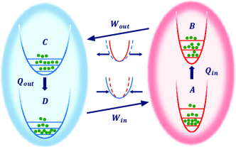
Figure 1: Schematic cycle of the quantum Otto heat engine mimicking a classical $4$-cycle engine. The cycle includes two isochoric processes ($A\rightarrow B,\ C\rightarrow D$) and two adiabatic processes ($B\rightarrow C,\ D\rightarrow A$). In the isochoric phases, the oscillator absorbs the heat $Q_{in}$ from the hot bath with the temperature $T_{h}$ and releases the heat $Q_{out}$ to the cold bath with the temperature $T_{c}$, respectively. In the adiabatic phases without entropy change, the work output $W_{out}$ and work input $W_{in}$ induce the decrease and increase of the oscillator frequency, respectively. The horizontal line segments in the parabolic curves represent the energy levels of the oscillator and the bottom horizontal line indicates the ground state.

Starting from a given initial population distribution $P_{n}(t=0),$ we solve the driven-dissipative Schrödinger equation and obtain the temporal variation of $P_{n}(t)$. Thus, the time-dependent internal energy of the QOHE reads

$$U(t)=\underset{n}{\sum}E_{n}P_{n}(t).$$ (9)

The internal energy of the engine may be changed by the work output or input as well as the exchange heat with a bath. According to the first law of thermodynamics $\mkern 3.0mu\mathchar 22\relax\mkern-12.0mudU=\mkern 3.0mu\mathchar 22\relax\mkern-12.0mudQ+\mkern 3.0mu\mathchar 22\relax\mkern-12.0mudW$, then Kieu (2004, 2006)

$$\mkern 3.0mu\mathchar 22\relax\mkern-12.0mudQ=\underset{n}{\sum}E_{n}dP_{n};\ \mkern 3.0mu\mathchar 22\relax\mkern-12.0mudW=\underset{n}{\sum}P_{n}dE_{n}.$$ (10)

During the thermal cycle, the occupation probability apportion $P_{n}$ of the $n$-bosons state changes in the endothermic and exothermic processes, and keeps constant in the adiabatic processes. If there are no coherence in the $\left|n\right\rangle$ states, the von Neumann entropy $S(t)$ as function of occupation distribution $P_{n}(t)$ is written as

$$S(t)=-k_{B}\underset{n}{\sum}P_{n}(t)lnP_{n}(t),$$ (11)

where $k_{B}$ is the Boltzmann constant.

Let address the $4$-stroke Otto cycle in more detail. In the isochoric processes, the heat exchange with the heat reservoirs changes the particle occupation allocation $P_{n}(t)$ without work done or $\mkern 3.0mu\mathchar 22\relax\mkern-12.0mudW=0$, i.e., in the stages $A\rightarrow B$ and $C\rightarrow D$, as shown in Fig. 1. In the adiabatic or isentropic processes, the oscillator frequency of the QHE changes slowly with time to ensure that there is no change of the particle occupation on each level or $dP_{n}=0$, and then the entropy $S(t)$ keeps a constant. There is also no heat exchange with the heat reservoirs or $\mkern 3.0mu\mathchar 22\relax\mkern-12.0mudQ=0$, i.e., in the stages $B\rightarrow C$ and $D\rightarrow A$.

$A\rightarrow B$: starting from an initial state at the point $A$, the QOHE contacts the hot bath with the temperature $T_{h}$. The oscillator is heated up by the hot bath and keeps its frequency $\omega_{h}$ constant. To the point $B$, it stops exchanging heat with the hot bath. The total absorbed heat is

$$Q_{in}=\underset{n}{\sum}n\hbar\omega_{h}\left(P_{n}^{B}-P_{n}^{A}\right).$$ (12)

$B\rightarrow C$: the machine does work in adiabatic expansion step. The von Neumann entropy remains unchanged, $dP_{n}=0$ or $P_{n}^{C}=P_{n}^{B}$. The oscillation frequency relaxes from $\omega_{h}$ to $\omega_{c}$, and the work output is

$$W_{out}=\sum_{n}n\hbar\left(\omega_{h}P_{n}^{B}-\omega_{c}P_{n}^{C}\right).$$ (13)

$C\rightarrow D$: the heat engine couples to the cold bath at the temperature $T_{c}$. The QOHE keeps the same frequency $\omega_{c}$ and releases the heat $Q_{out}$ to the cold bath with

$$Q_{out}=\underset{n}{\sum}n\hbar\omega_{c}\left(P_{n}^{C}-P_{n}^{D}\right).$$ (14)

$D\rightarrow A^{\prime}$: the adiabatic compression starts and the frequency of the oscillator is enhanced from $\omega_{c}$ to $\omega_{h}$ by the input work

$$W_{in}=\sum_{n}n\hbar\left(\omega_{h}P_{n}^{A^{\prime}}-\omega_{c}P_{n}^{D}\right),$$ (15)

with $P_{n}^{A^{\prime}}=P_{n}^{D}$. It is worthy of noting that the $P_{n}^{A^{\prime}}$ is not always equal to the $P_{n}^{A}$ unless the Otto cycle is periodically stable.

The effective or net work output $W_{eff}$ throughout the Otto cycle is given by

$$W_{eff}=W_{out}-W_{in}.$$ (16)

Substituting the Eqs. (13) and (15) into Eq. (16), the total effective work $W_{eff}$ done per Otto cycle is written as

$$W_{eff}=\sum_{n}n\hbar\left[\left(\omega_{h}P_{n}^{B}-\omega_{c}P_{n}^{C}\right)-\left(\omega_{h}P_{n}^{A^{\prime}}-\omega_{c}P_{n}^{D}\right)\right].$$ (17)

Applying the conventional definition, the heat-work conversion efficiency $\eta$ for the QOHE is given by

$$\eta=\frac{W_{eff}}{Q_{in}}.$$ (18)

Combining Eq. (17) and (12), the efficiency $\eta$ is rewritten as

$$\eta=\frac{\underset{n}{\sum}n\hbar\left[\omega_{h}\left(P_{n}^{B}-P_{n}^{A^{\prime}}\right)-\omega_{c}\left(P_{n}^{C}-P_{n}^{D}\right)\right]}{\underset{n}{\sum}n\hbar\omega_{h}\left(P_{n}^{B}-P_{n}^{A}\right)}.$$ (19)

We assume the frequency of the oscillator changes slowly enough in the expansion and compression process with no population redistribution or without inner friction Rezek (2010); Camati et al. (2019); Plastina et al. (2014). One has $P_{n}^{B}=P_{n}^{C},\ P_{n}^{D}=P_{n}^{A^{\prime}}$. Then, the efficiency $\eta$ can be obtained by simplifying Eq. (19) as

$$\eta=\eta_{O}\frac{\underset{n}{\sum}n\left(P_{n}^{B}-P_{n}^{A^{\prime}}\right)}{\underset{n}{\sum}n\left(P_{n}^{B}-P_{n}^{A}\right)},$$ (20)

with the Otto efficiency $\eta_{O}=1-\omega_{c}/\omega_{h}$.

It is worthy of noting that in the efficiency definition, the contribution of energy in the initial state is ignored. $P_{n}^{A}$ could be very different to $P_{n}^{A^{\prime}}$ or the value in the stable cycles when the machine is away from a stable cycle, which could lead to the efficiency strongly deviated from the Otto limit. For example, starting from a high energy state, the machine even releases heat into the hot bath or $Q_{in}<0$, and then the efficiency becomes negative. In particular, if we prepare the stating state with $P_{n}^{A}=P_{n}^{B}$, we even get the divergence of the efficiency. In the following, we show that if the energy in the initials state is taken into account, the maximum of the efficiency is still the Otto limit.

III Time evolution of quantum Otto heat engine

A. Otto Cycle without formation of thermal balance

In this section, we simulate the time evolution process of the $4$-stroke Otto cycle without formation of thermal balance with the baths. Each period includes four same time segments, e.g., $\tau=\tau_{AB}=\tau_{BC}=\tau_{CD}=\tau_{DA}$.

In all the numerical calculations, we set the lower oscillator energy $\hbar\omega_{c}$ as the energy unit, and $\tau_{c}=2\pi/\omega_{c}$ as the time unit.

During the working stroke, the oscillator frequency reducing or increasing is similar to the volume expanding or compressing in the classical model. We set the time evolution of the frequency function as $\omega\left(t\right)=\omega_{h,c}-t(\omega_{h,c}-\omega_{c,h})/\tau$. The harmonic frequency gradually decreases from $\omega_{h}$ to $\omega_{c}$ during the time $\tau_{BC}$ in the work output stages and gradually increases from $\omega_{c}$ to $\omega_{h}$ during the time $\tau_{DA}$ in the work input stages. These working strokes take place under adiabatic conditions, and no heat exchange with heat reservoirs or $\mkern 3.0mu\mathchar 22\relax\mkern-12.0mudQ=0$. During the thermal exchanging stroke, the vibration frequency is kept constant, and the oscillator exchanges heat with the reservoir without work done or $\mkern 3.0mu\mathchar 22\relax\mkern-12.0mudW=0$.

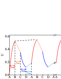
Figure 2: The time evolutions of the internal energy $U$ in the QOHE starting from the ground state to the periodic steady state. The red and blue solid lines indicate the two isochoric processes in the duration $\tau_{AB}$ and $\tau_{CD}$. The orange and light-blue dashed lines indicate the two adiabatic processes with the constant entropies in the segments $\tau_{BC}$ and $\tau_{DA}$. In our numerical calculations, we set $\hbar\omega_{c}$ as the unit of energy, and $\tau_{c}=2\pi/\omega_{c}$ as the unit of time. The working duration $\tau=2.0$. The harmonic oscillators of low frequency $\hbar\omega_{c}=1.0$ and high frequency $\hbar\omega_{h}=1.5$. The temperature of cold bath $k_{B}T_{c}=0.4$ and the temperature of the hot bath $k_{B}T_{h}=1.2$, respectively. Here, we define the relaxation time constant between the oscillator and the reservoirs $\left(2\Gamma_{0}\right)^{-1}=1$. The right side of the separator shows the results when the Otto cycle reaches a periodical stable state. The top black oblique dashed line indicates that the difference of the internal energy $U$ at the points $B$ and $B^{\prime}$ before the machine reaches a stable state.

The time evolution of the internal energy $U$ and efficiency $\eta$ depend on the time-dependent probabilities of the oscillator’s energy levels. The occupancy distribution is determined by solving the driven-dissipative Schrödinger equation.

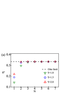
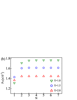
Figure 3: The efficiency $\eta$ (a) and power $P_{W}$ (b) versus the number $N$ of the Otto cycles starting from the ground state. The single-segment time $\tau$ takes $1.0$, $1.5$ and $2.0$. The temperature and frequency parameters are the same as those in Fig. 2. The power is expressed in relative unit of energy and time.

Firstly, we set the ground state of the oscillator as the initial state. The time evolution of the internal energy $U$ is shown in Fig. 2. The thermal engine reaches cyclostationary state after several periods. With the number $N$ of the Otto cycle increasing, the quantum machine gradually approaches periodically steady. For instance, the number of particles on each state reach constant values at points $A$, $B$, $C$, $D$, as shown the right of the separator in Fig. 2. In addition, we obtain the evolution of efficiency at different working duration $\tau$ as the illustration in Fig. 3(a). The Otto engine reaches periodic stability after several cycles. The longer the evolution time lasts, the closer $P_{n}^{A}$ is to $P_{n}^{A^{\prime}}$, which means that the efficiency $\eta$ is approaching $\eta_{O}$, see Eq. (20). In the non-steady cycle, the longer the working duration $\tau$ is, the higher the efficiency $\eta$ is. Because the QOHE starts from the ground state, $Q_{in}$ in the first-stroke is much larger than that in subsequent cycles. Consequently, the efficiency is lower than the Otto limit in the first stage. The efficiency $\eta$ of the QOHE could reach a stable value after several cycles. It is worth noting that $P_{n}^{A^{\prime}}=P_{n}^{A}$ holds only when the Otto cycle reaches a steady cyclical state and the efficiency $\eta$ in Eq. (20) reaches the Otto limit $\eta_{O}$. On the other hand, as long as the probability of $P_{n}^{A}$ is different from $P_{n}^{A^{\prime}}$, the efficiency deviates from the Otto limit $\eta_{O}$.

The power output $P_{W}$ is another indicator to judge the performance of the QOHE. It could be expressed as

$$P_{W}=W_{eff}/4\tau,$$ (21)

where $4\tau$ is total time of an Otto cycle. The time evolution of power is illustrated in Fig. 3(b). During the initial several cycles, the power is lower than the value in the stable cyclic state. The working substance does not warm up to the optimal working order in the beginning few cycles. The power is also lower according to the Eqs. (16) and (21). The power reaches the maximum as long as the cycle reaches a fixed periodic state. In addition, the shorter the working cycle duration is, the higher the output power is at the regular stable states, which is similar to that of classic heat engines.

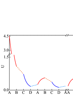
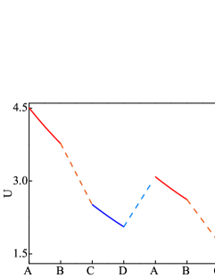
Figure 4: The time evolutions of the energy $U$ (a) starting from a initial state with the equal probability distribution on the lower three energy levels. The energy $U$ (b) and (c) as the function of the time starting from the coherent state, and the relaxation time $(2\Gamma_{0})^{-1}$ in the latter is ten times longer than that in the former to slow down the decoherence by environments. The parameters of temperature $T_{c,h}$, frequency $\omega_{c,h}$ and the duration of single-stroke $\tau$ are the same as those in previous case starting from the ground state. The red and blue solid lines represent endothermic and exothermic strokes, respectively. The orange and light-blue dashed lines represent the adiabatic working strokes.

Secondly, we set the initial state with the equal probability distribution on the three lower energy levels of the oscillator. All the other parameters such as the temperatures and frequencies are the same as the previous case. The energy of this initial state is much higher than that in the case starting from the ground state. On account of the speedy redistribution of the probabilities among the high energy levels in the initial stage, the energy quickly decays at the beginning of the evolution and gradually tends to a periodic stabilization, as shown in Fig. 4(a). In the starting periods, the energy of the QOHE even releases into the hot bath in the form of heat during the $\tau_{AB}$ or $Q_{in}<0$.

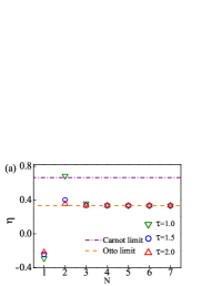
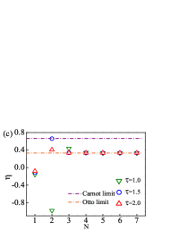
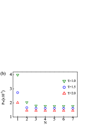
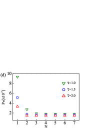
Figure 5: The efficiency $\eta$ (a) and power $P_{W}$ (b) versus the number of cycles $N$ with the equal probability distribution on the three lower energy levels as the initial state. The efficiency $\eta$ (c) and power $P_{W}$ (d) versus the number of cycles $N$ starting from the coherent state. The single-segment time $\tau$ takes different values. The temperature and frequency parameters are the same as those in Fig. 2, respectively.

Fig. 5(a) shows the time evolution of the efficiency. In the beginning stages, one finds the negative efficiency value due to the negative $Q_{in}$ and hence negative efficiency $\eta=W_{eff}/Q_{in}$. The $Q_{in}$ gradually approaches zero and then becomes positive. It is worth noting that in the $2$nd period, the efficiency even exceed the Carnot or Otto limit. This does not means that the thermodynamic laws are violated, and it is attributed to the contribution from the energy stored in the initial state. Consequently, it provides a route to improve the manipulations of the QOHE by external control, for example, populating the high levels of the QHE by light or vibration pump. In the stable periodic state of the QOHE, the efficiency returns to the Otto limit $\eta_{O}$. The diagram of power evolution is shown in Fig. 5(b). The power decays from a higher value to a constant. As the Otto cycle approaches a cyclostationary state, the time evolutions of $U$, $\eta$ and $P_{W}$ are all the same as those starting from the ground state.

The enhancement of power by pumping potentially is of importance in realistic applications. For example, in a given environment, a heat engine works with rated power. If we come across a local obstacle that need larger power, then we need a substitute of the working engine. With the light or vibration pump, we could enhance the power beyond the rated power of the engine without replacing the engine.

Finally, we start from the coherent state with the occupation probability following the function $P_{n}\sim e^{-\left[\left(n-n{{}^{\prime}}\right){\hbar\omega/k_{B}T}\right]^{2}}$ with $n$ for $n$th energy level and $n{{}^{\prime}}$ for the central level. However, once system-bath interaction is turned on, coherence loses quickly. The heat machine reaches a thermal equilibrium state within several cycles. The time evolution of the internal energy, efficiency and power is similar to those starting from the initial state with the equal probability distribution on the three lower energy levels, as shown in Fig. 4(b) and Fig. 5(c, d). To slow down the environment induced decoherence, we prolong the relaxation time $(2\Gamma_{0})^{-1}$ ten times longer, then the deformation of the wave packet with time could be reduced and the coherent state is more like a state of a classical oscillator at the beginning of the evolution. The energy increases or decreases almost linearly, as shown in the Fig. 4(c). The efficiency and power are strongly reduced (not shown).

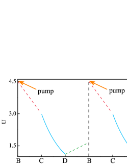
Figure 6: The time evolution of the energy $U$ under periodically pumping in a single heat reservoir. First energy level excited state (a) and coherent state (b). Here, single-stage duration $\tau=1.0$ and the thermal source at fixed $k_{B}T_{c}=0.4$. The frequencies of harmonic oscillators are the same as the previous cases. The red and green dashed lines show the segments of isentropic working; the light-blue solid lines show the segments of isochoric heat release. The pumping operation is performed at the beginning of each cycle as indicated by the orange arrows in all pictures. The pump duration $\tau_{AB}$ is ignored for it is much shorter than $\tau$.

B. QHE with Single-bath

Heat engine always operates in two heat reservoirs. However, two baths with different temperature are difficult to realize in microenvironments, such as organism and nanostructures. Since the initial state affects the time evolution of the power, internal energy and the efficiency at least in the early QHE cycles, we could periodically pump the QHE and operate it more easily. Therefore, here, we propose to pump the quantum engine with a light or vibration pump and convert the pump energy into the mechanical work in a single heat reservoir or in a normal temperature environment. In other words, the energy provided by pump substitutes the heat absorption from the hot bath in the Otto cycles, and then the quantum engine operates in a single heat bath with the temperature $T_{c}$. The engine is regularly pumped at the beginning of the cycles to initialize the occupation probability distribution. Since the pump duration $\tau_{AB}$ is extremely short, comparing with the time segments of $\tau_{BC}$, $\tau_{CD}$ and $\tau_{DB}$, we neglect $\tau_{AB}$ in our figures in this model. The evolution process of the internal energy is shown in Fig. 6(a). The QOHE is periodically pumped from the ground state to the first excited state at beginning of each cycle with the pump energy $Q_{pump}$. This engine actually converts the pump energy into heat and mechanical work. The heat release process is necessary because the pump energy is impossible to be converted into work completely without the heat dissipation according to the second law of thermodynamics. During the adiabatic strokes, the processes of the work input and output are similar to the compression and expansion of classical heat engine. The Otto cycle can be redivided into four processes: pump, expansion, heat release and compression. The efficiency is redefined as the ratio of the net work output to the pump energy, i.e., $\eta=\left(W_{out}+W_{in}\right)/Q_{pump}$.

Actually, the pump method could easily prepare variants of initial states. We set the coherent state as the initial state to start engine. The internal energy as a function of the working time is illustrated in Fig. 6(b). The time evolution is similar to that of the first level excited state. In Fig. 7, starting from the coherent state, one finds that the efficiency is significantly improved comparing with the case starting from the first level excited state, . Since coherence plays an important role in improving the performance of QHEs Camati et al. (2020); Guff et al. (2019); Dodonov et al. (2018), we further study the state coherence effects. The quantum coherence is weakened as the system interacting with environments Gong and Brumer (2003). The longer the time lasts, the less coherence is left and the less input work is needed to start the next cycle. In this pump-driven machine, the system environment interaction takes place only in the heat exchange phase $\tau_{CD}$. We study the efficiency as the function of the time variable $\tau_{CD}$. In Fig. 7(a), the efficiency is improved with the time $\tau_{CD}$ increasing until the time ratio $\tau_{BC}/\tau_{CD}\sim 0.2$, where the efficiency reaches the upper bound. According to the results in Fig. 7(a), the efficiency reaching its maximum implies the thermalization is completely carried out. Another significant factor is the relaxation constant $\Gamma_{0}$, which reflects the speed of relaxation. Here, we set the relaxation time $\left(2\Gamma_{0}\right)^{-1}$ as the variable parameter. As $\left(2\Gamma_{0}\right)^{-1}$ increases, the complete thermalization stroke takes a longer time, and as shown in Fig. 7(b), the efficiency gradually deviates from the Otto limit. Therefore, we could intervene into the initial state by periodic pumping to improve the performance of heat engines.

The pump-driven engine has important potential applications. In microenvironments, such as living organisms and nanostructures, it is almost impossible to provide two baths with large temperature difference. The single bath engine driven by light pumping outside is a quite suitable candidate to work in microenvironments. For instance, under the controllable light irradiation, atomic dimers, quantum dots or magnetic clusters absorb photons and then the chemical bonds prolong and perform mechanical motion Hübner et al. (2014); Benenti et al. (2017). Equipped with this kind of engines, biological machines or molecule cars could be used to identify and destroy lesions Novotný et al. (2020). For example, to purge the clots in blood vessel, a nanorobot could be sent to the location of the clots to deliver drugs or directly dredge the clogged blood vessel. The nanorobot equipped with the pump-driven engine could work under external pumping control without a cable or a battery.

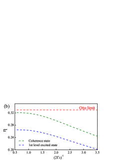
Figure 7: Dependence of efficiency on thermalization time and relaxation time. (a) efficiency vs variant system-environment interaction time $\tau_{CD}$ with the work time $\tau_{BC}=\tau_{DB}=1$, the relaxation time constant $\left(2\Gamma_{0}\right)^{-1}=1$. (b) efficiency vs the relaxation time parameter $\left(2\Gamma_{0}\right)^{-1}$. The time interval for all stages are $\tau_{BC}=\tau_{DB}=1,~{}\tau_{CD}=5$, respectively. The frequencies of harmonic oscillators and temperature are the same as the previous cases.

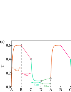
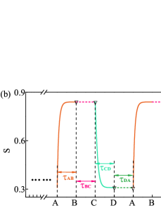
Figure 8: The time evolutions of the energy $U$ (a) with the QOHE reaching thermal balance with the baths. $\hbar\omega_{c}=1.0$ and $\hbar\omega_{h}=1.5$. (b) Entropy evolution diagram after the quantum state coherence disappears completely. We set the working time of single-step $\tau=10.0$. The temperature parameters of cold bath and hot bath are $k_{B}T_{c}=0.4$ and $k_{B}T_{h}=1.2$. The pink and green solid lines display the isochoric heat exchange stages; The orange and light-green dashed lines display the isentropic working stages. The hollow diamond and triangle symbols represent analytical results, exactly locating on the numerically calculated curves.

C. Otto cycle with thermal balance

We have studied the performance of the QOHE without forming thermal equilibrium with the heat baths in the above sections. In the following, we prolong the duration of periodic cycle to make the machine reach the thermal equilibrium with the baths in the heat exchange processes. The harmonic oscillator’s frequency and environmental conditions are exactly the same as those in the previous sections. When the QOHE reaches thermal balance with the heat reservoirs, the population probabilities obey the Boltzmann distribution, $P_{n}\propto e^{-E_{n}/k_{B}T}$. During the heat-exchange processes, the frequencies of the harmonic oscillators remain unchanged. The population distribution function $P_{n}$ at the thermal balance could be calculated analytically. The initial state also starts from the ground state, and the cycle reaches stable in the first stage $\tau_{AB}$. Only in the first cycle, the absorbed heat and efficiency are different from those in the subsequent cycles. The time evolution of the entropy is shown in the Fig. 8(b). Since Eq. (11) fails to apply to the entropy calculation of the states with coherence. We omit the stating stages of the Otto cycles until the coherence completely is eliminated. The orange and light-green dashed lines display the isentropic working stages.

Our numerical calculations of energy and entropy qualitatively agree well with the results obtained by the Lindblad methods Dodonov et al. (2018); Park et al. (2019). In addition, the data points based on analytical calculation at the points $A,\ B,\ C,\ D$ also exactly locate on our numerically calculated curves, as shown in Fig. 8.

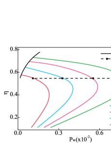
Figure 9: The efficiency $\eta$ versus the effective power output $P_{W}$ of QOHE. Different colored lines represent the relationship between efficiency and net output power at different $T_{h}$ by gradually changing the frequency ratio $\omega_{c}/\omega_{h}$. The cold bath temperature $k_{B}T_{c}=0.4$. The black horizontal dashed line sketches the power $P_{W}$ vs $T_{h}$ at a fixed $\eta$. Black solid line indicates the Carnot limit, constraining the efficiency of the QOHE.

QHEs often fail to maximize both the output power and the efficiency Abah et al. (2012). The balance between the power and efficiency is pursued. We fix the cold bath temperature a constant value, and adjust the hot bath temperature as well as the frequency ratio $\omega_{c}/\omega_{h}$. The relationship between the efficiency versus the output power is shown in Fig. 9. The power versus efficiency shows a quasi-parabolic curve. It is impossible for both of them to reach the maximum. The highest efficiency of a QOHE is limited by the Carnot limit $\eta_{C}=1-T_{c}/T_{h}$ Kieu (2004, 2006); Roßnagel et al. (2014); Park et al. (2019) with the ratio $\omega_{c}/\omega_{h}=T_{c}/T_{h}$. With the same efficiency, the higher temperature of the hot bath leads to the higher output power, as shown by the black dashed line in Fig. 9. At the fixed temperature ratio $T_{h}/T_{c}$, the efficiency could be improved with the frequency ratio $\omega_{h}/\omega_{c}$ enhancement until it reaches Carnot limit.

IV conclusion

To conclude, we have probed the time evolution of the quantum Otto cycle process and the performance of the QOHE with a single oscillator as the working substance. We calculated the time-dependent population distribution of the oscillator’s energy levels by solving the driven-dissipative Schrödinger equation and simulated the time evolution of the internal energy and power and efficiency. We show that the different initial states have different impacts on these quantities in the transient period before the Otto cycle becomes periodical stable. In the transition time, the efficiency and power differs from the corresponding values in the stable Otto cycles. The efficiency even surpasses the Otto limit and the Carnot limit and the efficiency anomaly is attributed to the contribution from the energy stored in the initial state. Therefore, we suggest that the periodically pumping could strongly increase the rated power and also could replace the hot bath. Furthermore, we propose a novel quantum engine in ambient condition to convert the pump energy into the mechanical work. Such an engine could work in the microenvironments without a large temperature difference, such as biological tissues in vivo. We expect that the operational protocol presented here is applied to modeling a quantum engine with the advantage of controllability.

Acknowledgments.$-$We are thankful to Jize Zhao for fruitful discussions. This work is supported by the National Natural Science Foundation of China No.91750111.

References

- Hänggi and Marchesoni (2009) P. Hänggi and F. Marchesoni, Rev. Mod. Phys. 81, 387 (2009).
- Lin and Chen (2003) B. Lin and J. Chen, Phys. Rev. E 67, 046105 (2003).
- Brantut et al. (2013) J.-P. Brantut, C. Grenier, J. Meineke, D. Stadler, S. Krinner, C. Kollath, T. Esslinger, and A. Georges, Science (New York, N.Y.) 342, 713 (2013).
- Abah et al. (2012) O. Abah, J. Roßnagel, G. Jacob, S. Deffner, F. Schmidt-Kaler, K. Singer, and E. Lutz, Phys. Rev. Lett. 109, 203006 (2012).
- Koski et al. (2014) J. V. Koski, V. F. Maisi, J. P. Pekola, and D. V. Averin, Proc. Natl. Acad. Sci. 111, 13786 (2014).
- Rana et al. (2014) S. Rana, P. S. Pal, A. Saha, and A. M. Jayannavar, Phys. Rev. E 90, 042146 (2014).
- Roßnagel et al. (2016) J. Roßnagel, S. T. Dawkins, K. N. Tolazzi, O. Abah, and K. Singer, Science 352, 325 (2016).
- von Lindenfels et al. (2019) D. von Lindenfels, O. Gräb, C. T. Schmiegelow, V. Kaushal, J. Schulz, M. T. Mitchison, J. Goold, F. Schmidt-Kaler, and U. G. Poschinger, Phys. Rev. Lett. 123, 080602 (2019).
- Hill et al. (2005) A. E. Hill, Y. V. Rostovtsev, and M. O. Scully, Phys. Rev. A 72, 043802 (2005).
- Geva and Kosloff (1992) E. Geva and R. Kosloff, J. Chem. Phys. 96, 3054 (1992).
- Thomas and Johal (2011) G. Thomas and R. S. Johal, Phys. Rev. E 83, 031135 (2011).
- Peterson et al. (2019) J. P. S. Peterson, T. B. Batalhão, M. Herrera, A. M. Souza, R. S. Sarthour, I. S. Oliveira, and R. M. Serra, Phys. Rev. Lett. 123, 240601 (2019).
- Linden et al. (2010) N. Linden, S. Popescu, and P. Skrzypczyk, Phys. Rev. Lett. 105, 130401 (2010).
- Brunner et al. (2012) N. Brunner, N. Linden, S. Popescu, and P. Skrzypczyk, Phys. Rev. E 85, 051117 (2012).
- Brask et al. (2015) J. B. Brask, G. Haack, N. Brunner, and M. Huber, New J. Phys. 17, 113029 (2015).
- Benenti et al. (2017) G. Benenti, G. Casati, K. Saito, and R. S. Whitney, Phy. Rep. 694, 1 (2017).
- Klaers et al. (2017) J. Klaers, S. Faelt, A. Imamoglu, and E. Togan, Phys. Rev. X 7, 031044 (2017).
- Scovil and Schulz-DuBois (1959) H. E. D. Scovil and E. O. Schulz-DuBois, Phys. Rev. Lett. 2, 262 (1959).
- Quan et al. (2007) H. T. Quan, Y. X. Liu, C. P. Sun, and F. Nori, Phys. Rev. E 76, 031105 (2007).
- Uzdin et al. (2015) R. Uzdin, A. Levy, and R. Kosloff, Phys. Rev. X 5, 031044 (2015).
- Elouard et al. (2017) C. Elouard, D. Herrera-Martí, B. Huard, and A. Auffèves, Phys. Rev. Lett. 118, 260603 (2017).
- Klatzow et al. (2019) J. Klatzow, J. N. Becker, P. M. Ledingham, C. Weinzetl, K. T. Kaczmarek, D. J. Saunders, J. Nunn, I. A. Walmsley, R. Uzdin, and E. Poem, Phys. Rev. Lett. 122, 110601 (2019).
- Rezek and Kosloff (2006) Y. Rezek and R. Kosloff, New J. Phys. 8, 83 (2006).
- Plastina et al. (2014) F. Plastina, A. Alecce, T. J. G. Apollaro, G. Falcone, G. Francica, F. Galve, N. Lo Gullo, and R. Zambrini, Phys. Rev. Lett. 113, 260601 (2014).
- Scully et al. (2003) M. O. Scully, M. S. Zubairy, G. S. Agarwal, and H. Walther, Science 299, 862 (2003).
- Rahav et al. (2012) S. Rahav, U. Harbola, and S. Mukamel, Phys. Rev. A 86, 043843 (2012).
- Goswami and Harbola (2013) H. P. Goswami and U. Harbola, Phys. Rev. A 88, 013842 (2013).
- Gelbwaser-Klimovsky et al. (2013) D. Gelbwaser-Klimovsky, R. Alicki, and G. Kurizki, Phys. Rev. E 87, 012140 (2013).
- Kosloff and Levy (2014) R. Kosloff and A. Levy, Annu. Rev. Phys. Chem. 65, 365 (2014).
- Uzdin and Kosloff (2014) R. Uzdin and R. Kosloff, New J. Phys. 16, 095003 (2014).
- Hofer et al. (2016) P. P. Hofer, M. Perarnau-Llobet, J. B. Brask, R. Silva, M. Huber, and N. Brunner, Phys. Rev. B 94, 235420 (2016).
- Camati et al. (2020) P. A. Camati, J. F. G. Santos, and R. M. Serra, Phys. Rev. A 102, 012217 (2020).
- Quan et al. (2005) H. T. Quan, P. Zhang, and C. P. Sun, Phys. Rev. E 72, 056110 (2005).
- Kosloff (2013) R. Kosloff, Entropy 15, 2100 (2013).
- Skrzypczyk et al. (2014) P. Skrzypczyk, A. J. Short, and S. Popescu, Nat. Commun. 5, 4185 (2014).
- Feldmann and Kosloff (2003) T. Feldmann and R. Kosloff, Phys. Rev. E 68, 016101 (2003).
- Kieu (2004) T. D. Kieu, Phys. Rev. Lett. 93, 140403 (2004).
- Hübner et al. (2014) W. Hübner, G. Lefkidis, C. D. Dong, D. Chaudhuri, L. Chotorlishvili, and J. Berakdar, Phys. Rev. B 90, 024401 (2014).
- Roßnagel et al. (2014) J. Roßnagel, O. Abah, F. Schmidt-Kaler, K. Singer, and E. Lutz, Phys. Rev. Lett. 112, 030602 (2014).
- Kosloff and Rezek (2017) R. Kosloff and Y. Rezek, Entropy 19, 136 (2017).
- Watanabe et al. (2017) G. Watanabe, B. P. Venkatesh, P. Talkner, and A. del Campo, Phys. Rev. Lett. 118, 050601 (2017).
- Camati et al. (2019) P. A. Camati, J. F. G. Santos, and R. M. Serra, Phys. Rev. A 99, 062103 (2019).
- Das and Mukherjee (2020) A. Das and V. Mukherjee, Phys. Rev. Research 2, 033083 (2020).
- Wiedmann et al. (2020) M. Wiedmann, J. T. Stockburger, and J. Ankerhold, New J. Phys. 22, 033007 (2020).
- Chang et al. (2010) J. Chang, A. J. Fedro, and M. van Veenendaal, Phys. Rev. B 82, 075124 (2010).
- van Veenendaal et al. (2010) M. van Veenendaal, J. Chang, and A. J. Fedro, Phys. Rev. Lett. 104, 067401 (2010).
- Chang et al. (2012) J. Chang, A. Fedro, and M. van Veenendaal, Chem. Phys. 407, 65 (2012).
- Kieu (2006) T. D. Kieu, Eur. Phys. J. D. 39, 115 (2006).
- Rezek (2010) Y. Rezek, Entropy 12, 1885 (2010).
- Guff et al. (2019) T. Guff, S. Daryanoosh, B. Q. Baragiola, and A. Gilchrist, Phys. Rev. E 100, 032129 (2019).
- Dodonov et al. (2018) A. V. Dodonov, D. Valente, and T. Werlang, J. Phys. A: Math. Theor. 51, 365302 (2018).
- Gong and Brumer (2003) J. Gong and P. Brumer, Phys. Rev. Lett. 90, 050402 (2003).
- Novotný et al. (2020) F. Novotný, H. Wang, and M. Pumera, Chem 6, 867 (2020).
- Park et al. (2019) J.-M. Park, S. Lee, H.-M. Chun, and J. D. Noh, Phys. Rev. E 100, 012148 (2019).