Improved analysis of GW190412 with a
precessing numerical relativity surrogate waveform model

Abstract

The recent observation of GW190412, the first high-mass ratio binary black-hole (BBH) merger, by the LIGO-Virgo Collaboration (LVC) provides a unique opportunity to probe the impact of subdominant harmonics and precession effects encoded in a gravitational wave signal. We present refined estimates of source parameters for GW190412 using NRSur7dq4, a recently developed numerical relativity waveform surrogate model that includes all $\ell\leq 4$ spin-weighted spherical harmonic modes as well as the full physical effects of precession. We compare our results with two different variants of phenomenological precessing BBH waveform models, IMRPhenomPv3HM and IMRPhenomXPHM, as well as to the LVC results. Our results are broadly in agreement with IMRPhenomXPHM results and the reported LVC analysis compiled with the SEOBNRv4PHM waveform model, but in tension with IMRPhenomPv3HM. Using the NRSur7dq4 model, we provide a tighter constraint on the mass-ratio ($0.26^{+0.08}_{-0.06}$) as compared to the LVC estimate of $0.28^{+0.13}_{-0.07}$ (both reported as median values withs 90% credible intervals). We also constrain the binary to be more face-on, and find a broader posterior for the spin precession parameter. We further find that even though $\ell=4$ harmonic modes have negligible signal-to-noise ratio, omission of these modes will influence the estimated posterior distribution of several source parameters including chirp mass, effective inspiral spin, luminosity distance, and inclination. We also find that commonly used model approximations, such as neglecting the asymmetric modes (which are generically excited during precession), have negligible impact on parameter recovery for moderate SNR-events similar to GW190412.

I Introduction

The observation of gravitational waves (GWs) in the LIGO and Virgo detectors Harry (2010); Acernese et al. (2015) from the merger of two black holes (BHs) of unequal mass was recently reported by the LIGO-Virgo Collaboration (LVC) Abbott et al. (2020a). This observation, GW190412, is unique in the sense that it is not only the first asymmetric mass-ratio event, but it is also the first event with a strong constraint on the spin magnitude associated with the more massive BH. The original LVC analysis Abbott et al. (2020a) also finds moderate support for spin-induced orbital precession. Such high spin asymmetric mass-ratio systems excite several higher order harmonics of the waveform. GW190412 therefore provides an excellent opportunity to probe beyond the dominant multipole of the GW signal.

Data from LIGO and Virgo containing GW190412 LIGO Scientific Collaboration and Virgo Collaboration (2020a) was subsequently matched against several state-of-art precessing GW signal model approximants in order to extract the source parameters. In the original analysis from the LIGO-Virgo Collaboration (LVC), this includes approximants from both the effective-one-body (EOB) waveform family (SEOBNRv4_ROM Bohé et al. (2017), SEOBNRv4HM_ROM Cotesta et al. (2018), SEOBNRv4P Cotesta et al. (2020); Pan et al. (2014); Babak et al. (2017) and SEOBNRv4PHM Cotesta et al. (2020); Pan et al. (2014); Babak et al. (2017)) and the phenomenological (Phenom) waveform family (IMRPhenomD Husa et al. (2016); Khan et al. (2016), IMRPhenomHM London et al. (2018), IMRPhenomPv2 Khan et al. (2019); Hannam et al. (2014a), IMRPhenomPv3HM Khan et al. (2020)), and a numerical relativity (NR) surrogate waveform for aligned spin GW signals NRHybSur3dq8 Varma et al. (2019a). The inferred parameter values for GW190412 quoted by the LVC used SEOBNRv4PHM and IMRPhenomPv3HM that include both spin-precession and higher multipole harmonics.

Many previous works have shown higher harmonics to be important for unbiased parameter estimation for high-mass ratio systems Varma and Ajith (2017); Calderón Bustillo et al. (2016); Capano et al. (2014); Littenberg et al. (2013); Calderón Bustillo et al. (2017); Brown et al. (2013); Varma et al. (2014); Graff et al. (2015); Harry et al. (2018); Chatziioannou et al. (2019a); Shaik et al. (2020). A recent study by Kumar et al. (2019) found that even for events with mass-ratio close to unity (e.g. GW150914 Abbott et al. (2016a) and GW170104 Abbott et al. (2017)), inclusion of higher harmonic modes in the recovery model provided better constraints for extrinsic parameters such as the binary distance or orbital inclination. Their analysis employs a precessing NR surrogate model NRSur7dq2 Blackman et al. (2017a) which covers mass-ratio $0.5\leq q\leq 1.0$. Recently, the NRSur7dq2 model has been extended to cover a larger range of mass ratios $0.16\leq q\leq 1.0$ Varma et al. (2019b). The upgraded NRSur7dq4 model is both fast-to-evaluate and essentially as accurate as the underlying NR waveform data on which the model is built ($0.25\leq q\leq 1.0$), while continuing to provide high-accuracy waveforms up to mass ratios of $0.16$. It is therefore timely to reanalyze the GW190412 observation using NRSur7dq4 to investigate whether using a model that incorporates higher modes and the effects of precession more accurately than other models will change any of the key results reported by the LVC.

Interestingly, the LVC analysis with SEOBNRv4PHM and IMRPhenomPv3HM waveform models (both having higher harmonics and precession) provide different estimates for various quantities such as the mass ratio and various spin-related parameters. For example, while IMRPhenomPv3HM favors mass-ratio $q\sim 1/3$, SEOBNRv4PHM pushes the value further to $q\sim 1/4$ with the estimate for mass-ratio using the aligned spin NRHybSur3dq8 model falling in-between. A key aim of our work is to analyze GW190412 data with the NRSur7dq4 model to help to reconcile the conflicting parameter estimates. We further use two different Phenom models – IMRPhenomPv3HM and IMRPhenomXPHM Pratten et al. (2020) – to support our results.

The rest of the paper is organized as follows. Section II presents a brief outline of the data analysis framework including Bayesian parameter estimation. In Section III, we re-anlyze GW190412 strain data using NRSur7dq4 and provide a comparison with results obtained from two phenomenological models, (IMRPhenomPv3HM and IMRPhenomXPHM). We find that an analysis with NRSur7dq4 provides a tighter constraint on the mass-ratio than analyses using the IMRPhenomPv3HM and IMRPhenomXPHM models while favoring a broader posterior for the spin precession parameter. We further constrain the binary to be more face-on. In this section, we also investigate the effects of higher order harmonics while inferring source properties for GW190412 event. We show that even though $\ell=4$ harmonic modes have negligible signal-to-noise ratio, omission of these modes will influence the inferred posterior distribution of several source properties such as chirp mass, effective inspiral spin, luminosity distance, and inclination. Finally, in Section IV, we summarize our results and discuss the implications of our findings. In Appendix A we report on parameter estimation results with synthetic GW signals using the NRSur7dq4 model.

II Data Analysis Framework

In this section, we provide an executive summary of the technical details used in our analysis of the source properties of GW190412.

II.1 Bayesian Inference

The measured strain data in a GW detector,

$$d(t)=h(t;\theta)+n(t),$$ (1)

is assumed to be a sum of the true signal, $h(t)$, and random Gaussian and stationary noise, $n(t)$ only. Here $\theta$ is the 15-dimensional set of parameters, divided for convenience into intrinsic and extrinsic parameters, that describe the BBH signal that is embedded in the data. The intrinsic parameters are the masses of the two BH components $m_{1}$ and $m_{2}$ (with $m_{1}\geq m_{2}$), dimensionless BH spin magnitudes $\chi_{1}$ and $\chi_{2}$, and four angles describing the spin orientation relative to the orbital angular momentum. Extrinsic parameters include luminosity distance $D_{L}$, the sky position $\{\alpha,\delta\}$, binary orientation $\{\theta_{JN},\psi\}$, and phase and time at the merger $\{\phi_{0},t_{0}\}$ .

Given the time-series data $d(t)$ and a model for GW signal $H$, we use Bayes’ theorem to compute the posterior probability distribution (PDF) of the binary parameters,

$$p(\theta|d,H)=\frac{\pi(\theta|H)\mathcal{L}(d|\theta,H)}{\mathcal{Z}(d|H)},$$ (2)

where $\pi(\theta|H)$ is the prior astrophysical information of the probability distributions of BBH parameters $\theta$ and $\mathcal{L}(d|\theta,H)$ is the likelihood function describing how well each set of $\theta$ matches the assumptions of the data. $\mathcal{Z}(d|H)$ is called the model evidence or marginalized likelihood:

$$\mathcal{Z}(d|H)=\int d\theta\pi(\theta|H)\mathcal{L}(d|\theta,H).$$ (3)

The posterior PDF is the target for parameter estimation, while the evidence is the target for hypothesis testing (sometimes referred to as model selection). The likelihood is defined as

$$\mathcal{L}(d|\theta,H)\propto\mathrm{exp}\left(-\frac{1}{2}\langle d-h_{H}(\theta)|d-h_{H}(\theta)\rangle\right),$$ (4)

under the assumption of Gaussian noise $n(t)$. Here, $h_{H}(\theta)$ is the signal waveform generated under the chosen GW model $H$, and $\langle a|b\rangle$ is the noise-weighted inner product defined as

$$\langle a|b\rangle:=4\Re\int_{f_{\rm low}}^{f_{\rm high}}\dfrac{a(f)b^{*}(f)}{S_{n}(f)}df,$$ (5)

with $S_{n}(f)$ being the one-sided power spectral density (PSD) of the detector noise and $*$ represents the complex conjugate. The integration limits $f_{\rm low}$ and $f_{\rm high}$ is chosen to reflect the sensitivity bandwidth of the detectors. Depending on the analysis, $f_{\rm low}$ is set to either 20 Hz or 40 Hz as described below, while $f_{\rm high}$ is set to the Nyquist frequency corresponding to a sampling rate of 4096 Hz.

To compute the posterior probability distribution of BBH parameters $p(\theta|d,H)$, we use the Bayesian inference package parallel-bilby Ashton et al. (2019); Smith et al. (2020); Romero-Shaw et al. (2020) with dynesty Speagle (2020) sampler. We report the sampler configuration settings in Table 1. We obtain the GW190412 strain and PSD data for all three detectors (LIGO-Hanford, LIGO-Livingston and Virgo) from the Gravitational Wave Open Science Center LIGO Scientific Collaboration and Virgo Collaboration (2020a); Abbott et al. (2021). The PSDs for these data were computed through the on-source BayesWave method Littenberg and Cornish (2015); Cornish and Littenberg (2015); Chatziioannou et al. (2019b), and use the inferred median PSDs in our analysis following the same assumptions as in Ref. Abbott et al. (2020a). To generate the NRSur7dq4 waveforms, we use gwsurrogate python package gws (2020); Field et al. (2014). IMRPhenomPv3HM and IMRPhenomXPHM, on the other hand, have directly been used from LALSuite software library LIGO Scientific Collaboration (2020).

Sampler	Parameters
Dynesty Speagle (2020)	live-points $=1200$
	tolerance $=0.1$
	nact $=50$

Table 1: Benchmark sampler configuration parameters. Values were chosen based on a combination of their recommended default parameters Ashton et al. (2019); Smith et al. (2020) and private communication with the Bilby development team. Full sampler specifications can be found in the data accompanying this paper pe_ (2021).

II.2 Waveform Models

In this work, we primarily use the recently developed numerical relativity-based, time-domain surrogate waveform model NRSur7dq4 Varma et al. (2019b). Numerical relativity surrogates use numerical relativity waveforms as training data and build a highly-accurate “interpolatory” model over the parameter space using a combination of reduced-order modeling Field et al. (2014, 2011), parametric fits, and non-linear transformations of the waveform data Blackman et al. (2017b). The NRSur7dq4 model is built from 1528 NR simulations Varma et al. (2019b) and spans a 7-dimensional parameter space of spin-precessing binaries.

The model has been rigorously trained for mass ratio $0.25\leq q\leq 1.0$ and spins $0.0\leq\chi_{1,2}\leq 0.8$. Yet it can also be safely extrapolated to regions of the parameter space with $q\geq 0.16$ and $\chi_{1,2}\leq 1.0$ Varma et al. (2019b). In the analysis of the high-mass BBH GW190521 Abbott et al. (2020b, c), the model was used without issue for $\chi_{1,2}\geq 0.8$. Comparisons to NR for $q=0.16$ and spins $0.0\leq\chi_{1,2}\leq 0.8$ show that the model’s accuracy is at least comparable to SEOBNRv4PHM (cf. Figure 10 of Ref. Varma et al. (2019b)) over the extrapolated region. This is important as GW190412’s mass ratio posterior is expected to have non-negligible support beyond $q\leq 0.25$.

Median values of mismatch between NR data and the NRSur7dq4 model for a stellar mass binary with a total mass similar to GW190412 (i.e. $\sim 30-40$ $M_{\odot}$) is $\mathcal{M}\sim 7\times 10^{-4}$. This implies that the waveforms produced by NRSur7dq4 model and NR simulations are expected to be indistinguishable as long as the network SNR $\rho$ is less than $\sqrt{\frac{D}{2\mathcal{M}}}\sim 71$ Flanagan and Hughes (1998); Lindblom et al. (2008); McWilliams et al. (2010); Pürrer and Haster (2020), where $D$ denotes the number of model parameters Chatziioannou et al. (2017) ($D=7$ for NRSur7dq4). We therefore do not expect the NRSur7dq4 model to impose any systematic bias while inferring the binary properties of GW190412 which has a network SNR $\sim 20$ Abbott et al. (2020a).

One important limitation of the NRSur7dq4 model is its frequency coverage. The model is only able to generate relatively short waveforms, about 20 orbits before merger, making it difficult to analyze low mass systems with a lower cut-off frequency $f_{\rm low}=20$ Hz (current default for most LVC analyses). Generally, at any particular time before merger, different spherical harmonic modes are at different frequencies with higher order modes being at higher frequencies than the dominant $l=2,m=\pm 2$ mode. For GW190412, not even the dominant modes start at 20 Hz within the restricted numbeer of orbits before merger. For the typical masses and spins we encounter in the parameter estimation runs, the NRSur7dq4 model’s dominant mode starts below $40$ Hz, and so we select $f_{\rm low}=40$ Hz in our studies using NRSur7dq4. In the next section, we demonstrate that doing so has only marginal effects on our parameter recovery. While some of the higher modes (e.g. the $(4,4)$ mode) can start above $40$ Hz, the impact from the missing lower frequencies is, however, expected to be negligible Abbott et al. (2016b) for these subdominant modes. As NRSur7dq4 is a time-domain waveform model, we further need to perform a Fourier transform to obtain frequency domain waveforms which could be used for Bayesian parameter estimation. To reduce the effect of Gibbs phenomena, we taper all waveforms at their start using a Tukey window Harris (1978). Before performing the Fourier transform, if required, waveforms are further zero-padded at the beginning to ensure that the length of the time domain waveform is consistent with the duration of the data used.

We also use two different phenomenological waveform models for precessing BBHs with higher modes to infer the properties of GW190412. The first one is IMRPhenomPv3HM Khan et al. (2019, 2020), a model that has been extensively used in several LVC analyses so far Abbott et al. (2020a, c, d). Additionally, we carry out parameter estimation with a recent phenomenological model, IMRPhenomXPHM Pratten et al. (2020), which has been found to be in better agreement with numerical relativity simulation data compared to IMRPhenomPv3HM. While we do not perform any new parameter estimation runs with the SEOBNRv4PHM model, as these models are computationally expensive to evaluate, we will compare our findings against parameter estimates from the LVC analysis using this model Abbott et al. (2020a); LIGO Scientific Collaboration and Virgo Collaboration (2020b).

II.3 Choice of priors

Our assumptions for the prior PDFs are identical to the LVC analysis of GW190412.

• We choose uniform priors for the component masses ($5M_{\odot}<m_{1}<60M_{\odot}$ and $5M_{\odot}<m_{2}<60M_{\odot}$), as defined in the rest frame of the Earth.

• Uniform priors are also used for the component dimensionless spins ($0.0\leq\chi_{1}\leq 1.0$ and $0.0\leq\chi_{2}\leq 1.0$), with spin-orientations taken as uniform on the unit sphere.

• The prior on the luminosity distance is taken to be: $P(D_{L})\propto D_{L}^{2}$, with $200\leq D_{L}\leq 1300$ Mpc.

• For the orbital inclination angle $\theta_{JN}$, we assume a uniform prior over $0\leq\cos\theta_{JN}\leq 1$.

• Priors on the sky location parameters $\alpha,\delta$ (right ascension and declination) are assumed to be uniform over the sky with periodic boundary conditions.

To further ensure that all NRSur7dq4 waveforms generated in our parameter estimation analysis starts at or below 40 Hz, for the NRSur7dq4 analysis we use a narrower component mass prior of $24M_{\odot}<m_{1}<60M_{\odot}$ and $6M_{\odot}<m_{2}<60M_{\odot}$. This more restrictive prior will not impact the analysis as the mass posteriors are safely contained within the prior’s boundary. The choice of spin prior, and its impact on the overall parameter estimation results, was further investigated in Ref. Zevin et al. (2020). While the parameter estimates are sensitive to the prior assumptions, the overall results are qualitatively robust with the spin prior used in this study preferred by the data.

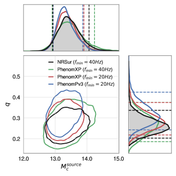
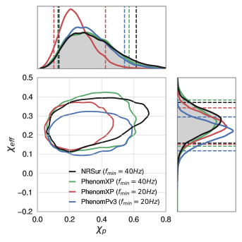
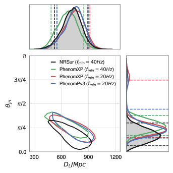
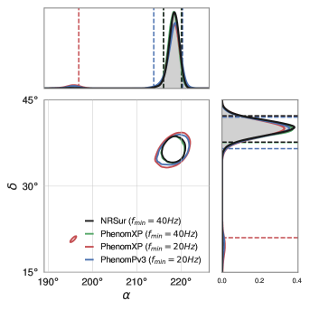
Figure 1: Estimated parameters for GW190412 using three different waveform models: NRSur7dq4, IMRPhenomXPHM and IMRPhenomPv3HM. While the NRSur7dq4 analysis is done with lower frequency cutoff $f_{\rm low}=40$ Hz, IMRPhenomXPHM parameter estimation has been carried out with two different values of minimum frequency: $f_{\rm low}=\{20,40\}$ Hz. In panel (a), we show the estimated two-dimensional contours for 90% confidence interval and one-dimensional kernel density estimates (KDEs) using Gaussian kernel for the source-frame chirp mass $\mathcal{M}^{\mathrm{source}}(M_{\odot}$) and mass ratio $q$. Panel (b), (c) and (d) report the corresponding contours and histograms for {effective inspiral spin $\chi_{\mathrm{eff}}$, spin precession $\chi_{p}$}, {luminosity distance $D_{L}$, orbital inclination angle $\theta_{JN}$} and {declination $\delta$, right ascension $\alpha$} respectively. Posteriors for NRSur7dq4 and IMRPhenomPv3HM are shown in black and blue receptively. For IMRPhenomXPHM, we plot the posteriors in red and green for analysis starting from 20 Hz and 40 Hz respectively. Dashed lines in the one-dimensional panels represent 90% credible intervals.

III Analyzing GW190412 Data

Since the NRSur7dq4 model is limited in waveform duration, we are forced to set a higher minimum frequency for the NRSur7dq4 analysis of GW190412 in this study as compared to Ref. Abbott et al. (2020a). We choose $f_{\rm low}=40$ Hz and a reference frequency $f_{\rm ref}=60$ Hz whenever analyzing the GW190412 data with NRSur7dq4. Furthermore, for the component masses of the binary, we use a narrower mass prior range as mentioned in Section II.3. We note that, for these choices of restricted mass priors, there are no signs of the posterior PDF railing against the prior bounds. The increased value of $f_{\rm low}$ in our analysis, as compared to the LVC analyses Abbott et al. (2020a), will necessarily incur some loss in the precision of the inferred parameters. In addition, we want make direct comparisons between the NRSur7dq4 results against analyses with other waveform approximants. To ensure a fair and direct approach for these comparisons, we deploy the following sequence of analysis:

• We first analyze the GW190412 data using IMRPhenomPv3HM with the same priors as used in LVC analysis and $f_{\rm low}=20$ Hz. We set $f_{\rm ref}$ to be 50 Hz. These results can then be used as a proxy for the LVC results also using the IMRPhenomPv3HM model Abbott et al. (2020a); LIGO Scientific Collaboration and Virgo Collaboration (2020b), but generated using our analysis procedure laid out in Section II. Note that we have used a setup to match the LVC one as best as possible with the parallel-bilby framework.

• We then repeat the analysis carried out in step 1, but using the new phenomenological waveform approximant IMRPhenomXPHM. Here, we are interested in if using a more modern phenomenological approximant creates any noticeable changes in the inferred parameter PDFs.

• Next, we perform a parameter estimation using IMRPhenomXPHM waveform model. However, we now change the setup to match the one we intend to use with NRSur7dq4. Namely, (i) the lower cutoff frequency and reference frequency are now set to $f_{\rm low}=40$ Hz and $f_{\rm ref}=60$ Hz respectively, (ii) the mass ratio is constrained to lie within $0.16\leq q\leq 1.00$, and (iii) a narrower component mass prior is used as mentioned in Sec. II.3.

• Finally, using the modified setup described in step 3, we redo the analysis with NRSur7dq4.

It is important to note that steps 1-3 are designed to investigate whether our results are affected by the choice of a higher value minimum frequency cut-off $f_{\rm low}$ and restricted prior range. Results from these four parameter estimations not only allow us to pinpoint any loss in accuracy and precision in inferring parameter properties due to a higher minimum frequency used for the NRSur7dq4 analysis, it enables direct comparison to the NRSur7dq4 results with the ones obtained using IMRPhenomXPHM within the same analysis setup.

III.1 Parameter Inference Results

In Table 2, we present the summary of the inferred source properties for GW190412 employing the NRSur7dq4 waveform approximant as well as phenom models (IMRPhenomPv3HM and IMRPhenomXPHM) with different minimum frequencies used in the Bayesian analysis. We report our results as median values and associated one-dimensional 90% credible intervals. We also compute the signal-to-noise Bayes factors Veitch and Vecchio (2010)

$$\mathcal{B}=\frac{\mathcal{Z_{\rm H}}}{\mathcal{Z_{\mathcal{N}}}},$$ (6)

where $\mathcal{Z_{\rm H}}$ and $\mathcal{Z_{\mathcal{N}}}$ denote the evidence for a signal model $H$ and a noise model $N$ respectively. The Bayes factor quantifies how much more likely that the data is described by a signal and not by random noise. We further report matched-filter signal-to-noise ratio (SNR) recovery (computed using pesummary Hoy and Raymond (2020); pes (2020)) for each of the waveform approximants. Posteriors of select parameters of interest are then shown in Fig. 1. Both the NRSur7dq4 and IMRPhenomXPHM models yield comparable values for their Bayes factors and SNRs when $f_{\rm low}$ is set to 40 Hz. Similarly, when $f_{\rm low}$ is set to 20 Hz, both IMRPhenomPv3HM and IMRPhenomXPHM recovers the signal with comparable Bayes factors and matched-filter SNR in all detectors. This suggests that any differences in the inferred parameters between models cannot be attributed to differences in the recovered SNR.

III.1.1 Mass Ratio

We first focus our attention to the mass recovery of different waveform models. We note that the most interesting parameters for GW190412 are its masses. A key result of our paper is the mass-ratio parameter recovery. We find that NRSur7dq4 favors a BBH signal with $q=0.26_{-0.08}^{+0.06}$, while the IMRPhenomPv3HM model recovers the signal with $0.31^{+0.11}_{-0.07}$. Therefore, the NRSur7dq4 estimate for the mass-ratio closely matches the value reported by the LVC obtained with the precessing EOB waveform model SEOBNRv4PHM Abbott et al. (2020a) but is in tension with the LVC’s IMRPhenomPv3HM result. Interestingly, IMRPhenomXPHM too favors $q\approx 1/4$. Taken together, our result strongly suggests that the progenitor of GW190412 is a $q=1/4$ BBH system and helps resolve the tension between mass-ratio estimates in LVC analysis with IMRPhenomPv3HM and SEOBNRv4PHM.

It is interesting to note that the mass-ratio inferred with the NRSur7dq4 model is better constrained compared to when obtained using the IMRPhenomXPHM model regardless of whether $f_{\rm low}$ was set to 20 Hz or 40 Hz (Fig.1). In fact, we do not observe any significant difference between the IMRPhenomXPHM mass-ratio posteriors inferred when using $f_{\rm low}=20$ Hz or $f_{\rm low}=40$ Hz. We attribute this improvement in the NRSur7dq4 result to not being dependent on the approximations that goes into currently available phenomenological modelling (including IMRPhenomXPHM).

We further note that the higher modes of IMRPhenomPv3HM are not calibrated to NR Khan et al. (2020). In addition, typical IMRPhenomPv3HM mismatch for GW190412 like binaries (i.e. $\sim 30-40$ $M_{\odot}$) is $\mathcal{M}\sim 1.5\times 10^{-2}$ Khan et al. (2020). This suggests inferred source properties for a GW190412-like binary using IMRPhenomPv3HM are likely to be biased if the newtork SNR is $\geq\sqrt{\frac{D}{2\mathcal{M}}}\sim 16.5$. This could explain the difference in mass-ratio estimates between IMRPhenomPv3HM and NRSur7dq4.

III.1.2 Chirp Mass

We find that the source-frame chirp mass $\mathcal{M}^{\mathrm{source}}$ posteriors for both IMRPhenomPv3HM ($13.22^{+0.52}_{-0.35}$) and IMRPhenomXPHM ($13.25^{+0.52}_{-0.29}$) using usual $f_{\rm low}=20$ Hz matches closely with each other (Fig.1). These estimates further match the reported LVC values Abbott et al. (2020a) obtained using IMRPhenomPv3HM and SEOBNRv4PHM models. On the other hand, NRSur7dq4 yields a broader posterior for $\mathcal{M}^{\mathrm{source}}$ ($13.27^{+0.60}_{-0.49}$). However, the $\mathcal{M}^{\mathrm{source}}$ posterior for NRSur7dq4 matches very closely with the IMRPhenomXPHM posterior ($13.35^{+0.73}_{-0.51}$) obtained using $f_{\rm low}=40$ Hz, the same value of minimum frequency cut-off set for NRSur7dq4 analysis. This indicates that the broadening in posterior for NRSur7dq4 can be attributed to the loss of information between 20 Hz and 40 Hz.

III.1.3 Spins

GW190412 is the first event with a strong constraint on $\chi_{1}$, the spin magnitude associated with the more massive BH. In Table 2 we report the inferred $\chi_{1}$ values using NRSur7dq4 ($0.48^{+0.26}_{-0.22}$), which mostly matches with the IMRPhenomXPHM analysis with $f_{\rm low}=40$ Hz ($0.47^{+0.21}_{-0.21}$). When setting the value of $f_{\rm low}$ to 20 Hz the IMRPhenomPv3HM model provides a slightly more constrained inference of $\chi_{1}$. Finally, we note that IMRPhenomXPHM provides a narrower estimation of the dimensionless primary spin magnitude $\chi_{1}$ ($0.39^{+0.16}_{-0.16}$) than IMRPhenomPv3HM ($0.40^{+0.21}_{-0.22}$) for an analysis that starts from 20Hz. The spin magnitude for the less massive BH remains uninformative for all models considered.

In Fig.1, we show the recovery of the effective inspiral spin parameter Ajith et al. (2011); Santamaria et al. (2010); Vitale et al. (2017),

$$\chi_{\mathrm{eff}}=\frac{m_{1}\chi_{1}\cos\theta_{1}+m_{2}\chi_{2}\cos\theta_{2}}{m_{1}+m_{2}}\,,$$ (7)

and the spin precession parameter Hannam et al. (2014b); Schmidt et al. (2015),

$$\chi_{p}=\max\left\{\chi_{1}\sin\theta_{1},\frac{q(4q+3)}{4+3q}\chi_{2}\sin\theta_{2}\right\}\,,$$ (8)

where $\theta_{1}$ and $\theta_{2}$ are the tilt angles between the spins and the orbital angular momentum respectively. We find that $\chi_{\mathrm{eff}}$ posteriors inferred with IMRPhenomPv3HM model are inconsistent with the ones inferred with NRSur7dq4 and IMRPhenomXPHM models. Moreover, the $\chi_{\mathrm{eff}}$ posteriors obtained using NRSur7dq4 and IMRPhenomXPHM models match with each other irrespective of whether $f_{\rm low}$ has been set to 20 Hz or 40 Hz for IMRPhenomXPHM

We use Jensen-Shannon (JS) divergence Lin (1991) to quantify the difference between the one-dimensional marginalized posteriors obtained with different waveform approximants. The JS divergence is a general symmetrized extension of the Kullback-Leibler divergence Kullback and Leibler (1951) with JS divergence values of 0.0 signifying that the posteriors are identical while a JS divergence value of 1.0 would mean the posterior distributions have no statistical overlap at all. We find that the JS divergence between $\chi_{\rm eff}$ posteriors obtained from IMRPhenomPv3HM and NRSur7dq4 is 0.336. Similarly, the JS divergence between $\chi_{\rm eff}$ posteriors obtained from IMRPhenomPv3HM and IMRPhenomXPHM is 0.304. For context, values above $0.15$ are sometimes considered to reflect non-negligible bias Abbott et al. (2019), and values near $0.4$ have large, noticeable bias. The $\chi_{\mathrm{eff}}$ posterior PDFs obtained using NRSur7dq4 and IMRPhenomXPHM models show better agreement with each other, somewhat irrespective of whether $f_{\rm low}$ has been set to 20 Hz or 40 Hz for IMRPhenomXPHM, producing a JS divergence of 0.13 and 0.07, respectively. The main difference between NRSur7dq4 and IMRPhenomXPHM ($f_{\rm low}=40$ Hz) $\chi_{\rm eff}$ posteriors is that the NRSur7dq4 one is slightly more constrained than IMRPhenomXPHM. This underscores the improvement in waveform modeling techniques in IMRPhenomXPHM over its predecessor IMRPhenomPv3HM.

As expected, when $f_{\rm low}$ is set to 40 Hz, the $\chi_{p}$ posterior for IMRPhenomXPHM becomes broader than the one inferred for the case with $f_{\rm low}=20$ Hz. The broadening of the posterior can be attributed to a reduction in the number of resolvable spin-precession cycles Hannam et al. (2014b); Schmidt et al. (2015); Pürrer et al. (2016); Fairhurst et al. (2020). While this is expected to be the dominant cause of broadening, care is required when comparing $\chi_{p}$ (and to a lesser extent $\chi_{\rm eff}$) posteriors recovered with different values of $f_{\rm ref}$ since both of these spin quantities are only approximately conserved throughout inspiral.

Interestingly, the $\chi_{p}$ posterior obtained using NRSur7dq4 provides more support for larger values of $\chi_{p}$. This is not entirely unexpected, as we do expect discrepancies between NRSur7dq4 and IMRPhenomXPHM to increase as the BBH system becomes more asymmetric Pratten et al. (2020). We return to this issue in Sec. III.3.

III.1.4 Inclination and luminosity distance

Another noteworthy aspect of our results in the recovery of luminosity distance and inclination angle between the line-of-sight and the direction of angular momentum of the BBH system (Fig.1). We find that the luminosity distance posterior recovered by NRSur7dq4 matches with both IMRPhenomPv3HM and IMRPhenomXPHM for the cases where $f_{\rm low}=20$ Hz. IMRPhenomXPHM yields smaller distances when $f_{\rm low}$ is set to $40$ Hz.

NRSur7dq4 also favors smaller values of inclination angle suggesting the system is closer to a face-on binary. This smaller value of inclination in NRSur7dq4 is potentially the reason for a broader $\chi_{p}$ posterior as precession is known to be less constrained for face-on binaries Chatziioannou et al. (2015); Vitale et al. (2014); O’Shaughnessy et al. (2014); Mandel et al. (2015); Littenberg et al. (2015). Such differences in the inferred luminosity distance and inclination between phenomenological model and NR surrogate models had also been observed while a phenomenological model IMRPhenomPv2 (the predecessor of IMRPhenomPv3HM) and an NR surrogate model NRSur7dq2 (predecessor of NRSur7dq4) were used for the analysis of GW150914 data Kumar et al. (2019). In that study, it was shown that the omission of subdominant modes in the IMRPhenomPv2 model was responsible for these differences. While the IMRPhenomXPHM model includes additional mode content $(\ell,m)=\{(2,\pm 1),(3,\pm 2),(3,\pm 3),(4,\pm 4)\}$, it is still missing many of the modes included in the NRSur7dq4 model, i.e. $(\ell,m)=\{(2,\pm 0),(3,\pm 0),(3,\pm 1),(4,\pm 0),(4,\pm 1),(4,\pm 2),(4,\pm 3)\}$. We suspect subdominant mode modeling may be responsible for the differences in the inferred luminosity distance and inclination seen here.

III.1.5 Source localization

In Fig. 1, we show the recovery of the sky location parameters. Both right ascension $\alpha$ and declination $\delta$ inferred using all three different waveform approximants, IMRPhenomPv3HM, IMRPhenomXPHM and NRSur7dq4, with both values of minimum frequencies ($f_{\rm low}=20$ Hz and $f_{\rm low}=40$ Hz) match well with each others. Using NRSur7dq4 model in analysis does not provide any extra information for the source’s location on the sky, when combined with the distance information shown in Fig. 1 the three dimensional volume does however change.

Table 2: Summary of the inferred parameters values for GW190412 (assuming the Planck 2015 cosmology Ade et al. (2016)). We report the median values with their 90% credible intervals, obtained using NRSur7dq4, a numerical relativity precessing surrogate model including higher multipoles. For comparison, we also show the results obtained using two different phenomenological models IMRPhenomPv3HM and IMRPhenomXPHM. For a direct comparison with the LVC results, we further show the reported parameter values for GW190412 (taken from Table II of Abbott et al. (2020a)). Parameter values inferred in this paper using IMRPhenomPv3HM and IMRPhenomXPHM here are broadly consistent with published LVC analyses.

	NRSur7dq4	PhenomPv3HM	PhenomXPHM	PhenomXPHM	PhenomPv3HM	SEOBNRv4HM
	($f_{\rm low}=40$ Hz)	($f_{\rm low}=20$ Hz)	($f_{\rm low}=20$ Hz)	($f_{\rm low}=40$ Hz)	(LVC Result Abbott et al. (2020a))	(LVC Result Abbott et al. (2020a))
$M/M_{\odot}$	$45.22^{+4.66}_{-3.80}$	$42.39^{+3.90}_{-3.44}$	$43.91^{+4.31}_{-3.51}$	$44.41^{+6.55}_{-4.08}$	$42.5^{+4.4}_{-3.7}$	$45.7^{+3.5}_{-3.3}$
$\mathcal{M}/M_{\odot}$	$15.26^{+0.70}_{-0.49}$	$15.22^{+0.28}_{-0.20}$	$15.26^{+0.36}_{-0.21}$	$15.16^{+0.79}_{-0.39}$	$15.2^{+0.3}_{-0.2}$	$15.3^{+0.1}_{-0.2}$
$m_{1}/M_{\odot}$	$35.85^{+5.51}_{-4.69}$	$32.25^{+4.99}_{-4.84}$	$34.20^{+5.36}_{-4.78}$	$34.88^{+7.99}_{-5.41}$	$32.3^{+5.7}_{-5.2}$	$36.5^{+4.2}_{-4.2}$
$m_{2}/M_{\odot}$	$9.34^{+1.33}_{-1.05}$	$10.12^{+1.52}_{-1.09}$	$9.7^{+1.34}_{-1.08}$	$9.46^{+1.70}_{-1.51}$	$10.1^{+1.6}_{-1.2}$	$9.2^{+0.9}_{-0.7}$
$M_{\mathrm{f}}/M_{\odot}$	$43.93^{+4.71}_{-3.86}$	$41.05^{+4.00}_{-3.54}$	$42.58^{+4.42}_{-3.62}$	$43.10^{+6.70}_{-4.17}$	-	-
$M^{\mathrm{source}}/M_{\odot}$	$39.50^{+3.84}_{-3.15}$	$36.86^{+3.21}_{-2.74}$	$38.15^{+3.67}_{-3.05}$	$39.10^{+5.48}_{-3.50}$	$36.9^{+3.7}_{-2.9}$	$39.7^{+3.0}_{-2.8}$
$\mathcal{M}^{\mathrm{source}}/M_{\odot}$	$13.27^{+0.60}_{-0.49}$	$13.22^{+0.52}_{-0.35}$	$13.25^{+0.52}_{-0.39}$	$13.35^{+0.73}_{-0.51}$	$13.3^{+0.5}_{-0.3}$	$13.3^{+0.3}_{-0.3}$
$m_{1}^{\mathrm{source}}/M_{\odot}$	$31.31^{+4.66}_{-3.97}$	$28.01^{+4.18}_{-3.98}$	$29.70^{+4.58}_{-4.07}$	$30.69^{+6.80}_{-4.62}$	$28.1^{+4.8}_{-4.3}$	$31.7^{+3.6}_{-3.5}$
$m_{2}^{\mathrm{source}}/M_{\odot}$	$8.15^{+1.19}_{-0.94}$	$8.78^{+1.47}_{-1.04}$	$8.42^{+1.25}_{-0.99}$	$8.32^{+1.58}_{-1.38}$	$8.8^{+1.6}_{-1.1}$	$8.0^{+0.9}_{-0.7}$
$M_{\mathrm{f}}^{\mathrm{source}}/M_{\odot}$	$38.36^{+3.92}_{-3.19}$	$35.66^{+3.29}_{-2.84}$	$37.00^{+3.74}_{-3.12}$	$37.94^{+5.60}_{-3.58}$	$35.7^{+3.8}_{-3.0}$	$38.6^{+3.1}_{-2.8}$
$q$	$0.26^{+0.08}_{-0.06}$	$0.31^{+0.11}_{-0.07}$	$0.28^{+0.09}_{-0.07}$	$0.27^{+0.10}_{-0.09}$	$0.31^{+0.12}_{-0.07}$	$0.25^{+0.06}_{-0.04}$
$\chi_{\mathrm{eff}}$	$0.27^{+0.10}_{-0.11}$	$0.22^{+0.08}_{-0.10}$	$0.25^{+0.09}_{-0.10}$	$0.26^{+0.12}_{-0.12}$	$0.22^{+0.08}_{-0.11}$	$0.28^{+0.06}_{-0.08}$
$\chi_{\mathrm{p}}$	$0.32^{+0.29}_{-0.19}$	$0.31^{+0.24}_{-0.17}$	$0.23^{+0.19}_{-0.13}$	$0.32^{+0.25}_{-0.19}$	$0.31^{+0.24}_{-0.17}$	$0.31^{+0.14}_{-0.15}$
$\chi_{1}$	$0.48^{+0.26}_{-0.22}$	$0.40^{+0.21}_{-0.22}$	$0.39^{+0.16}_{-0.16}$	$0.47^{+0.21}_{-0.21}$	$0.41^{+0.22}_{-0.24}$	$0.46^{+0.12}_{-0.15}$
$\chi_{2}$	$0.51^{+0.43}_{-0.45}$	$0.47^{+0.46}_{-0.42}$	$0.47^{+0.46}_{-0.42}$	$0.48^{+0.46}_{-0.43}$	$0.63^{+0.32}_{-0.52}$	$0.48^{+0.41}_{-0.41}$
$D_{\mathrm{L}}/\mathrm{Mpc}$	$720.54^{+165.39}_{-194.86}$	$749.59^{+149.09}_{-199.35}$	$749.68^{+166.21}_{-196.64}$	$671.76^{+176.53}_{-184.59}$	$740^{+150}_{-190}$	$740^{+120}_{-130}$
$\theta_{JN}$	$0.54^{+0.40}_{-0.34}$	$0.72^{+0.67}_{-0.28}$	$0.75^{+1.59}_{-0.29}$	$0.85^{+0.34}_{-0.32}$	$0.76^{+0.40}_{-0.29}$	$0.71^{+0.23}_{-0.21}$
$\rho_{\mathrm{H}}$	$9.15^{+0.21}_{-0.30}$	$9.35^{+0.19}_{-0.28}$	$9.23^{+0.17}_{-0.27}$	$9.11^{+0.19}_{-0.28}$	$9.5^{+0.2}_{-0.3}$	$9.5^{+0.1}_{-0.2}$
$\rho_{\mathrm{L}}$	$15.18^{+0.20}_{-0.30}$	$16.02^{+0.21}_{-0.28}$	$16.03^{+0.20}_{-0.27}$	$15.22^{+0.22}_{-0.28}$	$16.1^{+0.2}_{-0.3}$	$16.2^{+0.1}_{-0.2}$
$\rho_{\mathrm{V}}$	$4.02^{+0.26}_{-0.59}$	$3.53^{+0.35}_{-1.07}$	$3.58^{+0.27}_{-1.34}$	$4.03^{+0.25}_{-0.55}$	$3.6^{+0.3}_{-1.0}$	$3.7^{+0.2}_{-0.5}$
$\rho_{\mathrm{HLV}}$	$18.17^{+0.19}_{-0.30}$	$18.87^{+0.18}_{-0.28}$	$18.82^{+0.20}_{-0.31}$	$18.18^{+0.20}_{-0.30}$	$19.0^{+0.2}_{-0.3}$	$19.1^{+0.2}_{-0.2}$
$\ln\mathcal{B}_{\mathrm{s/n}}$	$131.99^{+0.24}_{-0.24}$	$144.49^{+0.21}_{-0.21}$	$143.38^{+0.24}_{-0.24}$	$131.92^{+0.23}_{-0.23}$	-	-

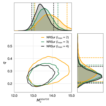
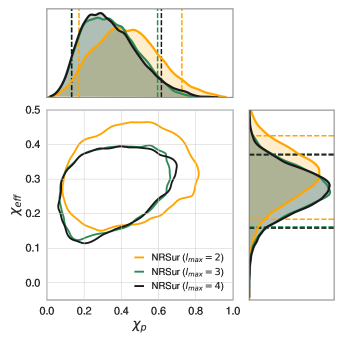
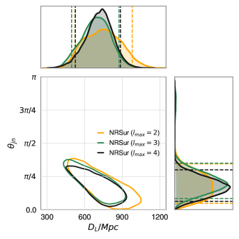
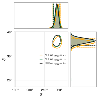
Figure 2: Estimated parameters for GW190412 using the NRSur7dq4 waveform model varying the spherical harmonic $(l,m)$ mode content . For all analyses, we use a lower frequency cutoff $f_{\rm low}=40$ Hz. In panel (a), we show the estimated two-dimensional contours for 90% confidence interval and one-dimensional KDEs using Gaussian kernel for the source-frame chirp mass $\mathcal{M}^{\mathrm{source}}(M_{\odot}$) and mass ratio $q$. Panel (b), (c) and (d) report the corresponding contours and histograms for {effective inspiral spin $\chi_{\mathrm{eff}}$, spin precession $\chi_{p}$}, {luminosity distance $D_{L}$, inclination angle $\theta_{JN}$} and {declination $\delta$, right ascension $\alpha$} respectively. Posteriors for NRSur7dq4 analysis with all modes $\ell_{max}=2$, $\ell_{max}=3$ and $\ell_{max}=4$ are plotted in orange, green and black lines respectively. Dashed lines in the one-dimensional posterior plots demarcate the 90% credible regions.

Table 3: Summary of the natural log Bayes factor and network matched filter signal-to-noise ratio (SNR) recovered using NRSur7dq4 model with different all $l\leq 2$ (i.e. $\ell_{\rm max}=2$), $\ell\leq 3$ (i.e. $\ell_{\rm max}=3$) and $\ell\leq 4$ (i.e. $\ell_{\rm max}=4$) modes respectively. The differences in log Bayes factor and SNR recovery demonstrates the importance of higher modes in GW data analysis.

	$\ln\mathcal{B}_{\mathrm{s/n}}$	$\rho_{\mathrm{HLV}}$
$\ell_{\rm max}=2$	$124.65^{+0.22}_{-0.22}$	$17.54^{+0.26}_{-0.36}$
$\ell_{\rm max}=3$	$131.62^{+0.24}_{-0.24}$	$18.09^{+0.20}_{-0.33}$
$\ell_{\rm max}=4$	$131.99^{+0.24}_{-0.24}$	$18.18^{+0.20}_{-0.30}$

III.2 Importance of subdominant modes

GW190412 is the first asymmetric mass ratio event detected by LIGO-Virgo collaboration and the first event for which significant SNR support has been observed for a mode other than the dominant quadrupolar mode. The LVC analysis finds considerable SNR in the $\ell=2,m=\pm 2$ (SNR $\sim 18.8$) and $\ell=3,m=\pm 3$ (SNR $\sim 3.3$) modes Abbott et al. (2020a); Mills and Fairhurst (2021). GW190412 therefore provides a prime testing ground to investigate the effects of higher modes in a GW data analysis on an astrophysical BBH observation.

In Fig. 2, we report the posterior PDFs obtained from analyzing the GW190412 data with the NRSur7dq4 model using different modes configurations: $\ell\leq 2$ (i.e. $\ell_{\rm max}=2$), $\ell\leq 3$ (i.e. $\ell_{\rm max}=3$) and $\ell\leq 4$ (i.e. $\ell_{\rm max}=4$) modes respectively including the $m=0$ memory modes.

In Table 3, we report the log Bayes factor and network matched filter signal-to-noise ratio (SNR) recovered using NRSur7dq4 model with different mode configurations. We find that even though the difference in SNR recovery between $\ell_{\rm max}=3$ and $\ell_{\rm max}=4$ analysis is small ($\sim 1$), including $\ell=4$ modes results in tighter constraints for the chirp mass (Fig.2), the luminosity distance (Fig.2), and the inclination angle (Fig.2). In some of the joint posteriors shown in Fig. 2 we also find that the posterior recovered with the $\ell_{\rm max}=2$ NRSur7dq4 model shows evidence for a secondary peak widely separated from the primary one. Similar spurious peaks were observed in mock parameter estimation studies with heavy BBH systems Shaik et al. (2020). The inference in the source localization parameters, namely, declination $\delta$ and right ascension $\alpha$ are not affected by the exclusion of $\ell=4$ modes (Fig.2).

Table 4: Summary of the JS divergence values between the one-dimensional marginalized posterior PDFs obtained using NRSur7dq4 with different mode configurations: $\ell_{\rm max}=2$, $\ell_{\rm max}=3$, and $\ell_{\rm max}=4$.

	JS-Divergnece	JS-Divergence
	between	between
	$\ell_{\rm max}=2$/$\ell_{\rm max}=4$	$\ell_{\rm max}=3$/$\ell_{\rm max}=4$
$\mathcal{M}^{\mathrm{source}}/M_{\odot}$	0.34	0.16
$q$	0.21	0.07
$\chi_{\mathrm{eff}}$	0.22	0.02
$\chi_{\mathrm{p}}$	0.19	0.03
$D_{\mathrm{L}}/\mathrm{Mpc}$	0.18	0.08
$\theta_{JN}$	0.13	0.12
$\alpha$	0.21	0.11
$\delta$	0.24	0.04

To quantify the difference between key posteriors obtained using different mode configurations, we compute the JS divergence Lin (1991) between the one-dimensional marginalized posterior. In Table 4, we summarize the JS divergence values for between select posterior obtained using different values of $\ell_{\rm max}$. It is evident that not using any higher harmonics beyond $\ell=2$ results in significantly different posteriors for almost all intrinsic and extrinsic parameters. Omitting only $\ell=4$ modes, however, has only marginal effects on the posterior of most parameters, except for the source frame chirp mass and inclination angle. As an $\ell=5$ surrogate model is currently unavailable, we are unable to test whether this family of harmonic mode content would be needed to ensure a sufficiently converged posterior in these two parameters.

III.3 Effect of modelling approximations

We now attempt to explain the differences between NRSur7dq4 and IMRPhenomXPHM posteriors (cf. the $\chi_{\mathrm{eff}}-\chi_{p}$ posterior in Fig. 1) by imposing two IMRPhenomXPHM modeling assumptions (also discussed in Bruegmann et al. (2008); Ramos-Buades et al. (2020)) into the surrogate.

The first modeling assumption made by IMRPhenomXPHM (and many other models) is that the binary black hole system has orbital plane symmetry in the co-precessing frame. This is to say that the asymmetric modes are zero. These modes measure the extent to which the non-precessing formula, $h_{\ell,-m}=(-1)^{\ell} h_{\ell,m}^{*}$, relating positive and negative $m$ modes is violated in the co-precessing frame. While mode asymmetries of the waveform from precessing systems is a small effect, these features cannot be completely removed with a different choice of frame Boyle et al. (2014) and are generally non-zero even in a co-precessing frame. In the surrogate model, this approximation can be implemented by setting the asymmetric modes to zero (blue line; Fig.3).

The second modeling assumption made by the phenomological family of models is that in the co-precessing frame the waveform modes are described by an aligned-spin BBH system . In the surrogate model, this approximation can be implemented by setting the in-plane spins in the co-precessing frame to zero (green line; Fig.3). Note that this second modeling assumption clearly implies the first.

Neither of these approximations has any appreciable difference on the posteriors, which suggests that other modeling approximations are responsible for the deviations observed in Fig. 1.

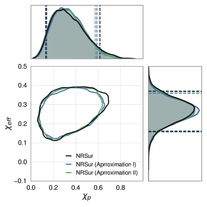
Figure 3: Estimated effective inspiral spin$\chi_{\mathrm{eff}}$ and spin precession $\chi_{p}$ for GW190412 event using NRSur7dq4 waveform. We show the two-dimensional contours and one-dimensional KDEs using Gaussian kernel of $\chi_{\mathrm{eff}}$ and $\chi_{p}$ obtained using the NRSur7dq4 waveform model in black. We then show the posteriors using NRSur7dq4 after imposing two different modelling approximations that are often assumed for building phenomenological and EOB models. The posteriors recovered (i) after the omission of asymmetric modes is shown in light blue (“Approximation I") and (i) assuming the model reduces to an aligned-spin model in the co-precessing frame is shown in deep blue (“Approximation II"). [Details in text; See Section III.3]. We find no noticeable difference between posteriors obtained from default NRSur7dq4 model and these approximations.

IV Discussion and Conclusion

In this paper, we used the numerical relativity-based precessing surrogate model, NRSur7dq4, to analyze the BBH signal GW190412 employing a fully Bayesian framework. Restrictive waveform durations in the NRSur7dq4 model has forced us to set the lower frequency cutoff to be 40 Hz instead of the usual 20 Hz. Despite this limitation, we demonstrate that an analysis using the NRSur7dq4 model is able to efficiently infer binary properties from the observed GW signal.

Our analysis broadly agrees with the published LVC results using SEOBNRv4PHM and is in disagreement with the LVC results using IMRPhenomPv3HM. As such, we believe our results can serve to help resolve the tension between mass-ratio and spin estimates in the official LVC analysis.

We also find that NRSur7dq4 provides improved constraints for the mass-ratio, spin precession, luminosity distance and inclination. Using the NRSur7dq4 model we have been able to provide a better constraint on the mass ratio than the state-of-art phenomenological waveform model IMRPhenomXPHM. Furthermore, we show the binary to be more close to a face-on system which results in less constrained estimation of the spin precession parameter. All these result, taken together, indicate that numerical-relativity based surrogate models could help to extract more information of BBH mergers from events like GW190412. This is because surrogates have been extensively trained on numerical simulations of precessing systems and include all of the most important subdominant modes. We also recommend that future numerical-relativity surrogates should include $\ell_{\rm max}>4$ harmonic modes as these could be important for the inference of certain parameters (cf. Sec. III.2).

Another direction of the paper has been to investigate the effects of subdominant modes in parameter estimation with real data instead of synthetic GW datasets. Using the NRSur7dq4 model we perform parameter inference using a sequence of $\ell_{\rm max}=2,3,$ and $4$ harmonics modes, where $\ell_{\rm max}=4$ corresponds to all modes available in NRSur7dq4. We find that, even though the increase in recovered SNR using $\ell=4$ modes is negligible, the omission of subdominant modes can affect the posteriors quite significantly. When using only $\ell_{\rm max}=2$ modes we find that all parameters are biased (cf. Table 4) and some posteriors develop spurious secondary peaks. When including $\ell_{\rm max}=3$ modes the chirp mass and inclination angles still show moderate bias. While we suspect $\ell_{\rm max}=4$ modes should be sufficient to resolve the posterior, currently no model has a complete family of $\ell_{\rm max}=5$ modes to check this. As more binaries with asymmetric masses are detected, the modelling of higher order modes will become increasingly important even if the SNR contribution from each individual mode is small.

This study also presents a new opportunity to explore how modelling can affect posteriors – sometimes non-trivially. We note that even though both NRSur7dq4 and IMRPhenomXPHM model have higher modes and spin precession, results obtained using these two models do not always agree. Specially, the estimates of mass ratio, spin precession, luminosity distance, and inclination differs depending on which of these two models have been used to analyze the data. The difference in modelling higher order modes and spin effects could potentially be the reason for the observed difference in parameter estimation. We attempted to explain our observed differences by considering two approximations widely used in many effective one body and phenomenological waveform families to model the spin effects: (i) a binary system has orbital plane symmetry in co-precessing frame; and (ii) the gravitational-wave modes in the binary’s co-precessing frame is described by an aligned-spin system. We find that, for low SNR event like GW190412, such assumptions do not change the posteriors in any significant way. However, with events having higher SNRs, these approximations might yield differences in the recovered posteriors.

Appendix A Parameter Estimation with Synthetic GW Signals

Since the NRSur7dq4 model has not been extensively used in many parameter estimation studies so far, except for analyzing the GW150914 event Varma et al. (2020) and the recent GW190521 high-mass BBH Abbott et al. (2020c), we perform an injection study to understand potential systematics in greater detail. We generate synthetic GW signals with NRSur7dq4 model using all available $l\leq 4$ modes and inject them in the three-detector LVC network consisting of the LIGO-Hanford, LIGO-Livingston, and Virgo detectors. We then estimate the signal properties using the Bayesian framework described in Section II. We assume design sensitivity for each of the LIGO-Virgo detectors and use a zero noise configuration.

We choose the injected BBH parameters such that they match the GW190412 properties as inferred from the LVC analysis Abbott et al. (2020a). We note that the inferred values for the mass-ratio in LVC analysis with IMRPhenomPv3HM and SEOBNRv4HM do not match with each other. While PE with IMRPhenomPv3HM model indicates a mass ratio of $q=0.33_{-0.09}^{+0.12}$, SEOBNRv4HM prefers a more asymmetric mass ratio $q=0.25_{-0.04}^{+0.06}$. We therefore simulate two different synthetic GW signals – with mass-ratio $q_{\rm inj}=0.25$ and $q_{\rm inj}=0.33$, respectively. This ensures that our injection study is relevant for asymmetric mass-ratio events like GW190412. All other parameter values for both the injections are same. Both the signals were created at a luminosity distance of $D_{L}=730$ Mpc and with inclination angle $\theta_{JN}=0.73$. We choose dimensionless spin parameters $\chi_{1}=0.43$ and $\chi_{2}=0.55$; and spin angles as: $\theta_{1}=1.05$ and $\theta_{2}=1.01$, $\phi_{12}=3.53$ and $\phi_{jl}=3.75$ respectively (cf. Appendix of Romero-Shaw et al. (2020) for definitions of these parameters). This corresponds to an effective inspiral spin of $\chi_{\mathrm{eff}}=0.3$ and spin precession of $\chi_{p}=0.4$. The chosen sky localization for the injected signals is: right ascension $\alpha=218.29\degree$ and declination $\delta=36.09\degree$. We set $f_{\rm low}=40$ Hz and $f_{\rm ref}=60$ Hz.

We find that NRSur7dq4 model successfully recovers the injected source properties. In Fig.4, we show the recovered posteriors for both the injections. Posteriors for $q_{\rm inj}=0.25$ is shown in violet whereas $q_{\rm inj}=0.33$ posteriors are plotted in orange. We find that while both chirp mass and effective spin of the BBH are estimated with comparable precision for both the injections, the mass-ratio and spin precession is well constrained for more asymmetric signal (i.e for $q_{\rm inj}=0.25$). For the extrinsic parameters, we find no significant difference in the recovered posteriors. This injection study demonstrates the efficacy of NRSur7dq4 waveform model to successfully recover a true signal from strain data.

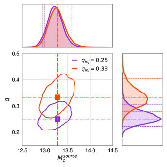
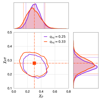
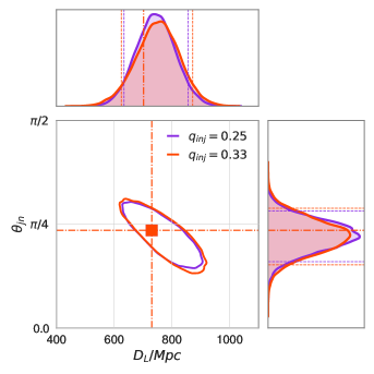
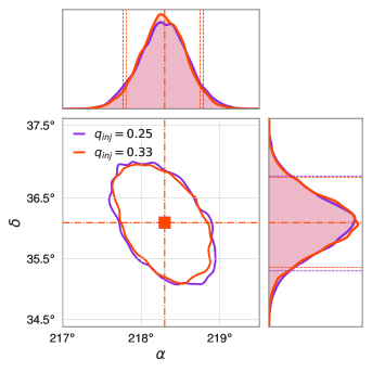
Figure 4: Parameter recovery for the synthetic injections with the NRSur7dq4 waveform model for two different values of mass ratio: $q_{inj}=0.33$ and $q_{inj}=0.25$. In (a), we show the estimated two-dimensional contours for 90% confidence interval and one-dimensional KDEs for the source-frame chirp mass $\mathcal{M}^{\mathrm{source}}(M_{\odot}$) and mass ratio $q$. Panel (b), (c) and (d) report the corresponding contours and KDEs using Gaussian kernel for {effective inspiral spin $\chi_{\mathrm{eff}}$, spin precession $\chi_{p}$}, {luminosity distance $D_{L}$, inclination angle $\theta_{JN}$} and {declination $\delta$, right ascension $\alpha$} respectively. Posteriors for $q_{inj}=0.25$ are shown in violet while $q_{inj}=0.33$ posteriors are plotted in orange. In both two-dimensional and one-dimensional panels, dashed dotted lines indicate the true injection values. Dashed lines in the one-dimensional panels represent 90% credible regions.

References

References

- Harry (2010) G. M. Harry (LIGO Scientific Collaboration), Class. Quant. Grav. 27, 084006 (2010).
- Acernese et al. (2015) F. Acernese et al. (Virgo Collaboration), Class. Quant. Grav. 32, 024001 (2015), arXiv:1408.3978 [gr-qc] .
- Abbott et al. (2020a) R. Abbott et al. (LIGO Scientific, Virgo), Phys. Rev. D 102, 043015 (2020a), arXiv:2004.08342 [astro-ph.HE] .
- LIGO Scientific Collaboration and Virgo Collaboration (2020a) LIGO Scientific Collaboration and Virgo Collaboration, “The GW190412 Data Release,” (2020a).
- Bohé et al. (2017) A. Bohé et al., Phys. Rev. D 95, 044028 (2017), arXiv:1611.03703 [gr-qc] .
- Cotesta et al. (2018) R. Cotesta, A. Buonanno, A. Bohé, A. Taracchini, I. Hinder, and S. Ossokine, Phys. Rev. D 98, 084028 (2018), arXiv:1803.10701 [gr-qc] .
- Cotesta et al. (2020) R. Cotesta, S. Marsat, and M. Pürrer, Phys. Rev. D 101, 124040 (2020), arXiv:2003.12079 [gr-qc] .
- Pan et al. (2014) Y. Pan, A. Buonanno, A. Taracchini, L. E. Kidder, A. H. Mroué, H. P. Pfeiffer, M. A. Scheel, and B. Szilágyi, Phys. Rev. D 89, 084006 (2014), arXiv:1307.6232 [gr-qc] .
- Babak et al. (2017) S. Babak, A. Taracchini, and A. Buonanno, Phys. Rev. D 95, 024010 (2017), arXiv:1607.05661 [gr-qc] .
- Husa et al. (2016) S. Husa, S. Khan, M. Hannam, M. Pürrer, F. Ohme, X. Jiménez Forteza, and A. Bohé, Phys. Rev. D 93, 044006 (2016), arXiv:1508.07250 [gr-qc] .
- Khan et al. (2016) S. Khan, S. Husa, M. Hannam, F. Ohme, M. Pürrer, X. Jiménez Forteza, and A. Bohé, Phys. Rev. D 93, 044007 (2016), arXiv:1508.07253 [gr-qc] .
- London et al. (2018) L. London, S. Khan, E. Fauchon-Jones, C. García, M. Hannam, S. Husa, X. Jiménez-Forteza, C. Kalaghatgi, F. Ohme, and F. Pannarale, Phys. Rev. Lett. 120, 161102 (2018), arXiv:1708.00404 [gr-qc] .
- Khan et al. (2019) S. Khan, K. Chatziioannou, M. Hannam, and F. Ohme, Phys. Rev. D 100, 024059 (2019), arXiv:1809.10113 [gr-qc] .
- Hannam et al. (2014a) M. Hannam, P. Schmidt, A. Bohé, L. Haegel, S. Husa, F. Ohme, G. Pratten, and M. Pürrer, Phys. Rev. Lett. 113, 151101 (2014a), arXiv:1308.3271 [gr-qc] .
- Khan et al. (2020) S. Khan, F. Ohme, K. Chatziioannou, and M. Hannam, Phys. Rev. D 101, 024056 (2020), arXiv:1911.06050 [gr-qc] .
- Varma et al. (2019a) V. Varma, S. E. Field, M. A. Scheel, J. Blackman, L. E. Kidder, and H. P. Pfeiffer, Phys. Rev. D 99, 064045 (2019a), arXiv:1812.07865 [gr-qc] .
- Varma and Ajith (2017) V. Varma and P. Ajith, Phys. Rev. D96, 124024 (2017), arXiv:1612.05608 [gr-qc] .
- Calderón Bustillo et al. (2016) J. Calderón Bustillo, S. Husa, A. M. Sintes, and M. Pürrer, Phys. Rev. D93, 084019 (2016), arXiv:1511.02060 [gr-qc] .
- Capano et al. (2014) C. Capano, Y. Pan, and A. Buonanno, Phys. Rev. D89, 102003 (2014), arXiv:1311.1286 [gr-qc] .
- Littenberg et al. (2013) T. B. Littenberg, J. G. Baker, A. Buonanno, and B. J. Kelly, Phys. Rev. D 87, 104003 (2013), arXiv:1210.0893 [gr-qc] .
- Calderón Bustillo et al. (2017) J. Calderón Bustillo, P. Laguna, and D. Shoemaker, Phys. Rev. D95, 104038 (2017), arXiv:1612.02340 [gr-qc] .
- Brown et al. (2013) D. A. Brown, P. Kumar, and A. H. Nitz, Phys. Rev. D 87, 082004 (2013), arXiv:1211.6184 [gr-qc] .
- Varma et al. (2014) V. Varma, P. Ajith, S. Husa, J. C. Bustillo, M. Hannam, and M. Pürrer, Phys. Rev. D 90, 124004 (2014), arXiv:1409.2349 [gr-qc] .
- Graff et al. (2015) P. B. Graff, A. Buonanno, and B. S. Sathyaprakash, Phys. Rev. D 92, 022002 (2015), arXiv:1504.04766 [gr-qc] .
- Harry et al. (2018) I. Harry, J. Calderón Bustillo, and A. Nitz, Phys. Rev. D97, 023004 (2018), arXiv:1709.09181 [gr-qc] .
- Chatziioannou et al. (2019a) K. Chatziioannou et al., Phys. Rev. D 100, 104015 (2019a), arXiv:1903.06742 [gr-qc] .
- Shaik et al. (2020) F. H. Shaik, J. Lange, S. E. Field, R. O’Shaughnessy, V. Varma, L. E. Kidder, H. P. Pfeiffer, and D. Wysocki, Phys. Rev. D 101, 124054 (2020), arXiv:1911.02693 [gr-qc] .
- Kumar et al. (2019) P. Kumar, J. Blackman, S. E. Field, M. Scheel, C. R. Galley, M. Boyle, L. E. Kidder, H. P. Pfeiffer, B. Szilagyi, and S. A. Teukolsky, Phys. Rev. D 99, 124005 (2019), arXiv:1808.08004 [gr-qc] .
- Abbott et al. (2016a) B. Abbott et al. (LIGO Scientific, Virgo), Phys. Rev. Lett. 116, 061102 (2016a), arXiv:1602.03837 [gr-qc] .
- Abbott et al. (2017) B. P. Abbott et al. (LIGO Scientific, VIRGO), Phys. Rev. Lett. 118, 221101 (2017), [Erratum: Phys.Rev.Lett. 121, 129901 (2018)], arXiv:1706.01812 [gr-qc] .
- Blackman et al. (2017a) J. Blackman, S. E. Field, M. A. Scheel, C. R. Galley, C. D. Ott, M. Boyle, L. E. Kidder, H. P. Pfeiffer, and B. Szilágyi, Phys. Rev. D 96, 024058 (2017a), arXiv:1705.07089 [gr-qc] .
- Varma et al. (2019b) V. Varma, S. E. Field, M. A. Scheel, J. Blackman, D. Gerosa, L. C. Stein, L. E. Kidder, and H. P. Pfeiffer, Phys. Rev. Research. 1, 033015 (2019b), arXiv:1905.09300 [gr-qc] .
- Pratten et al. (2020) G. Pratten et al., ArXiv e-prints (2020), arXiv:2004.06503 [gr-qc] .
- Farr et al. (2015) W. M. Farr, B. Farr, and T. Littenberg, Modelling Calibration Errors In CBC Waveforms, Tech. Rep. LIGO-T1400682 (LIGO Project, 2015).
- Romero-Shaw et al. (2020) I. M. Romero-Shaw et al., Mon. Not. Roy. Astron. Soc. 499, 3295 (2020), arXiv:2006.00714 [astro-ph.IM] .
- LIGO Scientific Collaboration and Virgo Collaboration (2020b) LIGO Scientific Collaboration and Virgo Collaboration, “Parameter estimation sample release for GW190412,” (2020b).
- Ashton et al. (2019) G. Ashton et al., Astrophys. J. Suppl. 241, 27 (2019), arXiv:1811.02042 [astro-ph.IM] .
- Smith et al. (2020) R. J. E. Smith, G. Ashton, A. Vajpeyi, and C. Talbot, Mon. Not. Roy. Astron. Soc. 498, 4492 (2020), arXiv:1909.11873 [gr-qc] .
- Speagle (2020) J. S. Speagle, Mon. Not. Roy. Astron. Soc. 493, 3132 (2020), arXiv:1904.02180 [astro-ph.IM] .
- pe_(2021) “GW190412 parameter estimation data, posteriors, and input files accompanying this paper,” (2021).
- Abbott et al. (2021) R. Abbott et al. (LIGO Scientific, Virgo), SoftwareX 13, 100658 (2021), arXiv:1912.11716 [gr-qc] .
- Littenberg and Cornish (2015) T. B. Littenberg and N. J. Cornish, Phys. Rev. D 91, 084034 (2015), arXiv:1410.3852 [gr-qc] .
- Cornish and Littenberg (2015) N. J. Cornish and T. B. Littenberg, Class. Quant. Grav. 32, 135012 (2015), arXiv:1410.3835 [gr-qc] .
- Chatziioannou et al. (2019b) K. Chatziioannou, C.-J. Haster, T. B. Littenberg, W. M. Farr, S. Ghonge, M. Millhouse, J. A. Clark, and N. Cornish, Phys. Rev. D 100, 104004 (2019b), arXiv:1907.06540 [gr-qc] .
- gws (2020) “GWSurrogate,” https://github.com/sxs-collaboration/gwsurrogate/ (2020).
- Field et al. (2014) S. E. Field, C. R. Galley, J. S. Hesthaven, J. Kaye, and M. Tiglio, Phys. Rev. X 4, 031006 (2014), arXiv:1308.3565 [gr-qc] .
- LIGO Scientific Collaboration (2020) LIGO Scientific Collaboration, “LIGO Algorithm Library - LALSuite,” free software (GPL) (2020).
- Field et al. (2011) S. E. Field, C. R. Galley, F. Herrmann, J. S. Hesthaven, E. Ochsner, and M. Tiglio, Phys. Rev. Lett. 106, 221102 (2011), arXiv:1101.3765 [gr-qc] .
- Blackman et al. (2017b) J. Blackman, S. E. Field, M. A. Scheel, C. R. Galley, D. A. Hemberger, P. Schmidt, and R. Smith, Phys. Rev. D95, 104023 (2017b), arXiv:1701.00550 [gr-qc] .
- Abbott et al. (2020b) R. Abbott et al. (LIGO Scientific, Virgo), Phys. Rev. Lett. 125, 101102 (2020b), arXiv:2009.01075 [gr-qc] .
- Abbott et al. (2020c) R. Abbott et al. (LIGO Scientific, Virgo), Astrophys. J. Lett. 900, L13 (2020c), arXiv:2009.01190 [astro-ph.HE] .
- Flanagan and Hughes (1998) E. E. Flanagan and S. A. Hughes, Phys. Rev. D 57, 4535 (1998), arXiv:gr-qc/9701039 .
- Lindblom et al. (2008) L. Lindblom, B. J. Owen, and D. A. Brown, Phys. Rev. D 78, 124020 (2008), arXiv:0809.3844 [gr-qc] .
- McWilliams et al. (2010) S. T. McWilliams, B. J. Kelly, and J. G. Baker, Phys. Rev. D 82, 024014 (2010), arXiv:1004.0961 [gr-qc] .
- Pürrer and Haster (2020) M. Pürrer and C.-J. Haster, Phys. Rev. Res. 2, 023151 (2020), arXiv:1912.10055 [gr-qc] .
- Chatziioannou et al. (2017) K. Chatziioannou, A. Klein, N. Cornish, and N. Yunes, Phys. Rev. Lett. 118, 051101 (2017), arXiv:1606.03117 [gr-qc] .
- Abbott et al. (2016b) B. Abbott et al. (LIGO Scientific, Virgo), Phys. Rev. D 94, 064035 (2016b), arXiv:1606.01262 [gr-qc] .
- Harris (1978) F. J. Harris, Proceedings of the IEEE 66, 51 (1978).
- Abbott et al. (2020d) R. Abbott et al. (LIGO Scientific, Virgo), Astrophys. J. Lett. 896, L44 (2020d), arXiv:2006.12611 [astro-ph.HE] .
- Zevin et al. (2020) M. Zevin, C. P. Berry, S. Coughlin, K. Chatziioannou, and S. Vitale, Astrophys. J. Lett. 899, L17 (2020), arXiv:2006.11293 [astro-ph.HE] .
- Veitch and Vecchio (2010) J. Veitch and A. Vecchio, Phys. Rev. D 81, 062003 (2010), arXiv:0911.3820 [astro-ph.CO] .
- Hoy and Raymond (2020) C. Hoy and V. Raymond, (2020), arXiv:2006.06639 [astro-ph.IM] .
- pes (2020) “pesummary,” https://github.com/pesummary/pesummary/tree/v0.6.0 (2020).
- Ajith et al. (2011) P. Ajith et al., Phys. Rev. Lett. 106, 241101 (2011), arXiv:0909.2867 [gr-qc] .
- Santamaria et al. (2010) L. Santamaria et al., Phys. Rev. D 82, 064016 (2010), arXiv:1005.3306 [gr-qc] .
- Vitale et al. (2017) S. Vitale, R. Lynch, V. Raymond, R. Sturani, J. Veitch, and P. Graff, Phys. Rev. D 95, 064053 (2017), arXiv:1611.01122 [gr-qc] .
- Hannam et al. (2014b) M. Hannam, P. Schmidt, A. Bohé, L. Haegel, S. Husa, F. Ohme, G. Pratten, and M. Pürrer, Phys. Rev. Lett. 113, 151101 (2014b), arXiv:1308.3271 [gr-qc] .
- Schmidt et al. (2015) P. Schmidt, F. Ohme, and M. Hannam, Phys. Rev. D 91, 024043 (2015), arXiv:1408.1810 [gr-qc] .
- Lin (1991) J. Lin, IEEE Transactions on Information Theory 37, 145 (1991).
- Kullback and Leibler (1951) S. Kullback and R. A. Leibler, Ann. Math. Statist. 22, 79 (1951).
- Abbott et al. (2019) B. P. Abbott et al. (LIGO Scientific, Virgo), Phys. Rev. X9, 031040 (2019), arXiv:1811.12907 [astro-ph.HE] .
- Pürrer et al. (2016) M. Pürrer, M. Hannam, and F. Ohme, Phys. Rev. D 93, 084042 (2016), arXiv:1512.04955 [gr-qc] .
- Fairhurst et al. (2020) S. Fairhurst, R. Green, C. Hoy, M. Hannam, and A. Muir, Phys. Rev. D 102, 024055 (2020), arXiv:1908.05707 [gr-qc] .
- Chatziioannou et al. (2015) K. Chatziioannou, N. Cornish, A. Klein, and N. Yunes, Astrophys. J. Lett. 798, L17 (2015), arXiv:1402.3581 [gr-qc] .
- Vitale et al. (2014) S. Vitale, R. Lynch, J. Veitch, V. Raymond, and R. Sturani, Phys. Rev. Lett. 112, 251101 (2014), arXiv:1403.0129 [gr-qc] .
- O’Shaughnessy et al. (2014) R. O’Shaughnessy, B. Farr, E. Ochsner, H.-S. Cho, V. Raymond, C. Kim, and C.-H. Lee, Phys. Rev. D 89, 102005 (2014), arXiv:1403.0544 [gr-qc] .
- Mandel et al. (2015) I. Mandel, C.-J. Haster, M. Dominik, and K. Belczynski, Mon. Not. Roy. Astron. Soc. 450, L85 (2015), arXiv:1503.03172 [astro-ph.HE] .
- Littenberg et al. (2015) T. B. Littenberg, B. Farr, S. Coughlin, V. Kalogera, and D. E. Holz, Astrophys. J. Lett. 807, L24 (2015), arXiv:1503.03179 [astro-ph.HE] .
- Ade et al. (2016) P. Ade et al. (Planck), Astron. Astrophys. 594, A13 (2016), arXiv:1502.01589 [astro-ph.CO] .
- Mills and Fairhurst (2021) C. Mills and S. Fairhurst, Phys. Rev. D 103, 024042 (2021), arXiv:2007.04313 [gr-qc] .
- Bruegmann et al. (2008) B. Bruegmann, J. A. Gonzalez, M. Hannam, S. Husa, and U. Sperhake, Phys. Rev. D 77, 124047 (2008), arXiv:0707.0135 [gr-qc] .
- Ramos-Buades et al. (2020) A. Ramos-Buades, P. Schmidt, G. Pratten, and S. Husa, Phys. Rev. D 101, 103014 (2020), arXiv:2001.10936 [gr-qc] .
- Boyle et al. (2014) M. Boyle, L. E. Kidder, S. Ossokine, and H. P. Pfeiffer, ArXiv e-prints (2014), arXiv:1409.4431 [gr-qc] .
- Varma et al. (2020) V. Varma, M. Isi, and S. Biscoveanu, Phys. Rev. Lett. 124, 101104 (2020), arXiv:2002.00296 [gr-qc] .