Paying down metadata debt: learning the representation of concepts using topic models

Abstract.

We introduce a data management problem called metadata debt, to identify the mapping between data concepts and their logical representations. We describe how this mapping can be learned using semisupervised topic models based on low-rank matrix factorizations that account for missing and noisy labels, coupled with sparsity penalties to improve localization and interpretability. We introduce a gauge transformation approach that allows us to construct explicit associations between topics and concept labels, and thus assign meaning to topics. We also show how to use this topic model for semisupervised learning tasks like extrapolating from known labels, evaluating possible errors in existing labels, and predicting missing features. We show results from this topic model in predicting subject tags on over 25,000 datasets from Kaggle.com, demonstrating the ability to learn semantically meaningful features.

1. Introduction

“What data do I have?” is a surprisingly difficult question to answer when managing data at the scale of large organizations (Khatri and Brown, 2010). A complete answer requires not just the physical location of data (what database or filesystem?), but also the corresponding logical representation (what attributes and relations?) and conceptual formulation (what business semantics?) (West, 2003). Understanding the relationship between these successive levels of abstraction is necessary in order to define data governance needs such as data quality rules (Wang and Strong, 1996).

As a simple example, suppose we need to enforce a rule that the balance on the customer’s account is positive. To define a data quality check, we need to know to look up the table ACCOUNTS, find the row that matches the current account ID in the column ACCT_ID, and check that the corresponding entry in the ACCT_BAL column is not missing and is a positive number. Translating the conceptual business need into a computable statement thus requires explicit knowledge of the semantic concepts in the data (“account” and “balance”) and the logical representation of that data (which tables and columns). Having a complete inventory of concepts and their logical representations is therefore a key component of data governance, even being a regulatory requirement for compliance with Basel standards (Basel Committee on Banking Supervision, 2013) and others.

In practice, however, organizations often lack the metadata needed to describe the conceptual–logical mapping we have just described. For example, collaborative tagging from crowdsourced data quickly yields folksonomies of conceptual tags, but they may be inconsistent due to personal biases and therefore require standardization (Guy and Tonkin, 2006). Other situations arise in legacy enterprises, where the merger of multiple information systems results in multiple logical representations of the same data concept, or when loss of informal knowledge or incomplete documentation results in an incompletely documented system, or when a legacy system is repurposed for a new business purpose, whose conceptual needs are not perfectly aligned with the existing logical layout of data. Furthermore, the cost of correctly assigning concept labels can be very high when the semantic definition of the concepts is couched in technical jargon which requires subject matter expertise to comprehend. Similarly, similar concepts may require expertise to disambiguate and label correctly. The challenge of correct conceptual labeling is exacerbated when the controlled vocabulary evolves over time, a phenomenon known as concept drift (Wang et al., 2011),or when the logical representation of data also changes, as APIs and data formats change (Gama et al., 2014). Therefore, it is possible that despite the best intentions and efforts of organizations, that they still struggle to maintain and verify that they have a correct and up-to-date conceptual–logical mapping of data.

In this paper, we study the problem of metadata debt, namely the technical debt incurred when an organization lacks a complete and current mapping between its data concepts and their corresponding logical representations. We propose in Section 2 to use semisupervised topic modeling to learn the conceptual–logical mapping of data, making full use of existing concept labels, be they incomplete or noisy. We first describe how an unsupervised topic model like latent semantic indexing (LSI) contains a hidden invariance that we can exploit to write down an unambiguous, gauge-generalized variant (GG-LSI) for the semisupervised setting in Sections 2.2 and 2.3. Next, we show how a more sophisticated semisupervised topic model can be expressed in the formalism of generalized low-rank models (GLRMs) in Section 2.4, which allows us to specify a combination of elementwise logistic losses with customizable sparsity penalties. We illustrate with a simple example how to interpret the results of all these methods in Sections 2.1 and 2.5. Next, we describe in Section 3 how to use the numerical trick of randomized subsampling to greatly reduce the computational cost of topic modeling, and GLRMs in particular, so that the compute time is asymptotically linear in the number of topics. This linear-time trick allows us to compute GLRMs efficiently and analyze a large folksonomy on Kaggle.com in Section 4. We introduce related work in each relevant section, to better highlight how work in data management, topic modeling, and numerical linear algebra come together to make this study possible.

2. Semisupervised learning from sparse topic models

In this section, we present a matrix factorization approach which is explicitly constructed to yield interpretable topic models. The relationship between topic models and matrix factorizations is well understood (Donoho and Stodden, 2003; Arora et al., 2012); our contribution here is a semisupervised topic model which has the following features:

1. The model uses a ternary encoding that distinguishes between present entries (1), missing entries (?) and truly absent entries (0) for both features and labels.

2. The model is tolerant of label noise and missingness.

3. The model assigns explicit meaning to topics using anchor labels.

4. The model admits a matrix factorization that can be made more interpretable through sparsity penalties.

5. The model admits the specification of an arbitrary prior on unknown entries of the matrix factorization.

6. The model has an inbuilt quantification of uncertainty.

Previous work has argued for the importance of sparsity in topic models (Zhu and Xing, 2011), and studied uncertainty quantification for label noise (Northcutt et al., 2019), albeit separately. To our knowledge, our work is the first semisupervised topic modeling approach that features all of the above.

We begin by stating the set of values we build our observation matrix from, and introduce some definitions that we will use to set up our theoretical framework. Our matrix factorization model is formulated over a generalization of Boolean values that also includes an explicit representation of missing values, ?. We denote this set as $F_{\text{?}}=\{0,1,\text{?}\}$, and distinguish it from the set of ordinary Boolean values $F=\{0,1\}$.

Definition 2.1.

An observed element $x\in F_{\text{?}}$ of $F_{\text{?}}$ is an element such that $x\neq\text{?}$. An unobserved element or missing element $x\in F_{\text{?}}$ of $F_{\text{?}}$ is an element such that $x=\text{?}$.

Definition 2.2.

Let $A\in F_{\text{?}}^{m\times n}$ be a $m\times n$ matrix over $F_{\text{?}}$. Then, the observed set of $A$ is the set

(1) $$\Omega_{A}=\{(i,j)|A_{i,j}\neq\text{?}\}$$

of coordinates for all non-missing matrix elements. The observed set of $\tilde{M}\in F^{m\times n}$ is simply the set of all valid coordinates $\Omega_{A}=\{(i,j)|i\in\mathbb{Z},j\in\mathbb{Z},1\leq i\leq m,1\leq j\leq n\}$, since by definition, all elements are observed.

To simplify the notation, we will drop the subscript from $\Omega$ when the matrix referenced is clear from context.

Definition 2.3.

Let $A=\begin{pmatrix}A_{\text{t}}&A_{\text{f}}\end{pmatrix}$ be a data matrix where $A_{\text{t}}\in F_{\text{?}}^{m\times n_{\text{t}})}$ and $A_{\text{f}}\in F^{m\times n_{\text{f}}}$. The first $n_{\text{t}}$ columns represent the presence or absence of tags, and the remaining $n_{\text{f}}$ columns representing the presence or absence of features. Then, a labelled topic model is the approximate matrix factorization

(2) $$A=\begin{pmatrix}A_{\text{t}}&A_{\text{f}}\end{pmatrix}\approx X^{\prime}Y=X^{\prime}\begin{pmatrix}Y_{\text{t}}&Y_{\text{f}}\end{pmatrix}$$

where $X\in\mathbb{R}^{k\times m}$ is a real $k\times m$ matrix, $Y_{\text{t}}\in\mathbb{R}^{k\times n_{\text{t}}}$ is a real $k\times n_{\text{t}}$ matrix, $Y_{\text{f}}\in\mathbb{R}^{k\times n_{\text{f}}}$ is a real $k\times n_{\text{f}}$ matrix, and $Y=\begin{pmatrix}Y_{\text{t}}&Y_{\text{f}}\end{pmatrix}$.

Our definition of a labelled topic model explicitly constrains missing values to be only in the matrix of tags, $Y_{\text{t}}$. For tags, we want to distinguish between missing and absent: an absent tag means that the concept is definitely not present, whereas a missing tag connotes some ambiguity that the tag could be assigned, but no one had affirmed that the tag should definitely be present. In contrast, missing features should be considered truly absent, as they can be fully observed without ambiguity. This formulation generalizes the usual form of topic modeling, which is formulated for unsupervised learning use cases. In unsupervised learning, no labels are provided, corresponding to the case of $n_{\text{t}}=0$. In contrast, we make full use of existing labels to construct the topics, which are represented by individual rows of $Y$. This formulation also provides an explicit representation for the semantic content of each topic, as $Y_{\text{t}}$ contains weights indicating the relative importance of each tag.

Furthermore, this formulation allows us to construct explicit operational definitions of monosemy and polysemy.

Definition 2.4.

Let $A\approx X^{\prime}Y=X^{\prime}\begin{pmatrix}Y_{\text{t}}&Y_{\text{f}}\end{pmatrix}$ be a labelled topic model with $Y_{\text{t}}\in\{0,1\}^{k\times n_{\text{t}}}$ having only observed matrix elements. Then, a tag $\tau$ is $n$-semic where $n$ is the corresponding column sum of $Y_{\text{t}}$, i.e. $n=\sum_{j}\left(Y_{\text{t}}\right)_{j,\tau}$. A monosemic tag is 1-semic. A polysemic tag is $n$-semic with $n>1$.

Unless otherwise noted, we consider only monosemic tags in this paper, which allows us to specialize further.

Definition 2.5.

Let $A$ be defined as in Definition 2.3. Then, a perfectly monosemic labelled topic model is a labelled topic model such that $Y_{\text{t}}$ is the identity matrix. An approximately monosemic labelled topic model is a labelled topic model such that $Y_{\text{t}}$ is a non-negative, diagonally dominant matrix with unit diagonal.

Our notion of perfect monosemy is similar to separability (Donoho and Stodden, 2003; Arora et al., 2012), but specialized to having some tag $\tau$ as the specific anchor term.

2.1. An illustrative example

Suppose we have the following data systems:

1. A database with the semantic tag “account”, containing one table, ACCOUNTS, which has the columns ACCT_ID, DATE, FIRST, LAST, and ACCT_BAL, and ,

2. A database with the semantic tag “transaction”, containing one table, TXNS, which has the columns ACCT_ID, DATE, PAYEE, AMOUNT, and ACCT_BAL, and

3. A legacy system with no tags, no table names, but containing the columns ACCT_BAL, DATE, FIRST, LAST, AMOUNT, and PAYEE.

Encoding the data matrix

Treating each table as a separate data set, we can encode the combined semantic and physical metadata into the matrix $A=$

	tag	tag	table	table	column
	account	transaction	ACCOUNTS	TXNS	ACCT_BAL
A	1	?	1	0	1
B	?	1	0	1	1
C	?	?	0	0	1

	column	column	column	column	column	column
	ACCT_ID	AMOUNT	DATE	FIRST	LAST	PAYEE
A	1	0	1	1	1	0
B	1	1	1	0	0	1
C	0	1	1	1	1	1

An important note is to distinguish between how absent tags and absent features are encoded. An feature that does not exist in a data set is truly absent and is encoded with a 0. In contrast, a tag that does not exist may actually be missing, inadvertently or erroneously, and is encoded as a missing value. This asymmetry in the meaning of absent tags and absent features motivates the definition of the data matrix in Definition 2.3.

The goal is to factorize $A$ into a perfectly monosemic labelled topic model (Definition 2.5).

2.2. Latent semantic indexing (LSI)

We now show that latent semantic indexing (LSI) (Deerwester et al., 1990; Berry et al., 1999) yields a labelled topic model (Definition 2.3).

Definition 2.6.

The $k$-truncated singular value decomposition ($k$-SVD, truncated SVD) of a matrix $A$ is the matrix factorization

(4) $$\lx@equationgroup@subnumbering@begin A\approx A_{k}=USV^{\prime}\lx@equationgroup@subnumbering@end$$

where $U$ is a $m\times k$ orthogonal matrix, $V$ is a $(n_{\text{t}}+n_{\text{f}})\times k$ orthogonal matrix, $S$ is a diagonal $k\times k$ orthogonal matrix, and $\sqrt{S}$ is the matrix square root of $S$ (in this case, diagonal $k\times k$ orthogonal matrix with diagonal entries $\sqrt{S}_{i,i})$, ordered such that $S_{1,1}\geq S_{2,2}\geq\cdots\geq S_{k,k}\geq 0$.

LSI is computed from the truncated SVD of (4) by:

(5) $$\begin{split}X_{\mbox{{lsi}}}&=\sqrt{S}U^{\prime},\\ Y_{\mbox{{lsi}}}&=\sqrt{S}V^{\prime}.\end{split}$$

The ordinary use case for LSI is simply the case where $n_{\text{t}}=0$, i.e. when no semantic tags are provided.

In our example, take $k=2$ and thence obtain from LSI:

$X=$ A B C account -0.95 -0.55 0.78 transaction 0.81 -0.47 0.66

$Y_{t}=$ tag tag account transaction account -0.26 0.26 transaction -0.18 0.18

$Y_{f}=$ table table column column ACCOUNTS TXNS ACCT_BAL ACCT_ID account -0.53 0.53 0.00 0.00 transaction -0.35 -0.35 0.00 -0.71

${\color[rgb]{1,1,1}Y_{f}=}$ column column column column column AMOUNT DATE FIRST LAST PAYEE account 0.53 0.0 -0.53 -0.53 0.53 transaction 0.35 0.0 0.35 0.35 0.35

As can be seen, the topics of $Y$ are difficult to interpret, because each row of $Y_{\text{f}}$ is not purely about a single label. It appears that the first topic is effectively the combination $t_{1}=$“account” - “transaction” in equal strengths, while the second topic is $t_{2}=$ “account” + “transaction” in equal strengths. It’s not clear what the subtraction in the first topic means. The observation that negative coefficients are difficult to interpret was the motivation behind non-negative matrix factorization (Lawton and Sylvestre, 1971; Lee and Seung, 1999) and subsequent work to build topic models from such factorizations (Arora et al., 2012).

One may attempt to build a more interpretable topic model from the result LSI, by noting that $s_{1}=t_{1}+t_{2}$ and $s_{2}=t_{2}-t_{1}$ are two new topics that collectively contain with same information content as the original topics $t_{1}$ and $t_{2}$, while furthermore being “purer” in the sense that $s_{1}$ is only about “account” while $s_{2}$ is only about “transaction”. We formalize this observation in the next section.

2.3. LSI with generalized gauge (GG-LSI)

We now introduce a generalization of LSI that yields a perfectly monosemic labelled topic model in the sense of Definition 2.5. This generalization is possible because (5) is not the only way to construct some product $X^{\prime}Y$ from the truncated SVD. In fact, any transformation $M:Y\mapsto\tilde{}Y=MY$ that forms new linear combinations of rows of the topic model in $Y$ yields a new topic model $\tilde{}Y$. If the transformation matrix $M$ is nonsingular, then no information is lost in the construction of $\tilde{}Y$ (up to floating-point rounding), even though the rows of $\tilde{}Y$ are no longer orthogonal.

Lemma 2.7.

Let $M$ be an invertible matrix and $A=X^{{}^{\prime}}Y$ be some matrix factorization of $A$. Then, $\tilde{}X=\left(M^{-1}\right)^{{}^{\prime}}X$, $\tilde{}Y=MY$ is also a matrix factorization of $A$, i.e. ${\tilde{}X}^{{}^{\prime}}\tilde{}Y=A$.

The proof follows by direct calculation.

This lemma shows that $M$ plays the role of a gauge in the sense used in theoretical physics (Thirring, 1997), in that the gauge transformation $(X,Y)\rightarrow(\tilde{}X,\tilde{}Y)$, leaves the matrix factorization $A=X^{{}^{\prime}}Y$ unchanged. The parameters of the gauge transformation are simply the matrix elements of $M$.

Theorem 2.8.

Let $A\approx\tilde{}A=USV^{{}^{\prime}}$ be the truncated SVD of $A$. Assume that all entries along the diagonal of $S$ are strictly positive. Furthermore, set $X=\sqrt{S}U^{{}^{\prime}}$ and $Y=\sqrt{S}V^{{}^{\prime}}$ as in LSI, with partition $V=\begin{pmatrix}V_{\text{t}}&V_{\text{f}}\end{pmatrix}$. Also set $M=V_{\text{t}}S^{-1/2}$ in Lemma 2.7. Then, ${\tilde{}X}^{{}^{\prime}}\tilde{}Y=\tilde{}A$ is a valid matrix factorization of $\tilde{}A$, and furthermore $MY=\begin{pmatrix}I&V_{\text{t}}V_{\text{f}}^{{}^{\prime}}\end{pmatrix}$. In other words, ${\tilde{}X}^{{}^{\prime}}\tilde{}Y$ defines a perfectly monosemic labelled topic model.

The proof follows by direct calculation, noting that $V$ is an orthogonal matrix, $S$ is invertible, and $V_{\text{t}}$ is of full rank.

For the example of Section 2.1, GG-LSI yields the topic model:

$X=$ A B C account 0.13 -0.37 0.25 transaction 0.25 -0.09 -0.17

$Y_{t}=$ tag tag account transaction account 1.00 0.00 transaction 0.00 1.00

$Y_{f}=$ table table column column ACCOUNTS TXNS ACCT_BAL ACCT_ID account 0.62 1.11 0.00 1.53 transaction 0.38 1.69 0.00 2.13

${\color[rgb]{1,1,1}Y_{f}=}$ column column column column column AMOUNT DATE FIRST LAST PAYEE account -0.03 0.00 -0.48 -0.48 -0.03 transaction -0.55 0.00 -1.87 -1.87 -0.55

2.4. Generalized low-rank models

We now consider a matrix factorization approach based on the generalized low-rank model (GLRM) formalism (Udell et al., 2016). These matrices are determined by minimizing the loss function

(6) $$\mathcal{L}(X,Y|A)=\sum_{(i,j)\in\Omega}L_{i,j}(X_{i,:}Y_{j,:},A_{i,j})+\sum_{i=1}^{m}r_{i}(X_{i,:})+\sum_{j=1}^{n_{\text{f}}+n_{\text{t}}}\tilde{r}_{j}(Y_{j,:}),$$

where $\Omega$ is the observed set of Definition 2.2, $X_{i,:}$ is the $i$th row of $X$, $Y_{i,:}$ is the $j$th row of $Y$, $L_{i,j}$ is the elementwise loss function for the matrix element $A_{i,j}$, $r_{i}$ is a regularizer the $i$th row of $X$, and $\tilde{r}_{j}$ is the regularizer for the $j$th row of $Y$. The full generality of this formalism is described in detail in (Udell et al., 2016).

Unless otherwise stated, we specialize to the choice of logistic loss $L(u,a)=\log(1+\exp(-(2a-1)u))$ and $l_{1}$-regularizers $r(z;\lambda)=\lambda\sum_{j}\left|z_{j}\right|_{1}$.

The entry-wise nature of the GLRM formalism also admits a straightforward specialization to the problem of learning an approximately monosemic labelled topic model as in Definition 2.5, simply by adding to (6) generalized regularizers of the form

(8) $$\lx@equationgroup@subnumbering@begin g_{\tau}(y)=\begin{cases}0&\mbox{if }\sum_{\sigma\neq\tau}|y_{\sigma}|\geq 1,\\ \infty&\mbox{else}\end{cases},\quad h_{\tau}(y)=\begin{cases}0&\mbox{if }y_{\tau}=1,\\ \infty&\mbox{else}\end{cases}.\lx@equationgroup@subnumbering@end$$

Missing entries are not part of the observed set $\Omega$ and are excluded from the computation of the loss function $\mathcal{L}$ of (6) during training. Thus, the model is not penalized with regard to missing tags, but is penalized for predicting features are present when they are actually absent. The model is penalized for mispredicting the absence of both tags and features, when they are actually present.

Algorithm 1 describes a complete algorithm for the topic modeling approach we have presented. A $k$-SVD of the imputed data matrix computed, which is used to construct the GG-LSI factorization of Section 2.3, which is in turn used as a warm start for the GLRM fitting procedure of Section 2.4 with randomized subsampling.

In the experiments below, we use a very simple imputation with a completely uninformative prior of replacing each missing topic label with an entry of 0.5. Alternative imputation methods are of course possible; one noteworthy variant of potential future interest is the Lanczos expectation–maximization algorithm for self-imputing $k$-SVD (Kurucz et al., 2007). We do not consider alternative imputations further in this paper. We also found a small amount of noise $\epsilon$ to be helpful for the GLRM training to avoid getting trapped prematurely in local minima. Unless otherwise specified, we use noise sampled from the uniform distribution $D=[0,0.001]$.

Data: Data matrix $A$, noise distribution $D$, regularization strength $\lambda$.

Result: The matrix factorization $(X,Y)$.

1 Impute missing values in $A$.

2 Compute an approximate, low-accuracy $k$-SVD $A\approx USV^{{}^{\prime}}$ as in (4).

3 Calculate the GG-LSI of Theorem 2.8 with $A\approx X_{0}^{{}^{\prime}}Y_{0}$, $X_{0}=V_{\text{t}}SU^{{}^{\prime}}+\epsilon$, $Y_{0}=V_{\text{t}}V^{{}^{\prime}}$, with some added elementwise noise $\epsilon\sim D$.

4 Select a randomized subsample $\tilde{\Omega}\subset\Omega$.

Fit the GLRM with loss function (6) over the subset $\tilde{\Omega}$ with the penalty functions (8) and regularization strength $\lambda$, initialized with $(X,Y)=(X_{0},Y_{0})$ as defined above.

Algorithm 1 Topic modeling algorithm

2.5. Revisiting the simple example

We now revisit the example introduced in Section 2.1 with a detailed post-training analysis. Using the GLRM formalism described above, we get a final loss of $\mathcal{L}=2.26$ (rounded to 2 decimals) and the matrices:

$X=$ A B C account -2.66 0.55 2.24 transaction -1.87 3.22 1.00

$Y_{t}=$ tag tag account transaction account 1.00 0.57 transaction -1.00 1.00

$Y_{f}=$ table table column column ACCOUNTS TXNS ACCT_BAL ACCT_ID account -0.44 -2.66 2.73 0.16 transaction -3.07 1.87 1.14 0.06

${\color[rgb]{1,1,1}Y_{f}=}$ column column column column column AMOUNT DATE FIRST LAST PAYEE account 0.46 2.73 2.69 2.69 0.46 transaction 3.15 1.14 -1.88 -1.88 3.15

Interpretation

To understand the value of the loss function achieved, consider the properties of the logistic loss. For large positive values of $x$, $L(0,x)\approx x$ and $L(1,-x)\approx x$. The loss function therefore measures the disagreement between positive predictions and an observed false value, and negative predictions and an observed true value. Each $x$ being evaluated is an odds ratio for a specific event. Intuitively, $\mathcal{L}$ is therefore the cumulative odds of having the observed data disagree with the model.

In this model of matrix factorization, the main interpretable result is contained in the $Y$ matrix. For example, $Y_{\text{t}}(\mbox{{transaction}},\mbox{account})=-1<0$ says that the presence of the “account” tag reduces the likelihood that the transaction topic is present. Similarly, the entries of the row $Y_{\text{t}}(\mbox{{account}},:)$ describe how strongly the presence or absence is associated with the presence of the account topic. The features that most strongly predict the presence of the account topic are (in descending order):

1. The presence of the ACCT_BAL and DATE columns,

2. The presence of the FIRST and LAST columns, and

3. The absence of the TXNS table.

Predicting missing tags

Finally, we may use the results to predict missing tags, by calculating the probability that each tag should be assigned to each system. To calculate the probabilities, construct the matrix $B=X^{\prime}Y_{\text{t}}$, whose entries contain the odds ratios for the tag to exist in that system. Finally, apply the logistic function to each element, $\pi(B_{i,j})=1/(1+\exp(-(2B_{i,j}-1))),$ which is the probability that the label $j$ is present in system $i$. In this example, the matrix of probabilities we obtain is $\Pi_{\text{t}}=(\pi(B_{i,j}))_{i,j}=$

	tag	tag
	account	transaction
A	0.99	0.42
B	0.06	0.97
C	0.77	0.91

The probabilities in bold are greater than 0.5, indicating greater than even chance that the tag should exist. In this example, the two declared tags (A, account) and (B, transaction) have probabilities greater than 0.5, whereas the missing pairs (A, transaction) and (B, transaction) are predicted not to exist. The probability that A should have the “transaction” tag is close to even, reflecting how the model picked up that system A has some features associated with the transaction topic. For our legacy system C, our model predicts that it should have both “transaction” and “account” labels.

A similar transformation of the matrix $B_{\text{f}}=X^{\prime}Y_{\text{f}}$ gives us probabilities that a feature should exist. In our example, all features declared present in $A$ have probabilities greater than 0.5, and all features declared absent in $A$ have probabilities less than 0.5, with the exception of (C, ACCT_ID), which has probability 0.60. This result may indicate that the legacy system C could be retrofit to introduce the ACCT_ID column, in order to be better compatible with the expected data layout for transaction data.

3. Randomized subsampling

As described in Udell et al. (2016), good matrix factorization results can be often obtained even when only a small fraction of the matrix elements are observed. This result suggests that the original problem of minimizing (6) over the entire set of observed entries $\Omega$ can be replaced by a subsample $\Omega^{\prime}\subset\Omega$.

The key insight is that a matrix $M$ of size $m\times n$ and rank $k$ has much fewer than $mn$ independently observable entries, and therefore can be reconstructed by knowing $N\ll mn$ matrix elements. The choice of minimal measurement number $N$ has been the subject of intense study in recent years (Recht, 2011; Davenport and Romberg, 2016). But first, here is an elementary argument for why $N$ must be at least $k(m+n-k)$. This observation is not new (Candès and Recht, 2009), but we provide here a proof using elementary linear algebra.

Theorem 3.1.

Let $M\in\mathbb{R}^{m\times n}$ be a real $m\times n$ matrix of rank $k$. Then, $M$ is fully parameterized by $k(m+n-k-1)$ real numbers and an additional $k$ positive real numbers.

Proof.

A matrix of rank $k$ can be factorized exactly into the truncated SVD (4) with $k$ positive singular values (Golub and Van Loan, 2013, §2.5.5, pp. 72–73), and is fully described by the parameters of $U$, $S$ and $V$. Any $k\times k$ positive diagonal matrix $S$ can be parameterized by $k$ positive real numbers. Next, the space of orthonormal $U$s can be characterized by considering the columnwise construction of $U$, akin to the orthogonalization procedure using Householder reflections (Golub and Van Loan, 2013, §5.1.2, p. 209). The first column of the orthonormal matrix $U$ has $m-1$ degrees of freedom (one normalization constraint), whereas the second column has $m-2$ degrees of freedom (normalization and orthogonality with the first column). By induction, the $p$th column of $U$ has $m-p$ degrees of freedom, since it has to be normalized and orthogonal to the first $p-1$ columns. Therefore, $U$ is parameterized by $\sum_{p=1}^{k}(m-p)=k(m-(k+1)/2)$ real numbers. Similarly, $V$ is uniquely described by $k(n-(k+1)/2)$ real numbers. Since the parameters of $U$, $S$ and $V$ can be independently chosen with no further restrictions, the result follows from counting the total number of parameters across the three matrices. ∎

Vandereycken (2013) further proves that the space of all rank-$k$ matrices forms a smooth manifold.

Theorem 3.1 above provides a reasonable minimum for the number of observations $N$. For the problem of weak recovery, i.e., to reconstruct one particular matrix, the results of (Xu, 2018), as extended to rectangular matrices (Rong et al., 2019), use algebraic geometry to demonstrate that that $N\geq k(m+n-k)$ is sufficient (but not necessary), so long as a suitable basis can be constructed for the measurement operator (Conca et al., 2015). Similar results hold probabilistically in Eldar et al. (2012); Riegler et al. (2015). However, the results above do not specify which matrix elements of $M$ to observe. Nevertheless, there are results to show that a constant factor of this threshold suffices for uniform random sampling. Empirical results of (Recht et al., 2010) show recovery when $N\approx 2k(m+n-k)$. Candès and Plan (2011) show that randomized subsampling with some constant factor, $N\propto\max(m,n)k$ suffices. Similarly, Davenport et al. (2014) show that for binary data matrices, given a constant error threshold, the number of necessary samples is $N\propto\max(m+n)k$.

The results above are proved in a very general setting of measurement, but for our purposes, it suffices to interpret the need for a suitable basis as choosing $N$ different coordinates of the data matrix $A$. We therefore choose the lowest bound for weak reconstruction (Candès and Plan, 2011; Davenport et al., 2014):

(9) $$N=Ck(m+n-k),$$

where the elements of $\Omega^{\prime}$ are sampled uniformly at random with replacement from the coordinates of the observed entries, $\Omega$, with $C$ an empirical constant to be estimated.

To justify this procedure of random subsampling, we study how the fitting of a rank-$k=1$ GLRM changes as a function of the number of samples, $N$, from the Kaggle data set described in the next section. The element-wise nature of the loss function $\mathcal{L}$ (6) means that we would expect that the loss $\mathcal{L}$ should scale linearly with $N$, both in terms of magnitude and in computational cost, since (6) is a direct summation over observed entries. Empirical timings on a single machine suggest that computing the objective function over all observed samples in the matrix would take approximately 12 days, which is clearly impractical without significant parallelization. The converged final values of the loss per sample, $\mathcal{L}/N$, in Figure 1, show more complicated behavior. For $N\leq 3$ there is a phase of catastrophic failure to fit, where the loss does not decrease very much from the initial value. For $5\leq N\leq\lceil 10^{4.25}\rceil=17783$ there seems to be a region of overfitting to the specific points being sampled. There is then a transitional zone which stabilizes at $N\geq\lceil 10^{5.5}\rceil=316228$, above the choice $N=185270$ resulting from (9) for rank $r=1$ with $C=1$, but below that choice for $C=2$. We therefore take $C=2$ to be a safe estimate for the necessary constant in (9) to use randomized subsampling. Our results seem to confirm the phase transition behavior reported in (Recht et al., 2010), albeit with three different phases, not two.

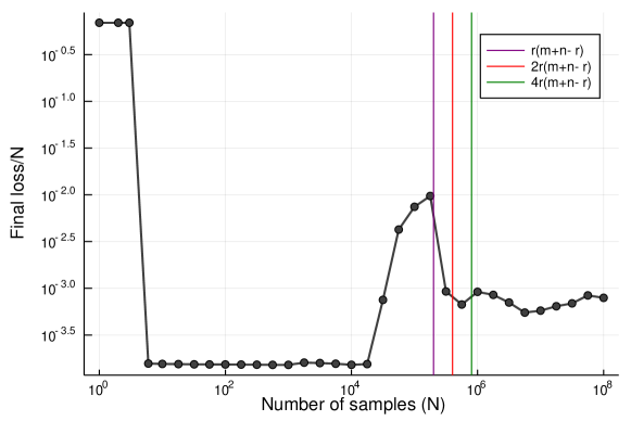
Figure 1. The final loss $\mathcal{L}/N$ attained by sparse proximal gradient descent for a rank-1 generalized low-rank model with no regularization, as a function of the number of samples, $N=\left|\Omega^{\prime}\right|$.

Figure 2. Convergence history of the loss $\mathcal{L}/N$ attained by sparse proximal gradient descent for a rank-10 generalized low-rank model with no regularization, as a function of the number of samples, $N=\left|\Omega^{\prime}\right|$.

4. Semantic analysis of data sets on Kaggle

In this section, we describe a data set curated from the metadata of data sets from Kaggle (kaggle.com). The data set is comprised of metadata from 25,161 datasets that were accessible via the Kaggle Python API (v1.5.6) (Ysteboe, 2019) as of December 4, 2019. For each dataset, we collected 857 unique semantic tags, 44,399 unique file names, and 155,711 column names for each file that comprise the data set. We collected these metadata programmatically through the Kaggle API and preprocessed the data to strip invalid Unicode characters.

Some representative examples are listed in Table 1. We see examples of data quality issues that are typical of collaborative tagging use cases as well as enterprise data catalogues, such as datasets without subject tags, file names without column names, and column names without file names. This data set therefore is a suitable candidate for the topic modeling approach we have described in Section 2.4.

Dataset	tags	filenames	columns
4quant/depth-generation	image data	depth_training_data.npz	-
-lightfield-imaging	leisure
	neural networks
colamas/index1min20190828	-	CA.csv	Close
		HI.csv	High
		NQ.csv	Volume
			… (8 total)
dbahri/wine-ratings	-	test.csv	Portugal
		train.csv	complex
		validation.csv	unoaked
			… (48 total)
insiyeah/musicfeatures			chrome_stft
	music	data.csv	mfcc17
	musical groups	data_2genre.csv	spectral_centroid
			… (25 total)
jackywang529/asdflkjaslj12dsfa	-	-	1
			2
			amanda
			apple (4 total)
mrugankray/license-plates	law	-	-
nltkdata/wordnet	-	-	-
okc35fjh/pearson	education	pearson.xlsx	-

Table 1. Some representative datasets and their metadata from Kaggle.com as collected using version 1.5.6 of the Kaggle API (Ysteboe, 2019).

4.1. Exploratory data analysis

Figure 3 shows the top 10 tags and features in our data set, as well as the cumulative frequencies. It is interesting to note that the tags and features have quite different distributions. While the rank ordering of features shows a power law tail distribution $r^{-\alpha_{f}}$ in the rank $r$ with exponent $\alpha_{f}=2.07\pm 0.01$, the tags are much more heavy-tailed, with a corresponding exponent of $\alpha_{t}=0.853\pm 0.001$. The presence of many rare tags poses a challenge for the standard approach of training an independent classifier for each tag: the classifiers for rare tags do not have sufficient signal in the training data, resulting in poor performance overall.

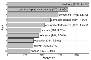
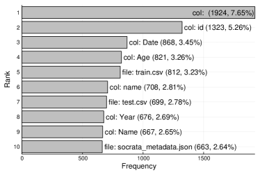
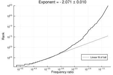
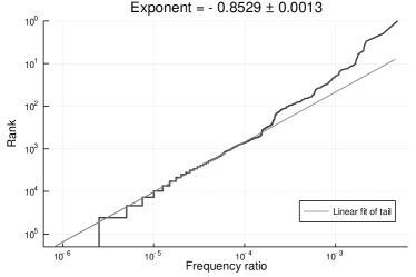
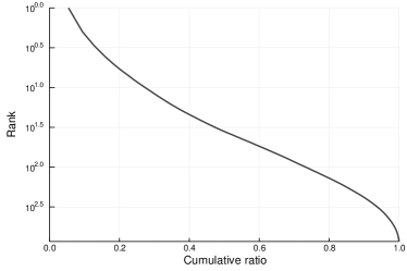
Figure 3. Exploratory analysis of the Kaggle dataset. Top: top 10 most frequent tags (left) and features (right). Middle: rank–frequency distribution of tags and features. Bottom: cumulative distributions of tags and features.

4.2. Topics

Figure 4 shows three typical topics for three different tags of different frequencies of usage: “finance” (used 655 times), “astronomy” (used 70 times), and “cardiology” (used 2 times). For each topic, we show the top five most important and bottom five least important features (first row), and also the the latent strengths (coefficients) of co-occurring with other tags (second row). For example, the “finance” tag correlates positively with the “law and government” tag, as well as the column names “year”, “project_is_approved” and “project_title”, and is negatively correlated with tags “law” and “universities and colleges”, as well as the column name “day”, “sex” and “target”.

Remarkably, the model is able to yield meaningful results using a completely unsupervised technique that has no conception of natural language or semantics. Furthermore, the least important features also semantically very generic, such as the filename “test.csv” or column “date”. In addition, the topics seem to associate with meaningful features, such as variable names suggestive of particle accelerations for the “astronomy” topic. The results suggest that even rare topics can be learned with meaningful signal, which would not have been the case using a more naive approach of training an independent classifier for each topic. With such a long tail of rare topics shown in Figure 3, most of the classifiers would have little meaningful training data to learn from.

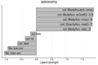
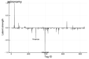
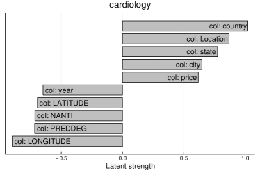
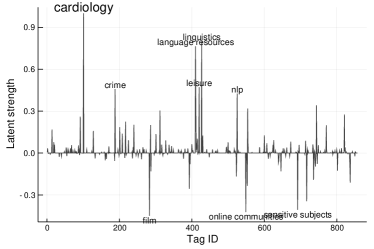
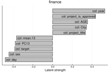
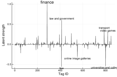
Figure 4. Three representative topics from the GLRM topic model in the Kaggle data set: astronomy (top), cardiology (middle) and finance (bottom). Left: top 5 features and bottom 5 features that are most strongly correlated with the topic. Right: Tags that co-occur with the anchor tag for that topic.

We now describe two additional aspects of our study on the Kaggle data set, the details of which we omit for brevity.

Sparsity in the topic model

Perhaps unsurprisingly, the topic model trained with no sparsity penalty ($\lambda=0$) resulted in a completely dense topic model. Other values of $\lambda=10^{n}$, $n=-3,...,+3$ were also studied. We observed a large increase in sparsity in going from $\lambda=0.01$ to $\lambda=0.1$; the results shown here are presented for $\lambda=0.01$. For large values of $\lambda\geq 10$, the results became effectively nonsensical, with no propensity for label co-occurrence, but also essentially no features associated with the topic either. Thus, the regularization parameter $\lambda$ should be chosen carefully to strike the right balance between sparsity promotion and yielding meaningful results, perhaps using a cross-validation or other hyperparameter tuning strategy.

Non-negativity constraints

We also explored a variant of the GLRM-based topic model with non-negativity constraints, which are straightforward to incorporate using the appropriate proximal operators (Udell et al., 2016). Constraining $Y$ to be non-negative yielded results to what we see for both the toy example of Section 2.5 and the Kaggle data set, with the primary effect of zeroing out uninformative features (rather than assigning them negative weights of evidence in the topic). Constraining $X$ to be non-negative was numerically unstable, yielding $Y$ matrices with large negative and large positive entries. The training loss decreased very slowly in later iterations, suggesting very flat local curvature in the loss surface. These results suggest that allowing both positive and negative entries in $X$ is critical to yield a well-defined topic model, whereas nonnegativity in $Y$ may have some benefit in retraining only the features with positive weights of evidence. This phenomenon may be worth studying in future work.

We conclude this section by discussing limitations and potential extensions of our current study.

Polysemy

As described in Sections 2.3 and 2.4, our current study considers only perfectly monosemic labelled topic models (Definition 2.5). A straightforward approach for handling polysemy would simply be to identify the topics with the largest individual losses, introduce additional topics that share the same anchor label, and retrain the model.

Missing concepts

Missing concepts can be inferred by adding additional columns and rows to $A_{\text{t}}$ that are entirely missing, and seeing if the resulting topic model predicts a meaningful distribution for the new topic. However, expert judgment is still required to evaluate the hypothesized missing concepts.

Taxonomy learning

The topic model does not directly yield any taxonomic structure between the concepts. However, such a taxonomy can be learned using subsumption or hierarchical clustering methods (de Knijff et al., 2013).

5. Conclusions

We have introduced a topic modeling approach to learn the mapping between data concepts and their logical representations in the form of physical metadata such as table names and column names. Our main contribution is to introduce the GLRM-based topic model in Algorithm 1, which makes use of a gauge-transformation approach (as illustrated on LSI in Section 2.3) to define perfectly monosemic labelled topic models as a natural extension of unsupervised topic modeling. The GLRM formulation naturally accommodates incorrect and missing labels, as well as hypothesized sparsity of the conceptual–logical mapping, while being also straightforward to learn at scale using randomized subsampling techniques.

We have shown using a simple example in Sections 2.1 and 2.5 that the results are readily interpretable. At the same time, the method is sufficiently scalable to analyze the metadata of Kaggle.com, with results in Section 4 that show evidence for learning semantically meaningful topics with interpretable features as well as relationships between data concepts. The exact sparsity parameter $\lambda$ should be chosen carefully to yield sparse, interpretable topics. While our results ignore the challenges of polysemy, missing concepts, and taxonomy learning, the further extensions are all theoretically possible and can be studied in future work.

Disclaimer

This paper was prepared for informational purposes by the Artificial Intelligence Research group of JPMorgan Chase & Co and its affiliates (“JP Morgan”), and is not a product of the Research Department of JP Morgan. JP Morgan makes no representation and warranty whatsoever and disclaims all liability, for the completeness, accuracy or reliability of the information contained herein. This document is not intended as investment research or investment advice, or a recommendation, offer or solicitation for the purchase or sale of any security, financial instrument, financial product or service, or to be used in any way for evaluating the merits of participating in any transaction, and shall not constitute a solicitation under any jurisdiction or to any person, if such solicitation under such jurisdiction or to such person would be unlawful.

References

- (1)
- Arora et al. (2012) Sanjeev Arora, Rong Ge, and Ankur Moitra. 2012. Learning topic models - Going beyond SVD. In Proceedings of the 53rd. Symposium on Foundations of Computer Science (FOCS ’12). IEEE, New Brunswick, NJ, 1–10.
- Basel Committee on Banking Supervision (2013) Basel Committee on Banking Supervision. 2013. Principles for effective risk data aggregation and risk reporting.
- Berry et al. (1999) Michael W. Berry, Zlatko Drmač, and Elizabeth R. Jessup. 1999. Matrices, Vector Spaces, and Information Retrieval. SIAM Rev. 41, 2 (1999), 335–362.
- Candès and Plan (2011) Emmanuel J. Candès and Yaniv Plan. 2011. Tight Oracle Inequalities for Low-Rank Matrix Recovery From a Minimal Number of Noisy Random Measurements. IEEE Trans. Inf. Theory 57, 4 (April 2011), 2342–2359.
- Candès and Recht (2009) Emmanuel J. Candès and Benjamin Recht. 2009. Exact Matrix Completion via Convex Optimization. Found. Comput. Math. 9, 6 (3 April 2009), 717–772.
- Conca et al. (2015) Aldo Conca, Dan Edidin, Milena Hering, and Cynthia Vinzant. 2015. An algebraic characterization of injectivity in phase retrieval. Appl. Comput. Harmon. Anal. 38, 2 (March 2015), 346–356.
- Davenport et al. (2014) Mark A. Davenport, Yaniv Plan, Ewout van den Berg, and Mary Wootters. 2014. 1-Bit matrix completion. Inf. Inference 3, 3 (Sept. 2014), 189–223.
- Davenport and Romberg (2016) Mark A. Davenport and Justin Romberg. 2016. An Overview of Low-Rank Matrix Recovery From Incomplete Observations. IEEE J. Sel. Top. Signal Process. 10, 4 (June 2016), 608–622.
- de Knijff et al. (2013) Jeroen de Knijff, Flavius Frasincar, and Frederik Hogenboom. 2013. Domain taxonomy learning from text: The subsumption method versus hierarchical clustering. Data Knowl. Eng. 83 (Jan. 2013), 54–69.
- Deerwester et al. (1990) Scott Deerwester, Susan T. Dumais, George W. Furnas, Thomas K. Landauer, and Richard Harshman. 1990. Indexing by latent semantic analysis. J. Am. Soc. Inf. Sci. 41, 6 (Sept. 1990), 391–407.
- Donoho and Stodden (2003) David Donoho and Victoria Stodden. 2003. When Does Non-Negative Matrix Factorization Give a Correct Decomposition into Parts?. In Proceedings of the 16th. Conference on Neural Information Processing Systems (NIPS ’03). MIT Press, Whistler, Canada, 1141–1148.
- Eldar et al. (2012) Yonina C. Eldar, Deanna Needell, and Yaniv Plan. 2012. Uniqueness conditions for low-rank matrix recovery. Appl. Comput. Harmon. Anal. 33, 2 (Sept. 2012), 309–314.
- Gama et al. (2014) João Gama, Indrė Žliobaitė, Albert Bifet, Mykola Pechenizkiy, and Abdelhamid Bouchachia. 2014. A Survey on Concept Drift Adaptation. ACM Comput. Surv. 46, 4, Article 44 (March 2014), 44 pages.
- Golub and Van Loan (2013) Gene H. Golub and Charles F. Van Loan. 2013. Matrix Computations (3 ed.). Johns Hopkins, Baltimore, MD.
- Gondran and Minoux (2008) Michel Gondran and Michel Minoux. 2008. Graphs, Dioids and Semirings: New Models and Algorithms. Springer, Boston, MA.
- Guy and Tonkin (2006) Marieke Guy and Emma Tonkin. 2006. Folksonomies: Tidying Up Tags?
- Khatri and Brown (2010) Vijay Khatri and Carol V. Brown. 2010. Designing Data Governance. Commun. ACM 53, 1 (Jan. 2010), 148–152.
- Kurucz et al. (2007) Miklós Kurucz, András A. Benczúr, and Károly Csalogány. 2007. Methods for large scale SVD with missing values. In Proceedings of the 11th. Knowledge Discovery and Data Mining Cup and Workshop (KDD Cup ’07). 8.
- Lawton and Sylvestre (1971) William H. Lawton and Edward A. Sylvestre. 1971. Self Modeling Curve Resolution. Technometrics 13, 3 (1971), 617–633.
- Lee and Seung (1999) Daniel D. Lee and H. Sebastian Seung. 1999. Learning the parts of objects by non-negative matrix factorization. Nature 401, 6755 (Oct. 1999), 788–791.
- Northcutt et al. (2019) Curtis G. Northcutt, Lu Jiang, and Isaac L. Chuang. 2019. Confident Learning: Estimating Uncertainty in Dataset Labels. arXiv:1911.00068
- Recht (2011) Benjamin Recht. 2011. A Simpler Approach to Matrix Completion. J. Mach. Learn. Res. 12 (Dec. 2011).
- Recht et al. (2010) Benjamin Recht, Maryam Fazel, and Pablo A. Parrilo. 2010. Guaranteed Minimum-Rank Solutions of Linear Matrix Equations via Nuclear Norm Minimization. SIAM Rev. 52, 3 (5 Aug. 2010), 471–501.
- Riegler et al. (2015) Erwin Riegler, David Stotz, and Helmut Bölcskei. 2015. Information-theoretic limits of matrix completion. In Proceedings of the 2015 IEEE International Symposium on Information Theory (ISIT ’15). IEEE, Hong Kong, 1836–1840.
- Rong et al. (2019) Yi Rong, Yang Wang, and Zhiqiang Xu. 2019. Almost everywhere injectivity conditions for the matrix recovery problem. Appl. Comput. Harmon. Anal. (Sept. 2019), 15.
- Thirring (1997) Walter Thirring. 1997. Introduction to Classical Field Theory. Springer, New York, NY, Chapter 7, 285–328.
- Udell et al. (2016) Madeleine Udell, Corinne Horn, Reza Zadeh, and Stephen Boyd. 2016. Generalized low rank models. Found. Trends Mach. Learn. 9, 1 (23 June 2016), 1–118.
- Vandereycken (2013) Bart Vandereycken. 2013. Low-Rank Matrix Completion by Riemannian Optimization. SIAM J. Optim. 23, 2 (2013), 1214–1236.
- Wang and Strong (1996) Richard Y. Wang and Diane M. Strong. 1996. Beyond Accuracy: What Data Quality Means to Data Consumers. J. Manage. Inf. Syst. 12, 4 (1996), 5–33.
- Wang et al. (2011) Shenghui Wang, Stefan Schlobach, and Michel Klein. 2011. Concept drift and how to identify it. J. Web Semant. 9, 3 (Sept. 2011), 247–265.
- West (2003) Matthew West. 2003. Developing High Quality Data Models. Technical Report 2.1. European Process Industries STEP Technical Liaison Executive.
- Xu (2018) Zhiqiang Xu. 2018. The minimal measurement number for low-rank matrix recovery. Appl. Comput. Harmon. Anal. 44, 2 (March 2018), 497–508.
- Ysteboe (2019) Rebecca Ysteboe. 2019. Kaggle API version 1.5.6. https://github.com/Kaggle/kaggle-api
- Zhu and Xing (2011) Jun Zhu and Eric P. Xing. 2011. Sparse Topical Coding. In Proceedings of the 27th. Conference on Uncertainty in Artificial Intelligence (UAI ’11). AUAI Press, Corvallis, Oregon, 831–838.