Understanding Local Robustness of Deep Neural Networks under Natural Variations

Abstract

Deep Neural Networks (DNNs) are being deployed in a wide range of settings today, from safety-critical applications like autonomous driving to commercial applications involving image classifications. However, recent research has shown that DNNs can be brittle to even slight variations of the input data. Therefore, rigorous testing of DNNs has gained widespread attention.

While DNN robustness under norm-bound perturbation got significant attention over the past few years, our knowledge is still limited when natural variants of the input images come. These natural variants, e.g., a rotated or a rainy version of the original input, are especially concerning as they can occur naturally in the field without any active adversary and may lead to undesirable consequences. Thus, it is important to identify the inputs whose small variations may lead to erroneous DNN behaviors. The very few studies that looked at DNN’s robustness under natural variants, however, focus on estimating the overall robustness of DNNs across all the test data rather than localizing such error-producing points. This work aims to bridge this gap.

To this end, we study the local per-input robustness properties of the DNNs and leverage those properties to build a white-box (DeepRobust-W) and a black-box (DeepRobust-B) tool to automatically identify the non-robust points. Our evaluation of these methods on three DNN models spanning three widely used image classification datasets shows that they are effective in flagging points of poor robustness. In particular, DeepRobust-W and DeepRobust-B are able to achieve an F1 score of up to 91.4% and 99.1%, respectively. We further show that DeepRobust-W can be applied to a regression problem in a domain beyond image classification. Our evaluation on three self-driving car models demonstrates that DeepRobust-W is effective in identifying points of poor robustness with F1 score up to 78.9%.

1 Introduction

Deep Neural Networks (DNNs) have achieved an unprecedented level of performance over the last decade in many sophisticated areas such as image recognition [38], self-driving cars [5] and playing complex games [65]. These advances have also motivated companies to adapt their software development flows to incorporate AI components [3]. This trend has, in turn, spawned a new area of research within software engineering addressing the quality assurance of DNN components [55, 73, 92, 42, 36, 57, 11, 32, 40, 91, 74, 20].

Notwithstanding the impressive capabilities of DNNs, recent research has shown that DNNs can be easily fooled, i.e., made to mispredict, with a little variation of the input data [23, 14, 73]—either adding a norm-bound pixel-level perturbation into the original input [71, 23, 9], or with natural variants of the inputs, e.g., rotating an image, changing the lighting conditions, adding fog etc. [14, 55, 52]. The natural variants are especially concerning as they can occur naturally in the field without any active adversary and may lead to serious consequences [73, 92].

(a) $0\mathrm{°}$, bird

(b) +$6\mathrm{°}$, airplane

(c) +$24\mathrm{°}$, cat

(d) -$9\mathrm{°}$, dog

(e) $0\mathrm{°}$, bird

(f) +$6\mathrm{°}$, bird

(g) +$24\mathrm{°}$, bird

(h) -$9\mathrm{°}$, bird

Figure 1: (a)-(d) A well-trained Resnet model [14] misclassifies the rotated variations of a bird image into three different classes though the original un-rotated image is classified correctly. (e)-(h) The same model successfully classifies all the rotated variants of another bird image from the same test set. The sub-captions consist of rotation degrees and the predicted classes.

While norm-bound perturbation based DNN robustness is relatively well-studied, our knowledge of DNN robustness under the natural variations is still limited—we do not know which images are more robust than others, what their characteristics are, etc. For example, consider Figure 1: although the original bird image (a) is predicted correctly by a DNN, its rotated variations in images (b)-(d) are mispredicted to three different classes. This makes the original image (a) very weak as far as robustness is concerned. In contrast, the bird image (e) and all its rotated versions (generated by the same degrees of rotation) in Figure 1:(f)-(h) are correctly classified. Thus, the original image (e) is quite robust. It is important to distinguish between such robust vs. non-robust images, as the non-robust ones can induce errors with slight natural variations.

Existing literature, however, focuses on estimating the overall robustness of DNNs across all the test data  [14, 88, 4]. From a traditional software point of view, this is analogous to estimating how buggy a software is without actually localizing the bugs. Our current work tries to bridge this gap by localizing the non-robust points in the input space that pose significant threats to a DNN model’s robustness. However, unlike traditional software where bug localization is performed in program space, we identify the non-robust inputs in the data space. As a DNN is a combination of data and architecture, and the architecture is largely uninterpretable, we restrict our study of non-robustess to the input space. To this end, we first quantify the local (per input) robustness property of a DNN. First, we treat all the natural variants of an input image as its neighbors. Then, for each input data, we consider a population of its neighbors and measure the fraction of this population classified correctly by the DNN - a high fraction of correct classifications indicates good robustness (Figure 1:e) and vice versa (Figure 1:a). We term this measure neighbor accuracy. Using this metric, we study different local robustness properties of the DNNs and analyze how the weak, a.k.a. non-robust, points differ characteristically from their robust counterparts. Given that the number of natural neighbors of an image can be potentially infinite, first we performed a more controlled analysis by keeping the natural variants limited to spatially transformed images generated by rotation and translation, following the previous work [14, 88, 4]. Such controlled experiments help us to explore different robustness properties while systematically varying transformation parameters.

Our analysis with three well-known object recognition datasets across three popular DNN models, i.e., a total of nine DNN-dataset combinations, reveal several interesting properties of local robustness of a DNN w.r.t. natural variants:

• The neighbors of a weaker point are not necessarily classified to one single incorrect class. In fact, the weaker the point is its neighbors (mis)classifications become more diverse.

• The weak points are concentrated towards the class decision boundaries of the DNN in the feature space.

Based on these findings, we further develop two techniques (a black-box and a white-box) that can localize the points of poor robustness, thereby providing a means of, input-specific, real-time feedback about robustness to the end-user. Our white-box and black-box detectors can identify weak, a.k.a. non-robust, points with f1 score up to 91.4% and 99.1%, respectively, at neighbor accuracy cutoff 0.75. To further check the generalizability of our technique, we aim to detect weak points w.r.t. a self-driving car application where we generated natural input variants by adding rain and fog. Note that these are more complex image transformations, and also the model works in a regression setting instead of classification. These models take an image as input, and output a driving angle. Our white-box detector can identify weak points with f1 score up to 78.9%.

In summary, we make the following contributions:

• We conduct an empirical study to understand the local robustness properties of DNNs under natural variations.

• We develop a white-box (DeepRobust-W) and a black-box (DeepRobust-B) method to automatically detect weak points.

• We present a detailed evaluation of our methods on three DNN models across three image classification datasets. To check the generalizability of our findings, we further evaluate DeepRobust-W in a setting with non-spatial transformations (i.e., rain and fog), a different task (i.e., regression), and a safety-critical application (i.e., self-driving car). We find that DeepRobust can successfully detect weak points with reasonably good precision and recall.

• We made our code public at https://github.com/AIasd/DeepRobust.

2 Background: DNN Testing

Existing studies have proposed different techniques to generate test data inputs by perturbing input images for a DNN and use them to evaluate the robustness of the DNN. Depending on how the input image is perturbed, the techniques for generating DNN test data can be classified into three broad categories:

i) Adversarial inputs are typically generated by norm-based perturbation techniques [23, 39, 53, 9, 46, 85] where some pixels of an input image ($I$) are perturbed by norm-based distance ($l_{1}$,$l_{2}$ or $l_{\inf}$) such that the distance between the perturbed image and $I$ is $\leq\epsilon$, where $\epsilon$ is a small positive value. These adversarial examples are used to expose the security vulnerabilities of DNNs.

ii) Natural variations are generated through a variety of image transformations, and are used to evaluate the robustness of DNNs under such variations [14, 13, 73]. Sources of these variations include changes in camera configuration, or variations in background or ambient conditions. The transformations simulating these variations could be spatial, such as rotation, translations, mirroring, shear, and scaling on images, or non-spatial transformations, such as changes in the brightness or contrast of an image. Here we first focus on spatial transformations as opposed to adversarial one for two reasons. First, compared with adversarial examples, which is fairly contrived, spatial transformations are more likely to arise in more benign environments. Second, using simple parametric spatial transformations like rotations and translations, it is easier to systematically explore the local robustness properties. Later, to emulate a more natural variation we add fog and rain on the images of self-driving car dataset and evaluate our method’s generalizibility.

iii) GAN-based image generation techniques use Generative Adversarial Network (GAN) to synthesize images. GAN is one class of generative models trained as a minimax two-player game between a generative model and a discriminative model [22]. GAN-based image generation has been successfully used to generate DNN test data instances [92, 93].

Standard Accuracy vs. Robust Accuracy. Standard accuracy measures how accurately an ML model predicts the correct classes of the instances in a given test dataset. Robust, a.k.a. adversarial accuracy, estimates how accurately an ML model classifies the generated variants [76]. In this paper, we adopt a point-wise robust accuracy measure, neighbor accuracy, to quantify the robustness of a DNN for the neighbors around each data point.

3 Methodology

3.1 Terminology

Original Data Point: An original data point represents an original un-modified data instance (image in our case) in the studied dataset. The original data points can come from training, validation, or testing dataset, depending on the experimental setting. In Figure 2, the triangle in the center is an original data point.

Neighbors: Neighbors are images generated by the natural variations, e.g., spatial transformations applied to an original image. Since the transformation parameters are continuous (e.g., degree of rotations), there can be an infinite number of neighbors per image. In Figure 2, the small circles around an original data point represent its neighbors.

Neighbor Accuracy: We define neighbor accuracy as the percentage of its neighbors, including itself, that can be correctly classified by the DNN model. Figure 2 illustrates this; here, red small circles indicate misclassified neighbors, while the green small circles are correctly classified ones. The figure shows that there are only five neighbors per original data point. In the left-hand-side diagram, four out of five neighbors are correctly classified by the given DNN model. If the original data point is correctly classified as well, the neighbor accuracy of the original data is (5/6=) 83.3%. Similarly, in Figure 2 (right), four out of the five neighbors have been misclassified by the model; if the original data point is misclassified, the neighbor accuracy is (1/6=) 16.6%.

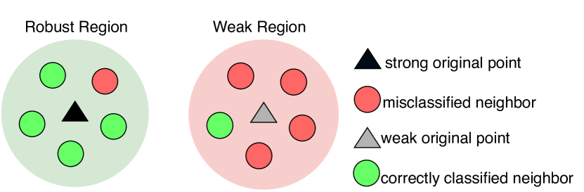
Figure 2: Illustrating our terminologies. The triangles are original points, and the small circles are their neighbors generated by natural variations. The light-green region is robust with higher neighbor accuracy, while the light-red region is vulnerable. The corresponding original points are robust and non-robust accordingly.

Robustness. An original data point is strong, a.k.a. robust, w.r.t. the DNN model under test if its neighbor accuracy is higher than a pre-defined threshold. Conversely, a weak, a.k.a. non-robust, point has the neighbor accuracy lower than a pre-defined threshold. For example, at 0.75 neighbor accuracy threshold, the black triangle in Figure 2 is a strong point, and the grey triangle is a weak point.

A region contains an original point and all of its neighbors. If the original point is strong (weak), we call the corresponding region as a robust (weak) region. In Figure 2, the light green region is robust while the light red region is weak.

Neighbor Diversity: For multi-class classification task, different neighbors of an original point can be mis-classified to different classes. Neighbor Diversity score measures how many diverse classes a point’s neighbors are classified, and is formally computed using Simpson Diversity Index ($\lambda$) [67]: $\lambda=\sum_{i=1}^{k}p^{2}_{i}$ (1)

where $k$ is the total number of possible classes and $p_{i}$ is the probability of an image’s neighbors being predicted to be class $i$. Large Simpson Index means low diversity. Let’s consider we have three possible classes A, B, and C. Assume an image has 4 neighbors. Including the original image, there are 5 images in total. If two of the five images are classified as A, and rest are classified as B, then $\lambda=(2/5)^{2}+(3/5)^{2}+(0/5)^{2}=0.52$. In contrast, if two of them are classified as A, and two are classified as B, and one is classified as C then $\lambda=(2/5)^{2}+(2/5)^{2}+(1/5)^{2}=0.36$. Clearly, the latter case is more diverse and thus, has a lower $\lambda$ score.

Feature Representation: In a DNN, the neurons’ output in each layer capture different abstract representation of the raw input, which are commonly known as features, extracted by the current layer and all the preceding layers. Each layer’s output forms the corresponding feature space. For a given input data point, we consider the output of the DNN’s second-to-last layer as its feature representation or feature vector.

3.2 Data Collection

Neighbor Generation: For the image classification tasks, for each original image point, we generate its neighbors by combining two types of spatial transformations: rotation and translation. We carefully choose these two types as representatives of non-linear and linear spatial transformations, respectively, following Engstrom et al.  [14]. In particular, following them, we generate a neighbor by randomly rotating the original point by t ($\in[-30,30]$) degrees, shifting it by $dx$ (about 10% of the original image’s width i.e. $\in[-3,3]$) pixels horizontally, and shifting it by $dy$ (about 10% of the original image’s height i.e. $\in[-3,3]$) pixels vertically. It should be noted that for image classification it is standard in the literatures [15, 14, 86] to assume that the transformed image has the same label as the original one. As the transformation parameters are continuous, there can be infinite neighbors of an original data point. Hence, we sample $m$ neighbors for each original data point. We explore the impact of $m$ in RQ2.

For the self-driving-car task where the model predicts steering angle, for each original image point, we generate 50% neighbors with rain effect and the rest 50% with fog effects. We adopt a widely used self-driving car data augmentation package, Automold [60], for adding these effects where we randomly vary the degrees of the added effect. For the rain effect, we set “rain_type=heavy" and everything else as default. For the fog effect, we set everything as default.

Estimating Neighbor Accuracy: To compute the neighbor accuracy of a data point for a given DNN model, we first generate its neighbor samples by applying different transformations—spatial for image classification and rain or fog for self-driving-car application. Then we feed these generated neighbors into the DNN model and compute the accuracy by comparing the DNN’s output with the label of the original data point. For self-driving-car application, we follow the technique described in DeepTest [73]. More specifically, if the predicted steering angle of the transformed image is within a threshold to the original image, we consider it as correct. This ensures that any small variations of steering angle are tolerated in the predicted results. We then compute $neighbour\ accuracy=\frac{\#correct\ predictions}{original\ point+\#total\ neighbours}$.

3.3 Classifying Robust vs. Weak Points

We propose two methods, DeepRobust-W and DeepRobust-B, to identify whether an unlabeled input is strong or weak w.r.t. a DNN in real time. If a test image is identified as a weak point, although it may be classified correctly by the pre-trained model, this image is in a vulnerable region where a slight change to this image may cause the pre-trained DNN to misclassify the changed input.

3.3.1 DeepRobust-W: White-box Classifier

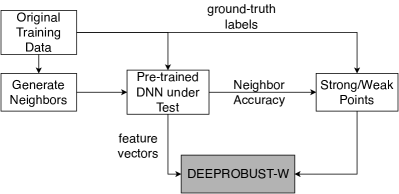
(a) workflow - training

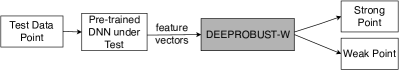
(b) workflow - testing

Figure 3: Workflow of DeepRobust-W

This is a binary classifier designed to classify an image (in particular, image feature vector) as a strong or weak point. Here, we assume that we have white box access to the DNN under test to extract the feature vectors of the input images from the DNN. These feature vectors are given as inputs to DeepRobust-W. Figure 3 shows the workflow.

Training: During training of DeepRobust-W, we first feed all the original training images and their neighbors to the DNN under test. From the DNN outputs, we compute the neighbor accuracy for each data point in the training set and label each point strong/weak depending on whether its neighbor accuracy is higher/lower than a predefined threshold. For each original data point, we also extract the output of the DNN’s second-to-last layer as its feature vector. We use these vectors as inputs to train DeepRobust-W and the outputs are the corresponding strong/weak labels.

Testing: Given a test input, we extract its feature vector by feeding the test image to the DNN under test and then feed the extracted feature vector to the trained DeepRobust-W, which predicts if the input is a strong or weak point.

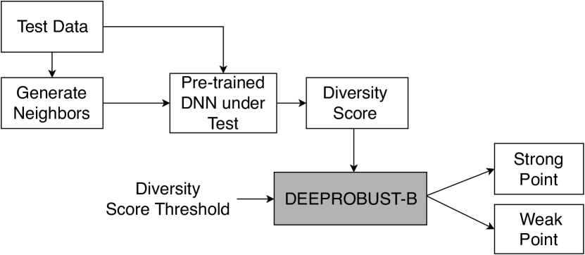
Figure 4: Workflow of DeepRobust-B

3.3.2 DeepRobust-B: Black-box Classifier

This is also a binary classifier that is intended to classify an image to strong/weak point. However, here the user does not have white box access to the DNN under test. Figure 4 shows the workflow.

Given a test input, we first randomly generate some of its neighbors. We then query the DNN under test with all these neighbors and compute the diversity score, as per Equation 2. If the neighbor diversity score (inversely correlated with neighbor diversity) is greater than a given diversity score threshold, the given test input is classified as a strong point; otherwise, a weak point.

Notice that, in this method, we do not need a training step. We only need the diversity score threshold, which can be empirically set using a ground-truth data set. In particular, we first calculate the neighbor accuracy and diversity score of each pre-annotated point. Next, based on a given neighbor accuracy threshold, we identify the weak points, as the ground truth. The highest diversity score among these weak points is chosen as the diversity score threshold.

3.3.3 Usage Scenario

DeepRobust-W/B works in a real-world setting where a customer/user runs a pre-trained DNN model in real-time which constantly receives inputs and wants to test if the prediction of the DNN on a given input can be trusted. DeepRobust-W assumes that the user has white-box access to DNN under test and all the training data used to train the DNN. DeepRobust-W leverages the feature vector and neighbor accuracy of the training data to train the classifier, which can notify the user if the current input is a strong point or weak point. If the input is classified as strong point, the user can give more trust to the original DNN’s prediction. On the other hand, if the point is classified as a weak point, the user may want to be more cautious about the DNN’s prediction and conduct additional inspections.

In the blackbox setting, DeepRobust-B assumes the user does not have white-box access to DNN under test. DeepRobust-B comes with a small overhead of transforming the input multiple times to get some neighbors and querying DNN under test on them to estimate the diversity score.

4 Experimental Design

4.1 Study Subjects

4.1.1 Image Classification

Similar to many existing works [73, 92, 36, 41, 61, 74] on DNN testing, in this work, we use image classification application of DNNs as the basis of our investigation. This is one of the most popular computer vision tasks, where the model tries to classify the objects in an image or video.

Datasets: We conduct our experiments on three image classification datasets: F-MNIST [87], CIFAR-10 [37], and SVHN [89].

• CIFAR-10: consists of 50,000 training and 10,000 testing 32x32 color images. Each image is one of ten digit classes.

• F-MNIST: consists of 60,000 training images and 10,000 testing 28x28 grayscale images. Each image is one of ten fashion product related classes.

• SVHN: consists of 73,257 training images and 26,032 testing images. Each image is a 32x32 color cropped image of house numbers collected from Google Street View images.

Architectures: The popular DNN-based image classifiers are variants of convolutional neural networks (CNN) [28, 79, 38]. Here we study the following three architectures for all the three datasets:

• ResN: Following Engstrom et al. [14], we use ResN model with 4 groups of residual layers with filter sizes 16, 16, 32, and 64, and 5 residual units each.

• VGG: We use the same VGG  architecture as proposed in [66].

• WRN: We use a structure with block type (3, 3) and depth 28 in [90] but replace the widening factor 10 with 2 for less parameters and faster training.

We train all the models from scratch using widely used hyper-parameters and achieve accepted level of validation natural accuracy). When training models on CIFAR-10, we pre-process the input images with random augmentation (random translation with $dx,dy\in[-2,2]$ pixels both horizontally and vertically) which is a widely used preprocessing step for this dataset. When training models on the other two datasets, plain images are directly fed into the models. The natural accuracies and robust accuracies of the models are shown in  Table 1.

Table 1: Study Subjects (values are in percentage)

Dataset	CIFAR-10			SVHN			F-MNIST
Model	VGG	ResN	WRN	VGG	ResN	WRN	VGG	ResN	WRN
nat acc’	89.0	89.3	90.6	94.5	95.3	95.2	93.4	93.5	93.6
rob acc*	75.5	68.5	74.8	78.1	78.9	81.	61.1	63.0	64.2

’Natural accuracy. *Robust accuracy is estimated as the average neighbor accuracy for test data points.

4.1.2 Steering Angle Prediction

We further evaluate DeepRobust-W in a self-driving car application to show that it can be applied into a regression task. These models learn to steer (i.e., predict steering angle) by taking in visual inputs from car-mounted cameras that record the driving scene, paired with the steering angles from a human driver.

Datasets: We use the dataset by Stocco et al. [68], which is collected by the authors driving on three tracks of different environments in the Udacity Simulator [77]. It consists of 37888 central camera training images and 9427 central camera evaluation images. Each image is of size 320x120.

Architectures: We evaluate our method on the three pre-trained DNN models used in [68]: NVIDIA DAVE-2 [6], Epoch [2], and Chauffeur [1]. These models have been used by many previous testing works on self-driving car [55, 73, 68].

4.2 Evaluation

Evaluation Metric. We evaluate both DeepRobust-W and DeepRobust-B for detecting weak points under twelve and nine different DNN-dataset combinations, respectively, in terms of precision, recall, and F1 score. Let us assume that $E$ is the number of weak points detected by our tool and $A$ is the the number of true weak points in the ground truth set. Then the precision and recall are $\frac{|A\cap E|}{|E|}$ and $\frac{|A\cap E|}{|A|}$, respectively. F1 score is a single accuracy measure that considers both precision and recall, and defined as $\frac{2\times precision\times recall}{precision+recall}$. We perform each experiment for two thresholds of neighbor accuracy that defines strong vs. weak points: 0.75 and 0.50.

Baselines. We compare DeepRobust-W and DeepRobust-B with two baselines. One naive baseline (denoted random) is randomly selecting the same number of points as detected by our proposed method to be weak points. Another baseline (denoted top1) is based on prediction confidence score—if the confidence of a data point is higher than a pre-defined cutoff we call it a strong point, weak otherwise. This baseline is based on the intuition that DNNs might not be confident enough to predict the weak points.

5 Results

In this section, we elaborate on our results. In our preliminary experiments, we have two findings regarding neighbor accuracy. First, the neighbor accuracy vary widely across data points and there is a non-trivial number of points having relatively low neighbor accuracy. For example, for all the models trained on CIFAR-10 dataset, 40% of training data and 42% of testing data have neighbor accuracy <0.75, and 16% of training data and 20% of testing data have neighbor accuracy <0.50. These points degrade the aggregated spatial robustness of the model. The same finding holds for the other two datasets. Second, the distribution of neighbor accuracy for a dataset is similar across different models. For CIFAR-10, F-MNIST and SVHN, $60\%$, $76\%$, and $81\%$, respectively, of data points have neighbor accuracy change $<0.2$ across any two models on the same dataset. This implies that a large portion of data points’ neighbor accuracy is independent of the model selected. Detailed results can be found in Appendix 0.A.

The first observation shows that neighbor accuracy is a distinguishable measure for local robustness for the datasets and models we study. The second observation implies that the properties of points of low neighbor accuracy may be similar across models for each dataset. Following these two observations, we dive deeper and explore the characteristics of data points with different neighbor accuracy in RQ1. We then evaluate the performance of DeepRobust-W and DeepRobust-B which are developed based on the observations from RQ1 in RQ2 and RQ3, respectively. Finally, in RQ4, we evaluate the generalizability of our method by applying DeepRobust-W in a regression task for self-driving cars under more complex transformations.

RQ1. What are the characteristics of the weak points?

We explore the characteristics of robust vs. non-robust points in their feature space. In particular, we check the difference in feature representations between: a) robust and non-robust points, and b) points with different degrees of robustness.

RQ1a. Given a well trained model, do the feature representations of robust and non-robust points vary? In this RQ, we first explore how robust (i.e., strong) and non-robust (i.e., weak) data points are distributed in the feature space.

We apply t-SNE[44], a widely used visualization method, to visualize the distribution of points of different neighbor accuracy in the representation space for all three datasets when using ResN as the classifier. Figure 5 shows the visualization of feature vectors from two randomly picked classes with colors indicating the neighbor accuracy of each point. The darker a point’s color is, the lower its neighbor accuracy is. It is evident that most points of low neighbor accuracy tend to be further away from the class center.

(a) CIFAR-10

(b) F-MNIST

(c) SVHN

Figure 5: The t-SNE plots of data points from two randomly chosen classes across three datasets using ResNet. Darker color indicates lower neighbor accuracy.

To numerically verify this observation, first, we define a class center $c_{k}$ for each class $k$ as the median value of the feature vectors of all the points from class $k$. Thus, if $f_{i}$ is the feature of a point at i^th dimension and $\hat{f_{ik}}$ is the median of the i^th dimension features for all the points in class $k$, $c_{k}$ is defined to be $(\hat{f_{1k}},...,\hat{f_{jk}},...,\hat{f_{nk}})$.

The reason we take median rather than mean is that it is a more statistically stable measure and is less likely to be heavily influenced by outliers in the representation space. Then, for every point $p$, we define a ratio: $r^{(p)}=\frac{d^{(p)}_{same\_class}}{d^{(p)}_{nearest\_other\_class}}$, where $d^{(p)}_{same\_class}$ is the distance of the $p$-th point’s feature vector to its own class center and $d^{(p)}_{nearest\_other\_class}$ is the distance of the $p$-th point’s feature vector to the class center of its closest other class. A small $r^{(p)}$ means that the point $p$ is close to its own class center while far from other classes, i.e., $p$ is far from the decision boundary. In contrast, a larger $r^{(p)}$ indicates that the point $p$ is closer to some other classes, i.e., it is closer to the decision boundary.

Table 2: Weak and strong points ratio, and cohen’s d effect size

Dataset	CIFAR-10			SVHN			F-MNIST
Model	ResN	WRN	VGG	ResN	WRN	VGG	ResN	WRN	VGG
Neighbor Accuracy Cutoff=0.5
$r_{w}$	0.915	0.955	1.004	1.046	1.103	0.997	0.746	0.734	0.976
$r_{s}$	0.609	0.584	0.975	0.294	0.309	0.977	0.297	0.293	0.930
d*	1.368	1.736	1.163	2.077	2.428	1.420	1.426	1.312	1.332
Neighbor Accuracy Cutoff=0.75
$r_{w}$	0.778	0.796	0.992	0.604	0.671	0.983	0.516	0.496	0.953
$r_{s}$	0.588	0.558	0.973	0.260	0.274	0.977	0.253	0.257	0.918
d*	0.786	1.040	0.749	0.860	1.111	0.401	0.749	0.642	0.937

*Cohen’s d effect size of 0.20 = small, 0.50 = medium, 0.80 = large, 1.20 = very large, and 2.0 = huge [10, 59].

We then measure the average $r^{(p)}$ among the weak points (denoted as $r_{w}$) and among strong points (denoted as $r_{s}$) for all three datasets across three models. Besides, we also calculate mann-whitney wilocox test[47] and cohen’s d effect size [10] between the two ratios to test if the two ratios indeed have statistically significant difference and how large the difference is.

As shown in Table 2, for both the neighbor accuracy cutoff (0.5 and 0.75), except one setting, the cohen’s d effect size for every setting is larger than 0.50, which implies a medium to very large difference. Besides, for every setting, the mann-whitney wilocox test value (not shown in the table) is smaller than $1e^{-80}$, which implies the difference is indeed statistically significant.

The visualization and numerical results imply that most weak points are close to the decision boundaries between classes. Note that similar observation was also observed by Kim et. al. [36] in case of adversarial perturbation. In particular, they find that adversarial examples tend to be closer to class decision boundaries. In contrast, we focus on spatial robustness and find that spatially non-robust points are closer to decision boundaries.

RQ1b. Given a well trained model, do the feature representations of the data points vary by their degree of robustness? By analyzing the classifications of the neighbors of weak vs. strong points, we observe that the weaker a point is, its neighbors are more likely to be classified in different classes. We quantify this observation by computing diversity of the outputs a point’s neighbor; We adopt Simpson Diversity Index ($\lambda$) [67] as defined in Figure 2.

Table 3: Spearman Correlation between Neighbor Accuracy and Simpson Diversity Index. All coefficients are reported with statistical significance ($p<0.05$).

Dataset	CIFAR-10			SVHN			F-MNIST
Model	ResN	WRN	VGG	ResN	WRN	VGG	ResN	WRN	VGG
corr.coeff.	0.853	0.909	0.946	0.970	0.984	0.983	0.923	0.962	0.8947

Table 3 shows the Spearman correlation between neighbor accuracy and $\lambda$ on the three datasets and three models for each. Note that while calculating the correlation, we remove points with neighbor accuracy 100% since there are many points having 100% neighbor accuracy and tend to bias upward the Spearman Correlation; if we include points with neighbor accuracy 100%, the correlations become even higher. We notice that for any setting, the Spearman Correlation is never lower than 0.853. This indicates that neighbor accuracy and diversity are highly correlated with each other. For example, the bird image in Fig.1a has neighbor accuracy 0.49 and diversity 0.36, while the bird image in Fig.1e has neighbor accuracy 1 and diversity 1. This shows, the classifier tends to be confused about weak points and mispredicts them into many different kinds of classes.

Result 1: In the representation space, weak points tend to lie towards the class decision boundary while the strong points lie towards the center. The weaker an image is, the model tends to be more confused by it, and classify its neighbors into more diverse classes.

RQ2. Can we detect the weak points in a white-box setting?

We explore this RQ using DeepRobust-W, as discussed in Section 3.3.1. DeepRobust-W takes the feature vector of a data point as input and classifies it to a strong/weak point. We implement DeepRobust-W with a simple 4-layer, fully connected neural network architecture with hidden layer dimensions 1500, 1000, and 500, respectively.

Table 4 shows the result. At $0.75$ setting, DeepRobust-W has F1 up to $91.4\%$, with an average of $76.9\%$. At $0.50$ setting, DeepRobust-W detects weak points with average F1 of $61.1\%$, while it can go up to $79.1\%$. DeepRobust-W consistently performs significantly better than the baseline methods.

The top1 has very good precision, since a mis-classified image with low confidence tends to have very poor local robustness. However, there also exist many images that are correctly classified with high confidence yet have poor local robustness. The miss of these points leads the top1 to have very poor recall and thus even worse F1 compared with the random baseline. Our method comes to aid by providing high recall at the same time of decent precision.

Table 4: Performance of DeepRobust-W and the baseline methods for predicting weak points.

dataset	model	method	0.75 neighbor acc.			0.50 neighbor acc.
			f1	tp	fp	f1	tp	fp
CIFAR-10	ResN	ours	0.79	3844	764	0.581	1290	664
		top1	0.376	1218	206	0.182	255	120
		random	0.488	2372	2236	0.233	520	1445
	WRN	ours	0.747	2901	906	0.56	947	610
		top1	0.35	889	222	0.183	189	90
		random	0.395	1534	2273	0.154	261	1296
	VGG	ours	0.654	2222	938	0.493	747	543
		top1	0.439	1070	153	0.266	278	106
		random	0.332	1127	2033	0.132	200	1090
SVHN	ResN	ours	0.755	6814	2530	0.577	1414	674
		top1	0.315	1665	142	0.267	452	122
		random	0.343	3095	6249	0.086	210	1878
	WRN	ours	0.709	5062	2143	0.582	1404	1055
		top1	0.292	1238	130	0.203	275	85
		random	0.28	2000	5205	0.095	229	2230
	VGG	ours	0.595	5214	3367	0.498	1272	911
		top1	0.172	840	67	0.139	221	52
		random	0.341	2986	5595	0.094	240	1943
F-MNIST	ResN	ours	0.914	6034	873	0.791	2144	556
		top1	0.124	428	11	0.039	57	7
		random	0.657	4340	2567	0.263	712	1988
	WRN	ours	0.896	5743	652	0.76	2033	641
		top1	0.144	490	14	0.045	63	8
		random	0.638	4093	2302	0.281	752	1922
	VGG	ours	0.864	6348	1231	0.654	1895	1082
		top1	0.104	392	5	0.028	39	5
		random	0.734	5393	2186	0.295	854	2123

Notice that DeepRobust-W’s performance depends on the training data selection, mainly (a) how many weak vs. strong points are used to train the model, and (b) how many neighbors are generated per point to decide whether it is strong/weak. To investigate the previous one, we assign a weight to each input point, indicating how likely it would be selected to train DeepRobust-W. In particular, for an input $i$, a weight $w_{i}:=\frac{1+(1-n_{i})^{m}\times 100^{m}}{1+100^{m}}$ is computed, where $n$ is its neighbor accuracy, and $m$ is a configurable parameter; with larger $m$, more weak points are sampled, and vice versa. Thus, if $m$ is larger, DeepRobust-W will be trained with more weak points and vice versa.

Table 5A shows the performance: as $m$ increases, the detector trades precision for recall. In this way, choosing different values of $m$, the precision-recall trade-off of the detector can be adjusted according to a user’s need. From a different perspective, this way of oversampling weak points also addresses the potential problem of imbalanced data when the weak points are much less than the strong points.

Table 5: DeepRobust-W performance using different sampling strategies for training

A: with varying number of strong/weak points
dataset	m	prec	recall	tp	fp	f1
CIFAR-10	0	0.660	0.518	1290	664	0.581
	1	0.615	0.599	1490	932	0.607
	2	0.544	0.699	1740	1460	0.612
SVHN	0	0.677	0.502	1414	674	0.577
	1	0.575	0.653	1837	1357	0.612
	2	0.332	0.767	2160	4356	0.463
F-MNIST	0	0.794	0.787	2144	556	0.791
	1	0.746	0.839	2284	777	0.79
	2	0.712	0.871	2372	962	0.783

B: with varying number of neigbours
dataset	#neighbors	prec	recall	tp	fp	f1
CIFAR-10	6	0.662	0.389	967	493	0.49
	12	0.685	0.384	955	440	0.492
	25	0.665	0.502	1250	629	0.572
	50	0.660	0.518	1290	664	0.581
	200	0.683	0.507	1261	585	0.582
SVHN	6	0.723	0.403	1136	436	0.518
	12	0.672	0.527	1483	725	0.59
	25	0.619	0.629	1771	1090	0.624
	50	0.632	0.605	1703	993	0.618
	200	0.667	0.550	1550	774	0.603
F-MNIST	6	0.817	0.727	1981	443	0.77
	12	0.784	0.790	2153	592	0.787
	25	0.773	0.787	2143	629	0.78
	50	0.836	0.727	1981	390	0.778
	200	0.778	0.812	2211	632	0.794

Next, we check how DeepRobust-W’s performance is dependent on the number of sampled neighbors, because a data point can potentially have infinite neighbors. Table 5B shows that the number of neighbors does not have much influence on the performance of the detector once it goes beyond some value (F1 score change less than 3.5 percentage point between 25 and 200 samples) for all the three datasets. Thus, we choose 50 for all of our experiments. For future work, a statistical bound with confidence intervals for neighbor accuracy can be estimated by modeling neighbor accuracy using distributions like folded normal.

Result 2: DeepRobust-W can identify weak points with reasonably high F1 score: on average $76.9\%$, at $0.75$ neighbor accuracy cut-off.

RQ3. Can we identify the weak points in a black-box setting?

We explore this RQ using DeepRobust-B, as discussed in Section 3.3.2. We assume only having access to unlabeled testing data and the model under test as a black-box. To evaluate DeepRobust-B, we spatially transform each test input $m$ times by randomly applying $d\omega\in[-30,+30]$ degrees rotation, $dx\in[-3,+3]$ pixels horizontal translation, and $dy\in[-3,+3]$ pixels vertical translation. We then calculate the output diversity score ($\lambda$) based on Figure 2 and rank the test images based on $\lambda$. Finally, we mark top $k$ images as potential most non-robust points. The parameter $k$ is chosen according to users’ need.

Figure 6: The spearman correlation coeff. between diversity score ($\lambda$) and neighbor accuracy, with varying #neighbors ($m$).

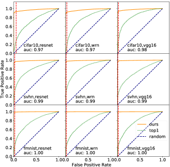
Figure 7: AUC-ROC curve with neighbor accuracy cutoff at 0.75. The red vertical line indicates when the diversity score threshold is chosen from training data.

With each test data, DeepRobust-B queries the model with $m$ neighbors to compute $\lambda$. Since querying the classifier comes with an overhead, our goal is to achieve an optimal accuracy with minimal queries (i.e., $m$). To determine an optimal $m$ value, we explore the spearman correlation between diversity score and neighbor accuracy, with varying $m$, when running ResN on all the three datasets (see Figure 6). The correlation increases as $m$ increases, as with more query $\lambda$ becomes more accurate, and so the neighbor accuracy. We notice that at $m=15$, the correlation coefficients across all the experimental settings reach above 0.8, and the rate of increase begins to slow down significantly. The results for the other two architectures are highly similar. Thus, we set $m=15$ as default for DeepRobust-B.

Next, we evaluate DeepRobust-B’s performance. We plot AUC-ROC by changing $top-k$ at $m=15$ and compare our method with the random baseline and the top1 baseline as before. As shown in Figure 7, our method performs much better than the random baseline. In particular, our proposed method achieves AUC higher than 0.87 for all settings when neighbor accuracy cutoff is 0.5 and 0.97 when neighbor accuracy cutoff is 0.75.

Instead of above ranking based scheme, DeepRobust-B can also be used as a classifier if a diversity threshold is given (see Section 3.3.2). Here, we estimate the threshold using pre-annotated training data.

Table 6: Performance of DeepRobust-B and the baseline methods for predicting weak points.

dataset	model	method	75%			50%
			f1	tp	fp	f1	tp	fp
CIFAR-10	ResN	ours	0.939	4714	257	0.622	1454	801
		top1	0.376	1218	206	0.182	255	120
		random	0.501	2516	2455	0.234	549	1706
	WRN	ours	0.938	3657	171	0.585	986	604
		top1	0.35	889	222	0.183	189	90
		random	0.383	1494	2334	0.182	307	1283
	VGG	ours	0.945	3397	148	0.682	1087	390
		top1	0.439	1070	153	0.266	278	106
		random	0.36	1296	2249	0.153	244	1233
SVHN	ResN	ours	0.956	8371	365	0.67	1845	858
		top1	0.315	1665	142	0.267	452	122
		random	0.336	2944	5792	0.102	280	2423
	WRN	ours	0.963	6827	227	0.718	1602	514
		top1	0.292	1238	130	0.203	275	85
		random	0.275	1950	5104	0.085	191	1925
	VGG	ours	0.976	8608	144	0.779	2138	454
		top1	0.172	840	67	0.139	221	52
		random	0.339	2997	5755	0.102	279	2313
F-MNIST	ResN	ours	0.987	6422	81	0.802	2316	546
		top1	0.124	428	11	0.039	57	7
		random	0.655	4265	2238	0.289	835	2027
	WRN	ours	0.989	6246	70	0.857	2297	360
		top1	0.144	490	14	0.045	63	8
		random	0.631	3987	2329	0.274	736	1921
	VGG	ours	0.991	7078	60	0.847	2393	418
		top1	0.104	392	5	0.028	39	5
		random	0.711	5084	2054	0.277	784	2027

We evaluate precision and recall of DeepRobust-B in the nine DNN-dataset combinations under neighbor accuracy cutoffs 0.5 and 0.75. Table 6 shows the result. At $0.75$ setting, DeepRobust-B has f1 up to $99.1\%$, with an average of $96.5\%$. At $0.50$ setting, DeepRobust-B detects weak points with average f1 of $72.9\%$, while it can go up to $85.7\%$. It consistently produces better estimation than the top1 baseline and the random baseline. This shows that our black-box method can effectively identify weak points.

Note that, generating the spatial transformations and querying the model with it under black box setting is fast. Previous black box methods for adversarial perturbation work in such fashion [26, 51]. For example, using CIFAR-10 , when we use a batch with size 100, the average transformation+query time for one image is $0.031\pm 0.015$ ms. For the other two datasets, the overhead is similar. Thus, to for $m=15$ queries, it takes only $0.465\pm 0.225$ ms, which is a negligible overhead for most real-world DNN based vision applications. This implies that our black-box method can also be used in real time for many applications.

Result 3: Given only black-box access to the DNN classifier, DeepRobust-B can identify weak points with f1 that are much better than those of using top1 method or random method.

RQ4. How generalizable are these findings?

The local robustness issues also exist in more critical applications like self-driving-car. Here we explore more complex transformations, i.e., adding rain and fog to the driving scenes. As shown in Figure 8, among those correctly classified data points, there is a non-trivial portion (45.8%) of them (in the heatmap, more red signified weaker) suffer from low (<0.75) neighbor accuracy.

Note that, here, we test regression models, which take images of driving scenes as inputs and output the corresponding steering angles.

Let a set of outputs predicted by a DNN be denoted by $\{\hat{\theta}_{o1},\hat{\theta}_{o2},...,\hat{\theta}_{on}\}$, and ground truth labels for the original (unmodified) image points be $\{\theta_{1},\theta_{2},...,\theta_{n}\}$. If the difference between predicted steering angle $\hat{\theta}_{oi}$ of a transformed image and the ground truth label of the original image $\theta_{i}$ is above a threshold, we consider it as incorrect.

The threshold $\lambda MSE_{orig}$ is defined following DeepTest’s [73], where $MSE_{orig}=\frac{1}{n}\sum_{i=1}^{n}(\theta_{i}-\hat{\theta}_{oi})^{2}$ . $MSE$ is the Mean Square Error between the outputs and the manual labels, and $\lambda$ is a positive coefficient that is chosen to reflect a user’s tolerance on the deviation. Note that there is no softmax layer (and thus no confidence score) in these regression models so the top1 baseline method cannot be used here.

Figure 8: The t-SNE plot of correctly classified data points from Self-Driving  dataset by the epoch model. data points are colored based on neighbor accuracy.

Table 7 shows the result when $\lambda=3$. At $0.75$ setting, DeepRobust-W has f1 score up to $78.9\%$, with an average of $58.2\%$. At $0.50$ setting, DeepRobust-W detects weak points with an average f1 of $47.9\%$, while it can go as high as $68.2\%$. It consistently produces much better estimation than the random baseline under all the settings. It should be noted that our observation is valid for all the $\lambda$ used in [73] from $\lambda$ equal to 1 to 5. This shows that our proposed method DeepRobust-W can be applied to regression problems with more complex natural transformations.

model	method	0.75 neighbor acc.			0.50 neighbor acc.
		f1	tp	fp	f1	tp	fp
chauffeur	ours	0.417	555	547	0.346	339	384
	random	0.146	194	908	0.096	94	629
epoch	ours	0.789	4354	1112	0.682	2641	1127
	random	0.586	3234	2232	0.411	1592	2176
dave2	ours	0.541	979	471	0.409	475	246
	random	0.193	350	1100	0.121	141	580

Table 7: Performance of DeepRobust-W for predicting weak points of Self-Driving dataset

It should also be noted that it is unrealistic to use DeepRobust-B for this task for two reasons: It is impractical to try different variations of an image in real-time for a self-driving car, which is a time-sensitive application. Further, DeepRobust-B requires the calculation of neighbor diversity score. For a regression problem, the predicted values are continuous, so there is a very low probability for any two predictions being equal. Thus, the neighbor diversity score for every data point will be the same and cannot be used for identifying the weak points.

Result 4: DeepRobust-W can detect weak points of a self-driving car dataset with f1 score up to 78.9%, with an average of 58.2%, at neighbor accuracy cutoff 0.75.

6 Related Work

Adversarial examples. Many works focus on generating adversarial examples to fool the DNNs and evaluate their robustness using pixel-based perturbation [23, 9, 17, 49, 80, 36, 83, 82, 81, 25, 63, 54, 48, 31]. Some other papers [86, 15, 14], like us, proposed more realistic transformations to generate adversarial examples. In particular, Engstrom et al. [14] proposed that a simple rotation and translation can fool a DNN based classifier, and spatial adversarial robustness is orthogonal to $l_{p}$-bounded adversarial robustness. However, all these works estimate the overall robustness of a DNN based on its aggregated behavior across many data points. In contrast, we analyze the robustness of individual data points under natural variations and propose methods to detect weak/strong points automatically.

DNN testing. Many researchers [55, 41, 70, 36, 74, 94, 21, 69, 29, 16] proposed techniques to test DNN. For example, Pei et al. [55] proposed an image transformation based differential testing framework, which can detect erroneous behavior by comparing the outputs of an input image across multiple DNNs. Ferit et al. [16] used fault localization methods to identify suspicious neurons and leveraged those to generate adversarial test cases.

In contrast, others [73, 92, 94, 29, 8, 78, 64] used metamorphic testing where the assumption is the outputs of an original and its transformed image will be the same under natural transformations. Among them, some use a uncertainty measure to quantify some types of non-robustness of an input for prioritizing samples for testing / retraining [8] or generating test cases[78]. We follow a similar metamorphic property while estimating neighbor accuracy and our proposed DeepRobust-B also leverages an uncertainty measure. The key differences are: First, we focus on estimating model’s performance on general natural variants of an input rather than the input itself or only spatial variants. Second, we focus on the task of weak points detection rather than prioritizing / generating test cases. We also give detailed analyses of the properties of natural variants and propose a feature vector based white-box detection method DeepRobust-W. Further, we show that our method works across domains (both image classification and self-driving car controllers) and tasks (both classification and regression). Other uncertainty work complement ours in the sense that we can easily leverage weak points identified by DeepRobust-W and DeepRobust-B to prioritize test cases or generate more adversarial cases of natural variants.

Another line of work [58, 19, 27, 72, 33, 34, 18] estimates the confidence of a DNN’s output. For example, [19] leverages thrown away information from existing models to measure confidence; [27] shows other NN properties like depth, width, weight decay, and batch normalization are important factors influencing prediction confidence. Although such methods can provide a confidence measure per input or its adversarial variants, they do not check its natural robustness property, i.e., with natural variations how will they behave.

DNN verification. There also exist work on verifying properties for a DNN model [56, 83, 30, 62, 12, 7, 24]. Most of them focus on verifying properties on $l_{p}$ norm bounded input space. Recently, Balunovic et al.[4] provides the first verification technique for verifying a data point’s robustness against spatial transformation. However, their technique suffers from scalability issues.

Robust training. Regular neural network training involves the optimization of the loss value for each data point. Robust training of neural network works on minimizing the largest loss within a specific bounded region usually using adversarial examples [81, 35, 50, 84, 83, 15, 45, 75, 43]. While both robust training methods and our work generate variants of data points, instead of training a model with these variants to improve robustness, we leverage them to estimate the robustness of the unseen data points. The relation between robust retraining and our work is thus similar to bug fixing vs. bug detection in traditional software engineering literature.

7 Threats to Validity

We adopt rotation and translation as transformations for image classification tasks and rain and fog effects for the self-driving car task. There are many more natural variations such as brightness, snow effect etc. However, rotation and translation are representative of spatial transformation and used by many paper in evaluating robustness of DNN models[14, 55]. Rain and fog effects are also widely leveraged in many influential studies on testing self-driving cars [55, 73, 92].

Besides, for some of the experiments we did not show all the combinations under both neighbor accuracy cutoffs (i.e. 0.5 and 0.75). However, we note that the observations are consistent and we did not include them purely because of space limitation. Another limitation is that for both DeepRobust-W and DeepRobust-B, we need to decide the number of neighbors to use for training a classifier and estimating $\lambda$, respectively. We mitigate it by selecting the neighbor numbers that give stable performance in terms of precision and recall.

8 Conclusion and Future Work

In this work, we involve the data characteristic into the robustness testing of DNN models. We adopt the concept of neighbor accuracy as a measure for local robustness of a data point on a given model. We explore the properties of neighbor accuracy and find that weak points are often located towards corresponding class boundaries and their transformed versions tend to be predicted to be more diverse classes. Leveraging these observations, we propose a white-box method and a black-box method to identify weak/strong points to warn a user about potential weakness in the given trained model in real-time. We design, implement and evaluate our proposed framework, DeepRobust-W and DeepRobust-B, on three image recognition datasets and one self-driving car dataset (for DeepRobust-W only) with three models for each. The results show that they can effectively identify weak/strong points with high precision and recall.

For future work, other consistency analysis methods [18] e.g. variation ratio, entropy can be tried. We can potentially attain statistical guarantee for our black-box method by modeling the neighbor accuracy distribution and assume certain level of correlation between neighbor accuracy and complexity score. Besides, other definitions of robustness like consistency can be explored. We can also leverage ideas from [8, 78] to easily prioritize test cases or generate more hard test cases based on identified weak points. Further, we can potentially modify existing fixing methods such as [20] targeting the weak points to fix them.

9 Acknowledgement

We thank Mukul Prasad and Ripon Saha from Fujisu US for valuable discussions. This work is supported in part by NSF CCF-1845893 and CCF-1822965.

Appendix

Appendix 0.A More Empirical Results on Characteristics of Spatial Robustness

We first explore the distribution of spatial robustness of the studied data sets w.r.t. three well-trained models. In particular, we explore the variations of spatial robustness: a) across different data points of a given model, b) across different models of a given data point.

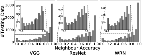
Figure 9: Histogram of neighbor accuracy for CIFAR-10

RQ appendix 1a. Given a well trained model, how spatial robustness changes across different data points? Here, we explore the spatial robustness of each point as captured by its neighbor accuracy. To have a fine-granular understanding, we draw the distribution of neighbor accuracy of data points in both training set and testing set of CIFAR-10 when using VGG, ResN  and WRN  models, respectively, as shown in Figure 9. The histograms show that for all these models, the neighbor accuracy vary widely across data points—most of the data points have very high neighbor accuracy, there is a non-trivial number of points having relatively low neighbor accuracy (40% of training data and 42% of testing data have neighbor accuracy $<$0.75). We call such low accuracy points to be weak or non-robust points. Similarly, for neighbor accuracy $<$0.50, around 16% of training data and 20% of testing data turned out to be weak. These points degrade the aggregated spatial robustness of the model. The same finding also holds for the other two datasets.

The distribution of neighbor accuracy on the training data (not shown in Figure 9) looks similar to that for the testing data. Table 8 further shows that correlation of the number of points in each neighbor accuracy bin between training and testing data is very strong (0.999 to 0.944) with statistical significance ($p<0.05$). Such strong correlation is perhaps not surprising, as training and testing data are taken from the same data distributions.

Table 8: Correlation of spatial robustness (i.e., the number of points per neighbor accuracy bin) between training and testing data

Dataset	CIFAR-10			SVHN			F-MNIST
Model	VGG	ResN	WRN	VGG	ResN	WRN	VGG	ResN	WRN
spearman	0.944	0.979	0.970	0.977	0.997	0.998	0.995	0.983	0.995
pearson	0.998	0.996	0.997	0.998	0.995	0.999	0.995	0.990	0.995

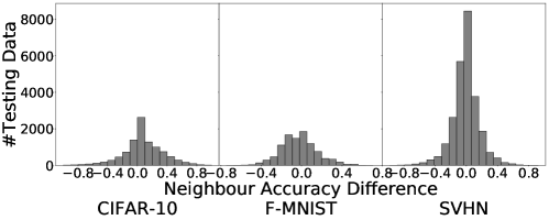
Figure 10: Histogram of per data point neighbor accuracy changes for three datasets from VGG  model to ResN  model across all the three datasets on testing data.

RQ appendix 1b. Given a data point, how spatial robustness changes across different models? Figure 9 shows that the distribution of neighbor accuracy for a dataset looks similar across different models, indicating robustness may be a property of the dataset itself and may not depend on the underlying model architecture. To dig further, for a given dataset, we divide the neighbor accuracy of all data points into 20 equal-sized bins and compute the Spearman and Pearson correlations of the number of points falling into every bin between any two models. To reduce the potential bias induced by the large portion of original points having neighbor accuracy higher than 95%, we also compute the Pearson correlation without them. Table 9 shows that the correlations are very high between any two models for all the three datasets confirming that the overall robustness distribution of a dataset is very similar across different models.

Table 9: Correlation between models in number of points per neighbor accuracy bin

Dataset	Setting	Data	Spearman	Pearson	Pearson
					(w/o last bin)
CIFAR-10	VGG vs ResN	Train	0.980	0.985	0.938
		Test	0.956	0.980	0.920
	VGG vs WRN	Train	0.995	0.996	0.986
		Test	0.977	0.995	0.980
	ResN vs WRN	Train	0.991	0.990	0.980
		Test	0.989	0.986	0.977
SVHN	VGG vs ResN	Train	0.955	0.978	0.979
		Test	0.995	0.983	0.995
	VGG vs WRN	Train	0.977	0.979	0.993
		Test	0.998	0.983	0.994
	ResN vs WRN	Train	0.992	0.986	0.955
		Test	0.998	0.995	0.981
F-MNIST	VGG vs ResN	Train	0.863	0.637	0.969
		Test	0.890	0.627	0.970
	VGG vs WRN	Train	0.877	0.883	0.986
		Test	0.893	0.874	0.969
	ResN vs WRN	Train	0.967	0.901	0.965
		Test	0.979	0.899	0.979

We further examine the per-point variation of robustness across models by analyzing how neighbor accuracy of each data point varies across models. Figure 10 shows that the change is minimal: for CIFAR-10, F-MNIST and SVHN, $60\%$, $76\%$, and $81\%$ of data points have neighbor accuracy change less than $0.2$ across any two models. This implies that a large portion of data points’ neighbor accuracy is independent of the model selected. Note that data points that are non-robust across all the models will not be identified by differential testing techniques as proposed by DeepXplore [55].

Result appendix 1: A non-trivial number of data points (46% at neighbor accuracy $<0.75$) of the whole data set are weak. Robustness seems to be an intrinsic property of the data points and does not vary across models.

References

- [1] Chauffeur model. https://github.com/udacity/self-driving-car/tree/master/steering-models/community-models/chauffeur (2016)
- [2] Epoch model. https://github.com/udacity/self-driving-car/tree/master/steering-models/community-models/cg23 (2016)
- [3] Amershi, S., Begel, A., Bird, C., DeLine, R., Gall, H., Kamar, E., Nagappan, N., Nushi, B., Zimmermann, T.: Software engineering for machine learning: A case study. In: Proceedings of the 41st International Conference on Software Engineering: Software Engineering in Practice. pp. 291–300. ICSE-SEIP ’19, IEEE Press (2019). https://doi.org/10.1109/ICSE-SEIP.2019.00042, https://doi.org/10.1109/ICSE-SEIP.2019.00042
- [4] Balunovic, M., Baader, M., Singh, G., Gehr, T., Vechev, M.: Certifying geometric robustness of neural networks. In: Advances in Neural Information Processing Systems. pp. 15287–15297 (2019)
- [5] Bojarski, M., Del Testa, D., Dworakowski, D., Firner, B., Flepp, B., Goyal, P., Jackel, L.D., Monfort, M., Muller, U., Zhang, J., et al.: End to end learning for self-driving cars. arXiv preprint arXiv:1604.07316 (2016)
- [6] Bojarski, M., Testa, D.D., Dworakowski, D., Firner, B., Flepp, B., Goyal, P., Jackel, L.D., Monfort, M., Muller, U., Zhang, J., Zhang, X., Zhao, J., Zieba, K.: End to end learning for self-driving cars. CoRR abs/1604.07316 (2016), http://arxiv.org/abs/1604.07316
- [7] Bunel, R., Turkaslan, I., Torr, P.H., Kohli, P., Kumar, M.P.: A unified view of piecewise linear neural network verification. In: Proceedings of the 32nd International Conference on Neural Information Processing Systems. p. 4795–4804. NIPS’18, Curran Associates Inc., Red Hook, NY, USA (2018)
- [8] Byun, T., Sharma, V., Vijayakumar, A., Rayadurgam, S., Cofer, D.: Input prioritization for testing neural networks (01 2019)
- [9] Carlini, N., Wagner, D.: Towards evaluating the robustness of neural networks. In: Security and Privacy (SP), 2017 IEEE Symposium on. pp. 39–57. IEEE (2017)
- [10] Cohen, J.: Statistical Power Analysis for the Behavioral Sciences. Lawrence Erlbaum Associates (1988)
- [11] Du, X., Xie, X., Li, Y., Ma, L., Liu, Y., Zhao, J.: Deepstellar: Model-based quantitative analysis of stateful deep learning systems. In: Proceedings of the 2019 27th ACM Joint Meeting on European Software Engineering Conference and Symposium on the Foundations of Software Engineering. p. 477–487. ESEC/FSE 2019, Association for Computing Machinery, New York, NY, USA (2019). https://doi.org/10.1145/3338906.3338954, https://doi.org/10.1145/3338906.3338954
- [12] Ehlers, R.: Formal verification of piece-wise linear feed-forward neural networks. In: International Symposium on Automated Technology for Verification and Analysis. pp. 269–286. Springer (2017)
- [13] Engstrom, L., Tran, B., Tsipras, D., Schmidt, L., Madry, A.: A rotation and a translation suffice: Fooling cnns with simple transformations. arXiv preprint arXiv:1712.02779 (2017)
- [14] Engstrom, L., Tran, B., Tsipras, D., Schmidt, L., Madry, A.: Exploring the landscape of spatial robustness. In: International Conference on Machine Learning. pp. 1802–1811 (2019)
- [15] Engstrom, L., Tran, B., Tsipras, D., Schmidt, L., Mądry, A.: A rotation and a translation suffice: Fooling cnns with simple transformations. In: Proceedings of the 36th international conference on machine learning (ICML) (2019)
- [16] Eniser, H.F., Gerasimou, S., Sen, A.: Deepfault: Fault localization for deep neural networks. In: Hähnle, R., van der Aalst, W. (eds.) Fundamental Approaches to Software Engineering. pp. 171–191. Springer International Publishing, Cham (2019)
- [17] Feinman, R., Curtin, R.R., Shintre, S., Gardner, A.B.: Detecting adversarial samples from artifacts. arXiv preprint arXiv:1703.00410 (2017)
- [18] Gal, Y.: Uncertainty in Deep Learning (2016)
- [19] Gal, Y., Ghahramani, Z.: Dropout as a bayesian approximation: Representing model uncertainty in deep learning. In: Balcan, M.F., Weinberger, K.Q. (eds.) Proceedings of The 33rd International Conference on Machine Learning. Proceedings of Machine Learning Research, vol. 48, pp. 1050–1059. PMLR, New York, New York, USA (20–22 Jun 2016), http://proceedings.mlr.press/v48/gal16.html
- [20] Gao, X., Saha, R., Prasad, M., Roychoudhury, A.: Fuzz testing based data augmentation to improve robustness of deep neural networks. In: Proceedings of the 42nd International Conference on Software Engineering. ICSE 2020, ACM (2020)
- [21] Gerasimou, S., Eniser, H.F., Sen, A., Çakan, A.: Importance-driven deep learning system testing. In: International Conference of Software Engineering (ICSE) (2020)
- [22] Goodfellow, I., Pouget-Abadie, J., Mirza, M., Xu, B., Warde-Farley, D., Ozair, S., Courville, A., Bengio, Y.: Generative adversarial nets. In: Advances in neural information processing systems. pp. 2672–2680 (2014)
- [23] Goodfellow, I.J., Shlens, J., Szegedy, C.: Explaining and harnessing adversarial examples. In: International Conference on Learning Representations (ICLR) (2015)
- [24] Gross, D., Jansen, N., Pérez, G.A., Raaijmakers, S.: Robustness verification for classifier ensembles. In: Hung, D.V., Sokolsky, O. (eds.) Automated Technology for Verification and Analysis. pp. 271–287. Springer International Publishing, Cham (2020)
- [25] Gu, S., Rigazio, L.: Towards deep neural network architectures robust to adversarial examples. In: International Conference on Learning Representations (ICLR) (2015)
- [26] Guo, C., Gardner, J., You, Y., Wilson, A.G., Weinberger, K.: Simple black-box adversarial attacks. In: Chaudhuri, K., Salakhutdinov, R. (eds.) Proceedings of the 36th International Conference on Machine Learning. Proceedings of Machine Learning Research, vol. 97, pp. 2484–2493. PMLR, Long Beach, California, USA (09–15 Jun 2019), http://proceedings.mlr.press/v97/guo19a.html
- [27] Guo, C., Pleiss, G., Sun, Y., Weinberger, K.Q.: On calibration of modern neural networks. In: Precup, D., Teh, Y.W. (eds.) Proceedings of the 34th International Conference on Machine Learning. Proceedings of Machine Learning Research, vol. 70, pp. 1321–1330. PMLR, International Convention Centre, Sydney, Australia (06–11 Aug 2017), http://proceedings.mlr.press/v70/guo17a.html
- [28] He, K., Zhang, X., Ren, S., Sun, J.: Deep residual learning for image recognition. In: Proceedings of the IEEE conference on computer vision and pattern recognition. pp. 770–778 (2016)
- [29] He, P., Meister, C., Su, Z.: Structure-invariant testing for machine translation. In: International Conference of Software Engineering (ICSE) (2020)
- [30] Huang, X., Kwiatkowska, M., Wang, S., Wu, M.: Safety verification of deep neural networks. In: International Conference on Computer Aided Verification. pp. 3–29. Springer (2017)
- [31] Ilyas, A., Santurkar, S., Tsipras, D., Engstrom, L., Tran, B., Madry, A.: Adversarial examples are not bugs, they are features (2019), http://arxiv.org/abs/1905.02175
- [32] Islam, M.J., Nguyen, G., Pan, R., Rajan, H.: A comprehensive study on deep learning bug characteristics. In: Proceedings of the 2019 27th ACM Joint Meeting on European Software Engineering Conference and Symposium on the Foundations of Software Engineering. pp. 510–520. ESEC/FSE 2019, Association for Computing Machinery, New York, NY, USA (2019). https://doi.org/10.1145/3338906.3338955, https://doi.org/10.1145/3338906.3338955
- [33] Jha, S., Raj, S., Fernandes, S., Jha, S.K., Jha, S., Jalaian, B., Verma, G., Swami, A.: Attribution-based confidence metric for deep neural networks. In: Advances in Neural Information Processing Systems. pp. 11826–11837 (2019)
- [34] Jiang, H., Kim, B., Gupta, M.: To trust or not to trust a classifier. In: Advances in Neural Information Processing Systems. pp. 5541––5552 (2018)
- [35] Katz, G., Barrett, C., Dill, D.L., Julian, K., Kochenderfer, M.J.: Reluplex: An Efficient SMT Solver for Verifying Deep Neural Networks, pp. 97–117. Springer International Publishing, Cham (2017)
- [36] Kim, J., Feldt, R., Yoo, S.: Guiding deep learning system testing using surprise adequacy. In: Proceedings of the 41st International Conference on Software Engineering. pp. 1039–1049. IEEE Press (2019)
- [37] Krizhevsky, A.: Learning multiple layers of features from tiny images. University of Toronto (05 2012)
- [38] Krizhevsky, A., Sutskever, I., Hinton, G.E.: Imagenet classification with deep convolutional neural networks. In: Advances in neural information processing systems. pp. 1097–1105 (2012)
- [39] Kurakin, A., Goodfellow, I., Bengio, S.: Adversarial examples in the physical world. arXiv preprint arXiv:1607.02533 (2016)
- [40] Li, Z., Ma, X., Xu, C., Cao, C., Xu, J., Lü, J.: Boosting operational dnn testing efficiency through conditioning. In: Proceedings of the 2019 27th ACM Joint Meeting on European Software Engineering Conference and Symposium on the Foundations of Software Engineering. p. 499–509. ESEC/FSE 2019, Association for Computing Machinery, New York, NY, USA (2019). https://doi.org/10.1145/3338906.3338930, https://doi.org/10.1145/3338906.3338930
- [41] Ma, L., Juefei-Xu, F., Sun, J., Chen, C., Su, T., Zhang, F., Xue, M., Li, B., Li, L., Liu, Y., et al.: Deepgauge: Comprehensive and multi-granularity testing criteria for gauging the robustness of deep learning systems. arXiv preprint arXiv:1803.07519 (2018)
- [42] Ma, S., Liu, Y., Lee, W.C., Zhang, X., Grama, A.: Mode: automated neural network model debugging via state differential analysis and input selection. In: Proceedings of the 2018 26th ACM Joint Meeting on European Software Engineering Conference and Symposium on the Foundations of Software Engineering. pp. 175–186. ACM (2018)
- [43] Ma, X., Li, B., Wang, Y., Erfani, S.M., Wijewickrema, S., Schoenebeck, G., Song, D., Houle, M.E., Bailey, J.: Characterizing adversarial subspaces using local intrinsic dimensionality. In: International Conference on Learning Representations (ICLR) (2018)
- [44] van der Maaten, L., Hinton, G.: Visualizing data using t-SNE. Journal of Machine Learning Research 9, 2579–2605 (2008), http://www.jmlr.org/papers/v9/vandermaaten08a.html
- [45] Madry, A., Makelov, A., Schmidt, L., Tsipras, D., Vladu, A.: Towards deep learning models resistant to adversarial attacks. In: International Conference on Learning Representations (ICLR) (2018)
- [46] Madry, A., Makelov, A., Schmidt, L., Tsipras, D., Vladu, A.: Towards deep learning models resistant to adversarial attacks. In: International Conference on Learning Representations (ICLR) (2018)
- [47] Mann, H.B., Whitney, D.R.: On a test of whether one of two random variables is stochastically larger than the other. Annals of Mathematical Statistics 18(1), 50–60 (1947)
- [48] Mao, C., Zhong, Z., Yang, J., Vondrick, C., Ray, B.: Metric learning for adversarial robustness. In: Advances in Neural Information Processing Systems. pp. 478–489 (2019)
- [49] Metzen, J.H., Genewein, T., Fischer, V., Bischoff, B.: On detecting adversarial perturbations. In: International Conference on Learning Representations (ICLR) (2017)
- [50] Mirman, M., Gehr, T., Vechev, M.: Differentiable abstract interpretation for provably robust neural networks. In: International Conference on Machine Learning. pp. 3575–3583 (2018)
- [51] Moon, S., An, G., Song, H.O.: Parsimonious black-box adversarial attacks via efficient combinatorial optimization. In: Chaudhuri, K., Salakhutdinov, R. (eds.) Proceedings of the 36th International Conference on Machine Learning. Proceedings of Machine Learning Research, vol. 97, pp. 4636–4645. PMLR, Long Beach, California, USA (09–15 Jun 2019), http://proceedings.mlr.press/v97/moon19a.html
- [52] Ozdag, M., Raj, S., Fernandes, S., Velasquez, A., Pullum, L., Jha, S.K.: On the susceptibility of deep neural networks to natural perturbations. In: AISafety@IJCAI (2019)
- [53] Papernot, N., McDaniel, P., Jha, S., Fredrikson, M., Celik, Z.B., Swami, A.: The limitations of deep learning in adversarial settings. In: 2016 IEEE European Symposium on Security and Privacy (EuroS&P). pp. 372–387. IEEE (2016)
- [54] Papernot, N., McDaniel, P., Wu, X., Jha, S., Swami, A.: Distillation as a defense to adversarial perturbations against deep neural networks. In: Security and Privacy (SP), 2016 IEEE Symposium on. pp. 582–597. IEEE (2016)
- [55] Pei, K., Cao, Y., Yang, J., Jana, S.: Deepxplore: Automated whitebox testing of deep learning systems. In: Proceedings of the 26th Symposium on Operating Systems Principles. pp. 1–18. ACM (2017)
- [56] Pei, K., Cao, Y., Yang, J., Jana, S.: Towards practical verification of machine learning: The case of computer vision systems. arXiv preprint arXiv:1712.01785 (2017)
- [57] Pham, H.V., Lutellier, T., Qi, W., Tan, L.: Cradle: Cross-backend validation to detect and localize bugs in deep learning libraries. In: Proceedings of the 41st International Conference on Software Engineering. p. 1027–1038. ICSE ’19, IEEE Press (2019). https://doi.org/10.1109/ICSE.2019.00107, https://doi.org/10.1109/ICSE.2019.00107
- [58] Qiu, X., Meyerson, E., Miikkulainen, R.: Quantifying point-prediction uncertainty in neural networks via residual estimation with an i/o kernel. In: International Conference on Learning Representations (2020), https://openreview.net/forum?id=rkxNh1Stvr
- [59] Sawilowsky, S.: New effect size rules of thumb. Journal of Modern Applied Statistical Methods 8, 597–599 (11 2009). https://doi.org/10.22237/jmasm/1257035100
- [60] Saxena, U.: Automold. https://github.com/UjjwalSaxena/Automold–Road-Augmentation-Library/
- [61] Sen, K., Marinov, D., Agha, G.: CUTE: A concolic unit testing engine for C. In: FSE (2005)
- [62] Seshia, S.A., Desai, A., Dreossi, T., Fremont, D.J., Ghosh, S., Kim, E., Shivakumar, S., Vazquez-Chanlatte, M., Yue, X.: Formal specification for deep neural networks. In: International Symposium on Automated Technology for Verification and Analysis. pp. 20–34. Springer (2018)
- [63] Shaham, U., Yamada, Y., Negahban, S.: Understanding adversarial training: Increasing local stability of neural nets through robust optimization. arXiv preprint arXiv:1511.05432 (2015)
- [64] Shankar, V., Dave, A., Roelofs, R., Ramanan, D., Recht, B., Schmidt, L.: A systematic framework for natural perturbations from videos (06 2019)
- [65] Silver, D., Huang, A., Maddison, C.J., Guez, A., Sifre, L., van den Driessche, G., Schrittwieser, J., Antonoglou, I., Panneershelvam, V., Lanctot, M., Dieleman, S., Grewe, D., Nham, J., Kalchbrenner, N., Sutskever, I., Lillicrap, T., Leach, M., Kavukcuoglu, K., Graepel, T., Hassabis, D.: Mastering the game of go with deep neural networks and tree search. Nature 529, 484–503 (2016), http://www.nature.com/nature/journal/v529/n7587/full/nature16961.html
- [66] Simonyan, K., Zisserman, A.: Very deep convolutional networks for large-scale image recognition. In: International Conference on Learning Representations (ICLR) (2015)
- [67] SIMPSON, E.H.: Measurement of diversity. Nature 163(4148), 688–688 (1949), https://doi.org/10.1038/163688a0
- [68] Stocco, A., Weiss, M., Calzana, M., Tonella, P.: Misbehaviour prediction for autonomous driving systems. In: Proceedings of 42nd International Conference on Software Engineering. p. 12 pages. ICSE ’20, ACM (2020)
- [69] Stocco, A., Weiss, M., Calzana, M., Tonella, P.: Misbehaviour prediction for autonomous driving systems. In: International Conference of Software Engineering (ICSE) (2020)
- [70] Sun, Y., Wu, M., Ruan, W., Huang, X., Kwiatkowska, M., Kroening, D.: Concolic testing for deep neural networks (2018)
- [71] Szegedy, C., Zaremba, W., Sutskever, I., Bruna, J., Erhan, D., Goodfellow, I., Fergus, R.: Intriguing properties of neural networks. In: International Conference on Learning Representations (ICLR) (2014)
- [72] Teye, M., Azizpour, H., Smith, K.: Bayesian uncertainty estimation for batch normalized deep networks. In: Dy, J., Krause, A. (eds.) Proceedings of the 35th International Conference on Machine Learning. Proceedings of Machine Learning Research, vol. 80, pp. 4907–4916. PMLR, Stockholmsmässan, Stockholm Sweden (10–15 Jul 2018), http://proceedings.mlr.press/v80/teye18a.html
- [73] Tian, Y., Pei, K., Jana, S., Ray, B.: Deeptest: Automated testing of deep-neural-network-driven autonomous cars. In: International Conference of Software Engineering (ICSE), 2018 IEEE conference on. IEEE (2018)
- [74] Tian, Y., Zhong, Z., Ordonez, V., Kaiser, G., Ray, B.: Testing dnn image classifier for confusion & bias errors. In: International Conference of Software Engineering (ICSE) (2020)
- [75] Tramèr, F., Kurakin, A., Papernot, N., Goodfellow, I., Boneh, D., McDaniel, P.: Ensemble adversarial training: Attacks and defenses. arXiv preprint arXiv:1705.07204 (2017)
- [76] Tsipras, D., Santurkar, S., Engstrom, L., Turner, A., Madry, A.: Robustness may be at odds with accuracy. In: International Conference on Learning Representations (ICLR) (2019)
- [77] Udacity: A self-driving car simulator built with Unity. https://github.com/udacity/self-driving-car-sim (2017), online; accessed 18 August 2019
- [78] Udeshi, S., Jiang, X., Chattopadhyay, S.: Callisto: Entropy-based test generation and data quality assessment for machine learning systems. In: 2020 IEEE 13th International Conference on Software Testing, Validation and Verification (ICST). pp. 448–453 (2020)
- [79] Wang, F., Jiang, M., Qian, C., Yang, S., Li, C., Zhang, H., Wang, X., Tang, X.: Residual attention network for image classification. In: Proceedings of the IEEE Conference on Computer Vision and Pattern Recognition. pp. 3156–3164 (2017)
- [80] Wang, J., Dong, G., Sun, J., Wang, X., Zhang, P.: Adversarial sample detection for deep neural network through model mutation testing. In: Proceedings of the 41st International Conference on Software Engineering. p. 1245–1256. ICSE ’19, IEEE Press (2019). https://doi.org/10.1109/ICSE.2019.00126, https://doi.org/10.1109/ICSE.2019.00126
- [81] Wang, S., Chen, Y., Abdou, A., Jana, S.: Mixtrain: Scalable training of formally robust neural networks. arXiv preprint arXiv:1811.02625 (2018)
- [82] Wang, S., Pei, K., Whitehouse, J., Yang, J., Jana, S.: Efficient formal safety analysis of neural networks. In: Proceedings of the 32Nd International Conference on Neural Information Processing Systems. pp. 6369–6379. NIPS’18, Curran Associates Inc., USA (2018), http://dl.acm.org/citation.cfm?id=3327345.3327533
- [83] Wang, S., Pei, K., Whitehouse, J., Yang, J., Jana, S.: Formal security analysis of neural networks using symbolic intervals. USENIX Security Symposium (2018)
- [84] Wong, E., Schmidt, F., Metzen, J.H., Kolter, J.Z.: Scaling provable adversarial defenses. In: Advances in Neural Information Processing Systems. pp. 8400–8409 (2018)
- [85] Xiao, C., Li, B., Zhu, J.Y., He, W., Liu, M., Song, D.: Generating adversarial examples with adversarial networks. In: 27th International Joint Conference on Artificial Intelligence (IJCAI) (2018)
- [86] Xiao, C., Zhu, J.Y., Li, B., He, W., Liu, M., Song, D.: Spatially transformed adversarial examples. In: International Conference on Learning Representations (ICLR) (2018)
- [87] Xiao, H., Rasul, K., Vollgraf, R.: Fashion-mnist: a novel image dataset for benchmarking machine learning algorithms (2017)
- [88] Yang, F., Wang, Z., Heinze-Deml, C.: Invariance-inducing regularization using worst-case transformations suffices to boost accuracy and spatial robustness. In: Advances in Neural Information Processing Systems 32. pp. 14757–14768 (2019)
- [89] Yuval Netzer, T.W., Coates, A., Bissacco, A., Wu, B., Ng, A.Y.: Reading digits in natural images with unsupervised feature learning. In: NIPS Workshop on Deep Learning and Unsupervised Feature Learning (2011)
- [90] Zagoruyko, S., Komodakis, N.: Wide residual networks. In: BMVC (2016)
- [91] Zhang, H., Chan, W.K.: Apricot: A weight-adaptation approach to fixing deep learning models. In: 2019 34th IEEE/ACM International Conference on Automated Software Engineering (ASE). pp. 376–387 (Nov 2019). https://doi.org/10.1109/ASE.2019.00043
- [92] Zhang, M., Zhang, Y., Zhang, L., Liu, C., Khurshid, S.: Deeproad: Gan-based metamorphic autonomous driving system testing. arXiv preprint arXiv:1802.02295 (2018)
- [93] Zhao, Z., Dua, D., Singh, S.: Generating natural adversarial examples. In: International Conference on Learning Representations (ICLR) (2018)
- [94] Zhou, H., Li, W., Kong, Z., Guo, J., Zhang, Y., Zhang, L., Yu, B., Liu, C.: Deepbillboard: Systematic physical-world testing of autonomous driving systems. In: International Conference of Software Engineering (ICSE) (2020)