Measuring Transit Signal Recovery in the Kepler Pipeline IV: Completeness of the DR25 Planet Candidate catalog

Abstract

In this work we empirically measure the detection efficiency of Kepler pipeline used to create the final Kepler Threshold Crossing Event (TCE; Twicken et al., 2016) and planet candidate catalogs (Thompson et al., 2018), a necessary ingredient for occurrence rate calculations using these lists. By injecting simulated signals into the calibrated pixel data and processing those pixels through the pipeline as normal, we quantify the detection probability of signals as a function of their signal strength and orbital period. In addition we investigate the dependence of the detection efficiency on parameters of the target stars and their location in the Kepler field of view. We find that the end-of-mission version of the Kepler pipeline returns to a high overall detection efficiency, averaging a 90–95% rate of detection for strong signals across a wide variety of parameter space. We find a weak dependence of the detection efficiency on the number of transits contributing to the signal and the orbital period of the signal, and a stronger dependence on the stellar effective temperature and correlated noise properties. We also find a weak dependence of the detection efficiency on the position within the field of view. By restricting the Kepler stellar sample to stars with well-behaved correlated noise properties, we can define a set of stars with high detection efficiency for future occurrence rate calculations.

in AAS Journals

1 Introduction

The Data Release 25 (DR25) planet candidate catalog from the NASA Kepler mission (Thompson et al., 2018) represents the culmination of eight years’ worth of analysis. The list of 4,034 planet candidates was generated in a fully automated fashion from the full Kepler observation baseline of nearly four years. Using an automatic classification scheme called the Robovetter, the Threshold Crossing Events (TCEs) generated by the Kepler data reduction pipeline were dispositioned as either planet candidates or false positives. This automation allowed, for the first time, an attempt to quantify the completeness (false negative rate) and reliability (false positive rate) of the catalog. These comprise two of the necessary ingredients for measuring the underlying planet occurrence rates from an observed list of planet candidates.

We have run a series of experiments characterising the completeness of almost all the recent versions of the Kepler pipeline, increasing in scope and complexity with each iteration. The work presented here represents the analysis of the fourth such experiment. Previous results can be found in Christiansen et al. (2016, SOC version 9.2, spanning the full observing baseline), Christiansen et al. (2015, SOC version 9.1, spanning one year of observations), and Christiansen et al. (2013, an early version of SOC version 8.3, spanning one month of observations). Each version of the pipeline has its own strengths and weaknesses, and the measured completeness of the accompanying planet candidate catalogs shows significant variations in each case. Therefore, it is crucial for studies of exoplanet demographics that the completeness model used to analyse a given planet candidate catalog be derived from the corresponding pipeline version. The work presented here and in Christiansen (2017) quantifies the completeness of the pipeline version used to generate the catalog published by Thompson et al. (2018); the corresponding quantification of the Robovetter is presented in Coughlin (2017). Christiansen et al. (2016) accompanies the catalog published by Coughlin et al. (2016); Christiansen et al. (2015) accompanies the catalog published by Mullally et al. (2015); and Christiansen et al. (2013) corresponds to an early version of the code used to produce the catalog published by Rowe et al. (2015). In all previous cases there are important caveats in the careful usage and application of the measured completeness; readers should refer to the relevant citations for additional details. In addition, we note that this work does not quantify the false positive rate nor false alarm rate of the Kepler pipeline; these pieces must be calculated and included separately in occurrence rate calculations.

In Christiansen (2017) and Thompson et al. (2018), we presented an initial analysis of the completeness of the DR25 planet candidate catalog to support calculations of $\eta_{\oplus}$, the frequency of Earth-like planets orbiting stars like the Sun. This early analysis was restricted to producing a single 1-dimensional measure of the detection efficiency as a function of the Multiple Event Statistic (MES) of the transit signal, i.e. its signal strength, for all FGK dwarf stars in the Kepler target list. In this paper we extend that analysis to investigate the completeness of the Kepler pipeline along several additional axes, for use in defining and supporting additional science use cases. The paper is organized as follows: in Section 2, we describe the generation of the DR25 planet candidate catalog. In Section 3, we describe the details and execution of this fourth transit injection experiment, and in Section 4 we explore the results. In Section 5 we discuss the implications, and in Section 6 we summarise the final results.

2 DR25 Planet Candidate Catalog Generation

The DR25 planet candidate catalog was produced by uniformly processing the full, four-year dataset (Quarters 1 through 17) through Science Operations Center (SOC) pipeline version 9.3 to produce a list of Threshold Crossing Events (TCEs), described by Twicken et al. (2016). The TCEs were then evaluated by the Robovetter (Coughlin et al., 2016; Thompson et al., 2018), and dispositioned into planet candidates or false positives. In order to empirically recover the detection efficiency of the process—the likelihood a given planet signal will be correctly identified and dispositioned as a planet candidate—we can replicate the process with a suite of known ‘ground-truth’ signals, and analyse their outcomes. We summarise the pipeline and Robovetter processes in the Appendix, with particular emphasis on updates compared to the previous planet candidate catalogs.

3 Pixel-Level Transit Injection

In order to characterize the pipeline detection efficiency, we have performed several distinct transit injection experiments. These largely fall into two categories: pixel-level transit injection (PLTI) and flux-level transit injection (FLTI). For PLTI experiments, simulated transit signals are injected into the calibrated pixels, before the aperture photometry time series is constructed and cotrended. This allows the total detection efficiency loss to be determined through the photometric and search portions of the pipeline. However, PLTI is computationally expensive, since it run most of the pipeline modules. As a result, these PLTI experiments are limited to one injected planetary signal per target star, but include all available target stars. Hence, PLTI provides an average detection efficiency over a set of stars. Knowing that the stars are not all ‘average’, a series of FLTI experiments were also conducted. For FLTI, the transit signal is injected into the cotrended flux time series within the Transiting Planet Search (TPS) module of the pipeline, and the signal detection algorithm is performed over a restricted portion of the period search space focused on the period of the injected signal (Burke & Catanzarite, 2017a). For ‘deep’ FLTI experiments, we chose a small subset ($\sim$100) of stars and performed $\sim$600,000 injection and recovery experiments for each star. For ‘shallow’ FLTI experiments, we chose a larger subset ($\sim$30,000) of stars and performed $\sim$2,000 injection and recovery experiments for each star. These tests determined when and how individual stars can deviate from the average detection efficiency measured by PLTI. This document describes the PLTI experiment only; the FLTI products are documented separately in Burke & Catanzarite (2017a) and examples of using FLTI products to measure detection efficiency are discussed in Burke & Catanzarite (2017b).

For the PLTI experiment described here, we inject simulated transit and eclipse signals into the calibrated pixels of 190,128 targets covering the entire focal plane. These injections fell into three distinct categories, each designed for a specific use case: 146,295 targets were injected with planet-like signals at the target location on the CCD, thereby mimicking a planet orbiting the specified target; 33,978 targets were injected with planet-like signals at a location slightly offset from the nominal target location, thereby mimicking a blended eclipsing binary; and 9,856 targets were injected with eclipsing-binary-like signals (having both primary and secondary eclipses) at the target location on the CCD. The latter two groups were generated to test the Robovetter’s ability to discriminate between various kinds of false positives (for a detailed analysis, see Coughlin, 2017), and are made available along with the first group for the community to test their own algorithms. The analysis described in this work will be restricted to the on-target planet-like signals in the first group, and to the completeness of the Kepler pipeline, not the subsequent Robovetter stage. To generate the simulated transit signals we use the DR25 Q1–Q17 stellar parameters provided by Mathur et al. (2017). An updated set of stellar parameters was released by Berger et al. (2018) during this analysis, but was not found to systematically change the conclusions.

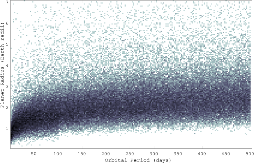
Figure 1: A density distribution of simulated planet signals injected on-target, in planet radius and orbital period space (truncated at 7$R_{\oplus}$). The injections are clustered around the pipeline signal-to-noise threshold, which moves to larger radii for longer periods, in order to examine the transition from detection to non-detection by the pipeline.

For non-M-dwarf targets, each injected signal was generated as follows. First, the orbital period was drawn from a uniform range in period spanning 0.5–500 days. The planet radius was then chosen such that the resulting MES spanned the range 0–20, bracketing the pipeline transition from fully complete (100% signal recovery) to fully incomplete (0% recovery). To estimate the MES for a given injected signal we take into account the stellar radius, orbital period, planet radius, an average Combined Differential Photometric Precision (rmsCDPP; Jenkins et al., 2010a; Christiansen et al., 2012), the dilution of the signal by additional light in the photometric aperture, and the duty cycle of the observations (discarding gapped cadences and de-weighted cadences with weights $<0.5$. We note that this process resulted in some unphysically large radii, but ultimately 50% of the injected planets have radii $<2R_{\oplus}$ and 90% have radii $<40R_{\oplus}$. The orbital eccentricity was fixed at 0, and the impact parameter was drawn from a uniform range spanning 0–1. We also note that, in general, the MES that we estimate for the signal prior to its injection in the light curve will not equal the measured MES. We estimate the MES using a single rmsCDPP value, which is the average noise over the light curve—the actual data points into which the signal is injected may have higher or lower levels of local noise. Figure 2 shows the value of the measured MES compared to the estimated MES; the median value is 0.95, with a standard deviation of 0.15. The overall reduction in the measured MES is at least partly due to the average timing mismatch between the injected period, epoch, and transit duration and the finite grid of periods, epochs, and transit durations over which the pipeline searches (see, e.g Jenkins et al., 1996, 2010b).

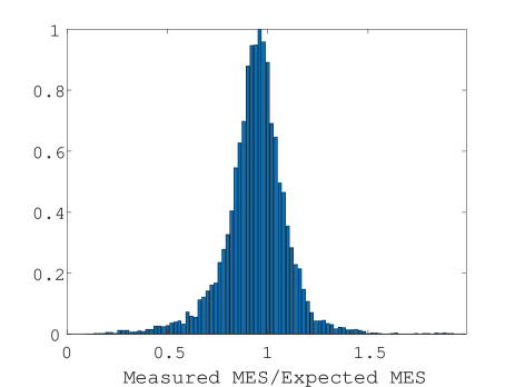
Figure 2: A histogram of the values of the measured MES of the successfully recovered injected signals compared to the estimated MES of the signal prior to injection.

For the M-dwarf targets, where the habitable zone is much closer to the star, we concentrated the injected signals over a smaller period range. For the 3,809 targets with $2400K\leq T_{\rm eff}\leq 3900K$ and $log\rm{g}\geq 4$, the orbital periods were selected from a uniform range spanning 0.5–100 days. Given the stellar radii, noise properties, and orbital periods, this resulted in a smaller injected planet radius distribution than the remainder of the targets, with 50% of the injected planets having radii $<0.92R_{\oplus}$ and 90% have radii $<1.7R_{\oplus}$.

4 Results

The full table of parameters for the injected signals, and if they were recovered, the parameters of the recovered signal, is available at the NASA Exoplanet Archive. All three types of injected signal are included (planet injected on-target, planet injected off-target, and EB injected on-target); for the remainder of this section we focus solely on analysis of the on-target planet signal injections. Of the 146,295 planets, 45,281 were successfully recovered by the pipeline, as shown in Figure 1. We note here that many signals were injected below the signal detection threshold for the express purpose of exploring the transition region from detection to non-detection. For these purposes, ‘success’ is defined by the ephemeris-matching algorithm described in Section 6.2 of Thompson et al. (2018). This incorporates both a period tolerance and a check on the number of transit events, and allows for detections with periods that differ by half/double or a third/thrice the injected period. In the remainder of this Section we explore the detection efficiency of the pipeline with respect to several variables.

4.1 Orbital Period

There is an expected drop in detection efficiency at longer periods due simply to the window function of the observations—beyond some period, meeting the minimum number of transits required for detection becomes less and less likely. For SOC version 9.3, there is an additional penalty applied during TPS to signals with only three contributing transits (see Section 9.4.4.1 of Jenkins et al., 2017). The top panel of Figure 3 shows the detection efficiency of the pipeline as a function of the number of transits contributing to the detection. For the 77,860 targets with at least four transits with durations shorter than 15 hours (the longest duration searched by the pipeline), we assess the fraction of injected signals that are recovered as a function of the number of contributing transits. As we have done in previous work (Christiansen et al., 2013, 2015, 2016), we analyse the detection efficiency in each bin as a function of the expected MES, fitting a $\Gamma$ cumulative distribution function of the form

$$p=F(x|a,b)=\frac{c}{b^{a}\Gamma(a)}\int\limits_{0}^{x}t^{a-1}e^{-t/b}dt$$ (1)

normalized to the value ($c$) at MES = 15. The additional penalty for having only three transits is clear, and has subsequently been incorporated in the generation of the window function (Burke & Catanzarite, 2017c). For the period analysis performed here we only consider injections with four or more transits. We find a remaining dependence of the detection efficiency on orbital period, shown in the middle panel of Figure 3. From 0–300 days there is little change in the overall detection efficiency, barring a small drop in sensitivity in the 0–50 day bin due to the known behavior of the harmonic fitter removing signals at short periods (Christiansen et al., 2013, 2015). For periods longer than 300 days the detection efficiency falls off slightly, from 95–96% at the shorter periods to 87–91% at the longest periods. This is an important caveat for those calculating occurrence rate in this interesting long-period parameter space. Given the dependence of the detection efficiency on orbital period for periods longer than 300 days, we recommend determining the detection efficiency over the period range of interest for a given occurrence rate calculation, rather than relying on the ensemble average detection efficiency, and to pay particular attention to the window function.

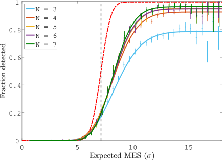
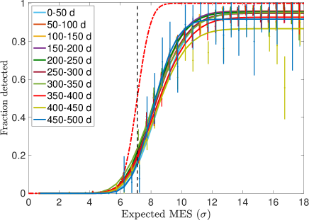
Figure 3: Upper: The 1-dimensional detection efficiency of the pipeline calculated in different numbers of transits ($N$) contributing to the MES. The curves are $\Gamma$ cumulative distribution functions fit to the data. The binomial uncertainties on the data in each bin are shown with small horizontal offsets for clarity. The black dashed line shows the 7.1-$\sigma$ detection threshold of the pipeline, and the red dashed line shows the hypothetical perfect performance of the pipeline for pure white noise. Middle: As above, but calculated for different orbital period ranges. Lower: As above, but calculated for different ranges of stellar effective temperature.

4.2 Stellar Properties

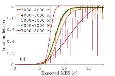
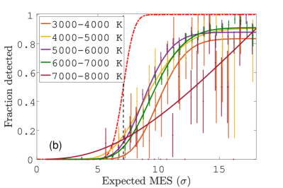
Figure 4: As for Figure 3, but calculated for different ranges in stellar effective temperature. Left: Stars with low (CDPP${}_{\rm L}<-0.2$. Right: Stars with high (CDPP${}_{\rm L}>0.0$.)

The Kepler pipeline measures the noise in a given time series using the Combined Differential Photometric Precision (CDPP; Christiansen et al., 2012). The CDPP is calculated at each data point in the time series for a set of 14 different trial transit durations, and is equivalent to the effective white noise seen by a transit pulse of that duration. An average root-mean-square CDPP (rmsCDPP) value is calculated for each time series and transit duration. For a time series that is dominated by white noise, we expect the rmsCDPP to decrease with increasing transit duration, i.e. for a transit duration that is twice as long, and integrating over twice as many data points, we expect the rmsCDPP to be reduced by a factor of $\sqrt{2}$. Therefore, we can use the change in the rmsCDPP as a function of increasing transit duration to track how well the noise for a given time series is approximated by white noise. We refer to this as the CDPP slope (see Section 3.1 of Burke & Catanzarite, 2017a, for details); it is calculated for short (2–4.5 hr) and long (7.5–15 hr) transit durations, and provided as part of the Kepler stellar parameters at the NASA Exoplanet Archive (Akeson et al., 2013). A simulated transit signal will reach the same SNR in two different light curves if they have the same CDPP. However, if they have different CDPP slopes the ability of the pipeline to extract the transit signal from within the correlated noise is impacted. Burke & Catanzarite (2017a) found previously that the long CDPP slope (CDPP_L) was the most useful discriminator, and the following analysis is based on CDPP_L. CDPP_L tracks the SNR of the stellar variability amplitude on rotation period and some pulsation period time-scales. In order to visualise how CDPP_L represents the noise in the data, we show in Figure 5 light curves of targets with negative CDPP_L (left) and positive CDPP_L (right). The stars in the right panel have increasing rmsCDPP values with increasing trial transit durations, due to the longer transit durations encompassing a higher amplitude of intrinsic stellar variability. On the other hand, the stars in the left panel have decreasing rmsCDPP values with increasing trial transit durations, as the noise bins down as expected for predominately white noise.

Figure 4 shows the detection efficiency of the pipeline broken out by stellar effective temperature for stars with low (CDPP${}_{\rm L}<-0.2$, left panel) and high (CDPP${}_{\rm L}>0.0$, right panel) levels of correlated noise. For this analysis, we have limited the stellar sample to stars with log$g>4.0$, to injections with four or more transits (in order to remove the confounding factor of the detection efficiency on the number of transits discussed in Section 4.1), and with injected transit durations shorter than 15 hours. This leaves 91,672 targets with on-target simulated planet signals. Figure 4 shows that for stars with low levels of correlated noise, those with stellar effective temperatures between 4000–7000 K (roughly FGK stars) have a well-behaved detection efficiency. For cooler dwarfs, the detection efficiency drops off slightly, plateauing at 92% compared to $\sim$96% for the FGK stars. For hotter stars, the detection efficiency drops off somewhat more, although the number of recovered injections (166) is too low for a robust analysis. This decline in detection efficiency for non-FGK stars was also noted in earlier versions of the pipeline (Christiansen et al., 2015). We note that the decrease in detection efficiency for the larger stars is not related to their larger stellar radii relative to the injected planet radii, as this has been accounted for when injecting the planets and calculating the expected MES. We examined the effect of using the updated Gaia DR2 stellar parameters of Berger et al. (2018) here and found that the stellar temperature agreement between the two sets of parameters was very high—for the range of stellar properties examined here, $T_{\rm eff,Kep}=0.9998\pm 0.0027\times T_{\rm eff,Gaia}$, where $T_{\rm eff,Kep}$ and $T_{\rm eff,Gaia}$ are the stellar effective temperature from the Kepler DR25 stellar catalog and Gaia DR2, respectively.

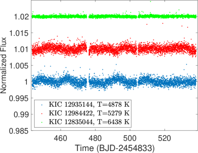
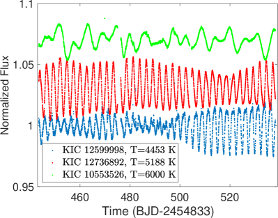
Figure 5: Left: Quarter 5 light curves of a selection of targets with CDPP${}_{\rm L}<-0.3$. Right: The same for targets with CDPP${}_{\rm L}>0.1$. Note the difference in the y axes.

The picture is qualitatively similar but quantitatively lower for stars with high levels of correlated noise. The right panel of Figure 4 shows how the pipeline detection efficiency depends on stellar effective temperature for a sample of stars with positive CDPP_L values. The 4000-7000 K targets still have the highest detection efficiency compared to the very cool and very hot stars, but the overall detection efficiency is reduced by the presence of the correlated noise. This is demonstrated further in Figure 6, which shows how the detection efficiency changes for a range of CDPP_L values over the full sample. For the stars with lower correlated noise (negative CDPP_L values), the behaviour is as expected, plateauing at 97%. For the stars with higher levels of correlated noise (e.g. intrinsic stellar variability) the detection efficiency falls, plateauing at 90%.

As noted earlier, there is a correlation between the stellar temperature and the stellar noise properties. Cooler stars are more active, with more starspot and flaring activity. Figure 7 shows the distribution of CDPP_L values as a function of stellar effective temperature. The two peaks in the lower panel around 3200 K and 4100 K are artifacts of the available targets in those temperature regions, but it is clear that the bulk of the well-behaved (low correlated noise, negative CDPP_L values) are found from 5000–6500 K. The light curves in the right panel of Figure 5 are relatively well-behaved targets across the temperature range, with CDPP${}_{\rm L}<-0.3$, and the light curves in the left panel are targets with much higher levels of correlated noise, with CDPP${}_{\rm L}>0.1$, demonstrating the light curve morphology differences in these two populations. One way to select a stellar sample with a uniformly high detection efficiency is to restrict the selection to those targets with negative CDPP_L values; this eliminates 27,450 of the original 146,295 targets.

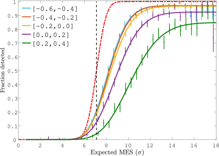
Figure 6: As for Figure 3, but calculated for different ranges in the long CDPP slope (CDPP_L).

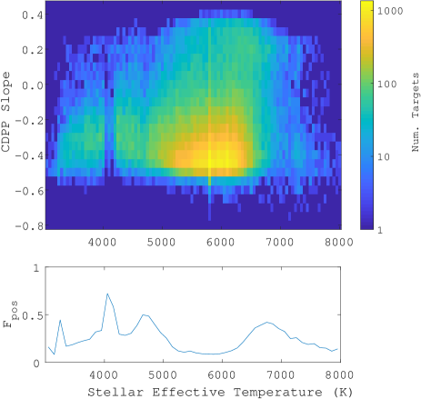
Figure 7: Upper: The distribution of CDPP_L values as a function of stellar effective temperature. The bulk of the Kepler targets are well-behaved solar-like stars. Lower: The fraction of stars with positive CDPP_L values as a function of stellar effective temperature. Stars cooler than $\sim$5000 K and hotter than $\sim$6500 K are more likely to have higher levels of correlated noise in their light curves.

In addition we examine the detection efficiency as a function of stellar magnitude. Figure 8 shows how the detection efficiency varies as a function of magnitude. It is somewhat lower for the saturated targets ($K_{p}<12$), which plateau around 91–93%, rising for the moderately bright targets ($13<Kp<16$), which plateau closer to 95–97%), and dropping significantly for the small number of fainter targets ($K_{p}>16$), reaching only 81%. The behavior at the bright end can be understood by using CDPP_L as a measure of the correlated noise in the light curves. Saturated targets typically have larger apertures to capture the bleed from the electrons that overfill the well depth. These stars have the potential for both pointing-correlated changes in flux if the apertures do not adequately capture the flux, and a greater probability of capturing flux from nearby or background targets as the area of the aperture grows. Both of these effects increase the likelihood of correlated noise; the median CDPP_L value for targets in the sample with $K_{p}<12$ is 0.111, whereas the same for targets with $K_{p}>12$ is -0.307. It is less clear why the faintest targets ($K_{p}>16$) have significantly reduced detection efficiency, as they have a median CDPP_L of -0.394, however there are a small number (4,579) in the sample and therefore they can be removed to select a sample with uniformly high detection efficiency.

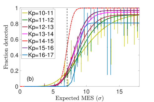
Figure 8: As for Figure 3, but calculated for different ranges in stellar magnitude.

4.3 CCD Channel

Another variable to consider is the location of the target in the Kepler field of view. There are a number of CCD channels which have been identified as producing a higher number of spurious long-period TCEs due to image artifacts (Thompson et al., 2018). Section 6.7 of Van Cleve et al. (2009) has additional information on the source of the artifacts. Here we examine whether target location influences the detection efficiency—in particular whether the over-abundance of long-period false positives on certain CCD channels reduces the detection efficiency of additional signals injected in the same light curve.

Since the field of view rotates every $\sim$90 days, a given group of targets (called a ‘sky group’) will fall on four distinct CCD channels over the course of a year, symmetrically positioned around the centre of the field of view. The number of the sky group and the number of the CCD channel upon which it falls are the same in Season 2, one of the four orientations of the spacecraft around the center of the field of view.

First we examine how the CDPP_L value varies across the field, since Section 4.2 establishes the dependence of the detection efficiency on this value. The upper panel of Figure 9 shows the median CDPP_L value across the field of view. The large black squares in the corners are the Fine Guidance Sensor CCDs, which were not used in the planet search. There are several notable features in the distribution of the median CDPP_L value. First, there is an underlying trend for increasing (worsening) CDPP_L values from the lower left to the upper right, which is correlated with decreasing Galactic latitude. With the relatively large Kepler pixels (4^′′/pixel), crowding becomes an increasing problem closer to the Galactic plane. This can increase the correlated noise measured across the CCD channel due to the increased likelihood of additional light from, e.g. background variable stars and eclipsing binaries. Four of the five channels with the highest (worst) CDPP_L values are visited by the sky groups that fall on CCD channel 58 during one of the four observing orientations. Channel 58 is one of the channels most strongly affected by the image artifacts described earlier, which is manifested here in the way the median CDPP_L value captures the correlated noise across the channel.

In the lower panel of Figure 9 we show the distribution of the plateau values ($c$ from Equation 1) across the field of view, for transit durations shorter than 15 hours, CDPP${}_{\rm L}<0$, and at least four transits. By restricting the injections to those shown previously to have the highest detection efficiency, we can examine any remaining influence of the CCD channels on the detection efficiency. There is a weak correlation in Figure 9 between the plateau value and the ring of best focus around the center of the focal plane (see Fig. 17 of Van Cleve & Caldwell, 2009)—9 out of 10 channels with the lowest detection efficiencies ($<$95%) are in the outer ring of modules (a module being a set of four CCD channels under the same field flattening lens), including the worst-performing channel 11. The CCDs with the best focus fall in a symmetric ring with a radius of $\sim 2--3^{\circ}$ around the center of the focal plane (the diameter of the full focal plane is $10^{\circ}$). Therefore, any targets that fall on these CCDs will experience less contamination from nearby targets—contamination which could introduce correlated noise and reduce the detection efficiency. We also examined the intra-CCD variation in the plateau values; the standard deviation varies from 0.11 to 0.23, with the same dependence across the field of view as in the upper panel of Figure 9.

We have labelled some of the sky groups which fall on known problematic channels for at least one orientation of the spacecraft during the year. Channels 44, 58, and 62 show the largest numbers of spurious TCEs caused by image artifacts, however the sky groups that fall on these channels do not show significantly decreased detection efficiency compared to the remainder of the channels. We conclude that the detection efficiency is not degraded in these channels with many spurious long-period TCEs, which is discussed further below.

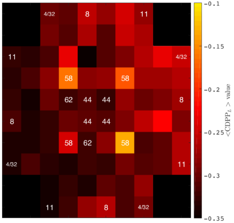
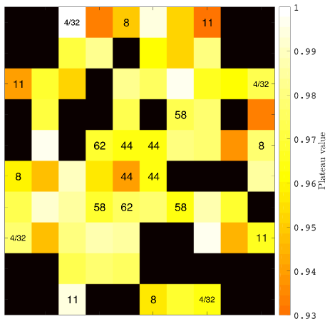
Figure 9: Upper: The median CDPP_L value value for each sky group. A clear trend across the field of view is evident, tracing the Galactic latitude and worsening with higher crowding at lower Galactic latitudes. One particularly poorly performing set of sky groups which fall on CCD channel 58 during the year are labelled. Lower: The detection efficiency plateau $c$ as a function of sky group for typically well-behaved targets. Nine out of ten of the worst performing channels are in the outer ring of modules; see text for additional detail.

5 Discussion

The results presented here examine, extend, and quantify the previous indications that there are various parameters which influence the detection efficiency of the Kepler pipeline. For occurrence rate calculations, this implies that with careful target selection, one could increase the completeness (lower the false negative rate) of a planet candidate catalog. The reliability of such a catalog would need to be re-calculated, which is beyond the scope of this paper. For the parameters examined here, we find that most of the detection efficiency differences (stellar temperature, stellar magnitude, position on the field of view) can be captured by the dependence on the correlated noise in the light curve as summarized by CDPP_L. Therefore, one can construct a target sample with a high and well-characterized completeness by removing 37,804 targets with positive CDPP_L values from the 198,709 targets searched to produced the final DR25 catalog.

One surprise was the similarity of the detection efficiency for CCDs with known correlated noise issues caused by image artifacts and of those without. As noted in Thompson et al. (2018), CCDs strongly affected by image artifacts produce a large over-abundance of weakly detected threshold crossing events with periods 300-500 days. A previous finding by Zink & Hansen (2019) had noted that the presence of multiple signals in the same light curve could degrade the detection efficiency. Therefore, it seemed likely that transit signals injected into targets on these CCDs may suffer reduced detection efficiency. However on closer investigation we find that this is not the case. The TPS module of the Kepler pipeline searches over a grid of period, epoch, and transit duration, and finds the combination which produces the strongest detection as measured by the Multiple Event Statistic (MES). For a light curve with multiple transiting signals, this will typically be the signal with the shortest orbital period. If this signal passes a series of vetoes, it is then removed from the light curve, which is then iteratively re-searched for additional signals which pass the MES detection threshold. This excision of data reduces the effective window function of the remaining data, and also affects the behavior of the harmonic fitter which removes sinusoidal trends in the light curve. Both of these have the effect of decreasing the detection efficiency for additional signals in the light curve.

For this experiment, injected signals were generated uniformly in period between 0.5–500 days. The majority of these signals therefore have shorter periods than the spurious signals generated by the image artifacts, and therefore their detection efficiency seems to be largely unaffected by those longer period image artifact signals, as the injected signals are detected first and removed. Analysing the longer period ($>400$ days) injections separately, we still see similar detection efficiency between the channels strongly affected by image artifacts and those that are not. Therefore, the impact of removing long period image artifact signals on the detection efficiency of additional long period signals in the light curve seems minimal, due to the fact that removal of long period image artifact signals from the light curve removes many fewer observation points than removal of shorter period signals, creating a much smaller reduction in the subsequent window function.

However, independent of the location on the field of view, we do show that the most complete planet candidate catalog is that which is confined to signals with periods $<350$ days. None of which is to say that one should not or cannot perform occurrence rate calculations for targets or signals outside of the bounds enumerated in this work, but that one would have to calculate and apply the appropriate completeness correction for the desired sample. For the target, sample defined above, with CDPP${}_{\rm L}<0$, the detection efficiency for injections with four or more transits, with injected transit durations shorter than 15 hours, and with orbital periods shorter than 350 days, is shown in Figure 10. The final best fit using Equation 1 is $\alpha=33.54$, $\beta=0.2478$, and a plateau of $c=97.31$%.

As discussed in Section 3, due to limitations on available resources the transit injection experiments were performed orthogonally—the wide-and-shallow pixel-level transit injections, with one injected signal per target, and the narrow-and-deep flux-level transit injections, with many thousands of signals injected into a smaller number of targets. A limitation of the pixel-level transit injections described in this work is that it averages over any fine structure in the response of the detection efficiency to features of the targets or the instrument, and provides only a description of the ensemble behavior. The flux-level transit injections were crucial, for instance, in identifying the role of the CDPP slope in discriminating between well- and poorly-behaved targets. However due to the relatively small number of targets probed by the flux-level transit injections, there may remain parameters to which the detection efficiency of the Kepler pipeline is sensitive that we have not yet identified. All of the light curves with simulated signals from the pixel- and flux-level transit injection experiments are available at the NASA Exoplanet Archive for further scrutiny by the community.

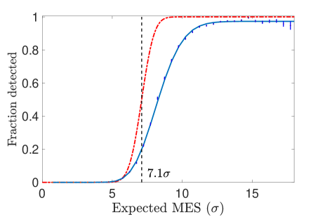
Figure 10: As for Figure 3, but calculated for the set of stars with CDPP${}_{\rm L}\leq 0$, for injected signals with four or more transits, orbital periods $<350$ days, and transit durations $<15$ hours.

6 Conclusions

This concludes the final Kepler project analysis of the detection efficiency of the Kepler pipeline. The performance of the SOC version 9.3 pipeline (Twicken et al., 2016) in producing the Data Release 25 planet candidate catalog (Thompson et al., 2018) was found to be a return to high detection efficiency after a moderate decrease in SOC version 9.2 (Christiansen et al., 2016). The dependence of the detection efficiency on the properties of both the targets and instrument were explored in some detail—the pipeline was found to have the highest detection efficiency for FGK stars ($4000\leq T_{\rm eff}\leq 7000$ K) with well-behaved noise properties. CCD channels with poor focus were found to have decreased detection efficiency, as were signals with periods longer than 300 days.

The fact that the response of the Kepler pipeline varied so strongly in different target and instrument parameter space speaks to the importance of transit injection experiments like the work described here. Analogous studies using data from missions like K2 and TESS, which have the opportunity to extend the occurrence rate results of Kepler beyond main sequence FGK stars, will similarly need to quantify the completeness and reliability of their resulting planet candidate catalogs to facilitate the generation of robust occurrence rates.

1. Not have an ephemeris which matches that of a previously identified TCE in any light curve, including the light curve being analysed;

2. Not have a secondary eclipse inconsistent with a planetary origin;

3. Not have statistically significant depth changes between the odd-numbered events and the even-numbered events (indicating an eclipsing binary system);

4. Not have a significantly v-shaped folded transit signal (also indicating an eclipsing binary system);

5. Have consistent depths for all measured transits (such that the folded signal strength is not dominated by one deeper event);

6. Be unique and statistically significant when compared to the correlated noise properties of the light curve when folded at the period of the TCE; and

7. Comprise at least three transits that have all individually passed a battery of additional tests interrogating their shape, coverage, and whether they fall during times which produce an inordinately high number of (likely spurious) signals.

Criteria 1 (identifying ephemeris matches) eliminates $\sim$0.05% of injected planets, Criteria 2–5 (identifying stellar eclipses) eliminate $\sim$1.3% of injected planets, and Criteria 6–7 (identifying non-transit-like events) eliminate $\sim$12% of injected planets; see Thompson et al. (2018) for additional details.

In the final mission-supported run of the Robovetter, the algorithms were tuned to maximise the reliability of the catalog for a given minimum completeness of shallow signals at long periods. This necessarily resulted in a sacrifice in the completeness of the catalog, or the number of the true positives promoted by the Robovetter. The goal of the transit injection and recovery experiment described in this work is to quantify the fraction of true positives that are lost as a result of this fine tuning. In DR25, the final run of the Robovetter resulted in 8,054 TCEs being classified as Kepler Objects of Interest (KOIs), and 4,034 of those as planet candidates (PCs).

References

- Akeson et al. (2013) Akeson, R. L., Chen, X., Ciardi, D., et al. 2013, PASP, 125, 989
- Berger et al. (2018) Berger, T. A., Huber, D., Gaidos, E., & van Saders, J. L. 2018, ApJ, 866, 99
- Brown et al. (2011) Brown, T. M., Latham, D. W., Everett, M. E., & Esquerdo, G. A. 2011, AJ, 142, 112
- Burke & Catanzarite (2017a) Burke, C. J., & Catanzarite, J. 2017a, NASA Exoplanet Archive, KSCI-19111-002
- Burke & Catanzarite (2017b) —. 2017b, NASA Exoplanet Archive, KSCI-19109-002
- Burke & Catanzarite (2017c) —. 2017c, Planet Detection Metrics: Window and One-Sigma Depth Functions for Data Release 25, Tech. rep.
- Christiansen (2017) Christiansen, J. L. 2017, NASA Exoplanet Archive, KSCI-19110-001
- Christiansen et al. (2012) Christiansen, J. L., Jenkins, J. M., Caldwell, D. A., et al. 2012, PASP, 124, 1279
- Christiansen et al. (2013) Christiansen, J. L., Clarke, B. D., Burke, C. J., et al. 2013, Astrophysical Journal Supplement, 207, 35
- Christiansen et al. (2015) —. 2015, Astrophysical Journal, 810, 95
- Christiansen et al. (2016) —. 2016, Astrophysical Journal, 828, 99
- Clarke et al. (2017) Clarke, B. D., Caldwell, D. A., Quintana, E. V., et al. 2017, Kepler Data Processing Handbook: Pixel Level Calibrations, Tech. rep.
- Coughlin (2017) Coughlin, J. L. 2017, Planet Detection Metrics: Robovetter Completeness and Effectiveness for Data Release 25 (KSCI-19114-002)
- Coughlin et al. (2016) Coughlin, J. L., Mullally, F., Thompson, S. E., et al. 2016, The Astrophysical Journal Supplement Series, 224, 12
- Jenkins (2017) Jenkins, J. M. 2017, Kepler Data Processing Handbook: Philosophy and Scope, Tech. rep.
- Jenkins et al. (1996) Jenkins, J. M., Doyle, L. R., & Cullers, D. K. 1996, Icarus, 119, 244
- Jenkins et al. (2017) Jenkins, J. M., Tenenbaum, P., Seader, S., et al. 2017, Kepler Data Processing Handbook: Transiting Planet Search, Tech. rep.
- Jenkins et al. (2010a) Jenkins, J. M., Chandrasekaran, H., McCauliff, S. D., et al. 2010a, Society of Photo-Optical Instrumentation Engineers (SPIE) Conference Series, Vol. 7740, Transiting planet search in the Kepler pipeline, 77400D
- Jenkins et al. (2010b) Jenkins, J. M., Chandrasekaran, H., McCauliff, S. D., et al. 2010b, in Society of Photo-Optical Instrumentation Engineers (SPIE) Conference Series, Vol. 7740, Proc. SPIE, 77400D
- Li et al. (2019) Li, J., Tenenbaum, P., Twicken, J. D., et al. 2019, PASP, 131, 024506
- Mandel & Agol (2002) Mandel, K., & Agol, E. 2002, ApJ, 580, L171
- Mathur et al. (2017) Mathur, S., Huber, D., Batalha, N. M., et al. 2017, ApJS, 229, 30
- Morris et al. (2017) Morris, R. L., Twicken, J. D., Smith, J. C., et al. 2017, Kepler Data Processing Handbook: Photometric Analysis, Tech. rep.
- Mullally et al. (2015) Mullally, F., Coughlin, J. L., Thompson, S. E., et al. 2015, ApJS, 217, 31
- Rowe et al. (2015) Rowe, J. F., Coughlin, J. L., Antoci, V., et al. 2015, ApJS, 217, 16
- Smith et al. (2017a) Smith, J. C., Morris, R. L., Jenkins, J. M., et al. 2017a, Kepler Data Processing Handbook: Finding Optimal Apertures in Kepler Data, Tech. rep.
- Smith et al. (2012) Smith, J. C., Stumpe, M. C., Van Cleve, J. E., et al. 2012, PASP, 124, 1000
- Smith et al. (2017b) Smith, J. C., Stumpe, M. C., Jenkins, J. M., et al. 2017b, Kepler Data Processing Handbook: Presearch Data Conditioning, Tech. rep.
- Thompson et al. (2018) Thompson, S. E., Coughlin, J. L., Hoffman, K., et al. 2018, Astrophysical Journal Supplement, 235, 38
- Twicken et al. (2016) Twicken, J. D., Jenkins, J. M., Seader, S. E., et al. 2016, Astrophysical Journal, 152, 158
- Twicken et al. (2018) Twicken, J. D., Catanzarite, J. H., Clarke, B. D., et al. 2018, PASP, 130, 064502
- Van Cleve & Caldwell (2009) Van Cleve, J. E., & Caldwell, D. A. 2009, MAST Archive, KSCI-19033-001
- Van Cleve et al. (2009) Van Cleve, J. E., Christiansen, J. L., Jenkins, J. M., et al. 2009, MAST Archive, KSCI-19040-005
- Zink & Hansen (2019) Zink, J. K., & Hansen, B. M. S. 2019, MNRAS, 487, 246