Reparametrizing gradient descent

Abstract. In this work, we propose an optimization algorithm which we call norm-adapted gradient descent. This algorithm is similar to other gradient-based optimization algorithms like Adam or Adagrad in that it adapts the learning rate of stochastic gradient descent at each iteration. However, rather than using statistical properties of observed gradients, norm-adapted gradient descent relies on a first-order estimate of the effect of a standard gradient descent update step, much like the Newton-Raphson method in many dimensions. Our algorithm can also be compared to quasi-Newton methods, but we seek roots rather than stationary points. Seeking roots can be justified by the fact that for models with sufficient capacity measured by nonnegative loss functions, roots coincide with global optima. This work presents several experiments where we have used our algorithm; in these results, it appears norm-adapted descent is particularly strong in regression settings but is also capable of training classifiers.

1 Introduction

We propose an optimization algorithm closely related to gradient descent. In short, to find the minimizing input of a nonnegative real-valued function $f$, our proposal replaces the standard gradient update step

$$\theta_{i+1}\leftarrow\theta_{i}-\eta\cdot\nabla_{\theta}f({\theta_{i}})$$ (1)

with a new step

$$\theta_{i+1}\leftarrow\theta_{i}-\alpha\cdot\frac{f(\theta_{i})}{\left\lVert\nabla_{\theta}f({\theta_{i}})\right\rVert^{2}}\nabla_{\theta}f({\theta_{i}})$$ (2)

We call the resulting algorithm “norm-adapted gradient descent” and call gradient descent with the update step (1) “standard gradient descent” for purposes of disambiguation. This paper gives reasons for this modification, analyzes some strengths and weaknesses of this proposal, and presents some experimental evidence on its performance.

Input: $f:\mathbb{R}^{k}\to[L,\infty)$ a differentiable function, $L\in\mathbb{R}$ a lower bound on the output of $f$ (usually $L=0$), $\theta_{0}\in\mathbb{R}^{k}$ an initial guess, $\alpha\in[0,2]$ a percent decrease target

Output: $\theta_{N}\in\mathbb{R}^{k}$, an input value making $f(\theta_{N})\approx L$

1 $i\leftarrow 0$

2 while progress_insufficient() do

       $\theta_{i+1}\leftarrow\theta_{i}-\min(1,\alpha\cdot\frac{f(\theta_{i})-L}{\left\lVert\nabla_{\theta}f({\theta_{i}})\right\rVert^{2}})\cdot\nabla_{\theta}f({\theta_{i}})$

        // update step (2)

3       $i\leftarrow i+1$

4      

5 end while

return $\theta_{i}$

Algorithm 1 Norm-adapted gradient descent

One way to describe norm-adapted gradient descent is that it performs a variant of the Newton-Raphson root-finding algorithm. Recall in the case $f:\mathbb{R}\to\mathbb{R}$, the Newton-Raphson method approximates $f(\theta)$ as the first-order function $f(\theta_{i})+(\theta-\theta_{i})\cdot f^{\prime}(\theta_{i})$ around $\theta_{i}$ and then chooses $\theta_{i+1}\leftarrow\theta_{i}-\frac{f(\theta_{i})}{f^{\prime}(\theta_{i})}$, the value of $\theta$ that would make this approximation 0.

In the case $f:\mathbb{R}^{n}\to[0,\infty)$, we first restrict our search for a root from $\theta_{i}$ to the $-\nabla_{\theta}f({\theta_{i}})$ direction. The appropriate Newton-Raphson update is then $\theta_{i+1}\leftarrow\theta_{i}-\frac{f(\theta_{i})}{\left\lVert\nabla_{\theta}f({\theta_{i}})\right\rVert}\cdot\frac{\nabla_{\theta}f({\theta_{i}})}{\left\lVert\nabla_{\theta}f({\theta_{i}})\right\rVert}$. We introduce a hyperparameter $\alpha$, analogous to the learning rate in standard gradient descent, after which we have the update step (2) above.

To see that (2) is the appropriate Newton-Raphson update, consider the first-order approximation of the effect of the update step (1) on the value of $f$. From the fact that $\frac{\partial}{\partial\eta}f(\theta_{i}+\eta\cdot\nabla_{\theta}f({\theta_{i}}))=\left\lVert\nabla_{\theta}f({\theta_{i}})\right\rVert^{2}$,

$$f(\theta_{i}-\eta\cdot\nabla_{\theta}f({\theta_{i}}))=f(\theta_{i})-\eta\cdot\left\lVert\nabla_{\theta}f({\theta_{i}})\right\rVert^{2}+o(\eta^{2}).$$ (3)

The update step (2) chooses the learning rate $\eta\mathbin{\triangleq}\alpha\cdot\frac{f(\theta_{i})}{\left\lVert\nabla_{\theta}f({\theta_{i}})\right\rVert^{2}}$ which reduces the right hand side of the approximation (3) to $(1-\alpha)f(\theta_{i})$ plus the error term.

This lends a natural interpretation to norm-adapted gradient descent: it adjusts the learning rate at every step to attempt to reduce the value of the target function by a fixed fraction $\alpha$. This in turn suggests $\alpha$ should be drawn from $[0,1]$. (In practice, we have found values of $\alpha$ up to 2 can be useful.) This is one reason for the title of this paper—norm-adapted descent is similar to stochastic gradient descent but with a different hyperparameter which has a different interpretation.

When the gradient has a small norm, the update step (2) has some numerical instability, so we bound the scalar coefficient of the gradient with a maximum value of 1, as seen on line 3 in Algorithm 1. The threshold value of 1 was chosen since learning rates are never, to our knowledge, chosen outside [0, 1] and this factor can be seen as the equivalent of a learning rate in standard gradient descent.

Norm-adapted gradient descent is a root-finding algorithm. When using it in a machine learning context we are taking advantage of the fact that most error functions take nonnegative values. In models with sufficient capacity, the true global minimum value will be close to zero, and this coincidence between optimum values and roots allows us to use root-finding algorithms. When optimizing functions which have some known non-zero lower bound $L$, the numerator of the update in (2) can be modified to $f(\theta_{i})-L$. Further adaptation is required for situations where the global minimum value is not known in advance; this is one situation where $\alpha>1$ can be useful.

The numerator $f(\theta_{i})$ in (2) provides a measure of global progress to the minimum value, making the algorithm take bigger steps when the current function value is large. Since norm-adapted gradient descent has access to this global information, it is better able to distinguish local minima from global minima and behaves rather differently from ordinary gradient descent near local minima and saddle points.

Another important property of norm-adapted descent is its invariance to scaling of the target function—it treats $f(\theta)$ and $k\cdot f(\theta)$ exactly the same. Steps taken by standard gradient descent for the latter are scaled by a factor of $k$ compared to the former, and the optimal learning rates will differ by a factor of $k$ as well. We have found that norm-adapted descent generally requires less hyperparameter tuning and suspect this property may be part of the reason why.

2 Simple functions

In this section, we examine the performance of these gradient descent optimizers on some simple functions. For now, we restrict our attention to gradient descent and our norm-adapted variant. As we progress to more practical benchmarks, we will consider other common optimizers like Adam.

We consider two functions: $q(x,y)\mathbin{\triangleq}8x^{2}+\frac{1}{2}y^{2}$ and $r(x,y)\mathbin{\triangleq}(1-x)^{2}+100(y-x^{2})^{2}$, the Rosenbrock function. These both present “valley problems” to gradient-based algorithms, which typically make rapid progress moving down the slope of the valley but struggle along the valley floor. The “valleys” for these functions are the $y$-axis for the quadratic function and a parabolic valley along $y=x^{2}$ for the Rosenbrock function. The global minimum for each of these functions is 0, located at (0, 0) for $q$ and at $(1,1)$ for $r$.

2.1 Results summaries

Table 1 presents data about the performance of standard gradient descent (SGD) and norm-adapted gradient descent (NaSGD) optimizers when attempting to find points such that $q(x,y)\leq 10^{-10}$ starting from the initial point $(1,1)$. We give three kinds of instances for each algorithm: first the best hyperparameter value we could find, then results with more typical hyperparameter values that one might try first, and finally average results from 2000 trials with hyperparameter values uniformly sampled from an interval.

	Steps to reach:					Time (& scaled to best SGD run):
	$10^{-2}$	$10^{-4}$	$10^{-6}$	$10^{-8}$	$10^{-10}$	ms/run		$\mu$s/step
SGD($\eta=0.1156$)	23	39	56	74	92	18.2	(1)	198	(1)
NaSGD($\alpha=1.9$)	4	6	10	13	15	4.8	(0.27)	322	(1.63)
SGD($\eta=0.0100$)	196	425	654	883	1113	233.5	(12.79)	210	(1.06)
SGD($\eta=0.1000$)	20	42	64	86	107	21.2	(1.16)	198	(1.00)
NaSGD($\alpha=0.7$)	12	22	32	42	53	16.2	(0.89)	306	(1.54)
NaSGD($\alpha\sim[0.2,2]$)	13.5	23.35	33.18	43.03	52.8	15.9	(0.87)	300	(1.51)

Table 1: Steps and time to achieve $q(x_{i},y_{i})\leq 10^{-10}$ from $(x_{0},y_{0})=(1,1)$

In this scenario, though a step of norm-adapted descent takes 50-65% longer than a step of standard gradient descent, a large reduction in the number of steps required leads to an overall decrease in the time required to reach the target threshold by 10-70%. The absolute times reported here were obtained on a 2017 MacBook Pro, 2.3 GHz i5, with 16GB RAM.

Table 2 gives similar data for optimizing the Rosenbrock function $r$ starting from $(-3,-4)$. In this table, entries marked $\uparrow$ indicate the algorithm diverged (meaning parameter values became large).

	Steps to reach:					Time (& scaled to best SGD run):
	$10^{2}$	$10^{0}$	$10^{-2}$	$10^{-4}$	$10^{-6}$	ms/run		$\mu$s/step
SGD($\eta=0.0003945$)	7	9	14	20	13633	3956.4	(1)	290	(1)
NaSGD($\alpha=1.6$)	5	10	57	166	236	84.4	(0.02)	358	(1.23)
SGD($\eta=0.0001$)	66	254	31683	85861	142986	37806.6	(9.56)	264	(0.91)
SGD($\eta=0.0010$)	$\uparrow$	$\uparrow$	$\uparrow$	$\uparrow$	$\uparrow$	—	(—)	—	(—)
NaSGD($\alpha=0.7$)	9	16	147	354	497	185.9	(0.05)	374	(1.29)
NaSGD($\alpha\sim[0.2,2]$)	8.37	14.89	152.2	390.31	641.93	239.7	(0.06)	373	(1.29)

Table 2: Steps and time to achieve $r(x_{i},y_{i})\leq 10^{-6}$ from $(x_{0},y_{0})=(-3,-4)$

The results here are broadly similar to the quadratic function: individual steps of norm-adapted descent are more costly than those of standard gradient descent, but the overall time to reach the lower values is considerably reduced since fewer steps are required. The per-step overhead involved in norm-adapted descent is the cost to compute the squared norm of the gradient, since all the other quantities are computed in standard gradient descent.

Hyperparameter tuning for norm-adapted descent is relatively easy: choosing a random $\alpha\in[0.2,2]$ yields, on average, performance competitive with the best version of standard gradient descent we could find in both scenarios. In contrast, learning rates for gradient descent are sensitive to the scale of the function, and no learning rate works out-of-the-box in both cases. Learning rates in the $10^{-3}$ or $10^{-4}$ range are intolerably slow for the quadratic function, while learning rates in the $10^{-1}$ or $10^{-2}$ range for the Rosenbrock function cause immediate divergence. The Rosenbrock function, a common test function in optimization, is particularly tricky: gradient descent seems to start diverging with learning rates higher than $0.0003948$, while our best-performing learning rate is just barely under this value.

2.2 Vector fields

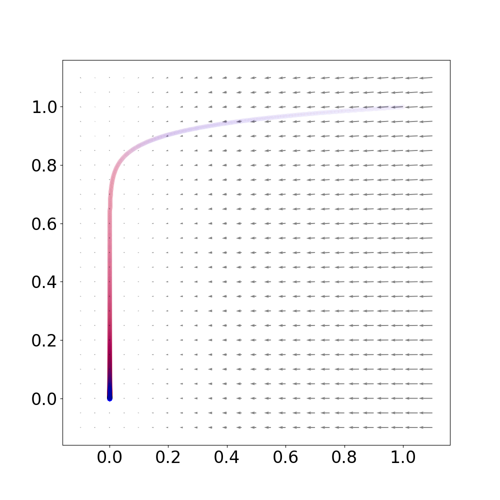
Figure 1: Comparing limit behavior

We can get some insight into why these two algorithms perform the way they do by considering what they do in the limit. In figure 1, we have plotted the vector field $\vec{x}\mapsto-\nabla q(\vec{x})$, together with two series of very light circles. In light blue circles are the first 6000 values NaSGD($\alpha=0.007$) goes through while optimizing $q$ from $(1,1)$. In light red are the first 6000 values SGD($\eta=0.001$) visits while optimizing the same function from the same point.

The fact that there is a single curve from $(1,1)$ to $(0,0)$ indicates that in the limit (as $\alpha,\eta\to 0$), these two algorithms transit through the same points. The fact that this curve is not a uniform color also contains important information. Where the curve is darker, at least one of the algorithms is spending more time: norm-adapted descent is spending more time in the bluer regions, and standard gradient descent spends more time in redder regions.

We can illustrate this further by plotting the points each algorithm visits when these hyperparameters are multiplied by 10 (Figure 2). As we can see, norm-adapted descent takes much smaller steps initially, taking much longer to reach an $x$-value under 0.2. However, as the two processes begin moving mostly in the $y$-direction, norm-adapted descent picks up speed: individual points are distinguishable whereas in standard gradient descent they are not.

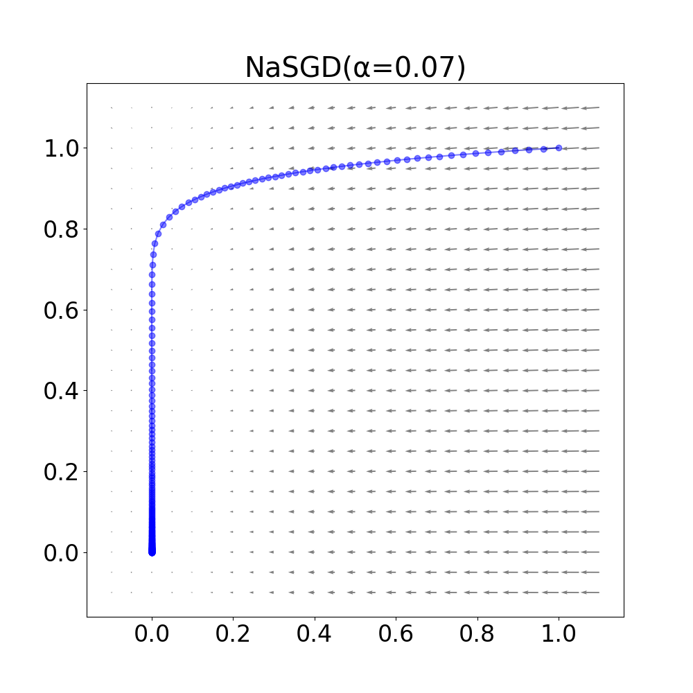
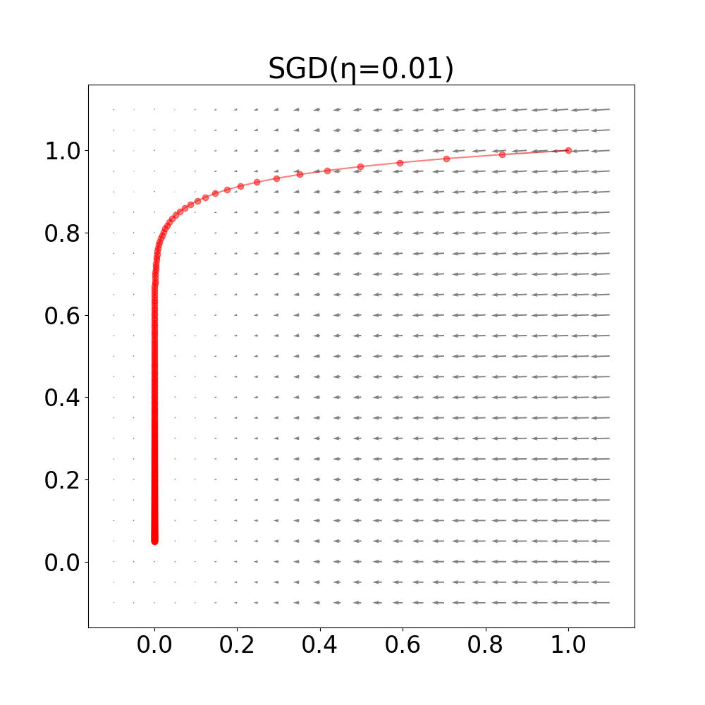
Figure 2: Points visited by norm-adapted descent and gradient descent

There is a nice reason for these phenomena. Both types of gradient descent are finding approximations to integral flows for two vector fields which have the same direction at every point ($\vec{x}\mapsto-\nabla q(\vec{x})$ for standard gradient descent and $\vec{x}\mapsto-\frac{q(\vec{x})}{\left\lVert q(\vec{x})\right\rVert^{2}}\nabla q(\vec{x})$ for norm-adapted descent), but which may have different lengths. The fact that these vector fields have the same direction everywhere means their integral flows pass through the same set of points, and the fact that these fields usually have different lengths mean the two integral flows pass through those points at different speeds. This is the second justification for our title—the two versions of gradient descent effectively transit the same curve, but with different parameterizations in time.

In particular, since standard gradient descent follows the gradient vector field, it moves quickly through regions where the gradient has a large norm and slowly through regions where the norm is small. This is why standard gradient descent makes more rapid progress in the $x$-direction while optimizing $q$—the gradient of $q$ along the $y$-axis is comparatively small. Norm-adapted descent behaves differently. The length of its vector field at $\vec{x}$ is $\frac{q(\vec{x})}{\left\lVert q(\vec{x}))\right\rVert}$, so larger gradients slow down norm-adapted descent and small gradients accelerate it. This is the reason it is able to transit the “valley floor” along the $y$-axis quickly.

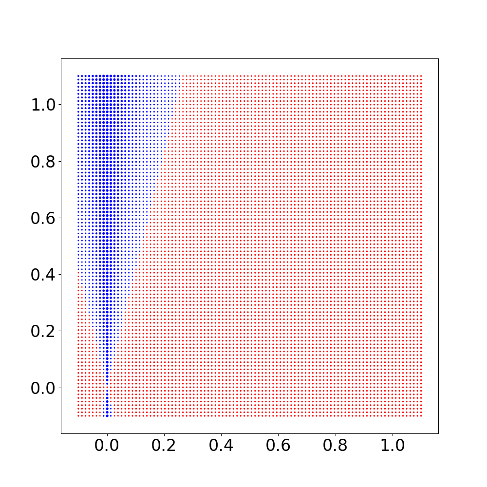
Figure 3: Speed advantages

The net effect of all of this is that norm-adapted descent moves more slowly in regions where standard gradient descent moves quickly and conversely. While this might seem to be a balanced trade, it is decidedly to norm-adapted descent’s advantage: decreasing the difference between the speeds in the two regions considerably raises their harmonic mean.

Figure 3 depicts the ratio between the lengths of the two vector fields at each point in space. We plot a red circle at points where standard gradient descent is following a longer vector and conversely a blue circle where norm-adapted descent is longer. The area of the circle is proportional to the ratio of the larger to the smaller. We also include a factor of the ratio of the optimal learning rates, since the magnitudes of the learning rates affect the speed of the convergence.

Standard gradient descent has a consistent advantage away from the $y$-axis, following a gradient field which is moving about twice as fast. Closer to the $y$-axis, norm-adapted descent acquires a large advantage, following a gradient field which is about eight times larger than standard gradient descent.

3 Dense layer matching task

In this section, we continue our examination of norm-adapted gradient descent in increasingly applied contexts. Here we will look at a somewhat contrived machine learning task: a layer recovery. In this task, we randomly initialized a dense layer $\mathbb{R}^{10}\to\mathbb{R}^{4}$ with a $\tanh$ activation function. We then randomly sampled 200 input points from $[0,1]^{10}$ and ran the dense layer on these points to get corresponding outputs. We split this artificial dataset into two equally sized subsets, one for training and one for testing.

We randomly initialized layers of the same shape and trained them on the test set in an attempt to recover the original layer. We measured progress on this task as the average distance between the expected and predicted values on the test set. We used various optimizers to train each network for 45 passes through the data with minibatches of size 1. Therefore, in the graphs below, 100 training steps correspond to an epoch of training. We repeated this experiment 50 times and report on the averages achieved in these 50 runs.

This scenario is unusually well-suited for neural networks; it is much more typical to have no guarantees about how well the data-generating process under consideration can modeled by our network architecture. Here, we know that our model has the exact right amount of capacity and is structured in the best possible way. The primary challenge here is using a relatively limited amount of data to recover the parameters. However, common optimization algorithms struggle to achieve average distances lower than $10^{-3}$ between the actual and expected points.

3.1 Results summaries

In figure 4, we plot the base-10 logarithm of the average distance between actual test values and the values produced by the networks trained by standard gradient descent with various learning rates as a function of the number of training steps. Each plot corresponds to a different value of momentum, indicated in the title of the plot as $\mu$; each series corresponds to a different learning rate, indicated in the legend as $\eta$.

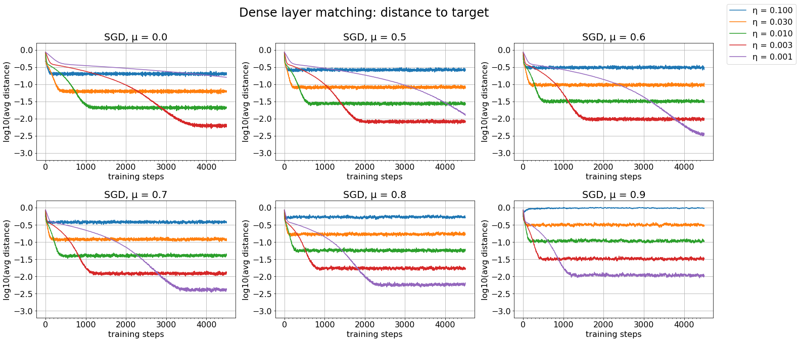
Figure 4: Standard gradient descent with momentum in the dense layer matching task

As we can see, each learning rate seems to have a saturation point beyond which further training does not improve performance. Higher learning rates reach their saturation points quicker, while lower learning rates saturate at better performance levels. Raising the value the momentum parameter causes overall gains in speeds of convergence but carries some cost in terms of final performance, findings consistent with [8].

Other common optimization algorithms (Adam, RMSprop, and Adagrad) similarly struggle to break $10^{-3}$, as shown in figure 5. Norm-adapted descent achieves average distances lower than $10^{-3}$ with progress stabilizing around $10^{-7}$ for $\alpha\in[0.5,1.5]$. Norm-adapted descent with $\alpha\in[0.1,0.3]$ is competitive with standard algorithms, and $\alpha\geq 1.7$ appears not to make progress.

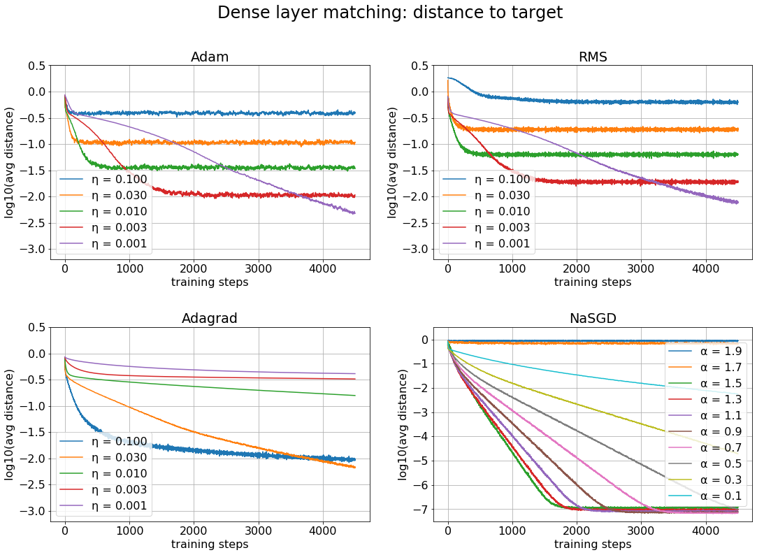
Figure 5: Adam, RMSprop, Adagrad, and NaSGD in the dense layer matching task

3.2 Translating between hyperparameters

A useful coincidence between standard gradient descent and our norm-adapted variant is the fact that they follow the same direction field. This means that for each step taken by standard gradient descent we can calculate the equivalent $\alpha$ which would produce the exact same step when used in norm-adapted descent, and conversely we can calculate the equivalent $\eta$ for each step taken by norm-adapted descent. We present the average such equivalent parameters over the 50 runs in the first two plots in figure 6 below.

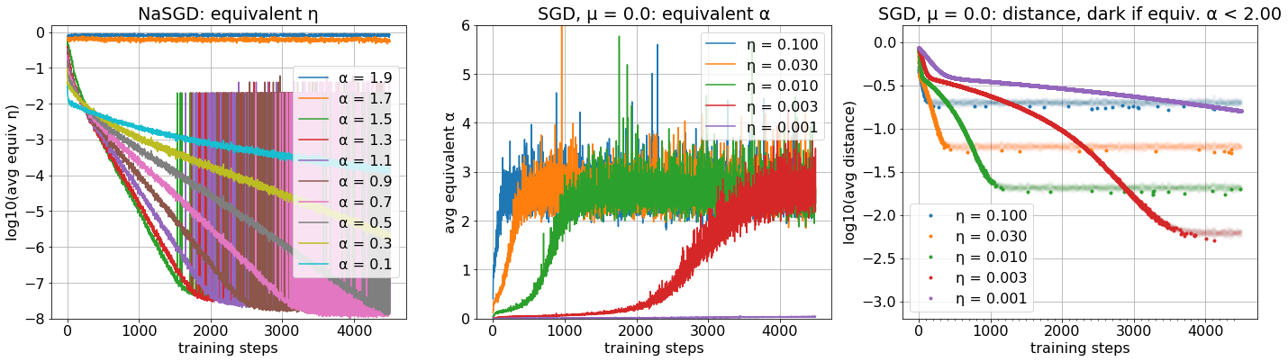
Figure 6: Rosetta stone: equivalent hyperparameters for other algorithm

As we see in the first plot, though norm-adapted descent could end up having equivalent learning rates anywhere in the $[0,1]$ interval at any time, it generally decreases the learning rate from 1 to $10^{-8}$ as its performance improves. One way to interpret this is that it is performing an adaptive learning rate scheduling based on the current loss value and gradient.

The second plot shows standard gradient descent starts with low equivalent $\alpha$, which tends to increase during the course of training, settling above 2. This means that the steps taken by standard gradient descent should result in a 200-300% decrease in loss according to the estimate (3). This is obviously overambitious; loss can decrease by at most 100% for nonnegative functions.

Though we have observed $\alpha\in[0,2]$ can be performant for norm-adapted descent, rarely has $\alpha>2$ resulted in good performance. Thus, this “equivalent $\alpha$” statistic may be a good indicator for a high learning rate in gradient descent. In the third plot of figure 6, we show the same accuracy series as in the first plot in figure 4, but fade the points if the equivalent $\alpha$ in that step is greater than 2. The result suggests a general rule: gradient descent makes progress in this task when the equivalent $\alpha$ value is below 2 and stops making progress when its equivalent $\alpha$ value is above 2.

The diagnostic role of this translation works in the other direction too: norm-adapted descent makes steady progress while its equivalent learning rate decreases steadily. After converging, the equivalent learning rate seems to oscillate in magnitude quite significantly. This information could possibly used to design a stopping tactic for norm-adapted descent.

3.3 The utility of the Newton-Raphson estimate

There is a natural question at this point about the fundamental reason for the performance differences between gradient descent and the norm-adapted variant. The equivalent $\eta$ graph in figure 6 suggests norm-adapted descent has an exponentially decreasing learning rate, and scheduling a learning rate to follow such a function is a known technique which often improves performance at the cost of tuning further hyperparameters (namely the base of the exponential decay). So, is adapting the learning rate using the Newton-Raphson estimate actually important to the performance of norm-adapted descent, or is it basically a mimicking mechanism for learning rate scheduling?

To address this question, we consider two different kinds of optimizers. In the first class, we fit an exponential to the average equivalent learning rate of norm-adapted descent ($\alpha=0.7$) in this task and use this exponential as the learning rate schedule for an otherwise standard gradient descent. In the second class, we do a standard gradient descent while monitoring its equivalent $\alpha$ value. If that $\alpha$ value exceeds some threshhold too often, we decrease the learning rate. If norm-adapted descent gets its performance by somehow choosing a good schedule, we would expect the first class to behave similarly on average to NaSGD($\alpha=0.7$). If the Newton-Raphson estimate provides a useful signal for reducing learning rate adaptively, we would expect the second class to do well.

In the end, the first class, imitating norm-adapted descent’s average equivalent learning rate, does not perform particularly well in this task. We tried fitting three different exponentials—one for the best fit in the first 1500 (series labeled “decay028”), first 600 (“decay052”) and first 200 steps (“decay090”) each. However, none performed particularly well.

We only tried one member of the second class (“alpha100”), where we multiplied the learning rate (starting at $\eta=0.1$) by $\frac{1}{3}$ each time $\alpha\geq 2.0$ happened for 3 consecutive steps. This simplistic policy has somewhat comparable performance to NaSGD($\alpha=0.7$) (“gna070”), and achieves an average distance of $10^{-3}$ from the expected values, which is better than the standard optimizers described above. In the plots of figure 7, we show the average accuracies and average learning rates (or equivalent learning rates) of these five algorithms in the first 1500 steps (15 epochs) of the same 50 runs as used in the experiments above.

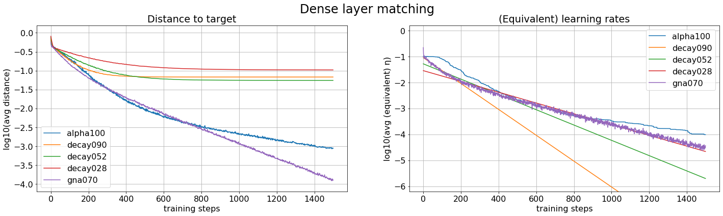
Figure 7: Exponential decay scheduling vs equivalent $\alpha$ monitoring

As a result, we believe that the Newton-Raphson modeling of the function and norm-adapted descent’s continuous monitoring of this quantity plays a critical role in its enhanced performance.

4 MNIST

Finally, we consider a standard problem in machine learning: classification on the MNIST dataset [6]. We train simple convolutional neural networks to classify these images, with two convolutional layers (5x5 filters with 10 then 20 features) with 2x2 max pooling layers after each convolution and ending with two dense layers with 50 then 10 output neurons. For regularization, we included dropout on the second convolution and first dense layers and normalized the pixel value distribution. This is a relatively small convolutional network, but with enough capacity to regularly classify 97% of MNIST images correctly.

A one-hot encoding of the correct class is used as the target value in $\mathbb{R}^{10}$, and we use a cross-entropy loss function. We train the network in minibatches of size 60 so an epoch consists of 1000 minibatches. We completed 20 different runs consisting of 200 epochs with many different optimizers and learning rates. The data presented in table 3 and figure 8 are averages of these 20 runs for selected high-performance learning rates for each optimizer.

Our findings largely fit with the results of Kingma and Ba [5], though our model is less complex. Adam shows clear performance benefits over RMSprop and Adagrad in both accuracy and loss. They consider SGD with Nesterov momentum, while we present SGD with ordinary momentum, so those series are less comparable. While SGD performs best in this task, norm-adapted gradient descent is certainly competitive with SGD and Adam and achieves an edge over RMSprop and Adagrad.

Optimizer name	Accuracy (higher better)		Optimizer name	Loss (lower better)
SGD($\eta$ = 0.001, $\mu$ = 0.9)	0.9751		SGD($\eta$ = 0.03, $\mu$ = 0.0)	0.0705
SGD($\eta$ = 0.03, $\mu$ = 0.0)	0.9747		Adam($\eta$ = 0.001)	0.0726
NaSGD($\alpha$ = 0.5)	0.9745		SGD($\eta$ = 0.001, $\mu$ = 0.9)	0.0752
Adam($\eta$ = 0.001)	0.9729		NaSGD($\alpha$ = 0.5)	0.0783
RMSprop($\eta$ = 0.001)	0.9698		RMSprop($\eta$ = 0.001)	0.0938
Adagrad($\eta$ = 0.01)	0.9696		Adagrad($\eta$ = 0.01)	0.103

Table 3: MNIST: selected optimizers sorted by two performance metrics after 200 epochs of training

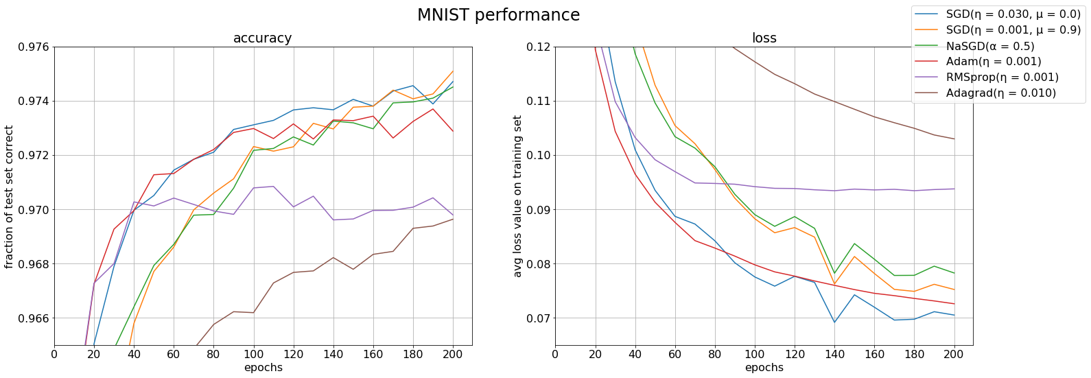
Figure 8: MNIST: performance metrics plotted

5 Related work

Norm-adapted gradient descent is a gradient-based optimization algorithm used for training neural networks and is naturally related to other works which propose algorithms in this same class. Adam [5], Adagrad [4], RMSprop [9], Adadelta [10], gradient descent with momentum and Nesterov updates [3, 8] are some examples of these kinds of algorithms, commonly used and available in many deep learning frameworks.

Each of these optimization algorithms modify SGD using statistical properties of the gradients seen in the training process, such as weighted means of past gradients (SGD with momentum), raw second moments (Adagrad, RMSprop, and Adadelta), or both (Adam). Norm-adapted descent relies on the estimate of an update’s effect (3) and uses no such historical data, making it a largely orthogonal development. This presents exciting opportunities for further research: what is a sensible Newton-Raphson update step for these other algorithms and how does it perform?

Another related family of algorithms are quasi-Newton methods, such as BFGS. A common use of the Newton-Raphson method for root-finding is to search for roots of the derivative of a function—such points include all optima of differentiable functions. The update scheme for this version of Newton’s method is $\theta_{i+1}\leftarrow\theta_{i}-[H_{f}(\theta_{i})]^{-1}\nabla_{\theta}f({\theta_{i}})$, where the Jacobian is the function being zeroed so the Hessian matrix takes the role of derivative. Computing Hessians for high-dimensional functions is usually considered prohibitively expensive, so quasi-Newton methods maintain approximations to the Hessian.

Norm-adapted descent relies on a coincidence between optima and roots which allows us to do root-finding on the original function rather than its derivative. This saves some of the higher-order complications present in quasi-Newton methods at the expense of generality, namely the risk of failing to converge if the minimum value of the function is not known in advance. The nonnegativity of most loss functions in machine learning helps mitigate this weakness of NaSGD.

One advantage of norm-adapted descent over these other gradient-based algorithms, including quasi-Newton methods, is a resistance to saddle points and local minima. Incorporating the current value of the loss function allows norm-adapted descent to differentiate between global minima and stationary points: areas around both have small gradient vectors but only around the latter will also have greater loss values. This advantage comes with an obvious drawback: if the global minimum is not known in advance or is inaccurately approximated (e.g. when trying to fit a model with insufficent capacity), norm-adapted descent does not readily settle into a global minimum.

Norm-adapted descent can also be seen as a gradient-based algorithm which adjusts its learning rate at every step. Other works which adjust hyperparameters in the course of training include [7, 2]. The key difference between our work and these approaches is that our learning rate adjustment is made based on the Newton-Raphson estimate, rather than local curvature information or the gradient of a learning step with respect to a hyperparameter.

6 Conclusion and future directions

In this work, we have described a new algorithm for training neural networks, norm-adapted gradient descent, which is based on the Newton-Raphson method in many dimensions. We described several experiements demonstrating the practical performance of our algorithm. Norm-adapted gradient descent performs particularly well in regression tasks, posting order-of-magnitude improvements in performance over well-known optimizers. Norm-adapted descent also performed well in the MNIST classification task, certainly competitive with other well-known optimizers.

As noted above, norm-adapted descent breaks from the tradition of using statistical information about gradients observed in the training process and instead relies on the Newton-Raphson method to adapt the learning rate. The orthogonality of this development leads to some interesting questions: could similar adaptations be developed for SGD with momentum, Adam, etc?

We also noted the translatability between the learning rates in norm-adapted descent and stochastic gradient descent leads to some insights about the performance of both of these algorithms. We are interested in further exploiting these observations to develop hybrid optimization algorithms like those alluded to in section 3.3.

Finally, though norm-adapted descent shows great promise based on the experiments we were able to conduct, it will certainly be interesting to see its performance on more advanced tasks.

References

- [1] Proceedings of the 30th International Conference on Machine Learning, ICML 2013, Atlanta, GA, USA, 16-21 June 2013, volume 28 of JMLR Workshop and Conference Proceedings. JMLR.org, 2013.
- [2] Kartik Chandra, Erik Meijer, Samantha Andow, Emilio Arroyo-Fang, Irene Dea, Johann George, Melissa Grueter, Basil Hosmer, Steffi Stumpos, Alanna Tempest, and et al. Gradient descent: The ultimate optimizer. arXiv:1909.13371 [cs, stat], Sep 2019. arXiv: 1909.13371.
- [3] Timothy Dozat. Incorporating Nesterov momentum into Adam. 2016.
- [4] John C. Duchi, Elad Hazan, and Yoram Singer. Adaptive subgradient methods for online learning and stochastic optimization. J. Mach. Learn. Res., 12:2121–2159, 2011.
- [5] Diederik P. Kingma and Jimmy Ba. Adam: A method for stochastic optimization. In Yoshua Bengio and Yann LeCun, editors, 3rd International Conference on Learning Representations, ICLR 2015, San Diego, CA, USA, May 7-9, 2015, Conference Track Proceedings, 2015.
- [6] Yann LeCun and Corinna Cortes. MNIST handwritten digit database. 2010.
- [7] Tom Schaul, Sixin Zhang, and Yann LeCun. No more pesky learning rates. In Proceedings of the 30th International Conference on Machine Learning, ICML 2013, Atlanta, GA, USA, 16-21 June 2013 [1], pages 343–351.
- [8] Ilya Sutskever, James Martens, George E. Dahl, and Geoffrey E. Hinton. On the importance of initialization and momentum in deep learning. In Proceedings of the 30th International Conference on Machine Learning, ICML 2013, Atlanta, GA, USA, 16-21 June 2013 [1], pages 1139–1147.
- [9] T. Tieleman and G. Hinton. Lecture 6.5—RmsProp: Divide the gradient by a running average of its recent magnitude. COURSERA: Neural Networks for Machine Learning, 2012.
- [10] Matthew D. Zeiler. ADADELTA: an adaptive learning rate method. CoRR, abs/1212.5701, 2012.