On the similarity between ranking vectors in the pairwise comparison method

Abstract

There are many priority deriving methods for pairwise comparison matrices. It is known that when these matrices are consistent all these methods result in the same priority vector. However, when they are inconsistent, the results may vary. The presented work formulates an estimation of the difference between priority vectors in the two most popular ranking methods: the eigenvalue method and the geometric mean method. The estimation provided refers to the inconsistency of the pairwise comparison matrix. Theoretical considerations are accompanied by Montecarlo experiments showing the discrepancy between the values of both methods.

1 Introduction

Creating a ranking based on comparing alternatives in pairs was already known in the Middle Ages. Probably the first work on this subject was by Ramon Llull [6], who described election procedures based on the mutual comparisons of alternatives. Over time, more and more studies on the pairwise comparison method emerged. It is necessary to mention here works on electoral systems, such as the Condorcet method [7] and the Copeland method [31], and many studies on the social choice and welfare systems [35]. At the beginning of the twentieth century, alternatives began to be compared quantitatively. This was initially associated with the need to compare psychophysical stimuli [11, 36, 37]. It was later developed [10] and used in various forms for different purposes, including economics [28], consumer research [12], psychometrics [30], health care [19, 29] and others. Thanks to Saaty and his seminal work in which he defined AHP (Analytic Hierarchy Process) [32], comparing alternatives in pairs began to be seen primarily as a multi-criteria decision-making method. The incredible success of AHP is partly due to the fact that Saaty proposed a complete ready-to-use solution including a ranking calculation algorithm, an inconsistency index as a method of determining data quality, and a hierarchical model allowing users to handle multiple criteria. However, it turned out quite quickly [9, 1] that the proposed solutions can be improved. The research conducted on the pairwise comparison method has resulted in many priority deriving algorithms [18, 16] and inconsistency indices [3, 25, 24]. Probably the two most popular algorithms for calculating priorities are EVM (Eigenvalue method proposed by Saaty) and GMM (Geometric mean method devised by Crawford) [32, 8]. It is easy to verify that, for a consistent matrix, both methods lead to the same solution. In the case of inconsistent matrices, the resulting rankings differ from each other. Herman and Koczkodaj have proved experimentally that the more consistent the matrices are, the more similar the rankings [17]. The presented article complements their Montecarlo evidence with the analytical proof of this convergence. It also shows the results of a new Montecarlo experiment. Thanks to this, the reader receives a method that enables estimation of how far apart the results of both of the most popular ranking methods can be: EVM and GMM. The presented work is part of the discussion on the properties of the pairwise comparison method and AHP. Despite the large number of publications on this topic [4, 27, 22, 2], the AHP method continues to inspire and challenge researchers.

The article is composed of five sections. The current introductory section precedes Preliminaries, which includes basic concepts and definitions. The third section is entirely devoted to theoretical considerations. It contains theorems showing the relationships between ranking vectors calculated using the EVM and GMM methods with reference to the inconsistency of the PC matrix. The next section shows the result of the Montecarlo experiments carried out. A brief summary and discussions can be found in the last section of the article.

2 Preliminaries

When making choices, people make comparisons. When paying for an apple in a store, we choose the larger one, putting products on the scale, we compare their weight with the standard of one kilogram, etc. Comparing alternatives in pairs allows us to create a ranking and choose the best possible option. In AHP as proposed by Saaty [32] all alternatives are compared to each other. Hence, the ranking data creates the matrix in which rows and columns correspond to alternatives and individual elements represent the results of comparisons. Such matrices are the subjects of priority deriving methods, which transform them into weight vectors. The i-th component of such a vector corresponds to the importance of the i-th alternative. The credibility of such a ranking depends on the consistency of the set of comparisons. It has been accepted that the more consistent the set of comparisons is, the more reliably the assessment is made. Below, we will briefly introduce basic methods for calculating priorities and estimating inconsistency for matrices containing the results of pairwise comparisons of alternatives.

2.1 PC matrices and priority deriving methods

The input data for the priority deriving method is a PC (pairwise comparison) matrix $C=[c_{ij}]$ of non-negative elements. The values of $c_{ij}$ and $c_{ji}$ indicate the relative importance (or preference) of the i-th and j-th alternatives. We denote alternatives using the lowercase letter $a$ together with an appropriate integer index. The set of all alternatives is given as $A=\{a_{1},\ldots,a_{n}\}$. Because comparing an alternative with itself ends up in a tie, then the diagonal of the matrix is filled up with ones. Formally, the PC matrix can be defined as follows.

Definition 1.

The PC matrix of the order $n$ is an $n\times n$ square matrix $\mathbf{C}=[c_{ij}]$ given as follows:

$$\mathbf{C}=\left[\begin{array}[]{cccc}1&c_{12}&...&c_{1n}\\ c_{21}&1&...&...\\ ...&...&1&...\\ c_{n1}&...&...&1\end{array}\right],$$

where $c_{ij}\in\mathbb{R}_{+}$.

Definition 2.

The matrix $\mathbf{C}=[c_{ij}]$ is said to be (multiplicatively) reciprocal if:

$$\forall i,j\in\{1,\ldots,n\}:c_{ij}\cdot c_{ji}=1.$$ (1)

There are two main methods allowing us to calculate the priority vector (vector of weights)

$$w=\left[w(a_{1}),\ldots,w(a_{n})\right]^{T}$$

from the PC matrix $\mathbf{C}=[c_{ij}]$. There is the eigenvalue method (EVM) proposed by Saaty [32], and the geometric mean method (GMM) proposed by Crawford [8].

In EVM, the priority vector is an eigenvector corresponding to the largest eigenvalue of $\mathbf{C}$:

$$\mathbf{C}\mathbf{w}_{\textit{max}}=\lambda_{\textit{max}}\mathbf{w}_{\textit{max}},$$ (2)

where $\lambda_{max}\geq n$ is a positive eigenvalue, and $\mathbf{w}_{\textit{max}}$ is the corresponding (right) eigenvector of $\mathbf{C}$. The priority vector $w$ is given as $w=\gamma\cdot\mathbf{w}_{max}$, where $\gamma$ is a scaling factor, $\gamma=\left(\sum_{i=1}^{n}w_{\textit{max}}(a_{i})\right)^{-1}$, so that $\|w\|_{m}=1$.

In GMM, which is, in principle, equivalent to the logarithmic least squares method [8], the priority vector $\mathbf{w}$ is derived as the geometric mean of all rows of $\mathbf{C}$:

$$w=\gamma\left[\left(\prod_{r=1}^{n}c_{1r}\right)^{\frac{1}{n}},\ldots,\left(\prod_{r=1}^{n}c_{nr}\right)^{\frac{1}{n}}\right]^{T}$$ (3)

where $\gamma$ is a scaling factor so that $\|w\|=1$.

Example 3.

Let us consider the following PC matrix

$$\mathbf{C}=\left[\begin{array}[]{cccc}1&\frac{1}{2}&2&5\\ 2&1&4&4\\ \frac{1}{2}&\frac{1}{4}&1&5\\ \frac{1}{5}&\frac{1}{4}&\frac{1}{5}&1\end{array}\right],$$

Using the methods defined above, it is easy to verify that the priority vectors $\mathbf{w_{\textit{EV}}}$ and $\mathbf{w_{\textit{GM}}}$ of $\mathbf{C}$ are $\mathbf{w_{\textit{EV}}}=\left[0.282,0.474,0.179,0.065\right]^{T}$, $\mathbf{w_{\textit{GM}}}=\left[0.294,0.468,0.175,0.062\right]^{T}$.

In addition to these two main methods of calculating priorities, there are a number of other solutions. A good starting point for further literature research are the works [5, 14].

2.2 Inconsistency

When comparing both alternatives, experts try to ensure that the value obtained corresponds exactly to the ratio between the real priority of both alternatives, i.e.

$$c_{ij}=\frac{w(a_{i})}{w(a_{j})}.$$ (4)

Hence, it is natural to expect that

$$c_{ij}=\frac{w(a_{i})}{w(a_{j})}=\frac{w(a_{i})}{w(a_{k})}\cdot\frac{w(a_{k})}{w(a_{j})}=c_{ik}c_{kj}.$$

If this is not the case, the set of comparisons is inconsistent.

Definition 4.

The PC matrix $\mathbf{C}=[c_{ij}]$ is said to be (multiplicatively) consistent if:

$$\forall i,j,k\in\{1,\ldots,n\}:c_{ij}\cdot c_{jk}\cdot c_{ki}=1.$$ (5)

It is easy to observe that each consistent PC matrix corresponds exactly to one weight vector and, reversely, the weight vector induces exactly one consistent PC matrix.

Definition 5.

Let $w$ be the ranking vector

$$w=\left(\begin{array}[]{c}w(a_{1})\\ \vdots\\ \vdots\\ w(a_{n})\end{array}\right).$$

The consistent PC matrix $C$ induced by $w$ is given as

$$C=\left(\begin{array}[]{cccc}\frac{w(a_{1})}{w(a_{1})}&\frac{w(a_{1})}{w(a_{2})}&\cdots&\frac{w(a_{1})}{w(a_{n})}\\ \frac{w(a_{2})}{w(a_{1})}&\ddots&\cdots&\vdots\\ \vdots&\cdots&\ddots&\vdots\\ \frac{w(a_{n})}{w(a_{1})}&\cdots&\cdots&\frac{w(a_{n})}{w(a_{n})}\end{array}\right).$$

It is easy to prove that all ranking procedures following the principle (4) produce identical priority vectors for consistent PC matrices.

It is accepted that the level of inconsistency is measured by inconsistency indices. The first inconsistency index for the PC matrix CI was proposed by Saaty [32].

Definition 6.

The inconsistency index CI of a PC matrix $\mathbf{C}$ of the order $n$ is defined as follows

$$\textit{CI}(\mathbf{C})=\frac{\lambda_{max}-n}{n-1},$$ (6)

The value $\lambda_{\textit{max}}\geq n$, and $\lambda_{\textit{max}}=n$ only if a pairwise comparison matrix is consistent [33]. Thus, when $\mathbf{C}$ is consistent then $\textit{CI}(\mathbf{C})=0$. Defining the inconsistency index resulted in a question about the limits above which the index reaches unacceptable values. Answering this question, Saaty proposed consideration of the inconsistency of a PC matrix as acceptable providing that it is ten times lower than the CI of a totally random matrix of the same size. To link the inconsistency index CI with random matrices, the concept of the consistency ratio CR was introduced.

Definition 7.

The consistency ratio CR is defined as

$$\textit{CR}(\mathbf{C})=\frac{\textit{CI}(\mathbf{C})}{\textit{RI}(n)},$$ (7)

where $\textit{RI}(n)$ denotes the random consistency index dependent on $n$.

Following the above definition, the inconsistency of $\mathbf{C}$ is considered as acceptable if $\textit{CR}(\mathbf{C})\leq 0.1$.

Another inconsistency index comes from Koczkodaj [21]. However, while $\textit{CI}(\mathbf{C})$ measures some average inconsistency in $\mathbf{C}$, Koczkodaj’s index focuses on the inconsistencies of individual triads $c_{ik},c_{kj},c_{ij}$ (see Def. 4). Following the popular saying of “one rotten apple spoils the barrel” it finds the maximum local inconsistency (9) and accepts it as the inconsistency of the entire matrix.

Definition 8.

Koczkodaj’s inconsistency index KI of an $n\times n$ and ($n>2)$ reciprocal matrix $\mathbf{C}=[c_{ij}]$ is defined as follows: [21]

$$\textit{KI}_{i,k,j}=\min\left\{\left|1-\frac{c_{ij}}{c_{ik}c_{kj}}\right|,\left|1-\frac{c_{ik}c_{kj}}{c_{ij}}\right|\right\}$$ (8)

$$\textit{KI}(C)=\underset{i,j,k\in\{1,\ldots,n\}}{\max}\textit{KI}_{i,k,j}$$ (9)

Remark 9.

It is easy to observe that $0\leq KI(\mathbf{C}=[c_{ij}])<1$.

More information about various inconsistency indices can be found in [3, 24].

2.3 Comparing ranking data

2.3.1 Comparing ranking vectors

In the era of increasing use of rankings, the ability to compare them is a must. Music charts, the ten best films of the year, and academic rankings of world universities (Shanghai list) are just a few examples of the rankings we have to deal with on a daily basis. One of the first methods for comparing rankings comes from Kendall [26, 20]. This is an ordinal index of similarity indicating the number of necessary transpositions of consecutive alternatives needed to transform one ranking into another. We may also treat cardinal rankings as vectors in $n$ dimensional space. Thus, the difference between ranking vectors can be estimated using Manhattan distance:

$$\textit{MD}(w_{1},w_{2})\overset{\textit{df}}{=}\sum_{i=1}^{n}\left|w_{1}(a_{i})-w_{2}(a_{i})\right|$$ (10)

[26] or Tchebyshev distance

$$\textit{ChD}(w_{1},w_{2})\overset{\textit{df}}{=}\left\|w_{1}-w_{2}\right\|_{\infty}=\max_{i=1,\ldots,n}\left|w_{1}(a_{i})-w_{2}(a_{i})\right|$$

see [15, p. 845]. However, working with rankings based on comparisons of alternatives in pairs and knowing their nature (4), we decided to propose another indicator of their similarity (defined in Subsection 3.1).

2.3.2 Comparing PC matrices

When two experts evaluate the same set of alternatives, one may expect that the results of their assessments are similar. This similarity can be assessed by comparing PC matrices. For this purpose, we can use the compatibility index defined by Saaty [34].

Definition 10.

Let $C_{1}=[c_{ij}^{(1)}],C_{2}=[c_{ij}^{(2)}]$ be the reciprocal PC matrices of the same size $n\times n$. The compatibility index of $C_{1}$ and $C_{2}$ is given as

$$\textit{comp}(C_{1},C_{2})\overset{\textit{df}}{=}\frac{1}{n^{2}}e^{T}C_{1}\circ C_{2}^{T}e=\frac{1}{n^{2}}\sum_{i=1}^{n}\sum_{j=1}^{n}c_{ij}^{(1)}\cdot c_{ji}^{(2)},$$

where $e^{T}=[1,\ldots,1]$.

This index is the sum of the individual entries creating the Hadamard product of reciprocal matrices $C_{1}=[c_{ij}]$ and $C_{2}^{T}=[c_{ji}]$ divided by their number. Hence, its value is a kind of arithmetic average of expressions in the form $c_{ij}^{(1)}\cdot c_{ji}^{(2)}$. It is easy to observe that $\textit{comp}(C_{1},C_{2})$ for two identical values returns $1.$ When the matrices are different, this value increases.

3 How far apart are EVM and GMM?

The concept of matrix compatibility (Def. 10) can easily be extended to ranking vectors. Thanks to this, we gain an additional way to compare two ranking vectors. Later on in this section, we will show the relationship between inconsistency measured by Koczkodaj’s Index (Def. 8) and the compatibility of ranking vectors. It will also be shown that this reasoning can be extended to classic vector distance measures, such as Manhattan distance (10).

However, before we define the compatibility index for priority vectors, let us extend the compatibility index for matrices. One of the disadvantages of the compatibility index (Def. 10) is that each pair $c_{ij}^{(1)}\cdot c_{ji}^{(2)}$ is compared two times. The first time directly, the second time as its reverse $c_{ji}^{(1)}\cdot c_{ij}^{(2)}$. Another inconvenience is the fact that pairs in the form $c_{ii}^{(1)}\cdot c_{ii}^{(2)}$ always equal $1$, hence such pairs contribute nothing to our knowledge of the compatibility level. The last problem stems from the fact that the compatibility index is a summation of ratios in the form $x/y$. Thus, one may expect that every component $x/y$ contributes the same as $y/x$ to the value of the index. Of course, that is not the case as the greater $x$ is compared to $y$ the more important the component $x/y$ becomes and $y/x$ becomes less important. The solution may be to choose the larger element from each pair in the form $\left\{c_{ij}^{(1)}\cdot c_{ji}^{(2)},c_{ji}^{(1)}\cdot c_{ij}^{(2)}\right\}$ and limit the summation to the upper triangles of both matrices. The above considerations allow us to formulate an improved definition of the vector compatibility index. In order to distinguish it from the original version, we will denote it as $\overline{\textit{comp}}$.

Definition 11.

Let $C_{1}=[c_{ij}^{(1)}],C_{2}=[c_{ij}^{(2)}]$ be the reciprocal PC matrices of the same size $n\times n$. The upper compatibility index of $C_{1}$ and $C_{2}$ is given as

$$\overline{\textit{comp}}(C_{1},C_{2})\overset{\textit{df}}{=}\frac{2}{n(n-1)}\sum_{\begin{subarray}{c}i,j=1\\ j>i\end{subarray}}^{n}\max\left\{c_{ij}^{(1)}\cdot c_{ji}^{(2)},c_{ji}^{(1)}\cdot c_{ij}^{(2)}\right\}$$ (11)

Of course, replacing the maximum by minimum would also be justified. I.e.

Definition 12.

Let $C_{1}=[c_{ij}^{(1)}],C_{2}=[c_{ij}^{(2)}]$ be the reciprocal PC matrices of the same size $n\times n$. The lower compatibility index of $C_{1}$ and $C_{2}$ is given as

$$\underline{\textit{comp}}(C_{1},C_{2})\overset{\textit{df}}{=}\frac{2}{n(n-1)}\sum_{\begin{subarray}{c}i,j=1\\ j>i\end{subarray}}^{n}\min\left\{c_{ij}^{(1)}\cdot c_{ji}^{(2)},c_{ji}^{(1)}\cdot c_{ij}^{(2)}\right\}$$ (12)

The only difference between $\overline{\textit{comp}}$ and $\underline{\textit{comp}}$ is that in the case of $\overline{\textit{comp}}$ higher values of the index mean higher total incompatibility, while in the case of $\underline{comp}$ the opposite is true. Lower values of $\underline{\textit{comp}}$ mean higher total incompatibility of the compared matrices. In both cases, matrices $C_{1}$ and $C_{2}$ that are fully compatible will result in $\overline{\textit{comp}}(C_{1},C_{2})=\underline{\textit{comp}}(C_{1},C_{2})=1$.

Sometimes, it can also be useful to determine the maximum local incompatibility of two PC matrices. In order to determine this value, let us introduce the last modification of the original compatibility index.

Definition 13.

Let $C_{1}=[c_{ij}^{(1)}],C_{2}=[c_{ij}^{(2)}]$ be the reciprocal PC matrices of the same size $n\times n$. The maximal compatibility index of $C_{1}$ and $C_{2}$ is given as

$$\textit{compmax}(C_{1},C_{2})\overset{\textit{df}}{=}\underset{i,j=1,\ldots,n}{\max}c_{ij}^{(1)}\cdot c_{ji}^{(2)}$$ (13)

Remark 14.

It is easy to prove that for two PC matrices $C_{1}$ and $C_{2}$ it holds that

$$\underline{\textit{comp}}(C_{1},C_{2})\leq\textit{comp}(C_{1},C_{2})\leq\overline{\textit{comp}}(C_{1},C_{2})\leq\textit{compmax}(C_{1},C_{2}).$$

3.1 Compatibility of ranking vectors

Armed with a number of compatibility indices for matrices, we can easily extend their definitions to ranking vectors.

Definition 15.

Let $w_{1}$ and $w_{2}$ be the ranking vectors, and $C_{1}$ and $C_{2}$ be the PC matrices induced by $w_{1}$ and $w_{2}$ (see Def. 5). The compatibility indices of $w_{1}$ and $w_{2}$, written as $\textit{comp}(w_{1},w_{2})$, $\overline{\textit{comp}}(w_{1},w_{2})$, $\underline{\textit{comp}}(w_{1},w_{2})$ and $\textit{compmax}(w_{1},w_{2})$ are defined as $\textit{comp}(C_{1},C_{2})$, $\overline{\textit{comp}}(C_{1},C_{2})$, $\underline{\textit{comp}}(C_{1},C_{2})$ and $\textit{compmax}(C_{1},C_{2})$ correspondingly.

Remark 16.

Providing that $w_{1}=[w_{1}(a_{1}),\ldots,w_{1}(a_{n})]^{T}$ and $w_{2}=[w_{2}(a_{1}),\ldots,w_{2}(a_{n})]^{T}$ and

$$\beta_{ij}(w_{1},w_{2})\overset{\textit{df}}{=}\frac{w_{1}(a_{i})}{w_{1}(a_{j})}\cdot\frac{w_{2}(a_{j})}{w_{2}(a_{i})},$$

the vector compatibility indices can be written as

$$\textit{comp}(w_{1},w_{2})\overset{\textit{df}}{=}\frac{1}{n^{2}}\sum_{i,j=1}^{n}\beta_{ij}(w_{1},w_{2}),$$ (14)

$$\overline{\textit{comp}}(w_{1},w_{2})\overset{\textit{df}}{=}\frac{2}{n(n-1)}\sum_{\begin{subarray}{c}i=1,j=2\\ j>i\end{subarray}}^{n}\max\left\{\beta_{ij}(w_{1},w_{2}),\beta_{ji}(w_{1},w_{2})\right\},$$ (15)

$$\textit{$\underline{comp}$}(w_{1},w_{2})\overset{\textit{df}}{=}\frac{2}{n(n-1)}\sum_{\begin{subarray}{c}i=1,j=2\\ j>i\end{subarray}}^{n}\min\left\{\beta_{ij}(w_{1},w_{2}),\beta_{ji}(w_{1},w_{2})\right\}$$ (16)

and

$$\textit{compmax}(w_{1},w_{2})\overset{\textit{df}}{=}\underset{i,j=1,\ldots,n}{\max}\beta_{ij}(w_{1},w_{2})$$

Theorem 17.

For every $n\times n$ PC matrix $C$ the compatibility indices of two rankings $w_{\textit{ev}}$ and $w_{\textit{gm}}$ where the first is computed using EVM and the latter using GMM satisfy the following inequalities:

$$\kappa^{2} \leq\underline{\textit{comp}}(w_{\textit{ev}},w_{\textit{gm}})\leq\textit{comp}(w_{\textit{ev}},w_{\textit{gm}})\leq$$ (17)

$$\leq\overline{\textit{comp}}(w_{\textit{ev}},w_{\textit{gm}})\leq\textit{compmax}(w_{\textit{ev}},w_{\textit{gm}})\leq\frac{1}{\kappa^{2}},$$

where $\kappa=1-\textit{KI}(C)$.

Proof.

Based on the definition of KI we obtain

$$\textit{KI}(C)\geq\min\left\{\left|1-\frac{c_{ij}}{c_{ik}c_{kj}}\right|,\left|1-\frac{c_{ik}c_{kj}}{c_{ij}}\right|\right\}$$ (18)

This means that either:

$$c_{ij}\leq c_{ik}c_{kj}\,\,\text{implies}\,\,\textit{KI}(C)\geq 1-\frac{c_{ij}}{c_{ik}c_{kj}}$$ (19)

or

$$c_{ik}c_{kj}\leq c_{ij}\,\,\text{implies}\,\,\textit{KI}(C)\geq 1-\frac{c_{ik}c_{kj}}{c_{ij}}$$ (20)

is true. Let us denote $\kappa\overset{\textit{df}}{=}1-\mathscr{\textit{KI}}(C)$. The above can then be written as:

$$c_{ij}\leq c_{ik}c_{kj}\,\,\text{implies}\,\,c_{ij}\geq\alpha\cdot c_{ik}c_{kj}$$ (21)

$$c_{ik}c_{kj}\leq c_{ij}\,\,\text{implies}\,\,\frac{1}{\alpha}\cdot c_{ik}c_{kj}\geq c_{ij}$$ (22)

Since $\kappa\leq 1$ , both cases (21) and (22) lead independently to the common conclusion that:

$$\kappa\cdot c_{ik}c_{kj}\leq c_{ij}\leq\frac{1}{\kappa}c_{ik}c_{kj}$$ (23)

Due to the definition of GMM ranking, the ratio of the i-th and j-th elements of the priority vector $w_{\textit{gm}}$ equals

$$\frac{w_{\textit{gm}}(a_{j})}{w_{\textit{gm}}(a_{i})}=\frac{\left(\prod_{r=1}^{n}c_{jr}w_{\textit{gm}}(a_{r})\right)^{\frac{1}{n}}}{\left(\prod_{r=1}^{n}c_{ir}w_{\textit{gm}}(a_{r})\right)^{\frac{1}{n}}}.$$

Thus, based on (23) we obtain that

$$\frac{w_{\textit{gm}}(a_{j})}{w_{\textit{gm}}(a_{i})}\leq\frac{\left(\prod_{r=1}^{n}\frac{1}{\kappa}c_{ji}c_{ir}w_{\textit{gm}}(a_{r})\right)^{\frac{1}{n}}}{\left(\prod_{r=1}^{n}c_{ir}w_{\textit{gm}}(a_{r})\right)^{\frac{1}{n}}}=\frac{1}{\kappa}c_{ji}.$$

For the same purpose we obtain

$$\kappa c_{ji}=\frac{\left(\prod_{r=1}^{n}\kappa c_{ji}c_{ir}w_{\textit{gm}}(a_{r})\right)^{\frac{1}{n}}}{\left(\prod_{r=1}^{n}c_{ir}w_{\textit{gm}}(a_{r})\right)^{\frac{1}{n}}}\leq\frac{w_{\textit{gm}}(a_{j})}{w_{\textit{gm}}(a_{i})}.$$

In other words

$$\kappa c_{ji}\leq\frac{w_{\textit{gm}}(a_{j})}{w_{\textit{gm}}(a_{i})}\leq\frac{1}{\kappa}c_{ji}.$$ (24)

Similarly for EVM we have [23]:

$$\frac{w_{\textit{ev}}(a_{i})}{w_{\textit{ev}}(a_{j})}=\frac{\sum_{r=1}^{n}c_{ir}w_{\textit{ev}}(a_{r})}{\sum_{r=1}^{n}c_{jr}w_{\textit{ev}}(a_{r})}.$$

Hence, due to (23) we have

$$\frac{w_{\textit{ev}}(a_{i})}{w_{\textit{ev}}(a_{j})}\leq\frac{\sum_{r=1}^{n}\frac{1}{\kappa}c_{ij}c_{jr}w_{\textit{ev}}(a_{r})}{\sum_{r=1}^{n}c_{jr}w_{\textit{ev}}(a_{r})}=\frac{1}{\kappa}c_{ij}.$$

Once again, we can also obtain

$$\kappa c_{ij}=\frac{\sum_{r=1}^{n}\kappa c_{ij}c_{jr}w_{\textit{ev}}(a_{r})}{\sum_{r=1}^{n}c_{jr}w_{\textit{ev}}(a_{r})}\leq\frac{w_{\textit{ev}}(a_{i})}{w_{\textit{ev}}(a_{j})}.$$

Thus, we get

$$\kappa c_{ij}\leq\frac{w_{\textit{ev}}(a_{i})}{w_{\textit{ev}}(a_{j})}\leq\frac{1}{\kappa}c_{ij}.$$ (25)

By multiplying sidewise (24) and (25) we obtain

$$\kappa^{2}\leq\frac{w_{\textit{ev}}(a_{i})}{w_{\textit{ev}}(a_{j})}\cdot\frac{w_{\textit{gm}}(a_{j})}{w_{\textit{gm}}(a_{i})}\leq\frac{1}{\kappa^{2}},$$

i.e.

$$\kappa^{2}\leq\beta_{ij}(w_{\textit{ev}},w_{\textit{gm}})\leq\frac{1}{\kappa^{2}},$$ (26)

for any $i,j=1,\ldots,n$.

It is easy to observe that the above induces both

$$\kappa^{2}\leq\underline{\textit{comp}}(w_{\textit{ev}},w_{\textit{gm}}),$$

and

$$\textit{compmax}(w_{\textit{ev}},w_{\textit{gm}})\leq\frac{1}{\kappa^{2}}.$$

Thus, in the light of (Rem. 14) the thesis (17) of the theorem is satisfied. ∎

The above theorem shows that the compatibility of two ranking vectors can move within the range determined by the value of inconsistency. On the one hand, it cannot be smaller than $\kappa^{2}$. This means that, for example, if there is non-zero inconsistency both vectors cannot be fully compatible. In other words, as long as $C$ is inconsistent both vectors $w_{\textit{ev}}$ and $w_{\textit{gm}}$ cannot be identical. On the other hand, their compatibility indices cannot be greater than $\kappa^{-2}$. This means in particular that, for relatively small values of inconsistency, both ranking vectors are very similar.

3.2 Local compatibility and the distance between rankings

The result of Theorem 17 can be presented even more precisely. That is because the ranking vectors calculated using EVM and GMM are very often rescaled so that their components sum up to $1$. Let us write down this observation in the form of the following lemma.

Lemma 18.

For every $n\times n$ PC matrix $C$ and two rankings $w_{\textit{ev}}$ and $w_{\textit{gm}}$ where the first is computed using EVM and the latter using GMM and

$$\sum_{i=1}^{n}w_{\textit{ev}}(a_{i})=1,\,\,\,\,\sum_{i=1}^{n}w_{\textit{gm}}(a_{i})=1,$$

it holds that

$$\kappa^{2}\leq\frac{w_{\textit{ev}}(a_{i})}{w_{\textit{gm}}(a_{j})}\leq\frac{1}{\kappa^{2}},$$

for $i,j=1,.\ldots,n$, where $\kappa=1-\textit{KI}(C)$.

Proof.

According to (26) it holds that

$$\kappa^{2}\leq\frac{w_{\textit{ev}}(a_{i})}{w_{\textit{ev}}(a_{j})}\cdot\frac{w_{\textit{gm}}(a_{j})}{w_{\textit{gm}}(a_{i})}\leq\frac{1}{\kappa^{2}}.$$

Thus

$$w_{\textit{ev}}(a_{1})\kappa^{2}\leq\frac{w_{\textit{ev}}(a_{i})}{1}\cdot\frac{w_{\textit{gm}}(a_{1})}{w_{\textit{gm}}(a_{i})}\leq\frac{1}{\kappa^{2}}w_{\textit{ev}}(a_{1})$$

$$w_{\textit{ev}}(a_{2})\kappa^{2}\leq\frac{w_{\textit{ev}}(a_{i})}{1}\cdot\frac{w_{\textit{gm}}(a_{2})}{w_{\textit{gm}}(a_{i})}\leq\frac{1}{\kappa^{2}}w_{\textit{ev}}(a_{2})$$

$$\vdots$$

$$w_{\textit{ev}}(a_{n})\kappa^{2}\leq\frac{w_{\textit{ev}}(a_{i})}{1}\cdot\frac{w_{\textit{gm}}(a_{n})}{w_{\textit{gm}}(a_{i})}\leq\frac{1}{\kappa^{2}}w_{\textit{ev}}(a_{n})$$

By summing the above $n$ equalities on the left and right hand sides, we obtain

$$\kappa^{2}\sum_{j=1}^{n}w_{\textit{ev}}(a_{j})\leq\sum_{j=1}^{n}\frac{w_{\textit{ev}}(a_{i})}{1}\cdot\frac{w_{\textit{gm}}(a_{j})}{w_{\textit{gm}}(a_{i})}\leq\frac{1}{\kappa^{2}}\sum_{j=1}^{n}w_{\textit{ev}}(a_{j}),$$

hence

$$\kappa^{2}\sum_{j=1}^{n}w_{\textit{ev}}(a_{j})\leq\frac{w_{\textit{ev}}(a_{i})}{w_{\textit{gm}}(a_{i})}\sum_{j=1}^{n}w_{\textit{gm}}(a_{j})\leq\frac{1}{\kappa^{2}}\sum_{j=1}^{n}w_{\textit{ev}}(a_{j}).$$

Since $\sum_{j=1}^{n}w_{\textit{ev}}(a_{j})=\sum_{j=1}^{n}w_{\textit{gm}}(a_{j})=1$, then the above reduces to

$$\kappa^{2}\leq\frac{w_{\textit{ev}}(a_{i})}{w_{\textit{gm}}(a_{i})}\leq\frac{1}{\kappa^{2}}.$$

Of course, it also holds that

$$\kappa^{2}\leq\frac{w_{\textit{gm}}(a_{i})}{w_{\textit{ev}}(a_{i})}\leq\frac{1}{\kappa^{2}}.$$

∎

The above lemma allows us to estimate the Manhattan distance measure between the EVM and GMM ranking vectors using the inconsistency index KI.

Theorem 19.

For every $n\times n$ PC matrix $C$ and two rankings $w_{\textit{ev}}$ and $w_{\textit{gm}}$ where the first is computed using EVM and the latter using GMM and

$$\sum_{i=1}^{n}w_{\textit{ev}}(a_{i})=1,\,\,\,\,\sum_{i=1}^{n}w_{\textit{gm}}(a_{i})=1,$$

it holds that

$$n\left(\kappa^{2}-1\right)\leq\textit{MD}(w_{\textit{ev}},w_{\textit{gm}})\leq n\left(\frac{1}{\kappa^{2}}-1\right),$$ (27)

where $\kappa=1-\textit{KI}(C)$.

Proof.

Based on Lemma 18 we obtain

$$\kappa^{2}w_{\textit{gm}}(a_{i})\leq w_{\textit{ev}}(a_{i})\leq\frac{1}{\kappa^{2}}w_{\textit{gm}}(a_{i}).$$ (28)

We use the above inequality to determine the maximal distance between $w_{\textit{ev}}(a_{i})$ and $w_{\textit{gm}}(a_{i})$. Let us consider the value $d_{i}=\left|w_{\textit{ev}}(a_{i})-w_{\textit{gm}}(a_{i})\right|$ in terms of two cases: $w_{\textit{ev}}(a_{i})\leq w_{\textit{gm}}(a_{i})$ and $w_{\textit{ev}}(a_{i})\geq w_{\textit{gm}}(a_{i})$. If the first situation holds, the greater $d_{i}$ is, the smaller $w_{\textit{ev}}(a_{i})$. Hence, due to (28), an upper bound for $d_{i}$ is $w_{\textit{gm}}(a_{i})-\kappa^{2}w_{\textit{gm}}(a_{i})=w_{\textit{gm}}(a_{i})\left(1-\kappa^{2}\right)$. In the second case, the greater $d_{i}$ is, the higher $w_{\textit{ev}}(a_{i})$. Thus, an upper bound for $d_{i}$ is $\frac{1}{\kappa^{2}}w_{\textit{gm}}(a_{i})-w_{\textit{gm}}(a_{i})=w_{\textit{gm}}(a_{i})\left(1/\kappa^{2}-1\right)$. The above considerations lead to the conclusion that:

$$\left|w_{\textit{ev}}(a_{i})-w_{\textit{gm}}(a_{i})\right|\leq\max\left\{w_{\textit{gm}}(a_{i})\left(1-\kappa^{2}\right),w_{\textit{gm}}(a_{i})\left(\frac{1}{\kappa^{2}}-1\right)\right\}.$$

Similarly, it holds that

$$\min\left\{w_{\textit{gm}}(a_{i})\left(1-\kappa^{2}\right),w_{\textit{gm}}(a_{i})\left(\frac{1}{\kappa^{2}}-1\right)\right\}\leq\left|w_{\textit{ev}}(a_{i})-w_{\textit{gm}}(a_{i})\right|.$$

It is easy to observe that for $x\in]0,1]$ the function $1-x$ is not greater than $1/x-1$. Since $0<\kappa^{2}\leq 1$, thus

$$w_{\textit{gm}}(a_{i})\left(\kappa^{2}-1\right)\leq\left|w_{\textit{ev}}(a_{i})-w_{\textit{gm}}(a_{i})\right|\leq w_{\textit{gm}}(a_{i})\left(\frac{1}{\kappa^{2}}-1\right),$$ (29)

for any $i=1,\ldots,n$. This simply implies that

$$\sum_{i=1}^{n}\left(w_{\textit{gm}}(a_{i})\left(\kappa^{2}-1\right)\right)\leq\sum_{i=1}^{n}\left|w_{\textit{ev}}(a_{i})-w_{\textit{gm}}(a_{i})\right|\leq\sum_{i=1}^{n}\left(w_{\textit{gm}}(a_{i})\left(\frac{1}{\kappa^{2}}-1\right)\right).$$

Since $\sum_{i=1}^{n}w_{\textit{gm}}(a_{i})=1$, thus

$$n\left(\kappa^{2}-1\right)\leq\sum_{i=1}^{n}\left|w_{\textit{ev}}(a_{i})-w_{\textit{gm}}(a_{i})\right|\leq n\left(\frac{1}{\kappa^{2}}-1\right),$$

i.e.

$$n\left(\kappa^{2}-1\right)\leq\textit{MD}(w_{\textit{ev}},w_{\textit{gm}})\leq n\left(\frac{1}{\kappa^{2}}-1\right),$$

which is the desired conclusion. ∎

Corollary 20.

The fact that the Manhattan distance between $w_{\textit{ev}}$ and $w_{\textit{gm}}$ is bounded by $n\left(\kappa^{2}-1\right)$ and $n\left(1/\kappa^{2}-1\right)$ implies that the expected value of a distance between priorities of the i-th alternative measured using EVM and GMM is bounded by $\kappa^{2}-1$ and $1/\kappa^{2}-1$. I.e.

$$\kappa^{2}-1\leq\frac{1}{n}\textit{MD}(w_{\textit{ev}},w_{\textit{gm}})\leq\frac{1}{\kappa^{2}}-1.$$

Corollary 21.

The proof of Theorem 19 also reveals that KI also upper bounds the Tchebyshev distance between priority vectors. Indeed, due to (29) and $w_{\textit{gm}}(a_{i})\leq 1$ for $i=1,\ldots,n$ it holds that

$$\left\|w_{\textit{ev}}(a_{i})-w_{\textit{gm}}(a_{i})\right\|_{\infty}=\max_{i=1,\ldots,n}\left|w_{\textit{ev}}(a_{i})-w_{\textit{gm}}(a_{i})\right|\leq\frac{1}{\kappa^{2}}-1.$$

Theorem 19 together with Corollary 21 provide formal proof of the observation that the less inconsistent the PC matrices, the more similar the priority vectors [17]. The fact that when the inconsistency is small the priority vectors obtained by EVM and GMM are not far from each other provides another argument for keeping the inconsistency as low as possible. Indeed, when an inconsistency is small, the choice of the ranking method is less critical. Hence, low inconsistency helps to avoid the result being questioned due to the selection of the ranking method.

The inequalities (17) and 27 clearly indicate that as KI decreases to $0$ ($\kappa$ increases to $1$) the distance between the ranking vectors $w_{\textit{ev}}$ and $w_{\textit{gm}}$ tends to $0$. The lower bound for the compatibility index (Theorem 17) and Manhattan distance (Theorem 19) shows that when there is even a little inconsistency in the PC matrix both the ranking vectors $w_{\textit{ev}}$ and $w_{\textit{gm}}$ cannot be identical.

4 Numerical experiment

4.1 Experiment settings

The Montecarlo experiment carried out shows how vectors computed using EVM and GMM for the same PC matrix differ (on average) at different levels of inconsistency. For the purposes of testing, the distances between vectors were calculated using the compatibility index (14) and Manhattan distance (10) regarding the matrix inconsistency determined using the Saaty and Koczkodaj indices. In order to carry out the experiment, random PC matrices were used. Each random matrix $R_{d}=[r_{ij}]$ was obtained from the consistent matrix $C=[c_{ij}]$ induced by the randomly created ranking vector $w$ by multiplying $c_{ij}$ by the random factor $r\in[1/d,d]$, where $d$ is a certain disturbance level. Of course, the random matrices preserve reciprocity i.e. $r_{ij}=1/r_{ji}$ holds for every $R_{d}$. Thanks to this construction, the newly created matrices $R_{d}$ are consistent for $d=1$, and with the increase of $d>1$ become more and more randomly inconsistent.

For the purpose of the experiment, we prepared $901\,000$ random matrices, and $1000$ matrices for each disturbance level $d=1,1.01,1.02,\ldots 9.99,10$. For each matrix we calculated Saaty’s and Koczkodaj’s inconsistency indices and several vector distance indicators including Manhattan distance and the compatibility index.

4.2 Obtained results

Fig. 1 shows the relationships between Saaty’s and Koczkodaj’s inconsistency indicators and distances between the EVM and GMM ranking vectors. Of course, for zero inconsistency, both vectors are identical. As inconsistency increases, the difference between these vectors also increases. In each of the cases, however, a clear upper limitation of this increase is visible (the sets of points are clearly limited from the top). The lower bound, much less pronounced, can also be noticed.

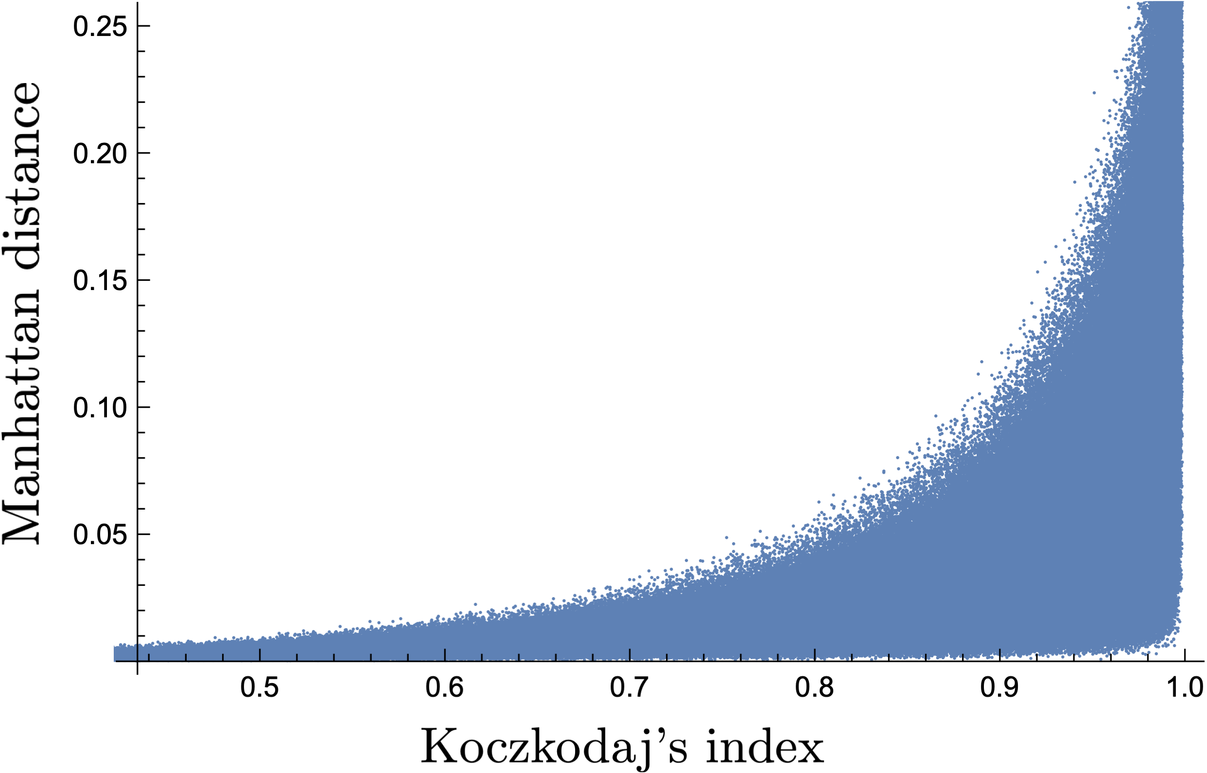
(a)

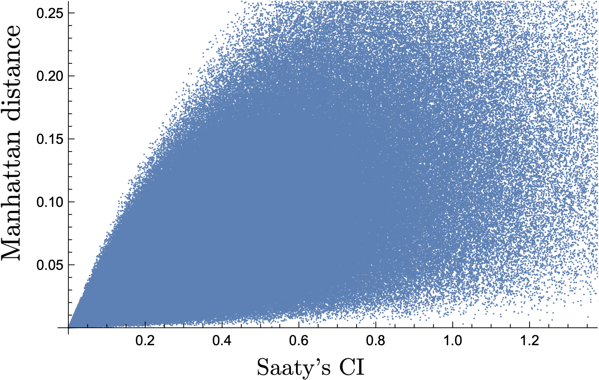
(b)

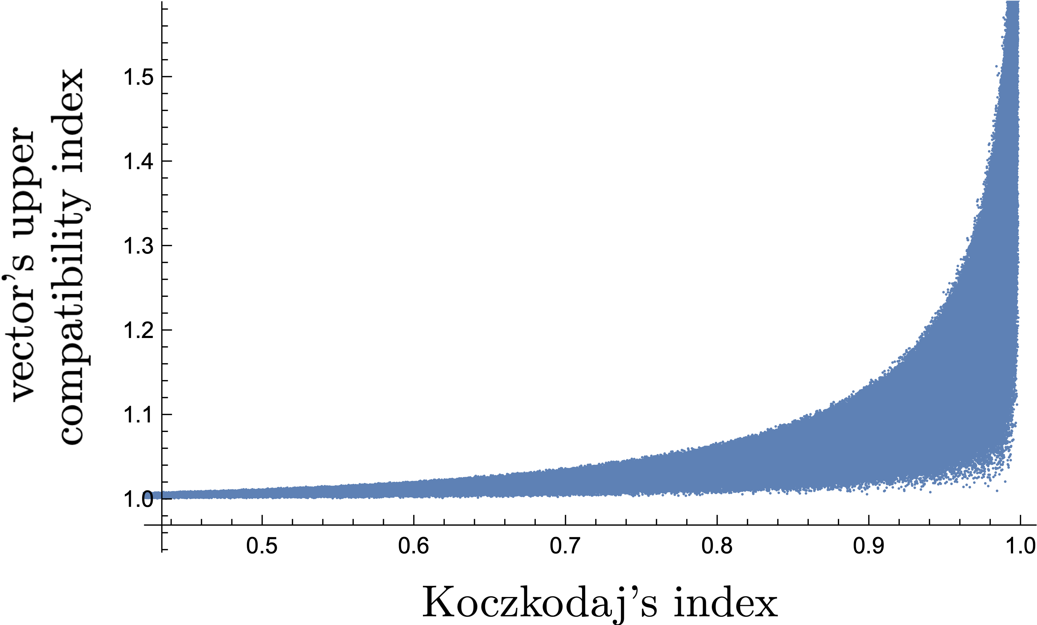
(c)

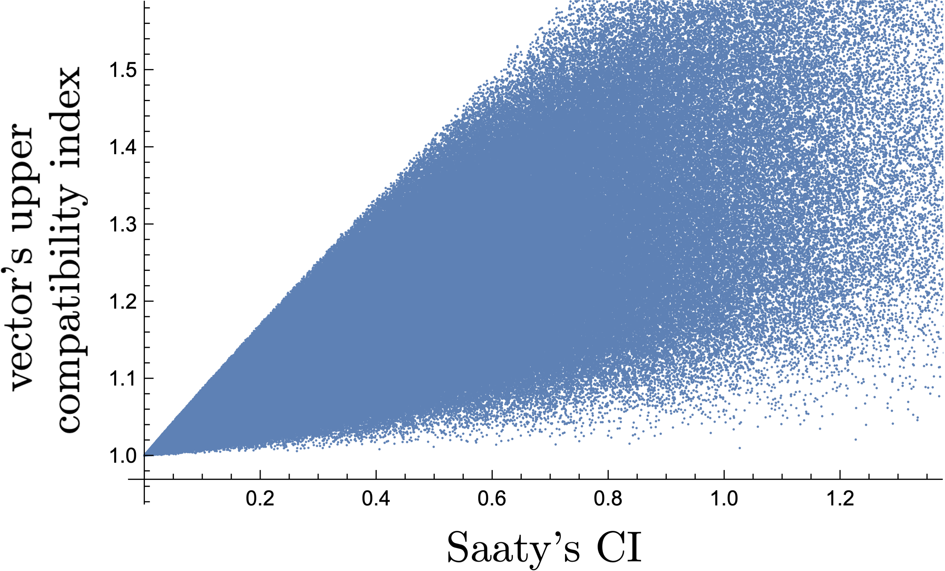
(d)

Figure 1: Manhattan distance and the vector’s upper compatibility index between the EVM and GMM ranking vectors obtained from the same PC matrix with a given inconsistency level.

The existence of these limitations is in line with the theoretical results shown above. An attentive reader will also notice that the theoretical maximum limitations resulting from Theorems 17, 18 and 19 are significantly stronger than the experimental results would suggest. This may mean that there are better estimates of the distance between the two ranking vectors representing the two most popular ranking algorithms for AHP. Trying to find them will pose a further challenge for researchers.

5 Summary

In the presented work, we returned to the matter of comparing the two main priority deriving methods in AHP. We proved the formal relationship of the distance between the ranking vectors calculated using the EVM and GMM methods with inconsistency.

In the presented assertions (Theorems 17, 18 and 19, Corollaries 20 and 21), to determine the inconsistency, we used Saaty’s and Koczkodaj’s indices, while the difference between the vectors was determined using Manhattan distance, Tchebyshev distance and compatibility indices (14). In order to compare the compatibility of two vectors, we adapted the concept of the matrix compatibility (Def. 10) and defined four new compatibility indices. Theorem 17 shows the relationship between the newly defined indices.

It is worth emphasizing that the perspective adopted in this article is purely quantitative. We do not deal with the qualitative comparison of ranking vectors, i.e. we do not study the order of alternatives. Instead, the proportions between the priorities of the alternatives are important to us. This approach is justified when the ranking is of quantitative importance, i.e. when the prize does not go only to the winner, but is distributed proportionally to the priority value among the competition participants. In such a situation, for small values of inconsistency indices, the differences between the EVM and GMM approaches are also small. Hence, from the perspective of a participant in the quantitative ranking, in a situation of low inconsistency, the choice of the priority deriving method is not so important. However, with higher values of inconsistency, it starts to matter. This result highlights once again how important it is to keep the inconsistency low.

Literature

References

- Barzilai [1997] J. Barzilai. Deriving weights from pairwise comparison matrices. The Journal of the Operational Research Society, 48(12):1226–1232, December 1997.
- Bozóki and Fülöp [2017] S. Bozóki and J. Fülöp. Efficient weight vectors from pairwise comparison matrices. European Journal of Operational Research, pages 419–427, September 2017.
- Brunelli [2018] M. Brunelli. A survey of inconsistency indices for pairwise comparisons. International Journal of General Systems, 47(8):751–771, September 2018.
- Brunelli [2019] M. Brunelli. A study on the anonymity of pairwise comparisons in group decision making. European Journal of Operational Research, 279(2):502–510, December 2019.
- Choo and Wedley [2004] E. U. Choo and W. C. Wedley. A common framework for deriving preference values from pairwise comparison matrices. Computers and Operations Research, 31(6):893 – 908, 2004. ISSN 0305-0548. doi: 10.1016/S0305-0548(03)00042-X. URL http://www.sciencedirect.com/science/article/pii/S030505480300042X.
- Colomer [2011] J. M. Colomer. Ramon Llull: from ‘Ars electionis’ to social choice theory. Social Choice and Welfare, 40(2):317–328, October 2011.
- Condorcet [1785] M. Condorcet. Essay on the Application of Analysis to the Probability of Majority Decisions. Paris: Imprimerie Royale, 1785.
- Crawford [1987] G. B. Crawford. The geometric mean procedure for estimating the scale of a judgement matrix. Mathematical Modelling, 9(3–5):327 – 334, 1987. ISSN 0270-0255. doi: http://dx.doi.org/10.1016/0270-0255(87)90489-1. URL http://www.sciencedirect.com/science/article/pii/0270025587904891.
- Crawford and Williams [1985] R. Crawford and C. Williams. A note on the analysis of subjective judgement matrices. Journal of Mathematical Psychology, 29:387 – 405, 1985.
- David [1969] H. A. David. The method of paired comparisons. A Charles Griffin Book, 1969.
- Fechner [1860] G. T. Fechner. Elemente der Psychophysik. Breitkopf und Härtel, Leipzig, 1860. URL https://archive.org/details/elementederpsych001fech.
- Gacula Jr. and Singh [1984] M. C. Gacula Jr. and J. Singh. Statistical Methods in Food and Consumer Research. Academic Press, December 1984.
- Gantmaher [2000] F. R. Gantmaher. The theory of matrices. American Mathematical Society, 2000.
- Golany and Kress [1993] B. Golany and M. Kress. A multicriteria evaluation of methods for obtaining weights from ratio-scale matrices. European Journal of Operational Research, 69(2):210–220, 1993.
- Harker [1987] P. T. Harker. Incomplete pairwise comparisons in the analytic hierarchy process. Mathematical Modelling, 9(11):837–848, 1987.
- Hefnawy and Mohammed [2014] E. A. Hefnawy and A. S. Mohammed. Review of different methods for deriving weights in The Analytic Hierarchy Process. International Journal of Analytic Hierarchy Process, 6(1):92 – 123, 2014.
- Herman and Koczkodaj [1996] M. W. Herman and W. W. Koczkodaj. A monte carlo study of pairwise comparison. Inf. Process. Lett., 57(1):25–29, January 1996. ISSN 0020-0190. doi: 10.1016/0020-0190(95)00185-9. URL http://dx.doi.org/10.1016/0020-0190(95)00185-9.
- Jablonsky [2015] J. Jablonsky. Analysis of selected prioritization methods in the analytic hierarchy process. Journal of Physics: Conference Series, 622(1):1–7, 2015.
- Kakiashvili et al. [2017] T. Kakiashvili, W. W. Koczkodaj, and J. P. Magnot. Approximate reasoning by pairwise comparisons. Physics of Life Reviews, 21:37–39, July 2017.
- Kendall [1938] M. G. Kendall. A new measure of rank correlation. Biometrika, 30(1/2):81, 1938.
- Koczkodaj [1993] W. W. Koczkodaj. A new definition of consistency of pairwise comparisons. Math. Comput. Model., 18(7):79–84, October 1993. ISSN 0895-7177. doi: 10.1016/0895-7177(93)90059-8. URL http://dx.doi.org/10.1016/0895-7177(93)90059-8.
- Kułakowski [2015] K. Kułakowski. On the properties of the priority deriving procedure in the pairwise comparisons method. Fundamenta Informaticae, 139(4):403 – 419, July 2015. doi: 10.3233/FI-2015-1240.
- Kułakowski and Kedzior [2016] K. Kułakowski and A. Kedzior. Some Remarks on the Mean-Based Prioritization Methods in AHP. In Ngoc-Thanh Nguyen, Lazaros Iliadis, Yannis Manolopoulos, and Bogdan Trawiński, editors, Lecture Notes In Computer Science, Computational Collective Intelligence: 8th International Conference, ICCCI 2016, Halkidiki, Greece, September 28-30, 2016. Proceedings, Part I, pages 434–443. Springer International Publishing, 2016. ISBN 978-3-319-45243-2. doi: 10.1007/978-3-319-45243-2-40. URL http://dx.doi.org/10.1007/978-3-319-45243-2-40.
- Kułakowski and Talaga [2020] K. Kułakowski and D. Talaga. Inconsistency indices for incomplete pairwise comparisons matrices. International Journal of General Systems, 49(2):174–200, 2020. doi: 10.1080/03081079.2020.1713116. URL https://doi.org/10.1080/03081079.2020.1713116.
- Kułakowski et al. [2019a] K. Kułakowski, J. Mazurek, J. Ramík, and M. Soltys. When is the condition of order preservation met? European Journal of Operational Research, 277(1):248–254, August 2019a.
- Kułakowski et al. [2019b] K. Kułakowski, J. Szybowski, and A. Prusak. Towards quantification of incompleteness in the pairwise comparisons methods. International Journal of Approximate Reasoning, 115:221–234, October 2019b.
- Mazurek and Ramík [2019] J. Mazurek and J. Ramík. Some new properties of inconsistent pairwise comparisons matrices. International Journal of Approximate Reasoning, 113:119–132, October 2019.
- Peterson and Brown [1998] G. L. Peterson and T. C. Brown. Economic valuation by the method of paired comparison, with emphasis on evaluation of the transitivity axiom. Land Economics, pages 240–261, 1998.
- Pinkerton and McAleer [1976] S. S. Pinkerton and C. A. McAleer. Influence of client diagnosis–cancer–on counselor decisions. Journal of Counceling Psychology, 23(6):575–578, 1976.
- Price [2017] L. R. Price. Psychometric Methods Theory into Practice. The Guilford Press, January 2017.
- Saari and Merlin [1996] D. G. Saari and V. R. Merlin. The Copeland method. Economic Theory, 8(1):51–76, February 1996.
- Saaty [1977] T. L. Saaty. A scaling method for priorities in hierarchical structures. Journal of Mathematical Psychology, 15(3):234 – 281, 1977. ISSN 0022-2496. doi: 10.1016/0022-2496(77)90033-5.
- Saaty [1980] T. L. Saaty. The analytic hierarchy process: planning, priority setting, resource allocation. McGrawHill International Book Co., New York; London, 1980. ISBN 0070543712 9780070543713.
- Saaty [2008] T. L. Saaty. Relative Measurement and Its Generalization in Decision Making. Why Pairwise Comparisons are Central in Mathematics for the Measurement of Intangible Factors. The Analytic Hierarchy/Network Process. Estadística e Investigación Operativa / Statistics and Operations Research (RACSAM), 102:251–318, November 2008.
- Suzumura et al. [2010] K. Suzumura, K. J. Arrow, and A. K. Sen. Handbook of Social Choice & Welfare. Elsevier Science Inc., 2010.
- Thurstone [1927] L. L. Thurstone. The Method of Paired Comparisons for Social Values. Journal of Abnormal and Social Psychology, pages 384–400, 1927.
- Thurstone [1994] L. L. Thurstone. A law of comparative judgment, reprint of an original work published in 1927. Psychological Review, 101:266–270, 1994.