22institutetext: Martinos Center for Biomedical Imaging, Harvard Medical School
Predictive Modeling of Anatomy
with Genetic and Clinical Data
Abstract
We present a semi-parametric generative model for predicting anatomy of a patient in subsequent scans following a single baseline image. Such predictive modeling promises to facilitate novel analyses in both voxel-level studies and longitudinal biomarker evaluation. We capture anatomical change through a combination of population-wide regression and a non-parametric model of the subject’s health based on individual genetic and clinical indicators. In contrast to classical correlation and longitudinal analysis, we focus on predicting new observations from a single subject observation. We demonstrate prediction of follow-up anatomical scans in the ADNI cohort, and illustrate a novel analysis approach that compares a patient’s scans to the predicted subject-specific healthy anatomical trajectory. The code is available at https://github.com/adalca/voxelorb.
Keywords:
neuroimaging, anatomical prediction, synthesis, simulation, genetics, generative model1 Introduction
We present a method for predicting anatomy based on external information, including genetic and clinical indicators. Specifically, given only a single baseline scan of a new subject in a longitudinal study, our model predicts anatomical changes and generates a subsequent image by leveraging subject-specific genetic and clinical information. Such voxel-wise prediction opens up several new areas of analysis, enabling novel investigations both at the voxel level and at the level of derivative biomarker measures. For example, voxel level differences between the true progression of a patient with dementia and their predicted healthy anatomy highlight spatial patterns of disease. We validate our method by comparing measurements of volumes of anatomical structures based on predicted images to those extracted from the acquired scans.
Our model describes the change from a single (or baseline) medical scan in terms of population trends and subject-specific external information. We model how anatomical appearance changes with age on average in a population, as well as deviations from the population average using a person’s health profile. We characterize such profiles non-parametrically based on the genotype, clinical information, and the baseline image. Subject-specific change is constructed from the similarity of health profiles in the cohort, using a Gaussian process parametrized by a population health covariance. Given the predicted change, we synthesize new images through an appearance model.
Statistical population analysis is one of the central topics in medical image computing. The classical correlation-based analysis has yielded important characterization of relationships within imaging data and with independent clinical variables [3, 13, 15, 17]. Regression models of object appearance have been previously used for atlas construction and population analysis [3, 17]. These methods characterize population trends with respect to external variables, such as age or gender, and construct clinically relevant population averages.
Longitudinal analyses also characterize subject-specific temporal effects, usually in terms of changes in the biomarkers of interest. Longitudinal cohorts and studies promise to provide crucial insights into aging and disease [13, 15]. Mixed effects models have been shown to improve estimation of subject-specific longitudinal trends by using inter-population similarity [4, 18]. While these approaches offer a powerful basis for analysis of biomarkers or images in a population, they require multiple observations for any subject, and do not aim to provide subject-specific predictions given a single observation. The parameters of the models are examined for potential scientific insight, but they are not tested for predictive power.
Recently, several papers have proposed prediction of medical images or specific anatomical structures by extrapolating at least two time points (e.g. a baseline and a follow-up image) to simulate a later follow-up measurement [2, 6]. These models, however, necessitate observations of at least two time points to make predictions which are difficult to acquire for every new patient. They are therefore not applicable to most patients, not applicable during a first visit, and are sensitive to noise in these few measurements. Recent methods have also used stratified population average deformations to make follow-up predictions from a baseline image [14]. While classified by population subgroups, these predictions are not adapted to a particular subject’s health or environment.
In contrast, we define the problem of population analysis as predicting anatomical changes for individual subjects. Our generative model incorporates a population trend and uses subject-specific genetic and clinical information, along with the baseline image, to generate subsequent anatomical images. This prediction-oriented approach provides avenues for novel analysis, as illustrated by our experimental results.
2 Prediction Model
Given a dataset of patients with longitudinal data, and a single baseline image for a new patient, we predict follow-up anatomical states for the patient. We model anatomy as a phenotype that captures the underlying structure of interest. For example, can be a low-dimensional descriptor of the anatomy at each voxel. We assume we only have a measurement of our phenotype at baseline for a new subject. Our goal is to predict the phenotype at a later time . We let be the subject age at time , and define and . We model the change in phenotype using linear regression:
| (1) |
where is the subject-specific regression coefficient, and noise is sampled from zero-mean Gaussian distribution with variance .
2.1 Subject-Specific Longitudinal Change
To model subject-specific effects, we define , where is a global regression coefficient shared by the entire population, and captures a deviation from this coefficient based on the subject’s genetic variants , clinical information , and baseline image features .
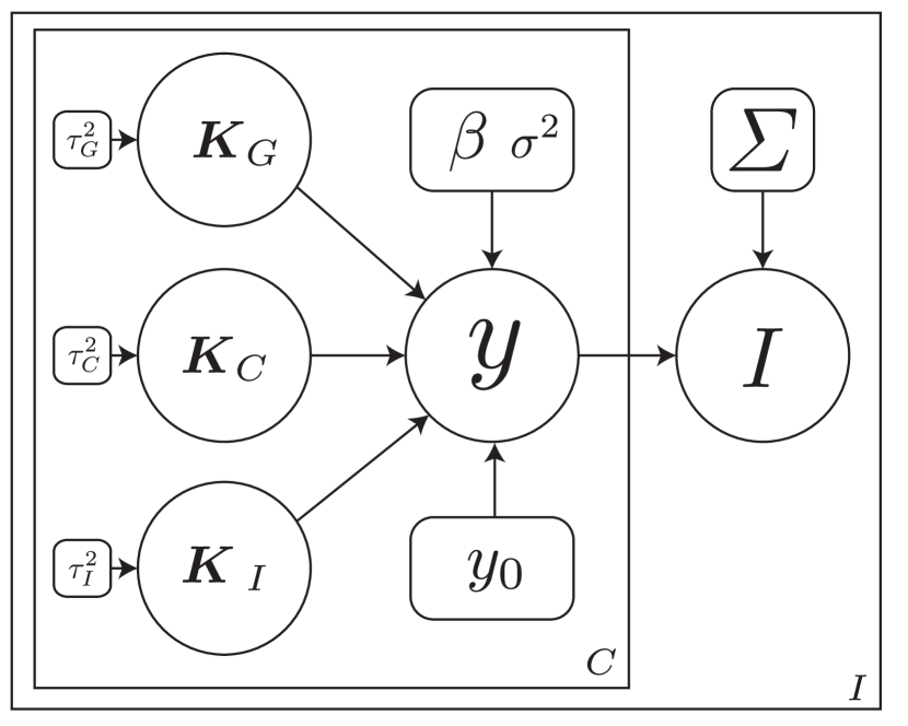
We assume that patients’ genetic variants and clinical indicators affect their anatomical appearance, and that subjects with similar health profiles exhibit similar patterns of anatomical change. We let , , be functions that capture genetic, clinical and imaging effects on the regression coefficients:
| (2) |
Combining with (1), we arrive at the full model
| (3) |
which captures the population trend , as well as the subject-specific deviations . Together with a description of an image from phenotype in the next section, equations (3) and (5) define a generative probabilistic interpretation of our model, which we show graphically in Figure 1.
For a longitudinal cohort of subjects, we group all observations for subject to form . We then form the global vector . We similarly form vectors , , , , , , and , to build the full regression model:
| (4) |
where is the Hadamard, or element-wise product. This formulation is mathematically equivalent to a General Linear Model (GLM) [11] in terms of the health profile predictors .
We employ Gaussian process priors to model the health functions:
| (5) |
where covariance kernel function captures the similarity between subjects and using feature vectors and for . We discuss the particular form of used in the experiments later in the paper.
2.2 Learning
The Bayesian formulation in (4) and (5) can be interpreted as a linear mixed effects model (LMM) [12] or a least squares kernel machine (LSKM) regression model [7, 10]. We use the LMM interpretation to learn the parameters of our model, and the LSKM interpretation to perform final phenotype predictions.
Specifically, we treat as the coefficient vector of fixed effects and , and as independent random effects. We seek the maximum likelihood estimates of parameters and by adapting standard procedures for LMMs [7, 10]. As standard LMM solutions become computationally expensive for thousands of observations, we take advantage of the fact that while the entire genetic and the image phenotype data is large, the use of kernels on baseline data reduces the model size substantially. We obtain intuitive iterative updates that project the residuals at each step onto the expected rate of change in likelihood, and update using the best linear unbiased predictor.
2.3 Prediction
Under the LSKM interpretation, the terms are estimated by minimizing a penalized squared-error loss function, which leads to the following solution [7, 9, 10, 19]:
| (6) |
for some vector . Combining with the definitions of the LMM, we estimate coefficients vectors and from a linear system of equations that involves our estimates of and . We can then re-write (4) as
| (7) |
and predict a phenotype at time for a new subject :
| (8) |
3 Model Instantiation for Anatomical Predictions
The full model (3) can be used with many reasonable phenotype definitions. Here, we describe the phenotype model we use for anatomical predictions and specify the similarity kernels of the health profile.
3.1 Anatomical Phenotype
We define a voxel-wise phenotype that enables us to predict entire anatomical images. Let be the set of all spatial locations (voxels) in an image, and be the acquired baseline image. We similarly define , to be the population atlas template. We assume each image is generated through a deformation field parametrized by the corresponding displacements from the common atlas to the subject-specific coordinate frame [17], such that We further define a follow-up image as a deformation from the baseline image , which can be composed to yield an overall deformation from the atlas to the follow-up scan via :
| (9) |
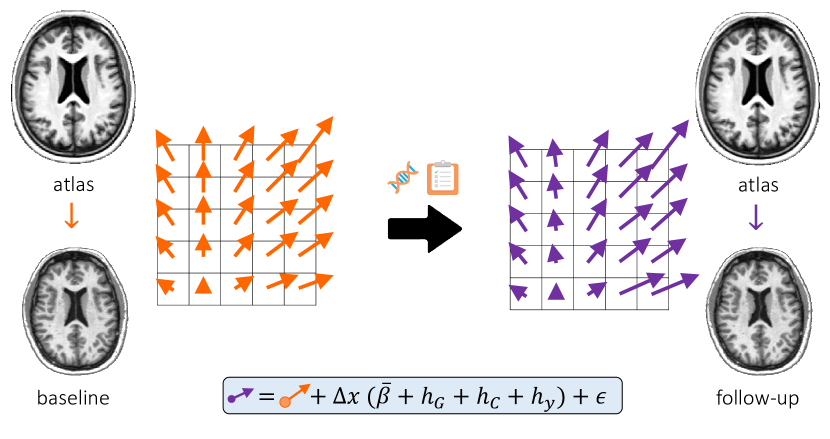
Using displacements as the phenotype of interest in (1) captures the necessary information for predicting new images, but leads to very high dimensional descriptors. To regularize the transformation and to improve efficiency, we define a low-dimensional embedding of . Specifically, we assume that the atlas provides a parcellation of the space into L anatomical labels . We build a low-dimensional embedding of the transformation vectors within each label using PCA. We define the relevant phenotypes as the coefficients associated with the first principal components of the model that capture 95% of the variance in each label, for .
We predict the phenotypes using (8). To construct a follow-up image given phenotype , we first form a deformation field by reconstruction from the estimated phenotype , and use assuming an invertible transformation. Using the baseline image, we predict a subsequent image via . Note that we do not directly model changes in image intensity. While population models necessitate capturing such changes, we predict changes from a baseline image. We also assume that affine transformations are not part of the deformations of interest, and thus all images are affinely registered to the atlas.
3.2 Health Similarities
To fully define the health similarity term , we need to specify the forms of the kernel functions , , and .
For genetic data, we employ the identical by state (IBS) kernel often used in genetic analysis [16]. Given a vector of genetic variants of length , each genetic locus is encoded as , and
| (10) |
To capture similarity of clinical indicators , we form the kernel function
| (11) |
where diagonal weight matrix captures the effect size of each clinical indicator on the phenotype, and is the variance of the clinical factors.
We define the image feature vectors as the set of all PCA coefficients defined above for the baseline image. We define the image kernel matrix as
| (12) |
where is the variance of the image features.
We emphasize that other data sources can easily be incorporated in the model by simply adding appropriate kernels for that data.
4 Experiments


We illustrate our approach by predicting image-based phenotypes based on genetic, clinical and imaging data in the ADNI longitudinal study [8] that includes two to ten follow-up scans acquired years after the baseline scan. We use affine registration to align all subjects to a template constructed from randomly chosen subjects, and compute non-linear registration warps for each image using ANTs [1]. We utilize a list of genetic loci associated with Alzheimer’s disease (AD) as the genetic vector , and the standard clinical factors including age, gender, marital status, education, disease diagnostic, and cognitive tests, as the clinical indicator vector . We learn the model parameters from 341 randomly chosen subjects and predict follow-up volumes on a separate set of 100 subjects. To evaluate the advantages of the proposed predictive model, we compare its performance to a population-wide linear regression model that ignores the subject-specific health profiles (i.e., ).
4.1 Volumetric Predictions
In the first simplified experiment, we define phenotype to be a vector of several scalar volume measurements obtained using FreeSurfer [5]. In addition to the population-wide linear regression model, we include a simple approach of using the baseline volume measurements as a predictor of the phenotype trajectory, effectively assuming no volume change with time. Since in many subjects, the volume differences are small, all three methods perform comparably when evaluated on the whole test set. To evaluate the differences between the methods, we focus on the subset of subjects with substantial volume changes, reported in Fig. 3. Our method consistently achieves smaller relative errors than the two baseline approaches.
4.2 Anatomical Prediction
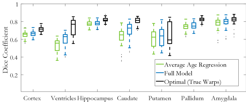
We also evaluate the model for full anatomical scan prediction. An example prediction is shown in Fig. 4. To quantify prediction accuracy, we propagate segmentation labels of relevant anatomical structures from the baseline scan to the predicted scan using the predicted warps. We compare the predicted segmentation label maps with the actual segmentations of the follow-up scans. The warps computed based on the actual follow-up scans through the atlas provide an indication of the best accuracy the predictive model could achieve when using warps to represent images. Similar to the volumetric predictions, the full model offers modest improvements when evaluated on the entire test set, and substantial improvements in segmentation accuracy when evaluated in the subjects who exhibit large volume changes between the baseline scan and the follow-up scan, as reported in Fig. 5 and exemplified in Fig. 6. In both experiments, all components and contributed significantly to the improved predictions.

Our experimental results suggest that the anatomical model depends on registration accuracy. In particular, we observe that directly registering the follow-up scan to the baseline scan leads to better alignment of segmentation labels than when transferring the labels through a composition of the transformations from the scans to the atlas space. This suggests that a different choice of appearance model may improve prediction accuracy, a promising direction for future work.
4.3 Example Application
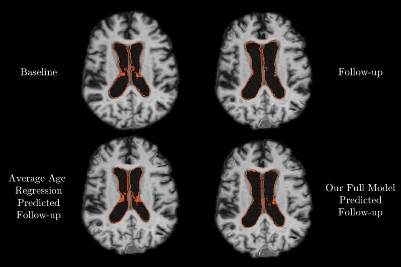
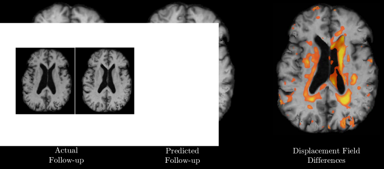
To demonstrate the potential of the anatomical prediction, we predict the follow-up scan of a patient diagnosed with dementia as if the patient were healthy. Specifically, we train our model using healthy subjects, and predict follow-up scans for AD patients. In Fig. 7 we illustrate an example result, comparing the areas of brain anatomy that differ from the observed follow-up in the predicted healthy brain of this AD patient. Our prediction indicates that ventricle expansion would be different if this patient had a healthy trajectory.
5 Conclusions
We present a model to predict the anatomy in patient follow-up images given just a baseline image using population trends and subject-specific genetic and clinical information. We validate our prediction method on scalar volumes and anatomical images, and show that it can be used as a powerful tool to illustrate how a subject-specific brain might differ if it were healthy. Through this and other new applications, our prediction method presents a novel opportunity for the study of disease and anatomical development.
Acknowledgements. We acknowledge the following funding sources: NIH NIBIB 1K25EB013649-01, BrightFocus AHAF-A2012333, NIH NIBIB NAC P41EB015902, NIH DA022759, and Wistron Corporation.
References
- [1] Avants, B., Tustison, N., Song, G., Cook, P., Klein, A., Gee, J.: A reproducible evaluation of ants similarity metric performance in brain image registration. Neuroimage 54(3), 2033–2044 (2011)
- [2] Blanc, R., Seiler, C., Székely, G., Nolte, L.P., Reyes, M.: Statistical model based shape prediction from a combination of direct observations and various surrogates: application to orthopaedic research. Med Image Anal 16(6), 1156–1166 (2012)
- [3] Davis, B.C., Fletcher, P.T., Bullitt, E., Joshi, S.: Population shape regression from random design data. Int J Comp. Vis. 90(2), 255–266 (2010)
- [4] Durrleman, S., Pennec, X., Trouvé, A., Braga, J., Gerig, G., Ayache, N.: Toward a comprehensive framework for the spatiotemporal statistical analysis of longitudinal shape data. International journal of computer vision 103(1), 22–59 (2013)
- [5] Fischl, B.: Freesurfer. Neuroimage 62(2), 774–781 (2012)
- [6] Fleishman, G.M., Gutman, B.A., Fletcher, P.T., Thompson, P.M.: Simultaneous longitudinal registration with group-wise similarity prior. Information Processing in Medical Imaging LNCS 9123, 746–757 (2015)
- [7] Ge, T., Nichols, T.E., Ghosh, D., Mormino, E.C., Smoller, J.W., Sabuncu, M.R., et al.: A kernel machine method for detecting effects of interaction between multidimensional variable sets: An imaging genetics application. NeuroImage (2015)
- [8] Jack, C.R., Bernstein, M.A., Fox, N.C., Thompson, P., Alexander, G., Harvey, D., Borowski, B., Britson, P.J., L Whitwell, J., Ward, C., et al.: The alzheimer’s disease neuroimaging initiative (adni): Mri methods. Journal of Magnetic Resonance Imaging 27(4), 685–691 (2008)
- [9] Kimeldorf, G., Wahba, G.: Some results on tchebycheffian spline functions. Journal of mathematical analysis and applications 33(1), 82–95 (1971)
- [10] Liu, D., Lin, X., Ghosh, D.: Semiparametric regression of multidimensional genetic pathway data: Least-squares kernel machines and linear mixed models. Biometrics 63(4), 1079–1088 (2007)
- [11] McCullagh, P.: Generalized linear models. European Journal of Operational Research 16(3), 285–292 (1984)
- [12] McCulloch, C.E., Neuhaus, J.M.: Generalized linear mixed models. Wiley Online Library (2001)
- [13] Misra, C., Fan, Y., Davatzikos, C.: Baseline and longitudinal patterns of brain atrophy in mci patients, and their use in prediction of short-term conversion to ad: results from adni. Neuroimage 44(4), 1415–1422 (2009)
- [14] Modat, M., Simpson, I.J., Cardoso, M.J., Cash, D.M., Toussaint, N., Fox, N.C., Ourselin, S.: Simulating neurodegeneration through longitudinal population analysis of structural and diffusion weighted mri data. MICCAI: International Conference on Medical Image Computing and Computer-Assisted Intervention LNCS 8675, 57–64 (2014)
- [15] Pfefferbaum, A., Rohlfing, T., Rosenbloom, M.J., Chu, W., Colrain, I.M., Sullivan, E.V.: Variation in longitudinal trajectories of regional brain volumes of healthy men and women (ages 10 to 85years) measured with atlas-based parcellation of mri. Neuroimage 65, 176–193 (2013)
- [16] Queller, D.C., Goodnight, K.F.: Estimating relatedness using genetic markers. Evolution pp. 258–275 (1989)
- [17] Rohlfing, T., Sullivan, E.V., Pfefferbaum, A.: Regression models of atlas appearance. In: Prince, J.L., Pham, D.L., Myers, K.J. (eds.) Info. Proc. Med. Img. pp. 151–162. Springer (2009)
- [18] Sadeghi, N., Prastawa, M., Fletcher, P.T., Vachet, C., Wang, B., et al.: Multivariate modeling of longitudinal mri in early brain development with confidence measures. In: 2013 IEEE Inter. Symp. Biomed Imag. pp. 1400–1403. IEEE (2013)
- [19] Wahba, G.: Spline models for observational data, vol. 59. Siam (1990)