Compensated Convex Based Transforms
for Image Processing and Shape Interrogation

Abstract

This paper reviews some recent applications of the theory of the compensated convex transforms or of the proximity hull as developed by the authors to image processing and shape interrogation with special attention given to the Hausdorff stability and multiscale properties. The paper contains also numerical experiments that demonstrate the performance of our methods compared to the state-of-art ones.

Keywords:Compensated convex transform, Moreau envelope, Proximity hull, Mathematical morpohlogy, Hausdorff-Lipschitz continuity, Image processing, Shape interrogation, Scattered data

2000 Mathematics Subjects Classification number: 90C25, 90C26, 49J52, 52A41, 65K10, 62H35, 14J17, 58K25, 53-XX, 65D17, 53A05, 26B25, 52B55, 65D18

Email: aorlando@herrera.unt.edu.ar, e.c.m.crooks@swansea.ac.uk, kewei.zhang@nottingham.ac.uk

1 Introduction

The compensated convex transforms were introduced in [116, 117] for the purpose of tight approximation of functions defined in $\mathbb{R}^{n}$ and their definitions were originally motivated by the translation method [76, 50, 54, 105] in the study of the quasiconvex envelope in the vectorial calculus of variations (see [45, 115] and references therein) and in the variational approach of material microstructure [19, 20, 21]. Thanks to their smoothness and tight approximation property, these transforms provide geometric convexity-based techniques for general functions that yield novel methods for identifying singularities in functions [122, 123, 118, 120] and new tools for function and image interpolation and approximation [119, 121]. In this paper we present some of the applications that have been tackled by this theory up to date. These range from the detection of features in images or data [122, 123, 120], to multi-scale medial-axis extraction [118], to surface reconstruction from level sets, to approximation of scattered data and noise removal from images, to image inpainting [119, 121].

Suppose $f:\mathbb{R}^{n}\to\mathbb{R}$ satisfies the following growth condition

$$f(x)\geq-A_{1}|x|^{2}-A_{2}\quad\text{ for any }x\in\mathbb{R}^{n}\,,$$ (1.1)

for some constants $A_{1},\,A_{2}\geq 0$, then the quadratic lower compensated convex transform (lower transform for short) for a given $\lambda>A_{1}$ is defined in [116] by

$$C^{l}_{\lambda}(f)(x)=\operatorname{\mathsf{co}}\left[\lambda|\cdot|^{2}+f\right](x)-\lambda|x|^{2}\qquad x\in\mathbb{R}^{n},$$ (1.2)

where $|x|$ is the Euclidean norm of $x\in\mathbb{R}^{n}$ and $\operatorname{\mathsf{co}}[g]$ the convex envelope [58, 88] of a function $g:\mathbb{R}^{n}\to\mathbb{R}$ bounded below. Similarly, given $f:\mathbb{R}^{n}\to\mathbb{R}$ satisfying the growth condition

$$f(x)\leq A_{1}|x|^{2}+A_{2}\quad\text{ for any }x\in\mathbb{R}^{n}\,,$$ (1.3)

for some constants $A_{1},\,A_{2}\geq 0$, the quadratic upper compensated convex transform (upper transform for short) for a given $\lambda>A_{1}$ is defined [116] by

$$\begin{split}C^{u}_{\lambda}(f)(x)&=-C^{l}_{\lambda}(-f)(x)\\[6.45831pt] &=\lambda|x|^{2}-\operatorname{\mathsf{co}}\left[\lambda|\cdot|^{2}-f\right](x)\qquad x\in\mathbb{R}^{n}\,.\end{split}$$ (1.4)

It is not difficult to verify that if $f$ meets both (1.1) and (1.3), for instance if $f$ is bounded, there holds

$$C^{l}_{\lambda}(f)(x)\leq f(x)\leq C^{u}_{\lambda}(f)(x)\quad x\in\mathbb{R}^{n}\,,$$

thus, the lower and upper compensated convex transforms are $\lambda$-parametrised families of transforms that approximate $f$ from below and above respectively. Furthermore, they have smoothing effects and are tight approximations of $f$ in the sense that if $f$ is $C^{1,1}$ in a neighbourhood of $x_{0}$, there is a finite $\Lambda>0$, such that $f(x_{0})=C^{l}_{\lambda}(f)(x_{0})$ (respectively, $f(x_{0})=C^{u}_{\lambda}(f)(x_{0})$ whenever $\lambda\geq\Lambda$. This approximation property, which we refer to as tight approximation, is pivotal in the developments of the theory, because it allows the transforms to be used for detecting singularities of functions by exploiting the fact that it is only when a point $x$ is close to a singularity point of $f$ we might find that the values of $C^{l}_{\lambda}(f)(x)$ and $C^{u}_{\lambda}(f)(x)$ might be different from that of $f(x)$ [122]. Figure 1 visualizes the smoothing and tight approximation of the mixed transform $C^{u}_{\lambda}(C^{l}_{\lambda}(f))$ of the squared distance function $f$ to a four-point set. Given the type of singularity of $f$, we apply the lower transform to $f$ which smooth the ‘concave’–like singularity followed by the upper transform that smoothes the ‘convex’–like singularity of $C^{l}_{\lambda}(f)$ which are unalterated with respect to the original function $f$. This can be appreciated by the graph of the pointwise error $e(x)=|f(x)-C_{\lambda}^{u}(C_{\lambda}^{l}(f))(x)|$ for $x\in\Omega$ which is zero everywhere but in a neighborhood of the singularities of $f$.

$\begin{array}[]{ccc}\includegraphics[width=112.67548pt]{Dist4pntGraphCntr.png}&\includegraphics[width=112.67548pt]{Dist4pntGraphLmbd5GraphUpLwTrCnt.png}&\includegraphics[width=112.67548pt]{Dist4pntGraphLmbd5GraphErr.png}\\ (a)&(b)&(c)\end{array}$

Figure 1: Graph of $(a)$ a squared distance function $f$ to a four-point set, $(b)$ its mixed transform $C_{\lambda}^{u}(C_{\lambda}^{l}(f))$ and $(c)$ the pointwise error $e=|f-C_{\lambda}^{u}(C_{\lambda}^{l}(f))|$.

The transforms additionally satisfy the locality property that the values of $C^{l}_{\lambda}(f)$, $C^{u}_{\lambda}(f)$ at $x\in\mathbb{R}^{n}$ depend only on the values of $f$ in a neighbourhood of $x$, and are translation invariant in the sense that $C^{l}_{\lambda}(f)$, $C^{u}_{\lambda}(f)$ are unchanged if the ‘weight’ $|\cdot|^{2}$ in the formula (1.2) and (1.4) is replaced by $|\cdot-x_{0}|^{2}$ for any shift $x_{0}\in\mathbb{R}^{n}$. These last two properties make the explicit calculation of transforms tractable for specific prototype functions $f$, which facilitates the creation of dedicated extractors for a variety of different types of singularity using customised combinations of the transforms.

These new geometric approaches enjoy key advantages over previous image and data processing techniques [17, 37, 95, 110]. The curvature parameter $\lambda$ provides scales for features that allow users to select which size of feature they wish to detect, and the techniques are blind and global, in the sense that images/data are treated as a global object with no a priori knowledge required of, e.g., feature location. Figure 2 displays the $\lambda-$scale dependence in the case of the medial axis where $\lambda$ is associated with the scale of the different branches whereas Figure 3 shows the multiscale feature for given $\lambda$ associated with the height of the different branches of the multiscale medial axis map.

$\begin{array}[]{cc}\includegraphics[width=164.31752pt]{zhengkaiLmbd1Lev2_55e-06MatLabThin.png}&\includegraphics[width=164.31752pt]{zhengkaiLmbd8Lev2_55e-06MatLabThin.png}\\ (a)&(b)\end{array}$

Figure 2: Support of the multiscale medial axis map (suplevel set with level $t=10^{-8}\max_{x\in\mathbb{R}^{2}}\,{M_{\lambda}(\cdot;K)}$) with the ‘spurious’ branches generated by pixelation of the boundary for $(a)$ $\lambda=1$ and for $(b)$ $\lambda=8$.

$\begin{array}[]{cc}\includegraphics[width=164.31752pt]{zhengkaiLmbd1Lev0_255MatLabThin.png}&\includegraphics[width=164.31752pt]{zhengkaiLmbd1Lev5MatLabThin.png}\\ (a)&(b)\end{array}$

Figure 3: Selection of branches via the suplevel set of the multiscale medial axis map for $\lambda=1$ using different values of the threshold $t$, $(a)$ $t=10^{-3}\max_{x\in\mathbb{R}^{2}}\,{M_{\lambda}(\cdot;K)}$ and $(b)$ $t=2\cdot 10^{-2}\max_{x\in\mathbb{R}^{2}}\,{M_{\lambda}(\cdot;K)}$.

Many of the methods can also be shown to be stable under perturbation and different sampling techniques. Most significantly, Hausdorff stability results can be rigorously proved for many of the methods. For example, the Hausdorff-Lipschitz continuity estimate [122]

$$|C^{u}_{\lambda}(\chi_{E})(x)-C^{u}_{\lambda}(\chi_{F})(x)|\leq 2\sqrt{\lambda}\mathrm{dist}_{\mathcal{H}}(E,F),\;\;\;x\in\mathbb{R}^{n},$$

shows that the upper transform $C^{u}_{\lambda}$ is Hausdorff stable against sampling of geometric shapes defined by their characteristic functions. Such stability is particularly important for the extraction of information when ‘point clouds’ represent sampled domains. If a geometric shape is densely sampled, then from a human vision point of view, one can typically still identify geometric features of the sample and sketch its boundary. From the mathematical/computer science perspective, however, feature identification from sampled domains is challenging and usually methods are justified only by either ad hoc arguments or numerical experiments. Figure 4 displays an instance of this property where we show the edges of the continuous nonnegative function $f(x,y)=\mathrm{dist}^{2}((x,y),\,\partial\Omega)$, with $(x,y)\in\Omega=([-1.5,\,1.5]\times[-1.5,\,1.5])\setminus([-1.5,\,0.5]\times[-1.5,\,-0.5])$, and of its sparse sampling $f\cdot\chi_{A}$ where $A\subset\Omega$ is a sparse set (see Figure 4$(a)$, $(b)$ respectively). Due to the Hausdorff stability of the stable ridge transform, we are able to recover an approximation of the ridges from the sampled image (compare Figure 4$(c)$, $(d)$).

$\begin{array}[]{cccc}\includegraphics[width=112.67548pt]{LshapeDistTransf.png}&\includegraphics[width=112.67548pt]{LshapeDistTransfSamplingDNS0_3.png}&\includegraphics[width=112.67548pt]{LshapeDistTransfRidgeLmbd1.png}&\includegraphics[width=112.67548pt]{LshapeDistTransfSamplingDNS0_3StabRidgLmbd1.png}\\ (a)&(b)&(c)&(d)\end{array}$

Figure 4: $(a)$ Image of $f(x,y)$; $(b)$ Sampled image of $f(x,y)$ by random salt and pepper noise; $(c)$ Stable ridges of $f(x,y)$; $(d)$ Stable ridges from sampled image.

Via fast and robust numerical implementations of the transforms [124], this theory also gives rise to a highly-effective computational toolbox for applications. The efficiency of the numerical computations benefits greatly from the locality property, which holds despite the global nature of the convex envelope itself.

Before we describe the applications of this theory, we provide next alternative characterizations of the compensated convex transforms.

1.1 Related areas: Semiconvex envelope

Given the definitions (1.2) and (1.4), lower and upper compensated convex transforms can be considered as parameterized semiconvex and semiconcave envelopes, respectively, for a given function. The notions of semiconvex and semiconcave functions go back at least to Reshetnyak [87] and have since been studied by many authors in different contexts (see, for example, [5, 6, 31, 66, 89, 111]). Let $\Omega\subseteq\mathbb{R}^{n}$ be an open set, we recall that a function $f:\Omega\to\mathbb{R}\cup\{+\infty\}$ is semiconvex if there is a constant $C\geq 0$ such that $f(x)=g(x)-C|x|^{2}$ with $g$ a convex function. More general weight functions, such as $|x|\sigma(|x|)$, for example, are also used in the literature for defining more general semiconvex functions [5, 6, 18, 91, 92]. Since general DC-functions (difference of convex functions) [56] and semiconvex/semiconcave functions are locally Lipschitz functions in their essential domains ([31, Theorem 2.1.7]), Rademacher’s theorem implies that they are differentiable almost everywhere. Fine properties for the singular sets of convex/concave and semiconvex/semiconcave functions have been studied extensively [6, 3, 31] showing that the singular set of a semiconvex/semiconcave function is rectifiable. By applying results and tools of the theory of compensated convex transforms, it is possible therefore to study how such functions can be effectively approximated by smooth functions, whether all singular points are of the same type, that is, for semiconcave (semiconvex) functions, whether all singular points are geometric ‘ridge’ (‘valley’) points, how singular sets can be effectively extracted beyond the definition of differentiability and how the information concerning ‘strengths’ of different singular points can be effectively measured. These are all questions relevant to applications in image processing and computer-aided geometric design. An instance of this study, for example, has been carried out in [118, 120] to study the singular set of the Euclidean squared-distance function $\mathrm{dist}^{2}(\cdot,\Omega^{c})$ to the complement of a bounded open domain $\Omega\subset\mathbb{R}^{n}$ (called the medial axis [24] of the domain $\Omega$) and of the weighted squared distance function [79].

1.2 Related areas: Proximity hull

Another characterization of the compensated convex transforms is in terms of the critical mixed Moreau envelopes, given that

$$C^{l}_{\lambda}(f)(x)=M^{\lambda}(M_{\lambda}(f))(x)\,,\qquad C^{u}_{\lambda}(f)(x)=M_{\lambda}(M^{\lambda}(f))(x)\,,$$ (1.5)

where the Moreau lower and upper envelopes [77, 78] are defined, in our notation, respectively, by

$$\begin{array}[]{l}\displaystyle M_{\lambda}(f)(x)=\inf\{f(y)+\lambda|y-x|^{2},\;y\in\mathbb{R}^{n}\}\,,\\[6.45831pt] \displaystyle M^{\lambda}(f)(x)=\sup\{f(y)-\lambda|y-x|^{2},\;y\in\mathbb{R}^{n}\}\,,\end{array}$$ (1.6)

with $f$ satisfying the growth condition (1.1) and (1.3), respectively. Moreau envelopes play important roles in optimization, nonlinear analysis, optimal control and Hamilton-Jacobi equations, both theoretically and computationally [44, 31, 58, 90]. The mixed Moreau envelopes $M^{\tau}(M_{\lambda}(f))$ and $M_{\tau}(M^{\lambda}(f))$ coincide with the Lasry-Lions double envelopes $(f_{\lambda})^{\tau}$ and $(f^{\lambda})_{\tau}$ defined in [66] by (2.5) and (2.6), respectively, in the case of $\lambda=\tau$ and are also referred to in [104, 90] as proximal hull and upper proximal hull, respectively. They have been extensively studied and used as approximation and smoothing methods of not necessarily convex functions [16, 31, 82, 55]. In particular, in the partial differential equation literature, the focus of the study of the mixed Moreau envelopes $M^{\tau}(M_{\lambda}(f))$ and $M_{\tau}(M^{\lambda}(f))$ for the case $\tau>\lambda$ are known, under suitable growth conditions, as the Lasry-Lions regularizations of $f$ of parameter $\lambda$ and $\tau$. In this case, the mixed Moreau envelopes are both $C^{1,1}$ functions [16, 31, 66]. However, crucially they are not ‘tight approximations’ of $f$, in contrast with our lower and upper transforms $C^{l}_{\lambda}(f)(x)$ and $C^{u}_{\lambda}(f)(x)$ [116]. Generalised $\inf$ and $\sup$ convolutions have also been considered, for instance in [31, 90]. However, due to the way these regularization operators are defined, proof of mathematical and geometrical results to describe how such approximations work has usually been challenging, making their analysis and applications very difficult. As a result, the study of the proximal hull using the characterization in terms of the compensated convex transform would make them much more accesible and feasible for real world applications.

1.3 Related areas: Mathematical morphology

Moreau lower and upper envelopes have also been employed in mathematical morphology in the 1990’s [60, 108], to define greyscale erosion and dilation morphological operators, whereas the critical mixed Moreau envelopes $M^{\lambda}(M_{\lambda}(f))$ and $M_{\lambda}(M^{\lambda}(f))$ are greyscale opening and closing morphological operators [96, 102, 98]. In convex analysis, the infimal convolution of $f$ with $g$ is denoted as $f\Box g$ and is defined as [88, 23, 41, 90]

$$(f\Box g)(x)=\underset{y}{\inf}\,\{f(y)+g(x-y)\}\,.$$

This is closely related to the erosion of $f$ by $g$, given that

$$(f\Box g)(x)=f(x)\ominus(-g(-x))\,.$$

Thus if we denote by $b_{\lambda}(x)=-\lambda|x|^{2}$ the quadratic structuring function, introduced for the first time in [60, 107, 63, 61, 62], then with the notation of [96, 102, 98, 8], we have

$$\begin{array}[]{l}\displaystyle M_{\lambda}(f)(x)=\underset{y\in\mathbb{R}^{n}}{\inf}\{f(y)-b_{\lambda}(y-x)\}=:f\ominus b_{\lambda}\,,\\[6.45831pt] \displaystyle M^{\lambda}(f)(x)=\underset{y\in\mathbb{R}^{n}}{\sup}\{f(y)+b_{\lambda}(y-x)\}=:f\oplus b_{\lambda}\end{array}$$ (1.7)

so that (1.5) can be written alternatively as

$$C_{\lambda}^{l}(f)=(f\ominus b_{\lambda})\oplus b_{\lambda}\quad\text{and}\quad C_{\lambda}^{u}(f)=(f\oplus b_{\lambda})\ominus b_{\lambda}\,.$$ (1.8)

The application of $M^{\lambda}(M_{\lambda}(f))$ and $M_{\lambda}(M^{\lambda}(f))$ in mathematical morphology [96, 102, 98], however, has not met with corresponding success, nor have its properties been fully explored. This is in contrast with the rôle, recognized since its introduction, that is played by paraboloid structuring functions in defining morphological scale-spaces in image analysis [60, 107, 94, 68, 69, 74, 74, 113, 112]. For this and related topics concerning the morphological scale-space representation produced by quadratic structuring functions, we refer to the pionering works [60, 107]. Here, we would like only to observe that through identity (1.5), we have a direct characterization of the quadratic structuring based opening and closing morphological operators, either in terms of the convex envelope (see (1.2) and (1.4)) or in terms of envelope from below/above with parabolas (see (1.9) and (1.10)). Such characterizations will allow us to derive various new geometric and stability properties for the opening and closing morphological operators. Furthermore, when we apply compensated convex transforms to extract singularities from characteristic functions of compact geometric sets, our operations can be viewed as the application of morphological operations devised for ‘greyscale images’ to ‘binary images’. As a result, it might look not efficient to apply more involved operations for processing binary images, when in the current literature [96, 102, 98] there are ‘binary’ set theoretic morphological operations that have been specifically designed for the tasks under examination. Nevertheless, an advantage of adopting our approach is that the compensated convex transforms of characteristic functions are (Lipschitz) continuous, therefore applying a combination of transforms will produce a landscape of various levels (heights) that can be designed to highlight a specific type of singularity. We can then extract multiscale singularities by taking thresholds at different levels. In fact, the graphs of functions obtained by combinations of compensated convex transforms contain much more geometric information than binary operations that produce simply a yes or no answer. Also, for ‘thin’ geometric structures, such as curves and surfaces, it is difficult to design ‘binary’ morphological operations to be Hausdorff stable.

1.4 Related areas: Quadratic envelopes

From definition (1.2), it also follows that $C^{l}_{\lambda}(f)(x)$ is the envelope of all the quadratic functions with fixed quadratic term $\lambda|x|^{2}$ that are less than or equal to $f$, that is,

$$C^{l}_{\lambda}(f)(x)=\sup\left\{-\lambda|x|^{2}+\ell(x):\;-\lambda|y|^{2}+\ell(y)\leq f(y)\;\;\text{\rm for all }y\in\mathbb{R}^{n}\;\;\text{\rm and }\ell\;\;\text{\rm affine}\right\}\,,$$ (1.9)

whereas from (1.4) it follows that $C^{u}_{\lambda}(f)(x)$ is the envelope of all the quadratic functions with fixed quadratic term $\lambda|x|^{2}$ that are greater than or equal to $f$, that is,

$$C^{u}_{\lambda}(f)(x)=\inf\left\{\lambda|x|^{2}+\ell(x):\;f(y)\leq\lambda|y|^{2}+\ell(y)\;\;\text{\rm for all }y\in\mathbb{R}^{n}\;\;\text{\rm and }\ell\;\;\text{\rm affine}\right\}\,.$$ (1.10)

This characterization was first given in [122, Eq. (1.4)] and can be derived by noting that since the convex envelope of a function $g$ can be characterized as the pointwise supremum of the family of all the affine functions which are majorized by $g$, we have then

$$\begin{split}C_{\lambda}^{l}(f)(x)&=\operatorname{\mathsf{co}}[f+\lambda|\cdot|](x)-\lambda|x|^{2}\\[6.45831pt] &=\sup{\ell(x):\,\ell(y)\leq f(y)+\lambda|y|^{2}\,\text{ for any }y\in\mathbb{R}^{n}}\\[6.45831pt] &=\sup{\ell(x)-\lambda|x|^{2}:\,\ell(y)-\lambda|y|^{2}\leq f(y)\,\text{ for any }y\in\mathbb{R}^{n}},\end{split}$$ (1.11)

which is (1.9). As stated before, (1.11) can be in turn related directly to the Moreau’s mixed envelope. The characterization (1.9) has been recently also reproposed by [32] for the study of low-rank approximation and compressed sensing.

It is instructive to compare this characterization with (4.7) below about the Moreau envelopes.

1.5 Outline of the Chapter

The plan of the paper is as follows. After this general introduction, we will introduce relevant notation and recall basic results in convex analysis and compensated convex transforms in the next section. In Section 3 we introduce the different compensated convex based transforms that we have been developing. Their definition can be either motivated by a mere application of key properties of the basic transforms, namely the lower and upper transform, or by an ad–hoc designed combinations of the basic transforms so to create a singularity at the location of the feature of interest. Section 4 introduces some of the numerical schemes that can be used for the numerical realization of the compensated convex based transforms, namely of the basic transform given by the lower compensated convex transform. We will therefore describe the convex based and Moreau based algorithms, which can be both used according to whether we refer to the definition (1.2) or the characterization (1.5) of the lower compensated convex transform. Section 5 contains some representative applications of the transformations introduced in this paper. More specifically, we will consider an application to shape interrogation by considering the problem of identifying the location of intersections of manifolds represented by point clouds, and applications of our approximation compensated convex transform to the reconstruction of surfaces using level lines and isolated points, image inpainting and salt & pepper noise removal.

2 Notation and Preliminaries

Throughout the paper $\mathbb{R}^{n}$ denotes the $n$-dimensional Euclidean space, whereas $|x|$ and $x\cdot y$ are the standard Euclidean norm and inner product respectively, for $x,\,y\in\mathbb{R}^{n}$. Given a non-empty subset $K$ of $\mathbb{R}^{n}$, $K^{c}$ denotes the complement of $K$ in $\mathbb{R}^{n}$, i.e. $K^{c}=\mathbb{R}^{n}\setminus K$, $\overline{K}$ its closure, $\operatorname{\mathsf{co}}[K]$ the convex hull of $K$, that is, the smallest (with respect to inclusion) convex set that contains the set $K$ and $\chi_{K}$ its characteristic function, that is, $\chi_{K}(x)=1$ if $x\in K$ and $\chi_{K}(x)=0$ if $x\in K^{c}$. The Euclidean distance transform of a non-empty set $K\subset\mathbb{R}^{n}$ is the function that, at any point $x\in\mathbb{R}^{n}$, associates the Euclidean distance of $x$ to $K$, which is defined as $\inf\{|x-y|,\;y\in K\}$ and is denoted as $\mathrm{dist}(x;\,K)$. Let $\delta>0$, the open $\delta$-neighbourhood $K^{\delta}$ of $K$ is then defined by $K^{\delta}=\{x\in\mathbb{R}^{n},\;\mathrm{dist}(x,\,K)<\delta\}$ and is an open set. For $x\in\mathbb{R}^{n}$ and $r>0$, $B(x;\,r)$ indicates the open ball with center $x$ and radius $r$ whereas $S(x;\,r)$ denotes the sphere with center $x$ and radius $r$, that is, $S(x;\,r)=\partial B(x;\,r)$ is the boundary of $B(x;\,r)$. The suplevel set of a function $f:\Omega\subseteq\mathbb{R}^{n}\to\mathbb{R}$ of level $\alpha$ is the set

$$S_{\alpha}f=\{x\in\Omega:\,f(x)\geq\alpha\}\,,$$ (2.1)

whereas the level set of $f$ with level $\alpha$ is also defined by (2.1) with the inequality sign replaced by the equality sign. Finally, we use the notation $Df$ to denote the derivative of $f$.

Next we next list some basic properties of compensated convex transforms. Without loss of generality, these properties are stated mainly for the lower compensated convex transform given that it is then not difficult to derive the corresponding results for the upper compensated convex transform using (1.4). Only in the case $f$ is the characteristic function of a set $K$, i.e. $f=\chi_{K}$, we will refer explicitly to $C_{\lambda}^{u}(\chi_{K})$ given that $C_{\lambda}^{l}(\chi_{K})(x)=0$ for any $x\in\mathbb{R}^{n}$ if $K$ is, e.g., a finite set. For details and proofs we refer to [116, 122] and references therein, whereas for the relevant notions of convex analysis we refer to [58, 88, 23].

Definition 2.1.

Given a function $f:\mathbb{R}^{n}\to\mathbb{R}$ bounded below, the convex envelope $\operatorname{\mathsf{co}}[f]$ is the largest convex function not greater than $f$.

This is a global notion. By Carathéodory’s Theorem [58, 88], we have

$$\begin{split}\operatorname{\mathsf{co}}[f](x_{0})=\inf_{\begin{subarray}{l}x_{i}\in\mathbb{R}^{n}\\ i=1,\ldots,n+1\end{subarray}}\,\Big{\{}\sum_{i=1}^{n+1}\lambda_{i}f(x_{i}):&\,\,\sum_{i=1}^{n+1}\lambda_{i}=1,\,\sum_{i=1}^{n+1}\lambda_{i}x_{i}=x_{0},\\[6.45831pt] &\,\lambda_{i}\geq 0\,\,i=1,\ldots,n+1\Big{\}}\,,\end{split}$$ (2.2)

that is, the convex envelope of $f$ at a point $x_{0}\in\mathbb{R}^{n}$ depends on the values of $f$ on its whole domain of definition, namely $\mathbb{R}^{n}$ in this case. We will however introduce also a local version of this concept which will be used to formulate the locality property of the compensated convex transform and is fundamental for our applications.

Definition 2.2.

Let $r>0$, $x_{0}\in\mathbb{R}^{n}$. Assume $f:B(x_{0};\,r)\to\mathbb{R}$ to be bounded from below. Then the value of the local convex envelope of $f$ at $x_{0}$ in $B(x_{0};\,r)$ is defined by

$$\begin{split}\operatorname{\mathsf{co}}_{\overline{B}(x_{0};\,r)}[f](x_{0})=\inf_{\begin{subarray}{l}x_{i}\in B(x_{0};\,r)\\ i=1,\ldots,n+1\end{subarray}}\,\Big{\{}\sum_{i=1}^{n+1}\lambda_{i}f(x_{i}):&\,\,\sum_{i=1}^{n+1}\lambda_{i}=1,\,\sum_{i=1}^{n+1}\lambda_{i}x_{i}=x_{0},\\[6.45831pt] &\,\,\lambda_{i}\geq 0\,\,i=1,\ldots,n+1\Big{\}}\,.\end{split}$$ (2.3)

Unlike the global definition, the infimum in (2.3) is taken only over convex combinations in $B(x_{0};\,r)$ rather than in $\mathbb{R}^{n}$.

As part of the convex analysis reminder, we also recall the definition of the Legendre-Fenchel transform.

Definition 2.3.

Let $f:\mathbb{R}^{n}\to\mathbb{R}\cup\{+\infty\}$, $f\not\equiv+\infty$ and theer is an affine function minorizing $f$ on $\mathbb{R}^{n}$. The conjugate (or Legendre-Fenchel transform) of $f$ is

$$f^{\ast}:s\in\mathbb{R}^{n}\to f^{\ast}(s)=\sup_{x\in\mathbb{R}^{n}}\,\{x\cdot s-f(x)\}\,,$$ (2.4)

and the biconjugate of $f$ is $(f^{\ast})^{\ast}$.

We have then the following results.

Proposition 2.4.

For $f$ satisfying the conditions of Definition 2.3, the conjugate $f^{\ast}$ is a lowersemicontinuous convex function and $(f^{\ast})^{\ast}$ is equal to the lowersemicontinuous convex envelope of $f$.

Before stating the properties of interest of the compensated convex transforms, we describe the relationship between the compensated convex transforms and other infimal convolutions.

Let $f:\mathbb{R}^{n}\to\mathbb{R}$ satisfy (1.1) and (1.3). As we have mentioned in the introduction, concepts closely related to the compensated convex transforms are the Lasry-Lions regularisations for parameters $\lambda$ and $\tau$ with $0<\tau<\lambda$, which are defined in [66] as follows

$$\begin{split}(f_{\lambda})^{\tau}(x)&=\sup_{y\in\mathbb{R}^{n}}\,\inf_{u\in\mathbb{R}^{n}}\,\big{\{}f(u)+\lambda|u-y|^{2}-\tau|y-x|^{2}\big{\}}\\[6.45831pt] &=M^{\tau}(M_{\lambda}(f))(x)\,,\end{split}$$ (2.5)

and

$$\begin{split}(f^{\lambda})_{\tau}(x)&=\inf_{y\in\mathbb{R}^{n}}\,\sup_{u\in\mathbb{R}^{n}}\,\big{\{}f(u)-\lambda|u-y|^{2}+\tau|y-x|^{2}\big{\}}\\[6.45831pt] &=M_{\tau}(M^{\lambda}(f))(x)\,.\end{split}$$ (2.6)

Both $(f_{\lambda})^{\tau}$ and $(f^{\lambda})_{\tau}$ approach $f$ from below and above respectively, as the parameters $\lambda$ and $\tau$ go to $+\infty$. If $\lambda=\tau$, then $(f_{\lambda})^{\lambda}=M^{\lambda}(M_{\lambda}(f))$ is called proximal hull of $f$ whereas $(f^{\lambda})_{\lambda}=M_{\lambda}(M^{\lambda}(f))$ is refererd to as the upper proximal hull of $f$. It is not difficult to verify that whenever $\tau>\lambda>0$ the following relation holds between the compensated convex transforms, the Moreau envelopes and the Lary–Lions regularizations of $f$ [116],

$$\begin{split}M_{\lambda}(f)(x)\leq M^{\lambda}(M_{\tau}(f))(x)\leq C_{\lambda}^{l}(f)(x)\leq f(x)\leq C_{\tau}^{u}(f)(x)\leq M_{\lambda}(M^{\tau}(f))(x)&\leq M^{\tau}(f)(x)\\[6.45831pt] &\text{for }x\in\mathbb{R}^{n}\,.\end{split}$$ (2.7)

Given $f:\mathbb{R}^{n}\to\mathbb{R}$, we recall also that the lower semicontinuous envelope of $f$ is defined in [58, 88] by

$$\underline{f}:\,x\in\mathbb{R}^{n}\,\mapsto\,\underline{f}(x)=\underset{y\to x}{\lim\inf}\,f(y)\,,$$ (2.8)

and since there holds

$$C_{\lambda}^{l}(f)(x)=C_{\lambda}^{l}(\underline{f})(x)\quad\text{ for }x\in\mathbb{R}^{n}\,\,,$$ (2.9)

without loss of generality, in the following we can assume that the functions are lower semicontinuous.

The monotonicity and approximation properties of $C^{l}_{\lambda}(f)$ with respect to $\lambda$ is described by the following results.

Proposition 2.5.

Given $f:\mathbb{R}^{n}\to\mathbb{R}$ that satisfies (1.1), then for all $A_{1}<\lambda<\tau<\infty$, we have

$$C^{l}_{\lambda}(f)(x)\leq C^{l}_{\tau}(f)(x)\leq f(x)\qquad\text{for }x\in\mathbb{R}^{n}\,,$$ (2.10)

and, for $\lambda>A_{1}$

$$\lim_{\lambda\to\infty}\,C^{l}_{\lambda}(f)(x)=f(x)\qquad\text{for }x\in\mathbb{R}^{n}\,.$$ (2.11)

The approximation of $f$ from below by $C^{l}_{\lambda}(f)$ given by (2.11) can be better specified, given that $C^{l}_{\lambda}(f)$ realizes a ‘tight’ approximation of the function $f$ in the following sense (see [116, Theorem 2.3$(iv)$]).

Proposition 2.6.

Let $f\in C^{1,1}(\overline{B}(x_{0};\,r))$, $x_{0}\in\mathbb{R}^{n}$, $r>0$. Then for sufficiently large $\lambda>0$, we have that $f(x_{0})=C^{l}_{\lambda}(f)(x_{0})$. If the gradient of $f$ is Lipschitz in $\mathbb{R}^{n}$ with Lipschitz constant $L$, then $C_{\lambda}^{l}(f)(x)=f(x)$ for all $x\in\mathbb{R}^{n}$ whenever $\lambda\geq L$.

The property of ‘tight’ approximation plays an important role in the definition of the transforms introduced in Section 3. Related to this property is the density property of the lower compensated transform established in [122] that can be viewed as a tight approximation for general bounded functions.

Theorem 2.7.

Suppose $f:\mathbb{R}^{n}\to\mathbb{R}$ is bounded, satisfying $|f(x)|\leq M$ for some $M>0$ and for all $x\in\mathbb{R}^{n}$. Let $\lambda>0$, $x_{0}\in\mathbb{R}^{n}$ and define $R_{\lambda,M}=(2+\sqrt{2})\sqrt{M/\lambda}$. Then there are $x_{i}\in\overline{B}(x_{0};R_{\lambda,M})$, with $x_{i}\neq x_{0}$, and $\lambda_{i}\geq 0$ for $i=1,\ldots,n+1$, satisfying $\sum^{n+1}_{i=1}\lambda_{i}=1$ and $\sum^{n+1}_{i=1}\lambda_{i}x_{i}=x_{0},$ such that

$$C^{l}_{\lambda}(f)(x_{i})=\underline{f}(x_{i})\quad\text{\rm for }i=1,\ldots,n+1\,.$$

Since the lower transform satisfies

$$C^{l}_{\lambda}(f)\leq\underline{f}\leq f\,,$$

if we consider the following set

$$T_{l}(f,\lambda)=\{x\in\mathbb{R}^{n}:\;C^{l}_{\lambda}(f)(x)=\underline{f}(x)\}\,,$$

as a result of Theorem 2.7, the set of points at which the lower compensated convex transform equal the original function satisfies a density property, that is, the closed $R_{\lambda,M}$-neighbourhoods of $T_{l}(f,\lambda)$ covers $\mathbb{R}^{n}$. For any point $x_{0}\in\mathbb{R}^{n}$, the point $x_{0}$ is contained in the local convex hull $\operatorname{\mathsf{co}}\left[T_{l}(f,\lambda)\cap\bar{B}(x_{0};R_{\lambda,M})\right]$. Furthermore, if $f$ is bounded and continuous, $T_{l}(f,\lambda)$ is exactly the set of points at which $f$ is $\lambda$-semiconvex [31], i.e., points $x_{0}$ where

$$f(x)\geq f(x_{0})+\ell(x)-\lambda|x-x_{0}|^{2}\quad\text{\rm for all }x\in\mathbb{R}^{n}$$

with $\ell$ an affine function satisfying $\ell(x_{0})=0$ and Condition (1.1) holds for $f$.

A fundamental property for the appplications is the locality of the compensated convex transforms. For a lowersemicontinuos function that is in addition bounded on any bounded set, the locality property was established for this general case in [116]. We next report its version for a bounded function which is relevant for the applications to image processing and shape interrogation [122].

Theorem 2.8.

Suppose $f:\mathbb{R}^{n}\mapsto\mathbb{R}$ is bounded, satisfying $|f(x)|\leq M$ for some $M>0$ and for all $x\in\mathbb{R}^{n}$. Let $\lambda>0$ and $x_{0}\in\mathbb{R}^{n}$, then the following locality properties hold,

$$\begin{array}[]{ll}\displaystyle C^{l}_{\lambda}(f)(x_{0})=\inf\Big{\{}\sum^{n+1}_{i=1}\lambda_{i}(f(x_{i})+\lambda|x_{i}-x_{0}|^{2}),&\displaystyle\lambda_{i}\geq 0,\;\sum^{n+1}_{i=1}\lambda_{i}=1,\;\sum^{n+1}_{i=1}\lambda_{i}x_{i}=x_{0}\\[6.45831pt] &\displaystyle|x_{i}-x_{0}|\leq R_{\lambda,M},\Big{\}}\,,\end{array}$$ (2.12)

where $R_{\lambda,M}$ is the same as in Theorem 2.7.

Since the convex envelope is affine invariant, it is not difficult to realize that there holds

$$C^{l}_{\lambda}(f)(x_{0})=\operatorname{\mathsf{co}}[\lambda|(\cdot)-x_{0}|^{2}+f](x_{0})\quad\text{for }x_{0}\in\mathbb{R}^{n}\,$$ (2.13)

thus condition (2.12) can be equivalently written as

$$C^{l}_{\lambda}(f)(x_{0})=\operatorname{\mathsf{co}}_{\overline{B}(x_{0};\,R_{\lambda,M})}\,[\lambda|(\cdot)-x_{0}|^{2}+f](x_{0})\,.$$ (2.14)

Despite the definition of $C^{l}_{\lambda}(f)$ involves the convex envelope of $f+\lambda|\cdot|^{2}$, the value of the lower transform for a bounded function at a point depends on the values of the function in its $R_{\lambda,M}$-neighborhood. Therefore when $\lambda$ is large, the neighborhood will be very small. If $f$ is globally Lipschitz, this result is a special case of Lemma 3.5.7 at p. 72 of [31].

The following property shows that the mapping $f\mapsto C_{\lambda}^{l}(f)$ is nondecreasing, that is we have

Proposition 2.9.

If $f\leq g$ in $\mathbb{R}^{n}$ and satisfy (1.1), then

$$C^{l}_{\lambda}(f)(x)\leq C^{l}_{\lambda}(g)(x)\qquad\text{for }x\in\mathbb{R}^{n}\text{ and }\lambda\geq\max\{A_{1,f},\,A_{1,g}\}\,.$$

We conclude this section by stating some results on the Hausdorff stability of the compensated convex transforms. This is the relevant concept of stability we use to assess the change of the transformations with respect to perturbations of the set, thus it refers to the behaviour of the compensated convex transform of the characteristic functions of subsets $K$ of $\mathbb{R}^{n}$. We first state a result that highlights the geometric structure of the upper transform of $\chi_{K}$.

Theorem 2.10.

(Expansion Theorem) Let $E\subset\mathbb{R}^{n}$ be a non-empty set and let $\lambda>0$ be fixed, then

$$C^{u}_{\lambda}(\chi_{E})(x)\quad\left\{\begin{array}[]{l}=1,\quad{\rm if}\,x\in\bar{E},\\ =0,\quad{\rm if}\,x\in(\bar{E}^{1/\sqrt{\lambda}})^{c},\\ \in(0,\,1),\quad{\rm if}\,x\in E^{1/\sqrt{\lambda}}\setminus\bar{E}.\end{array}\right.$$

Next, we recall the definition of Hausdorff distance from [10].

Definition 2.11.

Let $E,\,F$ be non-empty subsets of $\mathbb{R}^{n}$. The Hausdorff distance between $E$ and $F$ is defined by

$$\mathrm{dist}_{\mathcal{H}}(E,F)=\inf\left\{\delta>0:F\subset E^{\delta}\;\text{and}\;\,E\subset F^{\delta}\right\}.$$

This definition is also equivalent to saying that

$$\mathrm{dist}_{\mathcal{H}}(E,F)=\max\Big{\{}\sup_{x\in E}\mathrm{dist}(x;\,F),\;\sup_{x\in F}\mathrm{dist}(x;\,E)\Big{\}}\,.$$

It is well-known and easy to prove that the Euclidean distance function $\mathrm{dist}(x,\,K)$ is Hausdorff-Lipschitz continuous in the sense that for given $K$ and $S\subset\mathbb{R}^{n}$ non-empty compact sets, we have

$$|\mathrm{dist}(x,\,K)-\mathrm{dist}(x,\,S)|\leq\mathrm{dist}_{\mathcal{H}}(K,S)\,.$$

In order to study the Hausdorff-Lipschitz continuity of the upper compensated convex transform of characteristic functions of compact sets, we introduce the distance based function $D^{2}_{\lambda}(x,\,K)$ defined by

$$D^{2}_{\lambda}(x,\,K)=\left(\max\left\{0,\,1-\sqrt{\lambda}\,\mathrm{dist}(x,\,K)\right\}\right)^{2}\,,\quad x\in\mathbb{R}^{n}\,.$$ (2.15)

Clearly, we have $0\leq D^{2}_{\lambda}(x,\,K)\leq 1$ in $\mathbb{R}^{n}$. More precisely, we have

$$D^{2}_{\lambda}(x,\,K)\left\{\begin{aligned} &=1,\quad\text{if }\;x\in K,\\[6.45831pt] &=0,\quad\text{if}\;\mathrm{dist}(x\,K)\geq\frac{1}{\sqrt{\lambda}},\\[6.45831pt] &\in(0,\,1),\quad\text{if}\;0<\mathrm{dist}(x,\,K)<\frac{1}{\sqrt{\lambda}}.\end{aligned}\right.$$ (2.16)

Suppose $E,\,F\subset\mathbb{R}^{n}$ are two non-empty closed sets. It is, then, easy to see that

• if $E\subset F$,

  $$D^{2}_{\lambda}(x,\,E)\leq D^{2}_{\lambda}(x,\,F),\quad x\in\mathbb{R}^{n};$$ (2.17)

• for $x\in\mathbb{R}^{n}$, if $E\cap\bar{B}(x,1/\sqrt{\lambda})\neq\varnothing$, then

  $$D^{2}_{\lambda}(x,\,E)=D^{2}_{\lambda}(x,\,E\cap\bar{B}(x,1/\sqrt{\lambda})).$$ (2.18)

For a given non-empty closed set $K$, by definition of the function $D^{2}_{\lambda}(x,\,K)$, we have

$$0\leq\chi_{K}(x)\leq D^{2}_{\lambda}(x,\,K)\leq 1,\quad x\in\mathbb{R}^{n}\,.$$

The following result establishes the relationship between the upper transform of $\chi_{K}(x)$ and $D^{2}_{\lambda}(x,\,K)$ and it was established in [122].

Proposition 2.12.

Let $K\subset\mathbb{R}^{n}$ be a non-empty closed set and assume $\lambda>0$. Then, there holds

$$C^{u}_{\lambda}(\chi_{K})(x)=C^{u}_{\lambda}(D^{2}_{\lambda}(\cdot,\,K))(x),\quad x\in\mathbb{R}^{n}\,.$$ (2.19)

The Hausdorff-Lipschitz continuity of $C^{u}_{\lambda}(\chi_{K})(x)$ and $C^{u}_{\lambda}(D^{2}_{\lambda}(\cdot,\,K))(x)$ were also established in [122].

Theorem 2.13.

Let $E,\,F\subset R^{n}$ be non-empty compact sets and let $\lambda>0$ be fixed, then for all $x\in\mathbb{R}^{n}$,

$$|D^{2}_{\lambda}(x,E)-D^{2}_{\lambda}(x,F)|\leq 2\sqrt{\lambda}\mathrm{dist}_{\mathcal{H}}(E,F),$$ (2.20)

$$|C^{u}_{\lambda}(D^{2}_{\lambda}(\cdot,\,E))(x)-C^{u}_{\lambda}(D^{2}_{\lambda}(x,\,F))(x)|\leq 2\sqrt{\lambda}\mathrm{dist}_{\mathcal{H}}(E,F).$$ (2.21)

Consequently,

$$|C^{u}_{\lambda}(\chi_{E})(x)-C^{u}_{\lambda}(\chi_{F})(x)|\leq 2\sqrt{\lambda}\mathrm{dist}_{\mathcal{H}}(E,F).$$ (2.22)

3 Compensated convexity based transforms

The lower compensated convex transform (1.2) and the upper compensated convex transform (1.4) represent building blocks for defining novel transformations to smooth functions, to identify singularities in functions, and to interpolate and approximate data. For the creation of these transformations we follow mainly two approaches. One approach makes a direct use of the basic trasforms to single out singularities of the function or to smooth and/or approximate the function. By contrast, the other approach realises a suitably designed combination of the basic transforms that creates the singularity at the location of the feature of interest.

3.1 Smoothing Transform

Let $f:\mathbb{R}^{n}\to\mathbb{R}$ satisfy a growth condition of the form

$$|f(x)|\leq C_{1}|x|^{2}+C_{2}$$ (3.1)

for some $C_{1},C_{2}>0$, then given $\lambda,\,\tau>C_{1}$, we can define two (quadratic) mixed compensated convex transform as follows

$$C_{\tau,\lambda}^{u,l}(f)(x):=C_{\tau}^{u}(C_{\lambda}^{l}(f))(x)\quad\text{and}\quad C_{\lambda,\tau}^{l,u}(f)(x):=C_{\lambda}^{l}(C_{\tau}^{u}(f))(x),\quad x\in\mathbb{R}^{n}\,.$$ (3.2)

From (1.4), we have that for every $\lambda,\tau>C_{1}$

$$C_{\tau,\lambda}^{u,l}(f)(x)=-C_{\tau,\lambda}^{l,u}(-f)\,,$$ (3.3)

hence properties of $C_{\tau,\lambda}^{l,u}(f)$ follow from those for $C_{\tau,\lambda}^{u,l}(f)$ and we can thus state appropriate results only for $C_{\tau,\lambda}^{u,l}(f)$. In this case, then, whenever $\tau,\lambda>C_{1}$ we have that $C_{\tau,\lambda}^{u,l}(f)\in C^{1,1}(\mathbb{R}^{n})$. As a result, if $f$ is bounded, then $C_{\tau,\lambda}^{u,l}(f)\in C^{1,1}(\mathbb{R}^{n})$ and $C_{\tau,\lambda}^{l,u}(f)\in C^{1,1}(\mathbb{R}^{n})$ for all $\lambda>0$ and $\tau>0$. This is important in applications of the mixed transforms to image processing, because there the function representing the image takes a value from a fixed range at each pixel point and so is always bounded. The regularizing effect of the mixed transform is visualized in Figure 5 where we display $C_{\lambda,\tau}^{l,u}(f)$ of the no-differentiable function $f(x,y)=|x|-|y|$, $(x,y)\in[-1,\,1]\times[-1,\,1]$ and of $f(x,y)+n(x,y)$ with $n(x,y)$ a bivariate normal distribution with mean value equal to $0.05$. The level lines of $C_{\lambda,\tau}^{l,u}(f)$ and $C_{\lambda,\tau}^{l,u}(f+n)$ displayed in Figure 5$(b)$ and Figure LABEL:$(d)$, respectively, are smooth curves.

$\begin{array}[]{cc}\includegraphics[width=164.31752pt]{NcnxNsmthFnctH0_002.png}&\includegraphics[width=164.31752pt]{NcnxNsmthFnctH0_002UpLwLmbd5ITLw5938-ITUp5938.png}\\ (a)&(b)\\ \includegraphics[width=164.31752pt]{NcnxNsmthFnctH0_002NoisDns0_05.png}&\includegraphics[width=164.31752pt]{NcnxNsmthFnctH0_002NoisDns0_05UpLwLmbd5ITLw10278-ITUp14141.png}\\ (c)&(d)\end{array}$

Figure 5: $(a)$ Input function $f(x,y)=|x|-|y|$; $(b)$ Graph of $C_{\lambda,\tau}^{l,u}(f)$ for $\lambda=5$ and $\tau=5$; $(c)$ Input function $f(x,y)+n(x,y)$ with $n(x,y)$ a bivariate normal distribution with mean value equal to $0.05$; $(d)$ Graph of $C_{\lambda,\tau}^{l,u}(f+n)$ for $\lambda=5$ and $\tau=5$.

Finally, as a consequence of the approximation result (2.11) and likewise result for $C_{\tau}^{u}(f)$ (see Proposition 2.5) it is then to difficult to establish a similar approximation result also for the mixed transforms and verify that verify there are $\tau_{j},\lambda_{j}\to\infty$ as $j\to\infty$ such that on every compact subset of $\mathbb{R}^{n}$, there holds

$$C_{\tau_{j}}^{u}(C_{\lambda_{j}}^{l})(f)\to f\quad\text{uniformly as }j\to\infty\,.$$ (3.4)

3.2 Stable Ridge/Edge Transform

The ridge, valley and edge transforms introduced in [122] are basic operations for extracting geometric singularities. The key property is the tight approximation of the compensated convex transforms (see Proposition 2.6) and the approximation to $f$ from below by $C_{\lambda}^{l}(f)$ and above by $C_{\lambda}^{u}(f)$, respectively.

3.2.1 Basic transforms

Let $f:\mathbb{R}^{n}\to\mathbb{R}$ satisfy the growth condition (3.1). The ridge $R_{\lambda}(f)$, the valley $V_{\lambda}(f)$ and the edge transforms $E_{\lambda}(f)$ of scale $\lambda>C_{1}$ are defined respectively by

$$\begin{array}[]{l}\displaystyle R_{\lambda}(f)=f-C^{l}_{\lambda}(f);\quad V_{\lambda}(f)=f-C^{u}_{\lambda}(f);\\[6.45831pt] \displaystyle E_{\lambda}(f)=R_{\lambda}(f)-V_{\lambda}(f)=C^{u}_{\lambda}(f)-C^{l}_{\lambda}(f)\,.\end{array}$$ (3.5)

If $f$ is of sub-quadratic growth, that is, $|f(x)|\leq A(1+|x|^{\alpha})$ with $0\leq\alpha<2$, in particular $f$ can be a bounded function, the requirement for $\lambda$ in (3.5) is simply $\lambda>0$.

The ridge transform $R_{\lambda}(f)=f-C^{l}_{\lambda}(f)$ and the valley transform $V_{\lambda}(f)=f-C^{u}_{\lambda}(f)$ are non-negative and non-positive, respectively, because of the ordering property of the compensated convex transforms and their support set is disjoint to each other. In the applications, we usually consider $-V_{\lambda}(f)$ to make the resulting function non-negative. Figure 6 displays the suplevel set of $R_{\lambda}(f)$ and $-V_{\lambda}(f)$ of the same level for a gray scale image $f$ compared to the Canny edge filter whereas Figure 7 demonstrates on the test image used in [101] the ability of $R_{\lambda}(f)$ to detect edges between different gray levels.

$\begin{array}[]{ccc}\includegraphics[width=140.84256pt]{turk321x481.png}&\includegraphics[width=140.84256pt]{turk321x481RVLmbd2_5TH0_005.png}&\includegraphics[width=140.84256pt]{turk321x481Canny.png}\\ (a)&(b)&(c)\end{array}$

Figure 6: $(a)$ Input image; $(b)$ Suplevel set of the ridge and valley transform with $\lambda=2.5$ and for the level equal to $0.005\cdot\max{\left[R_{\lambda}(f)\right]}$ and $0.005\cdot\max{\left[-V_{\lambda}(f)\right]}$, respectively; $(c)$ Canny edges.

$\begin{array}[]{ccc}\includegraphics[width=154.9261pt]{SUSAN_TEST_IMG.png}&\includegraphics[width=154.9261pt]{SUSAN_TEST_IMGRID_LMB01IT1THR1.png}&\includegraphics[width=154.9261pt]{SUSAN_TEST_IMGCanny.png}\\ (a)&(b)&(c)\end{array}$

Figure 7: $(a)$ Input test image from [101]; $(b)$ Suplevel set of the ridge transform with $\lambda=0.1$ and for the level equal to $0.004\cdot\max{\left[R_{\lambda}(f)\right]}$; $(c)$ Canny edges.

The transforms $R_{\lambda}(f)$ and $V_{\lambda}(f)$ satisfy the following properties

• The transforms $R_{\lambda}(f)$ and $V_{\lambda}(f)$ are invariant with respect to translation, in the sense that

  $$R_{\lambda}(f+\ell)=R_{\lambda}(f)\quad\text{\rm and }\quad V_{\lambda}(f+\ell)=V_{\lambda}(f)$$ (3.6)

  for all affine functions $\ell\in\mathrm{Aff}(\mathbb{R}^{n})$. Consequently, the edge transform $E_{\lambda}(f)$ is also invariant with respect to translation.

• The transforms $R_{\lambda}(f)$ and $V_{\lambda}(f)$ are scale covariant in the sense that

  $$R_{\lambda}(\alpha f)=\alpha R_{\lambda/\alpha}(f)\quad\text{\rm and }\quad V_{\lambda}(\alpha f)=\alpha V_{\lambda/\alpha}(f)$$ (3.7)

  for all $\alpha>0$. Consequently, the edge transform $E_{\lambda}(f)$ is also scale covariant.

• The transforms $R_{\lambda}(f)$, $V_{\lambda}(f)$ and $E_{\lambda}(f)$ are all stable under curvature perturbations in the sense that for any $g\in C^{1,1}(\mathbb{R}^{n})$ satisfying $|Dg(x)-Dg(y)|\leq\epsilon|x-y|$, if $\lambda>\epsilon$ then

  $$\begin{array}[]{l}\displaystyle R_{\lambda+\epsilon}(f)\leq R_{\lambda}(f+g)\leq R_{\lambda-\epsilon}(f);\quad\displaystyle V_{\lambda-\epsilon}(f)\leq V_{\lambda}(f+g)\leq V_{\lambda+\epsilon}(f);\\[6.45831pt] \displaystyle E_{\lambda+\epsilon}(f)\leq E_{\lambda}(f+g)\leq E_{\lambda-\epsilon}(f).\end{array}$$ (3.8)

The numerical experiments depicted in Figure 8 illustrate the affine invariance of the edge transform expressed by (3.6) whereas Figure 9 shows implications of the stability of the the edge transform under curvature perturbations according to (3.8).

$\begin{array}[]{cccc}\includegraphics[width=103.28407pt]{ZhengKaiBW.png}&\includegraphics[width=103.28407pt]{ZhengKaiBWPertubAff.png}&\includegraphics[width=103.28407pt]{ZhengKaiBWPertubAffCanny.png}&\includegraphics[width=103.28407pt]{ZhengKaiBWPertubAffLmb0_1Thres25_5.png}\\ (a)&(b)&(c)&(d)\end{array}$

Figure 8: $(a)$ A binary image $\chi$ of a Chinese character; $(b)$ Image $255\chi+\ell$ with $\ell=70(i-j)$ for $1\leq i\leq 546\,,1\leq j\leq 571$, i.e. the scaled characteristic function of the character plus an affine function; $(c)$ Edges extracted by Canny edge detector; $(d)$ Edges extracted by the edge transform $E_{\lambda}(f)$ with $\lambda=0.1$ after thresholding.

$\begin{array}[]{ccc}\includegraphics[width=154.9261pt]{ZhengElephCatPerFAC4.png}&\includegraphics[width=154.9261pt]{ZhengElephCatPerFAC4Canny.png}&\includegraphics[width=154.9261pt]{ZhengElephCatPerFAC4Lmb3Thres100.png}\\ (a)&(b)&(c)\end{array}$

Figure 9: $(a)$ A scaled binary image of a Chinese character perturbed by a smooth image; $(b)$ Edges extracted by Canny edge detector; $(c)$ Edges extracted by the edge transform $E_{\lambda}(f)$ after thresholding.

To get an insight on the geometric structure of the edge transform, it is informative to consider the case where $f$ is the characteristic function of a set. Let $\Omega\subset\mathbb{R}^{n}$ be a non-empty open regular set such that $\bar{\Omega}\neq\mathbb{R}^{n}$ and $\Gamma\subset\partial\Omega$, then for $\lambda>0$, we have that [122]

$$E_{\lambda}(\chi_{\Omega\cup\Gamma})(x)\,\left\{\begin{array}[]{ll}=0&x\in(\Omega^{1/\sqrt{\lambda}})^{c}\cup\Omega\setminus(\Omega^{c})^{1/\sqrt{\lambda}}\\[6.45831pt] \in(0,\,1)&x\in\Omega^{1/\sqrt{\lambda}}\setminus\bar{\Omega}\cup(\Omega^{c})^{1/\sqrt{\lambda}}\setminus\Omega^{c}\\ =1&x\in\partial\Omega\,.\end{array}\right.$$ (3.9)

Furthermore, $E_{\lambda}(\chi_{\Omega\cup\Gamma})$ is continuous in $\mathbb{R}^{n}$ and, for $x\in\mathbb{R}^{n}$ there holds

$$\underset{\lambda\to+\infty}{\lim}E_{\lambda}(\chi_{\Omega\cup\Gamma})(x)=\chi_{\partial\Omega}(x)\,,$$ (3.10)

that is, $\lambda$ controls the width of the neighborhood of $\chi_{\partial\Omega}$. As $\lambda\to\infty$, the support of $E_{\lambda}(\chi_{\overline{\Omega}})$ shrinks to the support of $\chi_{\partial\Omega}$.

Figure 10 illustrates the behaviour of $E_{\lambda}(\chi_{\overline{\Omega}})$ by displaying the support of $E_{\lambda}(\chi_{\overline{\Omega}})$ for different values of $\lambda$.

$\begin{array}[]{cccc}\includegraphics[width=103.28407pt]{Zhengkai601x575.png}&\includegraphics[width=103.28407pt]{EdgeZhengkai601x575Lmbd1.png}&\includegraphics[width=103.28407pt]{EdgeZhengkai601x575Lmbd10.png}&\includegraphics[width=103.28407pt]{EdgeZhengkai601x575Lmbd100.png}\\ (a)&(b)&(c)&(d)\end{array}$

Figure 10: Scale effect associated with $\lambda$ on the support of the edge transform of the $(a)$ image $f=255\cdot\chi$ of a Chinese character for different values of $\lambda$: $(b)$ $\lambda=1$; $(c)$ $\lambda=10$; $(d)$ $\lambda=100$.

Since the original function $f$ is directly involved in the definitions of the ridge, valley and edge transforms, the transforms (3.5) are not Hausdorff stable if we consider a dense sampling of the original function. It is possible nevertheless to establish a stable versions of ridge and valley transforms in the case that $f$ is the characteristic function $\chi_{E}$ of a non-empty closed set $E\subset\mathbb{R}^{n}$. For this result, it is fundamental the observation on the Hausdorff stability of the upper transform of the characteristic function $\chi_{E}$ of closed sets which motivates the definition of stable ridge transform of $E$ as

$$\mathrm{SR}_{\tau,\lambda}(\chi_{E})=C_{\lambda}^{u}(\chi_{E})-C_{\tau}^{l}(C_{\lambda}^{u}(\chi_{E}))\,.$$ (3.11)

For the ridge defined by (3.11) we have that if $E,\,F$ are non-empty compact subsets of $\mathbb{R}^{n}$, for $\lambda>0$ and $\tau>0$, then there holds

$$|SR_{\lambda,\tau}(\chi_{E})(x)-SR_{\lambda,\tau}(\chi_{F})(x)|\leq 4\sqrt{\lambda}\mathrm{dist}_{\mathcal{H}}(E,F)\quad(\text{for }x\in\mathbb{R}^{n})\,.$$ (3.12)

Figure 11 illustrates the meaning of (3.12). Figure 11$(a)$ displays a domain $E$ represented by a binary image of a cat, $(c)$ shows a domain $F$ obtained by randomly sampling $E$, whereas $(b)$ and $(d)$ picture a suplevel set of the stable ridge transforms of the respective characteristic functions.

$\begin{array}[]{cccc}\includegraphics[width=107.9762pt]{elephant.png}&\includegraphics[width=107.9762pt]{elephantLmbd0_1Tau0_0125Thr114_75.png}&\includegraphics[width=107.9762pt]{elephantNoisD0_95.png}&\includegraphics[width=107.9762pt]{elephantNoisD0_95Lmbd0_1Tau0_0125Thr114_75.png}\\[6.45831pt] (a)&(b)&(c)&(d)\end{array}$

Figure 11: $(a)$ Domain $E$ given by the image of an elephant displayed here as $1-\chi_{E}$; $(b)$ Boundary extraction using the stable ridge transform, $SR_{\lambda,\tau}(\chi_{E}))$, for $\lambda=0.1$ and $\tau=\lambda/8$; $(c)$ Domain $F$ obtained by randomly sampling $E$; $(d)$ Boundary extraction of the data sample after thresholding the stable ridge transform, $SR_{\lambda,\tau}(\chi_{F}))$, computed for $\lambda=0.1$ and $\tau=\lambda/8$.

Similarly to the Stable Ridge Transform of a non-empty compact subset $E$ of $\mathbb{R}^{n}$, we can then define the Stable Valley Transform of $E$ for $\lambda>\tau$ as

$$SV_{\lambda,\tau}(\chi_{E})(x)=V_{\tau}(C_{\lambda}^{u}(\chi_{E}))(x)\quad x\in\mathbb{R}^{n},\quad\lambda>\tau>0\,,$$

and the Stable Edge Transform of $E$ for $\lambda>\tau$ as

$$SE_{\lambda,\tau}(\chi_{E})(x)=E_{\tau}(C_{\lambda}^{u}(\chi_{E}))(x)\quad x\in\mathbb{R}^{n},\quad\lambda>\tau>0\,.$$

The condition $\lambda>\tau$ is invoked because it is not difficult to see that

$$C_{\tau}^{u}(C_{\lambda}^{u}(f)))=\left\{\begin{array}[]{ll}\displaystyle C_{\lambda}^{u}(f),&\text{for }\lambda\leq\tau\\[6.45831pt] \displaystyle C_{\tau}^{u}(f),&\text{for }\lambda\geq\tau\,.\end{array}\right.$$

Hence, if $\lambda\leq\tau$, we would get $SV_{\lambda,\tau}(\chi_{E})(x)=0$ and $SE_{\lambda,\tau}(\chi_{E})(x)$ would simply equal to $SR_{\lambda,\tau}(\chi_{E})(x)$.

3.2.2 Extractable corner points

Let $\Omega\subset\mathbb{R}^{n}$ be a bounded open set with $|\partial\Omega|=0$ (i.e. $\partial\Omega$ has zero $n-$dimensional measure) and $x\in\partial\Omega$. We say that the point $x\in\partial\Omega$ is a $\delta-$regular point of $\partial\Omega$ if there is an open ball $B(x_{0};\delta)\subset\bar{\Omega}^{c}$, $x_{0}\in\Omega^{c}$, $\delta>0$, such that $x\in\partial B(x_{0};\delta)$ and if there is an open ball $B(x_{0};\delta)\subset\Omega$, $x_{0}\in\Omega$, $\delta>0$, such that $x\in\partial B(x_{0};\delta)$. If the point $x\in\partial\Omega$ meets only the first condition, we refer to it as exterior $\delta-$regular point whereas if it meets only the second condition is called interior $\delta-$regular point. Figure 12 displays the different type of points of $\partial\Omega$.

Figure 12: Exterior and interior $\delta-$regular point of $\partial\Omega$.

The stable ridge transform allows the characterization of such points given that if $x\in\partial\Omega$ is a $\delta-$regular point of $\Omega$ with $\delta>0$ sufficiently small, in [122] it is shown that there holds

$$SR_{\lambda,\tau}(\chi_{\bar{\Omega}})(x_{0})\leq\frac{(\sqrt{\lambda+\tau}-\sqrt{\tau})^{2}}{\lambda}\,.$$ (3.13)

As a result, we define an extractable corner point of $\Omega$ if for at least sufficiently large $\lambda>0$ and $\tau>0$,

$$SR_{\lambda,\tau}(\chi_{\Omega})(x_{0})>\mu_{1}(\lambda,\tau),$$ (3.14)

where

$$\mu_{1}(\lambda,\tau):=\frac{(\sqrt{\lambda+\tau}-\sqrt{\tau})^{2}}{\lambda},$$ (3.15)

is called the standard height for codimension-$1$ regular boundary points. The analysis of the behaviour of $SR_{\lambda,\tau}(\chi_{K_{a}})$ in the case of the prototype exterior corner defined by the set $K_{a}=\{(x,y)\in\mathbb{R}^{2}:|y|\leq ax,a,x\geq 0\}$, with angle $\theta$ satisfying $a=\tan(\theta/2)$ shows that the value of $SR_{\lambda,\tau}(\chi_{K_{a}})$ at the corner tip $(0,0)$ of $K_{a}$ is given by

$$SR_{\lambda,\tau}(\chi_{K_{a}})(0,0):=\mu_{2}(a,\lambda,\tau)=\left\{\begin{array}[]{ll}\displaystyle\frac{\lambda}{\lambda+(1+a^{2})\tau}&\text{if }\displaystyle a^{2}\leq\sqrt{\frac{\lambda+\tau}{\tau}}\\[6.45831pt] \displaystyle\frac{1+a^{2}}{a^{2}}\frac{(\sqrt{\lambda+\tau}-\sqrt{\tau})^{2}}{\lambda}&\text{otherwise}\,.\end{array}\right.$$ (3.16)

One can then verify that for $a>0$, and for any $\lambda,\,\tau>0$,

$$\mu_{2}(a,\lambda,\sigma)>\mu_{1}(\lambda,\tau)\quad\text{ and }\quad\lim_{a\to\infty}\mu_{2}(a,\lambda,\sigma)=\mu_{1}(\lambda,\sigma)\,.$$

This result means that when the angle $\theta$ approaches $\pi$, the singularity at $(0,0)$ disappears. Figure 13 illustrates the behaviour of $SR_{\lambda,\tau}(\chi_{K_{a}})$ for different values of the opening angle $\theta$ and for $\tau=\sigma\lambda$ with $\sigma=1/8$, for which the value of $a$ that separates the two conditions in (3.16) corresponds to $\theta=2\pi/3$.

$\begin{array}[]{ccc}\includegraphics[width=154.9261pt]{ExtAng90-90.png}&\includegraphics[width=154.9261pt]{ExtAng74-106.png}&\includegraphics[width=154.9261pt]{ExtAng14-166.png}\\ \includegraphics[width=154.9261pt]{ExtAng90-90GraphLmbd0_1Tau0_0125.png}&\includegraphics[width=154.9261pt]{ExtAng74-106GraphLmbd0_1Tau0_0125.png}&\includegraphics[width=154.9261pt]{ExtAng14-166GraphLmbd0_1Tau0_0125.png}\\ (a)&(b)&(c)\end{array}$

Figure 13: Graph of $SR_{\lambda,\tau}(\chi_{K_{a}})$ for different pairs of opening angle $\theta$. $(a)$ $\pi/2--\pi/2$; $(b)$ $5\pi/12--7\pi/12$; $(c)$ $\pi/12--11\pi/12$.

Based on this prototype example [122, Example 6.11], one can therefore conclude that $R_{\tau}(C^{u}_{\lambda}(\chi_{\bar{\Omega}}))$ can actually detect exterior corners, whereas it might happen that at some $\delta$-singular points of $\partial\Omega$, $R_{\tau}(C^{u}_{\lambda}(\chi_{\bar{\Omega}}))$ takes on values lower than at the regular points of $\partial\Omega$. As a result, a different Hausdorff stable method will be therefore needed to detect interior corners and boundary intersections of domains.

3.2.3 Interior corners

Since a prototype interior corner is defined as the complement of an exterior corner, one could think of detecting interior corners of $\Omega$ by looking at the stable ridge transform of the complement of $\Omega$ in $\mathbb{R}^{n}$. But this would not provide useful information for geometric objects subject to finite sampling. On the other hand, traditional methods, such as Harris and Susan, as well as other local mask based corner detection methods, would also not apply directly to such a situation. In this case therefore we adopt an indirect approach. This consists of constructing an ad-hoc geometric designed based function that is robust under sampling and is such that its singularities can be identified with the geomteric singularities we want to extract: $(i)$ interior corners of a domain, and $(ii)$ intersections of smooth manifolds. By applying one of the transforms introduced in Section 3.2.1 according to the type of singularity, we can detect the singularity of interest. Given a non–empty closed set $K\subset\mathbb{R}^{2}$ with $K\not=\mathbb{R}^{n}$, an instance of function whose singularities capture the type of geometric feature of $K$ which we are interested of, is the distance–based function (2.15) for $\lambda>0$, which we re-write next for ease of reference

$$D_{\lambda}^{2}(x,\,K)=\left(\max\{0,\,1-\sqrt{\lambda}\mathrm{dist}(x,\,K)\}\,\right)^{2},\quad x\in\mathbb{R}^{n}\,.$$ (3.17)

Figure 14$(a)$ displays the graph of $D_{\lambda}^{2}(x,\,K)$ for a prototype of interior corner in an $L-$shape domain, and shows that such singularity is of the valley type.

$\begin{array}[]{cc}\includegraphics[width=173.70177pt]{IntrCrnrProtLmbd0_0001.png}&\includegraphics[width=173.70177pt]{IntCrnrProtLmbd0_0001OBEGraph.png}\\[6.45831pt] (a)&(b)\end{array}$

Figure 14: Prototype of internal corner. $L-$shape domain. $(a)$ Graph of $D_{\lambda}^{2}(\cdot,\,K)$ for $\lambda=0.0001$; $(b)$ Graph of $V_{\lambda}^{d}(\cdot,\,K)$.

By applyig then to $D^{2}_{\lambda}(\cdot,\,K)$ the valley transform (3.5) with the same parameter $\lambda$ as used to compute $D^{2}_{\lambda}(\cdot,\,K)$ itself, we obtain

$$\begin{split}V^{d}_{\lambda}(x,\,K)&=-V_{\lambda}(D^{2}_{\lambda}(\cdot,\,K))(x)\\[6.45831pt] &=C_{\lambda}^{u}(D^{2}_{\lambda}(\cdot,\,K))(x)-D^{2}_{\lambda}(x,\,K),\quad x\in\mathbb{R}^{n}\,,\end{split}$$ (3.18)

whose graph is displayed in Figure 14$(b)$. We observe therefore that this transfom allows the definition of the set of interior corner points and intersection points of scale $1/\sqrt{\lambda}$ as the support of $V^{d}_{\lambda}(\cdot,\,K)$, that is

$$I_{\lambda}(K)=\{x\in\mathbb{R}^{n},\,V^{d}_{\lambda}(x,\,K)>0\}\,.$$ (3.19)

In this manner we obtain a marker which is localized in the neighborhood of the feature. Figure 15 displays, for $\lambda=0.0001$, the behaviour of $D_{\lambda}^{2}(\cdot,\,K)$, of $V_{\lambda}^{d}(\cdot,\,K)$, and of the suplevel set of $V_{\lambda}^{d}(\cdot,\,K)$ for a level equal to $\displaystyle 0.8\max_{x\in\mathbb{R}^{2}}\{V_{\lambda}^{d}(x,\,K)\}$ as approximation of $I_{\lambda}(K)$, considering different opening angles of the interior corner prototype $K$. As for the exterior corner, we observe that the marker reduces and the maximum of $V^{d}_{\lambda}(x,\,K)$ depends on the opening angle of the corner. The larger is the angle, the smaller is the value of $\max\,V^{d}_{\lambda}(x,\,K)$ which agrees with what we expect given that the interior angle disappears and the marker vanishes.

$\begin{array}[]{ccc}\includegraphics[width=140.84256pt]{IntrCrnrProtLmbd0_0001AcutAng.png}&\includegraphics[width=140.84256pt]{IntrCrnrProtLmbd0_0001RectAng.png}&\includegraphics[width=140.84256pt]{IntrCrnrProtLmbd0_0001ObtAng.png}\\ (a)&(b)&(c)\\ \includegraphics[width=140.84256pt]{IntrCrnrProtLmbd0_0001AcutAngOBEGraph.png}&\includegraphics[width=140.84256pt]{IntrCrnrProtLmbd0_0001RectAngOBEGraph.png}&\includegraphics[width=140.84256pt]{IntrCrnrProtLmbd0_0001ObtAngOBEGraph.png}\\ (d)&(e)&(f)\\ \framebox{\includegraphics[width=140.84256pt]{IntrCrnrProtLmbd0_0001AcutAngOBEMark.png}}&\framebox{\includegraphics[width=140.84256pt]{IntrCrnrProtLmbd0_0001RectAngOBEMark.png}}&\framebox{\includegraphics[width=140.84256pt]{IntrCrnrProtLmbd0_0001ObtAngOBEMark.png}}\\ (g)&(h)&(i)\end{array}$

Figure 15: Graph of $D_{\lambda}^{2}(\cdot,\,K)$, $\lambda=0.0001$, for the three prototypes of interior angle: $(a)$ acute angle; $(b)$ rectangular angle and $(c)$ obtuse angle.
Graph of $V_{\lambda}^{d}(\cdot,\,K)$, $\lambda=0.0001$, for the three prototypes of interior angle: $(c)$ acute angle; $(d)$ rectangular angle and $(e)$ obtuse angle.
Suplevel set of $V_{\lambda}^{d}(\cdot,\,K)$ with $\lambda=0.0001$ and for a level equal to $\displaystyle 0.8\max_{x\in\mathbb{R}^{2}}\{V_{\lambda}^{d}(x,\,K)\}$ for different values of the opening angle of the interior corner prototype: $(g)$ Acute angle, $\max_{x\in\mathbb{R}^{2}}\{V_{\lambda}^{d}(x,\,K)\}=0.4137$; $(h)$ Rectangular angle, $\max_{x\in\mathbb{R}^{2}}\{V_{\lambda}^{d}(x,\,K)\}=0.3323$; $(i)$ Obtuse angle, $\max_{x\in\mathbb{R}^{2}}\{V_{\lambda}^{d}(x,\,K)\}=0.1053$.

Finally, since $D^{2}_{\lambda}(\cdot,\,K)$ is Hausdorff-Lipschitz continuous, it is easy to see that so is $V^{d}_{\lambda}(x,\,K)$.

3.3 Stable Multiscale Intersection Transform of Smooth Manifolds

Rather than devising an ad-hoc function that embeds the geometric features as its singularities, one can suitably modify the landscape of the characteristic function of the object and generate singularities which are localised in a neighborhood of the geometric feature of interest. This is for instance the rationale behind the transformation introduced in [122]. The objective is to obtain a Hausdorff stable multiscale method that is robust with respect to sampling, so that it can be applied to geometric objects represented by point clouds, and that is able to describe possible hierarchy of features as defined in terms of some characteristic geometric property. If we denote by $K\subset\mathbb{R}^{n}$ the union of finitely many smooth compact manifolds $M_{k}$, for $k=1,\ldots,m$, in this section we are interested to extract two types of types of geometric singularities:

• Transversal surface-to-surface intersections.

• Boundary points shared by two smooth manifolds.

These problems are studied extensively in computer-aided geometric design under the general terminology of shape interrogation [85]. The traditional approach to surface-to-surface intersection problems is to consider parameterized polynomial surfaces and to solve systems of algebraic equations numerically based on real algebraic geometry [85]. The application of these methods typically requires some topological information such as triangle mesh connectivity or a parameterization of the geometrical objects, hence they are difficult to implement in the cases of free-form surfaces and of manifolds represented, for instance, by point clouds. For the latter case, other types of approaches are usually used which aim at identifying, according to some criteria, the points that are likely to belong to a neighborhood of the sharp feature. State-of-art methods currently in use are mostly justified by numerical experiments, and their stability properties, under dense sampling of the set $M$, are not known. Let $K\subset\mathbb{R}^{n}$ be a non-empty compact set. By using compensated convex transforms we introduced the intersection extraction transform of scale $\lambda>0$ [122] by

$$I_{\lambda}(x;\,K)=\Big{|}C^{u}_{4\lambda}(\chi_{K})(x)-2\Big{(}C^{u}_{\lambda}(\chi_{K})(x)-C^{l}_{\lambda}(C^{u}_{\lambda}(\chi_{K}))(x)\Big{)}\Big{|},\quad x\in\mathbb{R}^{n}\,.$$ (3.20)

By recalling the definition of the stable ridge transform (3.12) of scale $\lambda$ and $\tau$ for the characteristic function $\chi_{K}$, $I_{\lambda}(x;\,K)$ can be expressed in terms of $\mathrm{SR}_{\lambda,\tau}(\chi_{K})(x)$ for $\tau=\lambda$ as

$$I_{\lambda}(x;\,K)=\Big{|}C^{u}_{4\lambda}(\chi_{K})(x)-2\mathrm{SR}_{\lambda,\lambda}(\chi_{K})(x)\Big{|},\quad x\in\mathbb{R}^{n}\,.$$ (3.21)

As instance of how $I_{\lambda}(\cdot;\,K)$ is used to remove or filter regular points, Figure 16 illustrates the graphs of $C^{u}_{\lambda}(\chi_{K_{\alpha=1}})(x)$, $C^{l}_{\lambda}(C^{u}_{\lambda}(\chi_{K_{\alpha=1}}))(x)$ and of the filter $I_{\lambda}(\cdot;\,K_{\alpha=1})$ in the case of the intersection of two lines perpendicular to each other.

$\begin{array}[]{ccc}\includegraphics[width=154.9261pt]{LineIntRectLmbd0_01UpTrGraph.png}&\includegraphics[width=154.9261pt]{LineIntRectLmbd0_01MixTrGraph.png}&\includegraphics[width=154.9261pt]{LineIntRectLmbd0_01IntFiltGraph.png}\\ (a)&(b)&(c)\end{array}$

Figure 16: Graph of: $(a)$ The upper transform $C^{u}_{\lambda}(\chi_{K_{\alpha=1}})(x)$ of the characteristic function of two crossing lines with right angle; $(b)$ The mixed transform $C^{l}_{\lambda}(C^{u}_{\lambda}(\chi_{K_{\alpha=1}}))(x)$; $(c)$ The intersection filter $I_{\lambda}(\cdot;\,K_{\alpha=1})$ together with the graph of the characteristic function of $K_{\alpha=1}$ displayed as reference.

This example can be generalized to ‘regular directions’ and ‘regular points’ on manifolds $K$ and verify that $I_{\lambda}(x,\,K)=0$ at these points. Let $K\subset\mathbb{R}^{n}$ be a non-empty compact set and $e$ is a $\delta$-regular direction of $x\in K$, then $I_{\lambda}(y;\,K)=0$ for $y\in[x-\delta e,\;x+\delta e]:=\{x+t\delta e,\;-1\leq t\leq 1\}$ when $\lambda\geq 1/\delta^{2}$. In particular, we have that at the point $x$,

$$C^{l}_{\lambda}(C^{u}_{\lambda}(\chi_{K}))(x)=1/2\,.$$ (3.22)

If $K$ is a $C^{1}$ manifold in a neighbourhood of $x\in K$ and $x$ is a $\delta$-regular point of $K$, then $I_{\lambda}(y;\,K)=0$ if $y-x\in N_{x}$ and $|y-x|\leq\delta.$ Since $C_{\lambda}^{u}(\chi_{K})(x)=1$ for $x\in K$, by using $I_{\lambda}(\cdot;\,K)$, we have that the regular points will be removed by the transform itself, leaving only points near the singular ones. In this context, for compact $C^{2}$ $m$-dimensional manifolds with $1\leq m\leq n-1$, since $I_{\lambda}(y;\,K)=0$ for all $\delta-$regular points $y\in K$ when $\lambda>0$ is sufficiently large, the condition $I_{\lambda}(y;\,K)=0$ can thus be used to define singular points which can be extracted by $I_{\lambda}(\cdot;\,K)$ if there exists a constant $c_{x}>0$, depending at most only on $x$, such that $I_{\lambda}(x;\,K)\geq c_{x}>0$ for sufficiently large $\lambda>0$.

From the definition (3.21) of $I_{\lambda}(\cdot;\,K)$ in terms of the stable ridge transform and of the upper transform of the characteristic function of the manifold $K$, since such transforms are Hausdorff stable, it follows that $I_{\lambda}(\cdot;\,K)$ is also Hausdorff stable, that is, for $E,\,F$ non-empty compact subsets of $\mathbb{R}^{n}$ and $\lambda>0$, then there holds

$$|I_{\lambda}(x;\,E)-I_{\lambda}(x;\,F)|\leq 12\sqrt{\lambda}\,\mathrm{dist}_{\mathcal{H}}(E,\,F)\,,\quad x\in\mathbb{R}^{n}\,.$$ (3.23)

3.4 Stable Multiscale Medial Axis Map

The medial axis of an object is a geometric structure introduced by Blum [24] as a means of providing a compact representation of a shape. Initially defined as the set of the shock points of a grass fire lit on the boundary and required to propagate uniformly inside the object. Closely related definitions of skeleton [29] and cut-locus [114] have since been proposed, and have served for the study of its topological properties [2, 4, 39, 67, 75, 97], its stability [40, 38] and for the development of fast and efficient algorithms for its computation [1, 15, 14, 64, 81]. Hereafter we refer to the definition given in [67]. For a given non-empty closed set $K\subset\mathbb{R}^{n}$, with $K\neq\mathbb{R}^{n}$, we define the medial axis $M_{K}$ of $K$ as the set of points $x\in\mathbb{R}^{n}\setminus K$ such that $x\in M_{K}$ if and only if there are at least two different points $y_{1},\,y_{2}\in K$, satisfying $\mathrm{dist}(x;\,K)=|x-y_{1}|=|x-y_{2}|$, whereas for a non-empty bounded open set $\Omega\subset\mathbb{R}^{n}$, the medial axis of $\Omega$ is defined by $M_{\Omega}:=\Omega\cap M_{\partial\Omega}$.

The application of the lower transform to study the medial axis $M_{K}$ of a set $K$ is motivated by the identification of the medial axis with the singularity set of the Euclidean distance function and by the geometric structure of this set [4, 30, 73]. However, for our setting, it is more convenient to consider the squared distance function and to use the identification of the singular set of the squred distance function with the set of points where the squared distance function fails to be locally $C^{1,1}$. Since the lower compensated convex transform to the Euclidean squared-distance function gives a smooth ($C^{1,1}$) tight approximation outside a neighbourhood of the closure of the medial axis, in [118] the quadratic multiscale medial axis map with scale $\lambda>0$ is defined as a scaled difference between the squared-distance function and its lower transform, that is,

$$M_{\lambda}(x;\,K):=(1+\lambda)R_{\lambda}(\mathrm{dist}^{2}(\cdot;\,K))(x)=(1+\lambda)\Big{(}\mathrm{dist}^{2}(x;\,K))-C_{\lambda}^{l}(\mathrm{dist}^{2}(\cdot;\,K)))(x)\Big{)}\,,$$ (3.24)

whereas for a bounded open set $\Omega\subset\mathbb{R}^{n}$ with boundary $\partial\Omega$, the quadratic multiscale medial axis map of $\Omega$ with scale $\lambda>0$ is defined by

$$M_{\lambda}(x;\,\Omega):=M_{\lambda}(x;\,\partial\Omega)\qquad x\in\Omega.$$

A direct consequence of the definition of $M_{\lambda}(x,\,K)$ is that for $x\in\mathbb{R}^{n}\setminus M_{K}$ we have

$$\lim_{\lambda\to\infty}M_{\lambda}(x,\,K)=0\,,$$ (3.25)

and the limit map $M_{\infty}(x,\,K)$ presents well separated values, in the sense that they are zero outside the medial axis and remain strictly positive on it. To gain an insight of the geometric structure of $M_{\lambda}(x;\,K)$, for $x\in M_{K}$, [118] makes use of the separation angle $\theta_{x}$ introduced in [67]. Let $K(x)$ denote the set of points of $\partial K$ that realise the distance of $x$ to $K$ and by $\angle[y_{1}-x,y_{2}-x]$ the angle between the two nonzero vectors $y_{1}-x$ and $y_{2}-x$ for $y_{1},y_{2}\in K(x)$, then

$$\theta_{x}=\max\{\angle[y_{1}-x,y_{2}-x]\,,\quad y_{1},y_{2}\in K(x)\}.$$ (3.26)

By means of this geometric parameter, it was shown in [118] that for every $\lambda>0$ and $x\in M_{K}$ that

$$\sin^{2}(\theta_{x}/2)\,\mathrm{dist}^{2}(x,\,K)\leq M_{\lambda}(x,\,K)\leq\mathrm{dist}^{2}(x,\,K)\,.$$ (3.27)

This result along with the examination of prototype examples ensures that the multiscale medial axis map of scale $\lambda$ keeps a constant height along the part of the medial axis generated by a two-point subset, with the value of the height depending on the distance between the two generating points. Such values can, therefore, be used to define a hierarchy between different parts of the medial axis and one can thus select the relevant parts through simple thresholding, that is, by taking suplevel sets of the multiscale medial axis map, justifying the the word "multiscale" in its definition. For each branch of the medial axis, the multiscale medial axis map automatically defines a scale associated with it. In other words, a given branch has a strength which depends on some geometric features of the part of the set that generates that branch.

An inherent drawback of the medial axis $M_{K}$ is in fact its sensitivity to boundary details, in the sense that small perturbations of the object (with respect to the Hausdorff distance) can produce huge variations of the corresponding medial axis. This does not occur in the case of the quadratic multiscale medial axis map, given that [118] shifts somehow the focus from the support of $M_{\lambda}(\cdot,K)$ to the whole map. Let $K,\,L\subset\mathbb{R}^{n}$ denote non-empty compact sets and $\mu:=\mathrm{dist}_{\mathcal{H}}(K,\,L)$, it was shown in [118] that for $x\in\mathbb{R}^{n}$, we have

$$\Big{|}M_{\lambda}(x;\,K)-M_{\lambda}(x;\,L)\Big{|}\leq\mu(1+\lambda)\Big{(}(\mathrm{dist}(x;\,K)+\mu)^{2}+2\mathrm{dist}(x;\,K)+2\mu+1\Big{)}\,.$$ (3.28)

While the medial axis of $K$ is not a stable structure with respect to the Hausdorff distance, its medial axis map $M_{\lambda}(x;\,K)$ is by contrast a stable structure. This result complies with (3.28) which shows that as $\lambda$ becomes large, the bound in (3.28) becomes large.

With the aim of giving insights into the implications of the Hausdorff stability of $M_{\lambda}(x;\,\partial\Omega)$, we display in Figure 17 the graph of the multiscale medial axis map of a non-convex domain $\Omega$ and of an $\epsilon$-sample $K_{\epsilon}$ of its boundary. An inspection of the graph of $M_{\lambda}(x;\,\partial\Omega)$ and $M_{\lambda}(x;\,K_{\epsilon})$, displayed in Figure 17$(a)$ and Figure 17$(b)$, reveals that both functions take comparable values along the main branches of $M_{\Omega}$. Also, $M_{\lambda}(x;\,K_{\epsilon})$ takes small values along the secondary branches, generated by the sampling of the boundary of $\Omega$. These values can therefore be filtered out by a simple thresholding so that a stable approximation of the medial axis of $\Omega$ can be computed. This can be appreciated by looking at Figure 17$(d)$, which displays a suplevel set of $M_{\lambda}(x;\,K_{\epsilon})$ that appears to be a reasonable approximation of the support of $M_{\lambda}(x;\,\partial\Omega)$ shown in Figure 17$(c)$.

$\begin{array}[]{ccc}\includegraphics[width=117.36761pt]{HouseMMAM-H0_005.png}&\includegraphics[width=150.23398pt]{HouseMMAM-H0_005Lmbd2_5IT500Graph.png}&\includegraphics[width=150.23398pt]{HouseMMAM-H0_005Lmbd2_5IT500ImgSprtZ-view.png}\\ (a)&(b)&(c)\\ \includegraphics[width=150.23398pt]{HouseMMAM-H0_005PertLmbd2_5IT500Graph.png}&\includegraphics[width=150.23398pt]{HouseMMAM-H0_005PertLmbd2_5IT500ImgSprtZ-view.png}&\includegraphics[width=150.23398pt]{HouseMMAM-H0_005PertLmbd2_5IT500THR38_25Z-view.png}\\ (d)&(e)&(f)\\ \end{array}$

Figure 17: Multiscale Medial Axis Map of a nonconvex domain $\Omega$ and of an $\epsilon$-sample $K_{\epsilon}$ of its boundary. $(a)$ Nonconvex domain $\Omega$; $(b)$ Graph of $M_{\lambda}(\cdot;\,\partial\Omega)$ for $\lambda=2.5$; $(c)$ Support of $M_{\lambda}(\cdot;\,\partial\Omega)$; $(d)$ Graph of $M_{\lambda}(\cdot;\,K_{\epsilon})$; $(e)$ Support of $M_{\lambda}(\cdot;\,\Omega)$; $(f)$ Suplevel set of $M_{\lambda}(x;\,K_{\epsilon})$ for a threshold equal to $\displaystyle 0.15\max_{x\in\mathbb{R}^{2}}\{M_{\lambda}(x;\,K_{\epsilon})\}$.

A relevant implication of (3.28) concerns with the continuous approximation of the medial axis of a shape starting from subsets of the Voronoi diagram of a sample of the shape boundary which is pertinent for shape reconstruction from point clouds. Let us consider an $\epsilon$-sample $K_{\epsilon}$ of $\partial\Omega$, that is, a discrete set of points such that $\mathrm{dist}_{\mathcal{H}}(\partial\Omega,K_{\epsilon})\leq\epsilon$. Since the medial axis of $K_{\epsilon}$ is the Voronoi diagram of $K_{\epsilon}$, if we denote by $V_{\epsilon}$ the set of all the vertices of the Voronoi diagram $\mathcal{V}or(K_{\epsilon})$ of $K_{\epsilon}$, and denote by $P_{\epsilon}$ the subset of $V_{\epsilon}$ formed by the ‘poles’ of $\mathcal{V}or(K_{\epsilon})$ introduced in [11], (i.e. those vertices of $\mathcal{V}or(K_{\epsilon})$ that converge to the medial axis of $\Omega$ as the sample density approaches infinity), then, for $\lambda>0$, it was established in [118] that

$$\lim_{\epsilon\to 0+}\,M_{\lambda}(x_{\epsilon};\,K_{\epsilon})=0\quad\text{for }x_{\epsilon}\in V_{\epsilon}\setminus P_{\epsilon}\,.$$

Since as $\epsilon\to 0+$, $K_{\epsilon}\to\partial\Omega$, and knowing that $P_{\epsilon}\to M_{\Omega}$ [12, 25], then on the vertices of $\mathcal{V}or(K_{\epsilon})$ that do not tend to $M_{\Omega}$, $M_{\lambda}(x_{\epsilon};\,K_{\epsilon})$ must approach zero in the limit because of (3.25). As a result, in the context of the methods of approximating the medial axis starting from the Voronoi diagram of a sample set (such as those described in [12, 47, 48, 100]), the use of the multiscale medial axis map offers an alternative and much easier tool to construct continuous approximations to the medial axis with guaranteed convergence as $\epsilon\to 0+$.

We conclude this topic by showing how compensated convex transform is used to obtain a fine result of geometric measure theory. Let us introduce the set $V_{\lambda,K}$ defined as

$$V_{\lambda,\,K}=\left\{x\in\mathbb{R}^{n}:\,\lambda\mathrm{dist}(x;\,M_{K})\leq\mathrm{dist}(x;\,K)\right\}\,,$$ (3.29)

which represents a neighborhoof of $\overline{M}_{K}$. From the property of the tight approximation of the lower transform of the squared-distance function, it was shown in [118] that

$$\mathrm{dist}^{2}(\cdot;\,K)\in C^{1,1}(\mathbb{R}^{n}\setminus V_{\lambda,K})\,,$$ (3.30)

and a sharp estimate for the Lipschitz constant of $D\mathrm{dist}^{2}(\cdot,K)$ was also obtained. This result can be viewed as a weak Lusin type theorem for the squared-distance function which extends regularity results of the squared-distance function to any closed non-empty subset of $\mathbb{R}^{n}$.

3.5 Approximation Transform

The theory of compensated convex transforms can also be applied to define Lipschitz continuous and smooth geometric approximations and interpolations for bounded real-valued functions sampled from either a compact set $K$ in $\mathbb{R}^{n}$ or the complement of a bounded open set $\Omega$, i.e. $K=\mathbb{R}^{n}\setminus\Omega$. The former is motivated by approximating or interpolating sparse data and/or contour lines whereas the latter by the so-called inpainting problem in image processing [37], where some parts of the image content are missing. The aim of ‘inpainting’ is to use other information from parts of the image to repair or reconstruct the missing parts.

Let $f:\mathbb{R}^{n}\mapsto\mathbb{R}$ denote the underlying function to be approximated, $f_{K}:K\subset\mathbb{R}^{n}\to\mathbb{R}$ the sampled function defined by $f_{K}(x)=f(x)$ for $x\in K$, and $\Gamma_{f_{K}}:=\{(x,f_{K}(x)),\,x\in K\}$ its graph, the setting for the application of the compensated convex transforms to obtain an approximation transform is the following. Given $M>0$, we define first two functions extending $f_{K}$ to $\mathbb{R}^{n}\setminus K$, namely

$$\begin{array}[]{lll}\displaystyle f^{-M}_{K}(x)&\displaystyle=f(x)\chi_{K}(x)-M\chi_{\mathbb{R}^{n}\setminus K}&\displaystyle=\left\{\begin{array}[]{ll}f_{K}(x),&x\in K,\\[6.45831pt] -M,&x\in\mathbb{R}^{n}\setminus K\,;\end{array}\right.\\[10.76385pt] \displaystyle f^{M}_{K}(x)&\displaystyle=f(x)\chi_{K}(x)+M\chi_{\mathbb{R}^{n}\setminus K}&\displaystyle=\left\{\begin{array}[]{ll}f_{K}(x),&x\in K,\\[6.45831pt] M,&x\in\mathbb{R}^{n}\setminus K\,,\end{array}\right.\end{array}$$ (3.31)

where $\chi_{G}$ denotes the characteristic function of a set $G$. We then compute the arithmetic average of the proximal hull of $f^{M}_{K}(x)$ and the upper proximal hull of $f^{-M}_{K}$ as follows,

$$A^{M}_{\lambda}(f_{K})(x)=\frac{1}{2}\left(C^{l}_{\lambda}(f^{M}_{K})(x)+C^{u}_{\lambda}(f^{-M}_{K})(x)\right),\quad x\in\mathbb{R}^{n}\,,$$ (3.32)

which we refer to as the average compensated convex approximation transform of $f_{K}$ of scale $\lambda$ and level $M$ [119].

In the case that $K\subset\mathbb{R}^{n}$ is a compact set and $f:\mathbb{R}^{n}\mapsto\mathbb{R}$ is bounded and uniformly continuous, error estimates are available for $M\to\infty$ and for $x\in\operatorname{\mathsf{co}}[K]$. If for $x\in\operatorname{\mathsf{co}}[K]\setminus K$ we denote by $r_{c}(x)$ the convex density radius as the smallest radius of a closed ball $\bar{B}(x;\,r_{c}(x))$ such that $x$ is in the convex hull of $K\cap\bar{B}(x;\,r_{c}(x))$, then for $\lambda>0$ and all $x\in\operatorname{\mathsf{co}}[K]$ there holds

$$|A^{\infty}_{\lambda}(f_{K})(x)-f(x)|\leq\omega\left(r_{c}(x)+\frac{a}{\lambda}+\sqrt{\frac{2b}{\lambda}}\right)\,,$$ (3.33)

where $\omega=\omega(t)$ is the least concave majorant of the modulus of continuity $\omega_{f}$ of $f$ and $a\geq 0$, $b\geq 0$ are such that $\omega(t)\leq at+b$ for $t\geq 0$. Error estimates are also available for a finite $M>0$ under the extra restriction that $f(x)=c_{0}$ for $|x|\geq r$ where $c_{0}\in\mathbb{R}$ and $r>0$ are constants. In this case, for $R>r$, we extend $f_{K}$ to be equal to $c_{0}$ outside a large ball $B(0;\,R)$ containing $K$ and define $K_{R}=K\cup B^{c}(0;\,R)$. Thus we obtain similar error estimate to (3.33) for $A^{M}_{\lambda}(f_{K_{R}})(x)$. Furthermore, we have that when $M>0$ is sufficiently large, $A^{M}_{\lambda}(f_{K})$ approaches $f_{K}$ in $K$ as $\lambda\to\infty$, whereas if $f$ is a $C^{1,1}$ function and $\lambda>0$ is large enough, $A^{M}_{\lambda}(f_{K})$ is an interpolation of $f$ in the convex hull $\operatorname{\mathsf{co}}[K]$ of $K$. In the special case of a finite set $K$, the average approximation $A_{\lambda}^{M}(f_{K})$ defines an approximation for the scattered data $\Gamma_{f_{K}}=\{(x,f_{K}(x)),\;x\in K\}$.

If the closed set $K$ is the complement of a non-empty bounded open set $\Omega\subset\mathbb{R}^{n}$, we can also obtain estimates that are similar to (3.33). Clearly, $\operatorname{\mathsf{co}}[K]=\mathbb{R}^{n}$ for such a $K$, thus if $f:\mathbb{R}^{n}\mapsto\mathbb{R}$ is bounded and uniformly continuous, satisfying $|f(x)|\leq A_{0}$ for some constant $A_{0}>0$ and for all $x\in\mathbb{R}^{n}$ and $d_{\Omega}$ denotes the diameter of $\Omega$, then for $\lambda>0$, $M>A_{0}+\lambda d_{\Omega}^{2}$ and all $x\in\mathbb{R}^{n}$, we have

$$|A^{M}_{\lambda}(f_{K})(x)-f(x)|\leq\omega\left(r_{c}(x)+\frac{a}{\lambda}+\sqrt{\frac{2b}{\lambda}}\right)\,,$$ (3.34)

where, as for (3.33), the constants $a\geq 0$ and $b\geq 0$ are such that $\omega(t)\leq at+b$ for $t\geq 0$ with $\omega=\omega(t)$ the least concave majorant of the modulus of continuity $\omega_{f}$ of $f$.

Both the estimates (3.33) and (3.34) can be improved for Lipschitz functions and for $C^{1,1}$ functions.

Another natural and practical question in data approximation and interpolation is the stability of a given method. For approximations and interpolations of sampled functions, we would like to know, for two sample sets which are ‘close’ to each other, say, under the Hausdorff distance [10], whether the corresponding approximations are close to each other. It is easy to see that differentiation and integration based approximation methods are not Hausdorff stable because continuous functions can be sampled over a finite dense set. One of the advantages of the compensated convex approximation is that for a bounded uniformly continuous function $f$, and for fixed $M>0$ and $\lambda>0$, the mapping $K\mapsto A^{M}_{\lambda}(f_{K})(x)$ is continuous with respect to the Hausdorff distance for compact sets $K$, and the continuity is uniform with respect to $x\in\mathbb{R}^{n}$. This means that if another sampled subset $E\subset\mathbb{R}^{n}$ (finite or compact) is close to $K$, then the output $A^{M}_{\lambda}(f_{E})(x)$ is close to $A^{M}_{\lambda}(f_{K})(x)$ uniformly with respect to $x\in\mathbb{R}^{n}$. As far as we know, not many known interpolation/approximation methods share such a property.

By using the mixed compensated convex transforms [116], it is possible to define a mixed average compensated convex approximation with scales $\lambda>0$ and $\tau>0$ for the sampled function $f_{K}:K\to\mathbb{R}$ by

$$(SA)^{M}_{\tau,\lambda}(f_{K})(x)=\frac{1}{2}(C^{u}_{\tau}(C^{l}_{\lambda}(f_{K}^{M}))(x)+C^{l}_{\tau}(C^{u}_{\lambda}(f_{K}^{-M}))(x)\,,\quad x\in\mathbb{R}^{n}\,.$$ (3.35)

Since the mixed compensated convex transforms are $C^{1,1}$ functions [116, Theorem 2.1(iv) and Theorem 4.1(ii)], the mixed average approximation $(SA)^{M}_{\tau,\lambda}$ is a smooth version of our average approximation. Also, for a bounded function $f:\mathbb{R}^{n}\mapsto\mathbb{R}$, satisfying $|f(x)|\leq M$, $x\in\mathbb{R}^{n}$ for some constant $M>0$, we have the following estimates [122, Theorem 3.13]

$$0\leq C^{u}_{\tau}(C^{l}_{\lambda}(f))(x)-C^{l}_{\lambda}(f)(x)\leq\frac{16M\lambda}{\tau},\quad 0\leq C^{u}_{\lambda}(f)(x)-C^{l}_{\tau}(C^{u}_{\lambda}(f))(x)\leq\frac{16M\lambda}{\tau}$$

for all $x\in\mathbb{R}^{n}$, $\lambda>0$ and $\tau>0$, and hence can easily show that for any closed set $K\subset\mathbb{R}^{n}$,

$$|(SA)^{M}_{\tau,\lambda}(f_{K})(x)-A_{\lambda}^{M}(f_{K})(x)|\leq\frac{16M\lambda}{\tau},\quad x\in\mathbb{R}^{n}\,.$$

This implies that for given $\lambda>0$ and $M>0$, the mixed approximation $(SA)^{M}_{\tau,\lambda}(f_{K})$ converges to the basic average approximation $A_{\lambda}^{M}(f_{K})$ uniformly in $\mathbb{R}^{n}$ as $\tau\to\infty$, with rate of convergence $16M\lambda/\tau$.

4 Numerical Algorithms

The numerical realisation of the convex transforms introduced in Section 3 relies on the availability of numerical schemes for computing the upper and lower transforms of a given function. Because of the relation (1.4) between the upper and lower transform, the computation of the above transforms ultimately boils down to the evaluation of the lower compensated convex transform. As a result, without loss of generality, in the following we refer just to the actual implementation of $C_{\lambda}^{l}(f)$. With this respect, we can proceed in two different ways according to whether we use definition (1.2) in terms of the convex envelope or the characterization (1.5) as proximity hull of the function and use its definition in terms of the Moreau envelopes. In the following, we describe some algorithms that can be used successfully for the computation of $C_{\lambda}^{l}(f)$ and discuss their relative merits. Figure 18 summarizes the different approaches considered in this paper.

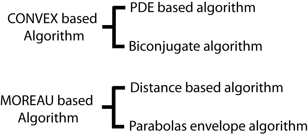
Figure 18: Different approaches for computing the Lower Compensated Convex transform $C_{\lambda}^{l}(f)$.

4.1 Convex based algorithms

Algorithms to compute convex hull such as the ones given in [35, 22] are more suitable for discrete set of points and their complexity is related to the cardinality of the set. An adaptation of these methods to our case, with the set to convexify given by the epigraph of $f+\lambda|\cdot|^{2}$, does not appear to be very effective, especially for functions defined in subsets of $\mathbb{R}^{n}$ for $n\geq 2$, compared to the methods that (directly) compute the convex envelope of a function [109, 27, 80, 42].

Of particular interest for applications to image processing, where functions involved are defined on grid of pixels, is the characterization of the convex envelope as the viscosity solution of a nonlinear obstacle problem [80]. An approximated solution is then obtained by using centered finite differences along directions defined by an associated stencil to approximate the first eigenvalue of the Hessian matrix at the grid point. A generalization of the scheme introduced in [80] in terms of the number of convex combinations of the function values at the grid points of the stencil, is briefly summarized in Algorithm 1 and described below. Given a uniform grid of points $x_{k}\in\mathbb{R}^{n}$, equally spaced with grid size $h$, denote by $S_{x_{k}}$ the $d-$point stencil of $\mathbb{R}^{n}$ with center at $x_{k}$ defined as $S_{x_{k}}=\{x_{k}+hr,|r|_{\infty}\leq 1,r\in\mathbb{Z}^{n}\}$ with $|\cdot|_{\infty}$ the $\ell^{\infty}$-norm of $r\in\mathbb{Z}^{n}$ and $d=\#(S)$, cardinality of the finite set $S$. At each grid point $x_{k}$ we compute an approximation of the convex envelope of $f$ at $x_{k}$ by an iterative scheme where each iteration step $m$ is given by

$$(\operatorname{\mathsf{co}}f)_{m}(x_{k})=\min\Big{\{}f(x_{k}),\,\sum\lambda_{i}(\operatorname{\mathsf{co}}f)_{m-1}(x_{i}):\,\,\,\sum\lambda_{i}=1,\,\lambda_{i}\geq 0,\,x_{i}\in S_{x_{k}}\Big{\}}$$

with the minimum taken between $f(x_{k})$ and only some convex combinations of $(\operatorname{\mathsf{co}}f)_{m-1}$ at the stencil grid points $x_{i}$ of $S_{x_{k}}$. It is then not difficult to show that the scheme is monotone, thus convergent. However, there is no estimate of the rate of convergence which, in actual applications, appears to be quite slow. Furthermore, results are biased by the type of underlying stencil.

1:  Set $\displaystyle m=1,\,(\operatorname{\mathsf{co}}f)_{0}=f,\,\,tol$

2:  $\displaystyle\epsilon=\|f\|_{L^{2}}$

3:  while $\displaystyle\epsilon>tol$ do

4:     $\displaystyle\forall x_{k},\quad(\operatorname{\mathsf{co}}f)_{m}(x_{k})=\min\Big{\{}f(x_{k}),\,\sum\lambda_{i}(\operatorname{\mathsf{co}}f)_{m-1}(x_{i}):\,\,\,\sum\lambda_{i}=1,\,\lambda_{i}\geq 0,\,x_{i}\in S_{x_{k}}\Big{\}}$

5:     $\displaystyle\epsilon=\|(\operatorname{\mathsf{co}}f)_{m}-(\operatorname{\mathsf{co}}f)_{m-1}\|_{L^{2}}$

6:     $m\leftarrow m+1$

7:  end while

Algorithm 1 Computation of the convex envelope of $f$ according to [80]

Based on the characterization of the convex envelope of $f$ in terms of the biconjugate $(f^{\ast})^{\ast}$ of $f$ [23, 58, 88], where $f^{\ast}$ is the Legendre-Fenchel transform of $f$, we can approximate the convex envelope by computing twice the discrete Legendre-Fenchel transform. We can thus improve speed efficiency with respect to a brute force algorithm, which computes $(f^{\ast})^{\ast}$ with complexity $O(N^{2})$ with $N$ the number of grid points, if we have an efficient scheme to compute the discrete Legendre-Fenchel transform of a function. For functions $f:X\to\mathbb{R}$ defined on cartesian sets of the type $X=\prod_{i=1}^{n}X_{i}$ with $X_{i}$ intervals of $\mathbb{R}$, $i=1,\ldots,n$, the Legendre-Fenchel transform of $f$ can be reduced to the iterate evaluation of the Legendre-Fenchel transform of functions dependent only on one varable as follows

$$\begin{split}(\xi_{1},\xi_{2},\ldots,\xi_{n})&\in\mathbb{R}^{n}\to f^{\ast}(\xi_{1},\ldots,\xi_{n})=\sup_{x\in X}\,\{\xi\cdot x-f(x)\}\\[6.45831pt] &=\sup_{x_{1},\ldots,x_{n-1}\in\prod_{i=1}^{n-1}X_{i}}\,\Big{\{}x_{1}\xi_{1}+\ldots+x_{n-1}\xi_{n-1}-\sup_{x_{n}\in X_{n}}\{x_{n}\xi_{n}-f(x_{1},\ldots,x_{n-1},x_{n})\}\Big{\}}\,.\end{split}$$ (4.1)

As a result, one can improve the complexity of the computation of $f^{\ast}$ if one has an efficient scheme to compute the Legendre-Fenchel transform of functions of only one variable. For instance, the algorithm described in [70, 57], which exploits an idea of [26] and improves the implementation of [43], computes the discrete Legendre-Fenchel transform in linear time, that is, with complexity $O(N)$. If $g_{h}$ denote the grid values of a function of one variable, the key idea of [26, 43] is to compute $(g_{h})^{\ast}$ as approximation of $g^{\ast}$ using the following result

$$(g_{h})^{\ast}(\xi)=\left(\operatorname{\mathsf{co}}[\Pi f_{h}]\right)^{\ast}(\xi)\,,\quad\quad\xi\in\mathbb{R}$$ (4.2)

where $\Pi g_{h}$ denotes the continuous piecewise affine interpolation of the grid values $g_{h}$. Therefore by applying an algorithm with linear complexity, for instance the beneath-beyond algorithm [86], to compute the convex envelope $\operatorname{\mathsf{co}}[\Pi g_{h}]$, followed by the use of analytical expressions for the Legendre-Fenchel transform of a convex piecewise affine function yields an efficient method to compute $(g_{h})^{\ast}$ [70]. For functions defined in a bounded domain, In [70] it was recommended to increment the size of the domain for a better precision of the computation of the Legendre-Fenchel transform. The work [57] avoids this by elaborating the exact expression of the Legendre-Fenchel transform of a convex piecewise affine function defined in a bounded domain which is equal to infinity in $\mathbb{R}\setminus X$ or it has an affine variation. In this manner, they can avoid bounday effects. For ease of reference, we report next the analytical expression of $g^{\ast}$ in the case where $g:\mathbb{R}\to\overline{}\mathbb{R}$ is convex piecewise affine. Without loss of generality, let $x_{1}<\ldots<x_{N}$ be a grid of points of $\mathbb{R}$, $c_{1}<\ldots<c_{N}$ and assume $g:\mathbb{R}\to\overline{}\mathbb{R}$ to be defined as follows:

$$g:x\in\mathbb{R}\to\left\{\begin{array}[]{ll}\displaystyle+\infty&\displaystyle\text{if }x\leq x_{1}\\[6.45831pt] \displaystyle g_{i}+c_{i}(x_{i}-x)&\displaystyle\text{if }x_{i}\leq x\leq x_{i+1},\quad i=1,\ldots,N-1\\[6.45831pt] \displaystyle g_{N}+c_{N}(x_{N}-x)&\displaystyle\text{if }x\geq x_{N}\end{array}\right.$$ (4.3)

where $g_{i}=g(x_{i})$ and $c_{i}$, for $i=1,\ldots,N$, represent the slopes of each affine piece of $g$. It is not difficult to verify that the analytical expression of $g^{\ast}$ is given by [57]

$$g^{\ast}:\xi\in\mathbb{R}\to\left\{\begin{array}[]{ll}\displaystyle x_{1}\xi-g_{1}&\displaystyle\text{if }\xi\leq c_{1}\\[6.45831pt] \displaystyle x_{i+1}\xi-g_{i+1}&\displaystyle\text{if }c_{i}\leq\xi\leq c_{i+1},\quad i=1,\ldots,N-2\\[6.45831pt] \displaystyle+\infty&\displaystyle\text{if }\xi\geq c_{N}\,.\end{array}\right.$$ (4.4)

Once we know $g^{\ast}$, using the decomposition (4.1), we can compute $f^{\ast}$ and thus the biconjugate $f^{\ast\ast}$.

4.2 A Moreau envelope based algorithm

The computation of the Moreau envelope is an established task in the field of computational convex analysis [72] that has been tackled by various different approaches aimed at reducing the quadratic complexity of a direct brute force implementation of the transform. Such reduction is achieved, one way or another, by a dimensional reduction. The fundamental idea of the scheme presented in [124], for instance, is the generalization of the Euclidean distance transform of binary images, by replacing the binary image by an arbitrary function on a grid. The decomposition of the structuring element which yields the exact Euclidean distance transform [99] into basic ones, leads to a simple and fast algorithm where the discrete lower Moreau envelope can be computed by a sequence of local operations, using one-dimensional neighborhoods. Unless otherwise stated, in the following, $i,\,j,\,k,\,r,\,s,\,p,\,q\in\mathbb{Z}$ denote integers whereas $m,\,n\in\mathbb{N}$ are non-negative integers. Given $n\geq 1$, we introduce grid of points of the space $\mathbb{R}^{n}$ with regular spacing $h>0$ denoted by $x_{k}\in\mathbb{R}^{n}$, $k\in\mathbb{Z}$ and define the discrete lower Moreau envelope at $x_{k}\in\mathbb{R}^{n}$ as

$$M_{\lambda}^{h}(f)(x_{k})=\inf\{f(x_{k}+rh)+\lambda h^{2}|r|^{2},\;r\in\mathbb{Z}^{n}\}\,.$$ (4.5)

By taking the infimum in (4.5) over a finite number $m\geq 1$ of directions, we obtain the $m-$th approximation of the discrete Moreau lower envelope $M_{\lambda}^{h}(f)(x_{k})$ which can be evaluated by taking the values $f_{m}(x_{k})$ given by Algorithm 2. For the convergence analysis and converegence rate we refer to [124] where it is shown that the scheme has a linear convergence rate with respect to $h$.

1:  Set $\displaystyle i=1,\,m\in\mathbb{N}$

2:  $\displaystyle\forall x_{k},\,f_{0}(x_{k})=f(x_{k})$

3:  while $\displaystyle i<m$ do

4:     $\displaystyle\tau_{i}=2i-1$

5:     $\displaystyle f_{i}(x_{k})=\min\{f_{i-1}(x_{k}+rh)+\lambda h^{2}|r|^{2}\tau_{i}:\,r\in\mathbb{Z}^{n},\,|r|_{\infty}\leq 1\}$

6:     $i\leftarrow i+1$

7:  end while

Algorithm 2 Computation of $f_{m}(x_{k})$ at the points $x_{k}$ of the grid of $\mathbb{R}^{n}$ of size $h$ for given $m\geq 1$.

Likewise the computation of the Legendre-Fenchel transform, in the scheme proposed by [49], the authors apply the dimensional reduction directly to the computation of the Moreau envelope which is factored by $n$ one dimensional Moreau envelope. For instance, in the case of $n=2$, let $\Omega=X\times Y$, with $X,Y\subset\mathbb{R}$, and $(\xi_{1},\xi_{2})\in\Omega=X\times Y$, for any $x=(x_{1},x_{2})\in\mathbb{R}^{2}$, we have

$$\begin{split}M_{\lambda}(f)(x_{1},x_{2})&=\inf_{(\xi_{1},\xi_{2})\in\Omega}\,\{\lambda|(x_{1},x_{2})-(\xi_{1},\xi_{2})|^{2}+f(\xi_{1},\xi_{2})\}\\[6.45831pt] &=\inf_{\xi_{1}\in X}\,\Big{\{}\lambda|x_{1}-\xi_{1}|^{2}+\inf_{\xi_{2}\in Y}\,\{\lambda|x_{2}-\xi_{2}|^{2}+f(\xi_{1},\xi_{2})\}\Big{\}}\,.\end{split}$$ (4.6)

For the computation of $M_{\lambda}(f)$ with $f$ function of one variable, if we denote by $\mathcal{F}$ the family of parabolas with given curvature $\lambda$ of the following type

$$\mathbcal{p}_{q}:\,x\in\mathbb{R}\,\to\,\mathbcal{p}_{q}(x)=\lambda|x-q|^{2}+f(q)\,,$$

parameterized by $q\in\Omega\subset\mathbb{R}$, we have that

$$M_{\lambda}(f)(x)=\inf\,\{\mathbcal{p}_{q}(x):\,\,\mathbcal{p}_{q}\in\mathcal{F}\}\,,$$ (4.7)

that is, the Moreau envelope of a function of one variable is reduced to the computation of the envelope of parabolas of given curvature $\lambda$. The computation of such envelope is realised by [49] in two steps. In the first one, they compute the envelope by adding the parabolas one at time which is done in linear time, and comparing each parabola to the parabolas that realise the envelope, which is done in constant time, whereas in the second step they compute the value of the envelope at the given point $x\in\mathbb{R}$. The key points of the scheme result from two observations. The first one is that given any two parabolas of $\mathcal{F}$ parameterized by $q,\,r\in\Omega$, their interesection occurs ony at one point with coordinate

$$x_{s}=\frac{(f(q)-f(r))+\lambda(q^{2}-r^{2})}{2\lambda(q-r)}\,,$$

whereas the second one regards the relation between the parabolas so that if $q<r$, then $\mathbcal{p}_{q}(x)\leq\mathbcal{p}_{r}(x)$ for $x<x_{s}$ and $\mathbcal{p}_{q}(x)\geq\mathbcal{p}_{r}(x)$ for $x>x_{s}$. This scheme allows the evaluation of $M_{\lambda}(f)(x)$ for any $x\in\mathbb{R}^{n}$ even if $f$ is defined only on a bounded open set $\Omega$, without any consideration on how to extend $f$ on $\mathbb{R}^{n}\setminus\Omega$. We will refer next to this scheme as the parabola envelope scheme.

By using the link between the Moreau envelope and the Legendre-Fenchel transform given by [90, 71]

$$M_{\lambda}(f)(x)=\lambda|x|^{2}-2\lambda\left(\frac{f}{2\lambda}+\frac{|\cdot|^{2}}{2}\right)^{\ast}(x)\,,$$ (4.8)

it is possible to design another scheme to calculate the Moreau envelope by computing the Legendre-Fenchel transform of the augmented function that appears in (4.8) [71]. In this case, however, special considerations must be taken about the primary domain, where the Moreau envelope is defined, and the dual domain, which is the one where the Legendre-Fenchel transform is defined.

5 Numerical Examples

In this section we present some illustrative numerical examples of implementation of the transforms introduced in Section 3. We preceed this discussion by the computation of a two-dimensional prototype example with analytical expression of $C_{\lambda}^{u}(\chi_{K})$ which we use to select the most suitable numerical scheme out of those described in Section 4 for the computation of the compensated convex transforms.

5.1 Prototype Example: Upper transform of a singleton set of $\mathbb{R}^{2}$

Given the singleton set $K=\{0\}\subset\mathbb{R}^{2}$, the analytical expression of $C_{\lambda}^{u}(\chi_{K})$ established in [123, Example 1.2] is given by

$$C_{\lambda}^{u}(\chi_{K})(x)=\left\{\begin{array}[]{ll}\displaystyle 0\,,&\displaystyle\text{if }|x|>1/\sqrt{\lambda}\,,\\[6.45831pt] \displaystyle\lambda(1/\sqrt{\lambda}-|x|)^{2}\,,&\displaystyle\text{if }|x|\leq 1/\sqrt{\lambda}\,.\end{array}\right.$$ (5.1)

We compute then $C_{\lambda}^{u}(\chi_{K})$ by applying the convex based algorithms, i.e. Algorithm 1 [80] and the biconjugate based scheme (shorted as $BS$ hereafter) [70, 57], and the Moreau based algorithms, i.e. Algorithm 2 and the parabola envelope scheme (shorted as $PES$ hereafter)[49]. To compare the accuracy of the schemes, we will consider: $(i)$ the Hausdorff distance between the support of the exact and the computed upper transform,

$$e_{\mathcal{H}}=\mathrm{dist}_{\mathcal{H}}\,\left(\overline{B}(0;1/\sqrt{\lambda}),\,\mathsf{sprt}\left(C_{\lambda}^{u,h}(\chi_{K})\right)\right)$$

with $C_{\lambda}^{u,h}(\chi_{K})$ the computed upper compensated transform; $(ii)$ the relative $L^{\infty}$ error norm given by

$$e_{L^{\infty}}=\frac{\max_{x\in\mathbb{R}^{2}}|C_{\lambda}^{u,h}(\chi_{K})(x)-C_{\lambda}^{u}(\chi_{K})(x)|}{\max_{x\in\mathbb{R}^{2}}|C_{\lambda}^{u}(\chi_{K})(x)|}$$

and $(iii)$ the execution time $t_{c}$ in seconds by a PC with processor Intel®  Core™  i7-4510U CPU@2.00 GHz and 8GB of memory RAM.

$\begin{array}[]{cccc}\includegraphics[width=103.28407pt]{SprtUpTrSingletonEXC.jpg}&\includegraphics[width=103.28407pt]{SprtUpTrSingletonOBE.jpg}&\includegraphics[width=103.28407pt]{SprtUpTrSingletonBIChd0_001.jpg}&\includegraphics[width=103.28407pt]{SprtUpTrSingletonMOR.jpg}\\[6.45831pt] (a)&(b)&(c)&(d)\end{array}$

Figure 19: Supports of the exact and computed upper compensated transform of the characteristic function of a singleton set of $\mathbb{R}^{2}$ by the different numerical schemes. $(a)$ Exact support given by $\overline{B}(0;1/\sqrt{\lambda})$ for $\lambda=0.01$; $(b)$ Support of $C_{\lambda}^{u,h}(\chi_{K})$ computed by Algorithm 1 [80]; $(c)$ Support of $C_{\lambda}^{u,h}(\chi_{K})$ computed by the biconjugate based scheme [70, 57] for $h_{d}=0.001$; $(d)$ Support of $C_{\lambda}^{u,h}(\chi_{K})$ computed by Algorithm 2 [124] which coincides with the one computed using the parabola envelope scheme [49].

Figure 19 displays the support of $C_{\lambda}^{u}(\chi_{K})$ given by $\overline{B}(0;1/\sqrt{\lambda})$ and of $C_{\lambda}^{u,h}(\chi_{K})$ computed by the numerical schemes mentioned above. Algorithm 2 and the parabola envelope algorithm yield the same results, thus Figure 19 displays the support as computed by only one of the two schemes. In this case we observe that the support coincides with the exact one. This does not happen for the support computed by the other two schemes. The application of Algorithm 1 evidences the bias of the scheme with the underlying stencil whereas by applying the biconjugate based scheme we note some small error all over the domain. The spread of this error depends on the dual mesh grid size $h_{d}$. Table 1 reports the values of $t_{c}$, $e_{L^{\infty}}$ and $d_{\mathcal{H}}$ for the different schemes. For the biconjugate based scheme, we have different results according to the parameter $h_{d}$ that controls the uniform discretization of the dual mesh. The value $h_{d}=1$ means that we are considering the same grid size as the grid of the input function $\chi_{K}$ whereas lower values for $h_{d}$ means that we are computing on a finer dual mesh compared to the primal one. The results given in Table 1 show that in terms of the values of $C_{\lambda}^{u}(\chi_{K})$ the biconjugate based scheme is the one that produces the best results (compare the values of $e_{L^{\infty}}$), but this occurs at the fraction of cost of reducing $h_{d}$ which means to increase the number of the dual grid nodes and consequently the computational time. The issue of the choice of the dual grid on the accuracy of the computation of the convex envelope by the conjugate has been also tackled and recognized in [42]. However, as already pointed out in the analysis of Figure 19, the support of $C_{\lambda}^{u,h}(\chi_{K})$ computed by the biconjugate scheme is the one to yield the worst value for $e_{\mathcal{H}}$.

$t_{c}$ $e_{L^{\infty}}$ $e_{\mathcal{H}}$ Convex based schemes Algorithm 1 $1.9791$ $0.0390$ $1.7321$ biconjugate scheme $h_{d}=1$ $0.1575$ $48$ $9.4999$ $h_{d}=0.1$ $0.2157$ $0.2400$ $9$ $h_{d}=0.01$ $0.5935$ $0.0142$ $7.6158$ $h_{d}=0.001$ $16.6603$ $0.0032$ $7.5498$ Moreau based schemes Algorithm 2 $0.1246$ $0.0249$ $0$ PE scheme $0.2553$ $0.0249$ $0$

Table 1: Comparison between the different numerical schemes for the computation of $C_{\lambda}^{u}(\chi_{K})$ for $\lambda=0.01$. The symbol $h_{d}$ refers to the dual mesh size of the scheme that computes the convex envelope via the biconjugate.

5.2 Intersection of Sampled Smooth Manifolds

In the following numerical experiments we verify the effectiveness of the filter $I_{\lambda}(\cdot;\,K)$ introduced in Section 3.3 and its Hausdorff stability property. We will consider both $2d-$ and $3d-$geometries. The geometry is digitized and input as an image, but also other computer representations of the geometry can clearly be handled. This depends finally on the representation of the input geometry for the numerical scheme that is used to compute the compensated transforms. Figure 20 displays a road network extract from a map of teh city of London, and represents a set of $2d$ curves which intersect to each other in different manner. The Figure shows the position of the local maxima of $I_{\lambda}(\cdot;\,K)$ which are seen to coincide with all the crossing and turning points of the given curves. We also have some false positive due to the digitization of the road network.

$\begin{array}[]{ccc}\includegraphics[width=154.9261pt]{map_roadnetwork_ma.png}&\includegraphics[width=154.9261pt]{map_roadnetwork_manetworkTPLmbd10THR110.png}&\includegraphics[width=154.9261pt]{map_roadnetwork_maTPLmbd10THR110.png}\\ (a)&(b)&(c)\end{array}$

Figure 20: $(a)$ Medial axis of the road network; $(b)$ Location of the intersection points; $(c)$ Map of the road network and location of the intersection points shown in $(b)$.

Figure 21 displays the results of the application of the filter $I_{\lambda}(\cdot;\,K)$ to $3d$ geometries represented by point clouds. Figure 21$(a)$ displays the Plücker’s conoid of parametric equation

$$x=v\cos u,\quad y=v\,\sin u,\quad z=sin4u\quad\text{for }u\in[0,\,2\pi[,\,\,v\in[-1,\,1]\,,$$

with the location of its singular lines and the parts of surface with higher curvature. Figure 21$(b)$ depicts the intersections between manifolds of different dimensions, namely, in the Figure, we have the Whitney umbrella of the implicit equation $x^{2}=y^{2}z$, a cylinder and an helix, with the location of their mutual intersections and also of where the Whitney surface intersects itself; finally, Figure 21$(c)$ displays the intersection between a cylinder, planes and an helix.

$\begin{array}[]{ccc}\includegraphics[width=140.84256pt]{plucker_vtk_cloud_tp.png}&\includegraphics[width=154.9261pt]{whitney_vtk_tp.png}&\includegraphics[width=154.9261pt]{PlanHelCyl_tp_view1.png}\\ (a)&(b)&(c)\end{array}$

Figure 21: $(a)$ Plücker surface with identification of its singular lines and surface parts of higher curvaturs; $(b)$ Intersections of the Whitney surface of equation $x^{2}=y^{2}z$ with an helix and a cylinder; $(c)$ Intersections of planes with a cylinder and an helix.

The intersection of the line with the plane for the geometry shown in Figure 21 is weaker than the geometric singularities of the surfaces. With this meaning, the values of the local maxima of $I_{\lambda}(\cdot;\,K)$ determine a scale between the different type of intersections present in the manifold $K$ and represents the multiscale nature of the filter $I_{\lambda}(\cdot;\,K)$.

Finally, the numerical experiments displayed in Figure 22 refer to critical conditions that are not directly covered by the theoretical results we have obtained. Figure 22$(a)$ shows the result of the application of $I_{\lambda}(\cdot;\,K)$ to a sphere and a cylinder that are ‘almost’ tangentially intersecting each other, whereas Figure 22$(b)$ illustrates the results of the application of the filter to detect the intersection between loosely sampled piecewise affine functions, a plane and a line.

$\begin{array}[]{cc}\includegraphics[width=211.26027pt]{CylSphTang_vtk_tp.png}&\includegraphics[width=211.26027pt]{PrPlLi-40-mrkGeoFullGEO1.png}\\ (a)&(b)\end{array}$

Figure 22: $(a)$ Tangential intersection of a sampled sphere and cylinder which are ‘almost’ tangentially intersected, and indication of the intersection marker. $(b)$ Intersection markers for the intersection among loosely sampled piecewise affine surfaces of equation $||10x-75|-|10y-75|+|10z-75|-45|$=0, the circle of equation $(10x-75)^{2}+(10z-75)^{2}\leq 45^{2}$ on the plane of equation $y=75$ and the line of equation $x=75,z=75$.

5.3 Approximation Transform

We report here on applications of the average approximation compensated convex transform developed in [119, 121] to three class of problems. These include $(i)$ surface reconstruction from real world data using level lines and single points; $(ii)$ Salt & Pepper noise restoration and $(iii)$ image inpainting.

5.3.1 Level set reconstruction

We consider here the problem of producing a Digital Elevation Map from a sample of the the NASA SRTM global digital elevation model of Earth land. The data provided by the National Elevation Dataset [51] contain geographical coordinates (latitude, longitude and elevation) of points sampled at one arc-second intervals in latitude and longitude. For our experiments, we choose the region defined by the coordinates $[\mathrm{N}\,40^{\circ}23^{\prime}25^{\prime\prime},\,\mathrm{N}\,40^{\circ}27^{\prime}37^{\prime\prime}]\times[\mathrm{E}\,14^{\circ}47^{\prime}25^{\prime\prime},\,\mathrm{E}\,14^{\circ}51^{\prime}37^{\prime\prime}]$ extracted from the SRTM1 cell $N40E014.hgt$ [103]. Such region consists of an area with extension $7.413\,\mathrm{km}\times 5.844\,\mathrm{km}$ and height varying between $115\,\mathrm{m}$ and $1282\,\mathrm{m}$, with variegated topography features. In the digitization by the US Geological Survey, each pixel represents a $30\,\mathrm{m}\times 30\,\mathrm{m}$ patch. Figure 23$(a)$ displays the elevation model from the SRTM1 data which we refer in the following to as the ground truth model. We will take a sample $f_{K}$ of such data, make the reconstruction using the $A_{\lambda}^{M}(f_{K})$ computed with Algorithm 1 and the AMLE interpolant [7, 33] using the MatLab®  code described in [83], and compare them with the ground truth model.

$\begin{array}[]{ccc}\includegraphics[width=234.73523pt]{vesuvioaoGTModel.png}&\includegraphics[width=117.36761pt]{vesuvioaoTrueBndCntrLin21Per14.png}&\includegraphics[width=117.36761pt]{vesuvioaoTrueBndSprsDataPer7.png}\\ (a)&(b)&(c)\end{array}$

Figure 23: Reconstruction of real-world digital elevation maps. $(a)$ Ground truth model from USGS-STRM1 data relative to the area with geographical coordinates; $[\mathrm{N}\,40^{\circ}23^{\prime}25^{\prime\prime},\,\mathrm{N}\,40^{\circ}27^{\prime}37^{\prime\prime}]\times[\mathrm{E}\,14^{\circ}47^{\prime}25^{\prime\prime},\,\mathrm{E}\,14^{\circ}51^{\prime}37^{\prime\prime}]$. $(b)$ Sample set $K_{1}$ formed by only level lines at regular height interval of $58.35\,\mathrm{m}$. The set $K_{1}$ contains $14\%$ of the ground truth points. $(c)$ Sample set $K_{2}$ formed by taking randomly $30\%$ of the points belonging to the level lines of the set $K_{1}$ and scattered points corresponding to $5\%$ density. The sample set $K_{2}$ contains $7\%$ of the ground truth points.

In the numerical experiments, we consider two sample data, characterized by different data density and typo of information. The first, which we refer to as sample set $K_{1}$, consists only of level lines at regular height interval of $658.35\,\mathrm{m}$ and contains the $14\%$ of the ground truth real digital data. The second sample set, denoted by $K_{2}$, has been formed by taking randomly the $30\%$ of the points belonging to the level lines of the set $K_{1}$ and scattered points corresponding to $5\%$ density so that the sample set $K_{2}$ amounts to about $7\%$ of the ground truth points. The two sample sets $K_{1}$ and $K_{2}$ are shown in Figure 23$(b)$ and Figure 23$(c)$, respectively.

$\begin{array}[]{cc}\includegraphics[width=234.73523pt]{vesuvioaoTrueBndCntrLin21Per14Lambda2000GraphOBE.png}&\includegraphics[width=234.73523pt]{vesuvioaoTrueBndSprsDataPer7Lambda2000GraphOBE.png}\\ (a)&(b)\\ \includegraphics[width=117.36761pt]{vesuvioaoTrueBndCntrLin21Per14Lambda2000IsolinesColOBE.png}&\includegraphics[width=117.36761pt]{vesuvioaoTrueBndSprsDataPer7Lambda2000IsolinesColOBE.png}\\ (c)&(d)\end{array}$

Figure 24: Reconstruction of real-world digital elevation maps. $(a)$ Graph of $A_{\lambda}^{M}(f_{K})$ for sample set $K_{1}$. Relative $L^{2}$-Errors: $\epsilon=0.0118$, $\epsilon_{K}=0$. Parameters: $\lambda=2\cdot 10^{3}$, $M=1\cdot 10^{6}$. Total number of iterations: $3818$. $(b)$ Graph of $A_{\lambda}^{M}(f_{K})$ for sample set $K_{2}$. Relative $L^{2}$-Errors: $\epsilon=0.0109$, $\epsilon_{K}=0$. Parameters: $\lambda=2\cdot 10^{3}$, $M=1\cdot 10^{6}$. Total number of iterations: $1662$. $(c)$ Isolines of $A_{\lambda}^{M}(f_{K})$ from sample set $K_{1}$ at regular heights of $58.35\,\mathrm{m}$. $(d)$ Isolines of $A_{\lambda}^{M}(f_{K})$ from sample set $K_{2}$ at regular heights of $58.35\,\mathrm{m}$.

$\begin{array}[]{cc}\includegraphics[width=234.73523pt]{vesuvioaoTrueBndCntrLin21Per14GraphAMLE.png}&\includegraphics[width=234.73523pt]{vesuvioaoTrueBndSprsDataPer7GraphAMLE.png}\\ (a)&(b)\\ \includegraphics[width=117.36761pt]{vesuvioaoTrueBndCntrLin21Per14IsolinesColAMLE.png}&\includegraphics[width=117.36761pt]{vesuvioaoTrueBndSprsDataPer7IsolinesColAMLE.png}\\ (c)&(d)\end{array}$

Figure 25: Reconstruction of real-world digital elevation maps. $(a)$ Graph of the AMLE Interpolant from set $K_{1}$. Relative $L^{2}$-Error: $\epsilon=0.0410$, $\epsilon_{K}=0.0110$. Total number of iterations: $11542$. $(b)$ Graph of the AMLE Interpolant from set $K_{2}$. Relative $L^{2}$-Error: $\epsilon=0.02863$, $\epsilon_{K}=0.0109$. Total number of iterations: $12457$. $(c)$ Isolines of the AMLE Interpolant from sample set $K_{1}$ at regular heights of $58.35\,\mathrm{m}$. $(d)$ Isolines of the AMLE Interpolant from sample set $K_{2}$ at regular heights of $58.35\,\mathrm{m}$.

The graph of the $A_{\lambda}^{M}(f_{K})$ interpolant and of the $AMLE$ interpolant for the two sample sets along with the respective isolines at equally spaced heighs equal to $58.35\,\mathrm{m}$, are displayed in Figure 24 and Figure 25, respectively, whereas Table 2 contains the values of the relative $L^{2}$-error $\epsilon$ on $\Omega$ and $\epsilon_{K}$ on the sample set $K$ between such interpolants and the ground truth model, given by, respectively,

$$\epsilon=\frac{\|f-A_{\lambda}^{M}(f_{K})\|_{L^{2}(\Omega)}}{\|f\|_{L^{2}(\Omega)}}\quad\text{and}\quad\epsilon_{K}=\frac{\|f_{K}-A_{\lambda}^{M}(f_{K})\|_{L^{2}(K)}}{\|f_{K}\|_{L^{2}(K)}}\,,$$ (5.2)

where $f$ is the ground truth model and $A_{\lambda}^{M}(f_{K})$ is the average approximation of the sample $f_{K}$ of $f$ over $K$. We observe that while $A_{\lambda}^{M}(f_{K})$ yields an exact interpolation of $f_{K}$ over $\Omega$, this is not the case for the AMLE approximation.

$\epsilon$ $\epsilon_{K}$ Sample set $A_{\lambda}^{M}(f_{K})$ AMLE $A_{\lambda}^{M}(f_{K})$ AMLE $K_{1}$ $0.0118$ $0.0410$ $0$ $0.0110$ $K_{2}$ $0.0109$ $0.0286$ $0$ $0.0109$

Table 2: Relative $L^{2}$-error for the DEM Reconstruction from the two sample sets using the $A_{\lambda}^{M}(f_{K})$ and the AMLE interpolant. The realization of $\epsilon_{K}=0$ for $A_{\lambda}^{M}(f_{K})$ says that $A_{\lambda}^{M}(f_{K})$ yields an exact interpolation of $f_{K}$ over $\Omega$, unlike the AMLE approximation.

Though both reconstructions are comparable visually to the ground truth model, a closer inspection of the pictures show that the reconstruction from the synthetic data, the AMLE interpolant does not reconstruct correctly the mountains peaks, which appear to be smoothed, and introduce artificial ridges along the slopes of the mountains. In contrast, the $A_{\lambda}^{M}(f_{K})$ interpolant appears to better for capturing features of the ground truth model. Finally, we also note that though the sample set $K_{1}$ contains a number of ground truth points higher than the sample set $K_{2}$, the reconstruction from $K_{2}$ appears to be better than the one obtained from $K_{1}$. This behaviour was found for both interpolations, though it is more notable in the case of the $A_{\lambda}^{M}(f_{K})$ interpolant. By taking scattered data, we are able to get a better characterization of irregular surfaces, compared to the one obtained from a structured representation such as provided by the level lines.

5.3.2 Salt & Pepper Noise Removal

As an application of scattered data approximation to image processing, we consider here the restoration of an image corrupted by salt & pepper noise. This is an impulse type noise that is caused, for instance, by malfunctioning pixels in camera sensors or faulty memory locations in hardware, so that information is lost at the faulty pixels and the corrupted pixels are set alternatively to the minumum or to the maximum value of the range of the image values. When the noise density is low, about less than $40\%$, the median filter [13] or its improved adaptive median filter [59], is quite effective for restoring the image. However, this filter loses its denoising power for higher noise density given that details and features of the original image are smeared out. In those cases, other techniques must be applied; one possibility is the two-stage TV-based method proposed in [34] which consists of applying first an adaptive median filter to identify the pixels that are likely to contain noise and construct thus a starting guess which is used in the second stage for the minimization of a functional of the form

$$F(u,y)=\Psi(u,y)+\alpha\Phi(u)$$

where $y$ denotes the noisy image, $\Psi$ is a data-fidelty term and $\Phi$ is a regularization term, with $\alpha>0$ a parameter. In the following numerical experiments, we consider the image displayed in Figure 26$(a)$ with size $512\times 512$ pixels, damaged by $70\%$ salt & pepper noise. The resulting corrupted image is displayed in Figure 26$(b)$ where on average only $78643$ pixels out of the total $262144$ pixels carry true information. The true image values represent our sample function $f_{K}$ whereas the set of the true pixels forms our sample set $K$. To assess the restoration performance we use the peak signal-to-noise ratio ($\mathrm{PSNR}$) which is expressed in the units of $\mathrm{dB}$ and, for an $8-$bit image, i.e. with values in the range $[0,\,255]$, is defined by

$$\mathrm{PSNR}=10\log_{10}\displaystyle\frac{255^{2}}{\frac{1}{mn}\sum_{i,j}|f_{i,j}-r_{i,j}|^{2}}$$ (5.3)

where $f_{i,j}$ and $r_{i,j}$ denote the pixels values of the original and restored image, respectively, and $m,\,n$ denote the size of the image $f$. In our numerical experiments, we have considered the following cases. The first one assumes the set $K$ to be given by the noise-free interior pixels of the corrupted image together with the boundary pixels of the original image. In the second case, $K$ is just the set of the noise-free pixels of the corrupted image, without any special consideration on the image boundary pixels. In analysing this second case, to reduce the boundary effects produced by the application of Algorithm 1 and Algorithm 2, we have applied our method to an enlarged image and then restricted the resulting restored image to the original domain. The enlarged image has been obtained by padding a fixed number of pixels before the first image element and after the last image element along each dimension, making mirror reflections with respect to the boundary. The values used for padding are all from the corrupted image. In our examples, we have considered two versions of enlarged images, obtained by padding the corrupted image with 2 pixels and 10 pixels, respectively. Table 3, Table 4 and Table 5 compare the values of the $\mathrm{PSNR}$ of the restored images by our method and the TV-based method applied to the corrupted image with noise-free boundary and to the two versions of the enlarged images with the boundary values of the enlarged images given by the padded noisy image data. We observe that there are no important variations in the denoising result between the different methods of treating the image boundary. This is also reflected by the close value of the $\mathrm{PSNR}$ of the resulting restored images. For $70\%$ salt & pepper noise, Figure 26$(c)$ and Figure 26$(d)$ display the restored image $A_{\lambda}^{M}(f_{K})$ by Algorithm 1 and Algorithm 2, respectively, with $K$ equal to the true set that has been enlarged by two pixels, whereas Figure 26$(e)$ and Figure 26$(f)$ show the restored image by the Adaptive median Filter and the TV-based method [28, 34] using the same set $K$. Although the visual quality of the images restored from $70\%$ noise corruption is comparable between our method and the TV-based method, the $\mathrm{PSNR}$ using our method with Algorith 1 is higher than that for the TV-based method in all of the experiments reported in Table 3, Table 4 and Table 5. An additional advantage of our method is its speed. Our method does not require initialisation which is in contrast with the two-stage TV-based method, for which the initialisation, for instance, is given by the restored image using an adaptive median filter.

$\mathrm{PSNR}$ $K$ with noise-free boundary $A_{\lambda}^{M}(f)$ TV Noise Density Algorithm 1 Algorithm 2 $70\%$ ($6.426\,\mathrm{dB}$) $26.674\,\mathrm{dB}$ $26.634\,\mathrm{dB}$ $26.506\,\mathrm{dB}$ $90\%$ ($5.371\,\mathrm{dB}$) $23.117\,\mathrm{dB}$ $22.968\,\mathrm{dB}$ $22.521\,\mathrm{dB}$ $99\%$ ($4.938\,\mathrm{dB}$) $18.424\,\mathrm{dB}$ $18.357\,\mathrm{dB}$ $17.420\,\mathrm{dB}$

Table 3: Comparison of $\mathrm{PSNR}$ of the restored images by the compensated convexity based method ($A_{\lambda}^{M}(f_{K})$) by applying the Moreau based scheme (Algorithm 1) and the convex based scheme (Algorithm 2), and by the two-stage TV-based method (TV), with the set $K$ with noise–free boundary.

$\mathrm{PSNR}$ $K$ padded by two pixels $A_{\lambda}^{M}(f)$ TV Noise Density Algorithm 1 Algorithm 2 $70\%$ ($6.426\,\mathrm{dB}$) $26.642\,\mathrm{dB}$ $26.020\,\mathrm{dB}$ $26.475\,\mathrm{dB}$ $90\%$ ($5.371\,\mathrm{dB}$) $23.078\,\mathrm{dB}$ $22.654\,\mathrm{dB}$ $22.459\,\mathrm{dB}$ $99\%$ ($4.938\,\mathrm{dB}$) $18.240\,\mathrm{dB}$ $18.026\,\mathrm{dB}$ $17.314\,\mathrm{dB}$

Table 4: Comparison of $\mathrm{PSNR}$ of the restored images by the compensated convexity based method ($A_{\lambda}^{M}(f_{K})$) by applying the Moreau based scheme (Algorithm 1) and the convex based scheme (Algorithm 2), and by the two-stage TV-based method (TV), with the set $K$ padded by two pixels.

$\mathrm{PSNR}$ $K$ padded by ten pixels $A_{\lambda}^{M}(f)$ TV Noise Density Algorithm 1 Algorithm 2 $70\%$ ($6.426\,\mathrm{dB}$) $26.640\,\mathrm{dB}$ $26.020\,\mathrm{dB}$ $26.468\,\mathrm{dB}$ $90\%$ ($5.371\,\mathrm{dB}$) $23.068\,\mathrm{dB}$ $22.654\,\mathrm{dB}$ $22.446\,\mathrm{dB}$ $99\%$ ($4.938\,\mathrm{dB}$) $18.342\,\mathrm{dB}$ $18.026\,\mathrm{dB}$ $17.330\,\mathrm{dB}$

Table 5: Comparison of $\mathrm{PSNR}$ of the restored images by the compensated convexity based method ($A_{\lambda}^{M}(f_{K})$) by applying the Moreau based scheme (Algorithm 1) and the convex based scheme (Algorithm 2), and by the two-stage TV-based method (TV), with the set $K$ padded by ten pixels.

Finally, to demonstrate the performance of our method in some extreme cases of very sparse data, we consider cases of noise density equal to $90\%$ and $99\%$. Figure 27 displays the restored image by the compensated convexity based method and by the TV-based method for the case where $K$ is padded by two pixels and ten pixels for $90\%$ and $99\%$ noise level, respectively. As far as the visual quality of the restored images is concerned, and to the extent that such judgement can make sense given the high level of noise density, the inspection of Figure 27 seems to indicate that $A_{\lambda}^{M}(f_{K})$ gives a better approximation of details than the TV-based restored image. This is also reflected by the values of the $\mathrm{PSNR}$ index in the Table 3, Table 4 and Table 5.

$\begin{array}[]{cc}\includegraphics[width=164.31752pt]{PirateScl.png}&\includegraphics[width=164.31752pt]{PirateDNS0_7N1.png}\\ (a)&(b)\\ \includegraphics[width=164.31752pt]{PirateS_PDNS0_7N1Lmbd20M1e13EXT2MORLocRest.png}&\includegraphics[width=164.31752pt]{PirateS_PDNS0_7N1Lmbd20M1e13EXT2OBELocRest.png}\\ (c)&(d)\\ \includegraphics[width=164.31752pt]{PirateS_PDNS0_7N1EXT2AdaptiveMedianFilter.png}&\includegraphics[width=164.31752pt]{PirateS_PDNS0_7N1EXT2NCLocRest.png}\\ (e)&(f)\end{array}$

Figure 26: $(a)$ Original image; $(b)$ Original image covered by a salt & pepper noise density of $70\%$. $\mathrm{PSNR}=6.426\,\mathrm{dB}$; $(c)$ Restored image $A_{\lambda}^{M}(f_{K})$ by Moreau based scheme (Algorithm 2) with the set $K$ padded by two pixels. $\mathrm{PSNR}=26.020\,\mathrm{dB}$. $\lambda=20$, $M=1E13$. Total number of iterations: $21$. $(d)$ Restored image $A_{\lambda}^{M}(f_{K})$ by Convex based scheme (Algorithm 1) with the set $K$ padded by two pixels. $\mathrm{PSNR}=26.642\,\mathrm{dB}$. $\lambda=20$, $M=1E13$. Total number of iterations: $1865$. $(e)$ Restored image by the Adaptive Median filter [59] used as starting guess for the two-stage TV-based method described in [28, 34]. Window size $w=33$ pixels. $\mathrm{PSNR}=22.519\,\mathrm{dB}$. $(f)$ Restored image by the two-stage TV-based method described in [28, 34] with the set $K$ padded by two pixels. $\mathrm{PSNR}=26.475\,\mathrm{dB}$. Total number of iterations: $3853$.

$\begin{array}[]{ccc}\includegraphics[width=154.9261pt]{PirateS_PDNS0_9N1Lmbd10M1e13EXT2MORLocRest.png}&\includegraphics[width=154.9261pt]{PirateS_PDNS0_9N1Lmbd10M1e13EXT2OBELocRest.png}&\includegraphics[width=154.9261pt]{PirateS_PDNS0_9N1EXT2NCLocRest.png}\\ (a)&(b)&(c)\\ \includegraphics[width=154.9261pt]{PirateS_PDNS0_99N1Lmbd2M1e13EXT2OBELocRest.png}&\includegraphics[width=154.9261pt]{PirateS_PDNS0_99N1Lmbd2M1e13EXT2MORLocRest.png}&\includegraphics[width=154.9261pt]{PirateS_PDNS0_99N1EXT2NCLocRest.png}\\ (d)&(e)&(f)\end{array}$

Figure 27: Restoration of $90\%$ corrupted image ($\mathrm{PSNR}=5.372\,\mathrm{dB}$) with the set $K$ padded by two pixels. $(a)$ Restored image $A_{\lambda}^{M}(f_{K})$ by Moreau based scheme (Algorithm 2). $\mathrm{PSNR}=22.654\,\mathrm{dB}$. $\lambda=10$, $M=1e13$. Total number of iterations equal to $32$ $(b)$ Restored image $A_{\lambda}^{M}(f_{K})$ by Convex based scheme (Algorithm 1). $\mathrm{PSNR}=23.078\,\mathrm{dB}$. $\lambda=10$, $M=1e13$. Total number of iterations equal to $10445$ $(c)$ Restored image by the two-stage TV-based method described in [28, 34]. $\mathrm{PSNR}=22.459\,\mathrm{dB}$. Total number of iterations: $2679$.
Restoration of $99\%$ corrupted image ($\mathrm{PSNR}=4.938\,\mathrm{dB}$), with the set $K$ padded by ten pixels. $(d)$ Restored image $A_{\lambda}^{M}(f_{K})$ by Moreau based scheme (Algorithm 2). $\mathrm{PSNR}=18.026\,\mathrm{dB}$. $\lambda=2$, $M=1e13$. Total number of iterations equal to $78$ $(e)$ Restored image $A_{\lambda}^{M}(f_{K})$ by Convex based scheme (Algorithm 1). $\mathrm{PSNR}=18.342\,\mathrm{dB}$. $\lambda=2$, $M=1e13$. Total number of iterations equal to $54823$ $(f)$ Restored image by the two-stage TV-based method described in [28, 34]. $\mathrm{PSNR}=17.330\,\mathrm{dB}$. Total number of iterations: $13125$.

5.3.3 Inpainting

Inpainting is the problem where we are given an image that is damaged in some parts and we want to reconstruct the values in the damaged part on the basis of the known values of the image. This topic has attracted lot of interest especially as an application of TV related models [37, 95]. The main motvation is that functions of bounded variations provide the appropriate functional setting given that such functions are allowed to have jump discontinuities [9]. These authors usually argue that continuous functions cannot be used to model digital image related functions as functions representing images may have jumps [37], which are associated with the image features. However, from the human vision perspective, it is hard to distinguish between a jump discontinuity, where values change abruptly, and a continuous function with sharp changes within a very small transition layer. By the application of our compensated convex based average transforms we are adopting the latter point of view. A comprehensive study of this theory applied to image inpainting can be found in [119, 121] where we also establish error estimates for our inpainting method and compare with the error analysis for image inpainting discussed in [36]. We note that for the relaxed Dirichlet problem of the minimal graph [36] or of the TV model used in [36], as the boundary value of the solution does not have to agree with the original boundary value, extra jumps can be introduced along the boundary. By comparison, since our average approximation is continuous, it will not introduce such a jump discontinuity at the boundary.

$\begin{array}[]{cc}\includegraphics[width=211.26027pt]{LenaImgMask.png}&\includegraphics[width=211.26027pt]{LenaLmbd58IT73M100000OBELocRestImg.png}\\ (a)&(b)\\ \includegraphics[width=211.26027pt]{LenaAMLELocRstImg.png}&\includegraphics[width=211.26027pt]{LenaRstImgTV.png}\\ (c)&(d)\end{array}$

Figure 28: Inpainting of a text overprinted on an image: $(a)$ Input image. $(b)$ Restored image $A_{\lambda}^{M}(f_{K})$ using Algorithm 2. $\mathrm{PSNR}=39.122\,\mathrm{dB}$. Parameters: $\lambda=18$ and $M=1\cdot 10^{5}$. Total number of iterations: $19$. $(c)$ Restored image by the AMLE method described in [95, 83]. $\mathrm{PSNR}=36.406\,\mathrm{dB}$. Total number of iterations: $5247$. $(d)$ Restored image by the Split Bregman inpainting method described in [52]. $\mathrm{PSNR}=39.0712\,\mathrm{dB}$. Total number of iterations: $19$.

To assess the performance of our reconstruction compared to state-of-art inpainting methods, we consider synthetic example where we are given an image $f$ and we overprint some text on it. The problem is then removing the text overprinted on the image displayed in Figure 28$(a)$ and how close we can get to the original image $f$. If we denote by $P$ the set of pixels containing the overprinted text, and by $\Omega$ the domain of the whole image, then $K=\Omega\setminus P$ is the set of the true pixels and the inpainting problem is in fact the problem of reconstructing the image over $P$ from knowing $f_{K}$, if we denote by $f$ the original image values. we compare our method with the total variation based image inpainting method solved by the split Bregman method described in [52] and with the AMLE inpainting reported in [95]. The restored image $A_{\lambda}^{M}(f_{K})$ obtained by our compensated convexity method is displayed in Figure 28$(b)$, the restored image by the AMLE method is shown in Figure 28$(d)$ whereas 28$(c)$ presents the restored image by the the split Bregman inpainting method. All the restored images look visually quite good. However, if we use the $\mathrm{PSNR}$ as a measure of the quality of the restoration, we find that $A_{\lambda}^{M}(f_{K})$ has a value of $\mathrm{PSNR}$ equal to $39.122\,\mathrm{dB}$, the split Bregman inpainting restored image gives a value for $\mathrm{PSNR}=39.071\,\mathrm{dB}$, whereas the AMLE restored image has $\mathrm{PSNR}$ equal to $36.406\,\mathrm{dB}$. To assess how well $A_{\lambda}^{M}(f_{K})$ is able to preserve image details and not to introduce unintended effects such as image blurring and staircase effects, Figure 29 displays details of the original image and of the restored images by the three methods. Once again, the good performance of $A_{\lambda}^{M}(f_{K})$ can be appreciated visually.

$\begin{array}[]{c}\begin{array}[]{cc}\includegraphics[width=211.26027pt]{LenaImgdetail.png}&\includegraphics[width=211.26027pt]{LenaMaskImgdetail.png}\\ (a)&(b)\end{array}\\ \begin{array}[]{ccc}\includegraphics[width=154.9261pt]{LenaLmbd58M73OBELocRstImgdetail.png}&\includegraphics[width=154.9261pt]{LenaRstImgTVdetail}&\includegraphics[width=154.9261pt]{LenaAMLERstImgdetail}\\ (c)&(d)&(e)\end{array}\end{array}$

Figure 29: Comparison of a detail of the original image with the corresponding detail of the restored images according to the compensated convexity method and the TV-based method. Lips detail of the original: image $(a)$ without and $(b)$ with overprinted text. Lips detail of the: $(c)$ restored image $A_{\lambda}^{M}(f_{K})$ using Algorithm 2; $(d)$ AMLE-based restored image; $(d)$ TV-based restored image.

We conclud ethis section with two real–world applications, where we actaully do not know the true background pciture $f$, thus the assessment of the inpainting must simply rely on the visual quality of the approximation. Figure 30 compares the results of the Average compensated approximation and of the TV-based approximation in the case of the restoration of an image containing a scratch, whereas Figure LABEL:Fig.NumEx7.3d refers to the removal of an unwanted thin object from a picture. For both the examples, the two approximations yield qualitatively good results.

$\begin{array}[]{cc}\includegraphics[width=211.26027pt]{Lincoln371x432.jpg}&\includegraphics[width=211.26027pt]{Lincoln371x432colMaskImg.png}\\ (a)&(b)\\ \includegraphics[width=211.26027pt]{Lincoln371x432colLmbd15M100000OBERstImg.png}&\includegraphics[width=211.26027pt]{Lincoln371x432colTVRestImgCol.png}\\ (c)&(d)\end{array}$

Figure 30: Restoration of an old image. $(a)$ Input image with the scratch. $(b)$ Input image with manual definition of the mask, given by the domain to respair. $(c)$ Restored image $A_{\lambda}^{M}(f_{K})$ with $\lambda=15$, $M=10^{6}$. $(d)$ TV-based restored image.

$\begin{array}[]{cc}\includegraphics[width=211.26027pt]{jmpgm600x722.jpg}&\includegraphics[width=211.26027pt]{jmpgm600x722VR3MaskImg.png}\\ (a)&(b)\\ \includegraphics[width=211.26027pt]{jmpgm600x722VR3Lmbd15M100000OBERstImg.png}&\includegraphics[width=211.26027pt]{jmpgm600x722VR3TVRestImgCol.png}\\ (c)&(d)\end{array}$

Figure 31: Removal of a thin object from a picture. $(a)$ Input image. $(b)$ Input image with manual definition of the mask, given by the domain to be inpainted. $(c)$ Restored image $A_{\lambda}^{M}(f_{K})$ with $\lambda=15$, $M=10^{6}$. $(d)$ TV-based restored image.

References

- [1] Aichholzer O., Aigner W., Aurenhammer F., Hackl T., Jüttler B., Rabl M., Medial axis computation for planar free-form shapes, Comput. Aided Design 41 (2009) 339–349.
- [2] Albano P., The regularity of the distance function propagates along minimizing geodesics, Nonlinear Anal. 95 (2014) 308–312.
- [3] Albano P., Cannarsa P., Structural properties of singularities of semiconcave functions, Ann. Scuola Norm. Sup. Pisa Cl. Sci. 28 (1999) 719–740.
- [4] Albano P., Cannarsa P., Nguyen K. T., Sinestrari C., Singular gradient flow of the distance function and homotopy equivalence, Math. Ann. 356 (2013) 23–43.
- [5] Alberti G., On the structure of singular sets of convex functions, Calculus of Variations and Partial Differential Equations 2 (1994) 17–27.
- [6] Alberti G., Ambrosio L., Cannarsa P., On the singularities of convex functions, Manuscripta Math. 76 (1992) 421–435.
- [7] Almansa A., Cao F., Gousseau , Rougé B., Interpolation of digital elevation models using AMLE and related methods, IEEE Trans. Geoscience and Remote Sensing 40 (2002) 314–325.
- [8] Alvarez L., Guichard F., Lions P.L., Morel J.M., Axioms and fundamental equations in image processing. Arch. Ration. Mech. Anal. 123 (1993) 199–257.
- [9] Ambrosio L., Fusco N., Pallara D., Functions of Bounded Variation and Free Discontinuity Problems, Clarendon Press, UK, 2000.
- [10] Ambrosio L., Tilli P., Topics on Analysis in Metric Spaces, Oxford Univ. Press, 2004.
- [11] Amenta N., Bern M., Surface reconstruction by Voronoi filtering, Discrete Comput. Geom. 22 (1999) 481–504.
- [12] Amenta N., Choi S., Kolluri R., The power crust, unions of balls, and the medial axis transform, Comp. Geom-Theor. Appl. 19 (2001) 127–153
- [13] Astola J., Kuosmanen P., Fundamentals of Nonlinear Digital Filtering. CRC Press, Boca Raton, 1997
- [14] Attali D., Lieutier A., Optimal reconstruction might be hard, Discrete Comput. Geom. 49 (2013) 133–156.
- [15] Attali D., Montanvert A., Computing and simplifying 2D and 3D semicontinuous skeletons of 2D and 3D shapes, Comput. Vis. Image Und. 67 (1997) 261–273.
- [16] Attouch H., Aze D., Approximations and regularizations of arbitrary functions in Hilbert spaces by the Lasry-Lions methods, Anal. Non-Lin. H. Poincaré Inst. 10 (1993) 289-312.
- [17] Aubert G., Kornprobst P., Mathematical Problems in Image Processing. Partial Differential Equations and the Calculus of Variations. Springer Berlin 2006
- [18] Aussel D., Daniilidis A., Thibault L., Subsmooth sets: functional characterizations and related concepts, Trans. Am. Math. Soc. 357 (2005) 1275–1301.
- [19] Ball J., The calculus of variations and materials science Quarterly of Applied Mathematics LVI (1998) 719–740.
- [20] Ball J. M., James R. D., Fine phase mixtures as minimizers of energy, Arch. Rational Mech. Anal. 100 (1987) 13–52.
- [21] Ball J. M., James R. D., Proposed experimental tests of a theory of fine microstructures and the two-well problem, Phil. Royal Soc. Lond. A 338 (1992) 389–450.
- [22] Barber, C. B., Dobkin, D. P., Huhdanpaa, H., The quickhull algorithm for convex hulls. ACM Transactions on Mathematical Software 22 (1996) 469–483.
- [23] Bauschke, H. H., Combettes, P. L., Convex Analysis and Monotone Operator Theory in Hilbert Spaces Springer Verlag, Berlin, 2nd ed., 2017.
- [24] Blum H., A transformation for extracting new descriptors of shape, Prop. Symp. Models for the Perception of Speech and Visual Form (W. W. Dunn ed.), MIT Press (1967) 362–380.
- [25] Boissonnat J.D., Cazals F., Smooth surface reconstruction via natural neighbor interpolation of distance functions, ACM Symposium on Computational Geometry (2000) 223–232.
- [26] Brenier Y., Un algorithme rapide pour le calcul de transformées de Legendre-Fenchel discrétes. C.R. Acad. Sci. Paris Sér. I Math. 308 (1989) 587–589.
- [27] Brighi B., Chipot M., Approximated convex envelope of a function. SIAM Journal on Numerical Analysis 31 (1994) 128–148.
- [28] Cai J.-F., Chan R., Morini B., Minimization of an edge-preserving regularization functional by conjugate gradient type methods. In: Image Processing Based on Partial Differential Equations, Tai X.-C., Lie K.-A., Chan T. F., Osher S., Eds., Springer (2005) 109–122.
- [29] Calabi L., Hartnett W. E., Shape recognition, prairie fires, convex deficiencies and skeletons, The American Mathematical Monthly 75 (1968) 335–342.
- [30] Cannarsa P., Peirone R., Unbounded components of the singular set of the distance function in , Transactions of the American Mathematical Society 353 (2001) 4567–4581.
- [31] Cannarsa P., Sinestrari C., Semiconcave Functions, Hamilton-Jacobi Equations and Optimal Control, Birkhäuser, Boston, 2004.
- [32] Carlsson M., On convex envelopes and regularization of non-convex functionals without moving global minima. Journal of Optimization Theory and Applications 183 (2019) 66–84.
- [33] Caselles V., Morel J.-M., Sbert C., An axiomatic approach to image interpolation, IEEE Trans. Image Processing 7 (1998) 376–386.
- [34] Chan R.H., Ho C.-W., Nikolova M., Salt-and-pepper noise removal by median-type noise detectors and detail-preserving regularization. IEEE Transactions on Image Processing 14 (2005) 1479–1485.
- [35] Chan T. M., Optimal output-sensitive convex hull algorithms in two and three dimensions. Discrete and Computational Geometry 16 (1996) 361–368.
- [36] Chan T. F., Kang S. H., Error analysis for image inpainting, J. Math. Imag. Vis. 26 (2006) 85–103.
- [37] Chan T., Shen J., Image Processing and Analysis: Variational, PDE, Wavelet, and Stochastic Methods, SIAM, 2005.
- [38] Chazal F., Soufflet R., Stability and finiteness properties of medial axis and skeleton, J. Control Dyn. Sys. 10 (2004) 149–170.
- [39] Choi H. I., Choi S. W., Moon H. P., Mathematical theory of medial axis transform, Pacific J. Math. 181 (1997) 57–88.
- [40] Choi S. W., Seidel H.-P., Linear one-sided stability of MAT for weakly injective 3D domain, Comput. Aided Design 36 (2004) 95–109.
- [41] Clarke F.H., Ledyaev Yu.S., Stern R.J., Wolenski P.R., Nonsmooth Analysis and Control Theory, Springer-Verlag, New York, 1998.
- [42] Contento L., Ern A., Vermiglio R., A linear-time approximate convex envelope algorithm using the double Legendre-Fenchel transform with application to phase separation. Computational Optimization and Applications volume 60 (2015) 231–261.
- [43] Corrias L., Fast Legendre-Fenchel transform and applications to Hamilton-Jacobi equations and conservation laws. SIAM Journal on Numerical Analysis 33 (1996) 1534–1558.
- [44] Crandall M. G., Ishii H., Lions P.-L., User’s guide to visosity solutions of second order partial differential equations, Bull. Am. Math. Soc. 27 (1992) 1–67.
- [45] Dacorogna B., Direct Methods in the Calculus of Variations, Springer–Verlag, New York, 2008, 2nd Ed.
- [46] DeVore R.A., Lorentz G.G., Constructive Approximation, Springer-Verlag, Berlin, 1993.
- [47] Dey T. K., Curve and Surface Reconstruction, Cambridge University Press, 2006.
- [48] Dey T. K., Zhao W., Approximating the medial axis from the Voronoi diagram with a convergence guarantee, Algorithmica 38 (2004) 356–366.
- [49] Felzenszwalb P. F., Huttenlocher D. P., Distance transforms of sampled functions. Theory of Computing 8 (2012) 415–428.
- [50] Firoozye, N. B., Optimal use of the translation method and relaxations of variational problems. Communications on Pure and Applied Mathematics 44 (1991) 643–678.
- [51] Gesch D., Evans G., Mauck J., Hutchinson J., Carswell Jr W. J., The national map elevation, U.S. Geological Survey Fact Sheet 3053, 2009.
- [52] Getreuer P., Total variation inpainting using split Bregman. Image Processing On Line 2 (2012) 147–157.
- [53] Giusti E., Minimal Surfaces and Functions of Bounded Variation, Birkhäuser Verlag, Switzerland, 1984.
- [54] Grabovsky, Y., Bounds and extremal microstructures for two-component composites: A unified treatment based on the translation method. Proceedings of the Royal Society of London. Series A: Mathematical, Physical and Engineering Sciences, 452 (1996) 919–944.
- [55] Hare W.L., A proximal average for nonconvex functions: A proximal stability perspective. SIAM Journal on Optimization 20 (2009) 650–666.
- [56] Hartman P., On functions representable as a difference of convex functions, Pacific J. Math. 9 (1959), 707–713.
- [57] Helluy P., Mathis H., Pressure laws and fast Legendre transform. Mathematical Models and Methods in Applied Sciences 21 (2011) 745–775.
- [58] Hiriart-Urruty J.-B., Lemaréchal C., Fundamentals of Convex Analysis. Springer, 2001.
- [59] Hwang H, Haddad R.A., Adaptive median filters: New algorithms and results. IEEE Transactions on Image Processing 4 (1995) 499–502.
- [60] Jackway P. T., Morphological scale-space, IAPR International Conference on Pattern Recognition, IEEE Computer Society Press, Los Alamitos, CA (1992) 252–255.
- [61] Jackway P.T., Properties of multiscale morphological smoothing by poweroids. Pattern Recognit. Lett. 15 (1994) 135–140.
- [62] Jackway P.T., On dimensionality in multiscale morphological scale–space with elliptic poweroid structuring functions. J. Vis. Commun. Image Represent. 6 (1995) 189–195.
- [63] Jackway P.T., Deriche M., Scale–space properties of the multiscale morphological dilation–erosion. IEEE Trans. Pattern Anal. Mach. Intell. 18 (1996) 38–51
- [64] Kimmel R., Shaked D., Kiryati N., Bruckstein A., Skeletonization via distance maps and level sets, Comput. Vis. Image Und. 62 (1995) 382–391.
- [65] Koenderink J.J., The structure of images. Biol. Cybernet. 50 (1984) 363–370.
- [66] Lasry J.M., Lions P.L., A remark on regularization in Hilbert Spaces, Israel Math. J. 55 (1986) 257-266.
- [67] Lieutier A., Any open bounded subset of has the same homotopic type as its medial axis, Comput. Aided Design 36 (2004) 1029–1046.
- [68] Lindeberg T., Scale-Space Theory in Computer Vision. Kluwer, Boston, 1994.
- [69] Lindeberg T., Generalized Gaussian scale-space axiomatics comprising linear scale-space, affine scale-space and spatio-temporal scale-space. J. Math. Imaging Vis. 40 (2011) 36–81.
- [70] Lucet Y., Faster than the Fast Legendre-Transform, the linear-time Legendre Transform. Numerical Algorithms 16 (1997) 171–185.
- [71] Lucet Y., Fast Moreau envelope computation I: numerical algorithms. Numerical Algorithms 43 (2006) 235–249.
- [72] Lucet Y., What shape is your conjugate? A survey of computational convex analysis and its applications. SIAM Review 52 (2010) 505–542.
- [73] Mantegazza C., Mennucci A. C., Hamilton-Jacobi equations and distance functions on Riemannian manifolds. Appl. Math. Optim. 47 (2003) 1–25.
- [74] Maragos P., Schafer R., Morphological filters-Part I: their settheoretic analysis and relations to linear shift-invariant filters. IEEE Trans. Acoust. Speech Signal Process. 35 (1987) 1153–1169.
- [75] Matheron G., Examples of topological properties of skeletons, J. Serra (Ed), Image Analysis and Mathematical Morpholpogy, Part II, Academic Press, 1988.
- [76] Milton, G. W., On characterizing the set of possible effective tensors of composites: The variational method and the translation method. Communications on Pure and Applied Mathematics 43 (1990) 63–125
- [77] Moreau J.-J., Proximaté dualité dans un espace Hilbertien, Bull. Soc. Math. Fr. 93 (1965) 273–299.
- [78] Moreau J.-J., Fonctionnelles Convexes, Lecture Notes, Collége de France, 1966.
- [79] Okabe A., Boots B., Sugihara K., Chiu S. N., Spatial Tessellations–Concepts and Applications of Voronoi Diagrams. John Wiley & Sons, Second Edition, 2000.
- [80] Oberman A. M., Computing the convex envelope using a nonlinear partial differential equation. Math. Models Methods Appl. Sci. 18 (2008) 759–780.
- [81] Ogniewicz R. L., Kübler O., Hierarchic Voronoi skeletons, Pattern Recogn. 28 (1995) 343–359.
- [82] Parikh N., Boyd S., Proximal algorithms, Foundations and Trends in Optimization 1 (2013) 123–231.
- [83] Parisotto S., Schönlieb B.-C., MATLAB Codes for the Image Inpainting Problem, GitHub repository, MATLAB Central File Exchange, September, 2016.
- [84] Parisotto S., Lellmann J., Masnou S., Schönlieb C.-B., Higher-order total directional variation. Part I: Imaging applications. Available at https://arxiv.org/abs/1812.05023.
- [85] Patrikalakis N. M., Maekawa T., Shape Interrogation for Computer Aided Design and Manufacturing, Springer, Heidelberg, 2002.
- [86] Preparata F. P., Shamos M., Computational Geometry. An Introduction, Springer Verlag, Berlin, 1985.
- [87] Reshetnyak Y. G., On a generalization of convex surfaces, Mat. Sbornik 40 (1956) 381–398.
- [88] Rockafellar R. T., Convex Analysis, Princeton Univ. Press, New Jersey, 1970.
- [89] Rockafellar R. T., Clarke’s tangent cones and boundaries of closed sets in , Nonlinear Analysis: Theory, Methods & Applications 3 (1979) 145–154.
- [90] Rockafellar R. T., Wets R. J-B., Variational Analysis, Springer, Berlin, 1998.
- [91] Rolewicz S., On -paraconvex multifunctions, Math. Jpn. 24 (1979) 293–300.
- [92] Rolewicz S., On -paraconvex and strongly -paraconvex functions, Control Cyber. 29 (2000) 367–377.
- [93] Schavemaker J.G.M., Reinders M.J.T., Gerbrands J.J., Backer E., Image sharpening by morphological filtering, Pattern Recognition 33 (2000) 997–1012.
- [94] Schmidt M., Weickert J., Morphological counterparts of linear shift-invariant scale-spaces, Journal of Mathematical Imaging and Vision, 56 (2016) 352–366.
- [95] Schönlieb C.-B., Partial Differential Equation Methods for Image Inpainting. Cambridge University Press, 2015.
- [96] Serra J., Image Analysis and Mathematical Morphology, Academic Press, London, 1982.
- [97] Sherbrooke E. C., Patrikalakis N. M., Wolter F. E., Differential and topological properties of medial axis transforms, Graph. Model Im. Proc. 58 (1996) 574–592.
- [98] Shih F.Y., Image Processing and Mathematical Morphology, CRC Press, Boca Raton, USA, 2009.
- [99] Shih F.Y., O. Mitchell O., A mathematical morphology approach distance transformation, IEEE Transactions on Image Processing 1 (1992) 197–204.
- [100] Siddiqi K., Pizer S. M. (Eds), Medial Representations, Springer, New York, 2008.
- [101] Smith S., Brady J., SUSAN–a new approach to low-level image processing. International Journal of Computer Vision 23 (1997) 45–78.
- [102] Soille P., Morphological Image Analysis, Springer, Berlin, 2nd Ed, 2004.
- [103] SRTM and Landcover Download site, http://ve2dbe.com/geodata/, Accessed: 2020-09-30.
- [104] Strömberg T., On regularization in Banach spaces, Arkiv för Matematik 34 (1996) 383–406.
- [105] Tartar, L., Estimations fines de coéfficients homogéneisés. In: Ennio De Giorgi Colloquium (P. Krée, ed.), 168–187. Res. Notes Math. 125 London, Pitman, 1985.
- [106] Van Den Boomgaard R., Mathematical Morphology: Extensions towards Computer Vision, PhD Thesis, University of Amsterdam, The Netherlands, 1992.
- [107] van den Boomgaard R., The morphological equivalent of the Gauss convolution. Nieuw Archief VoorWiskunde 10 (1992) 219–236.
- [108] Van den Boomgaard R., Smelders A. W. M., The morphological structure of images, IAPR International Conference on Pattern Recognition, IEEE Computer Society Press, Los Alamitos, CA (1992) 268–271.
- [109] Vese L., A method to convexify functions via curve evolution. Communications on Partial Differential Equations 24 (1999) 1573–1591.
- [110] Vese L., Le Guyader C., Variational Methods in Image Processing Chapman & Hall 2015.
- [111] Vial J.-P., Strong and weak convexity of sets and functions, Math. Oper. Research. 8 (1983) 231–259.
- [112] Weickert J., Anisotropic Diffusion in Image Processing. Teubner, Stuttgart, 1998.
- [113] Weickert J., Ishikawa S., Imiya A., Linear scale-space has first been proposed in Japan. J. Math. Imaging Vis. 10 (1999) 237–252.
- [114] Wolter F. E., Cut locus and medial axis in global shape interrogation and representation, MIT, Dept. Ocean Engineering, Design Laboratory Memorandum Issue 92-2 (1993).
- [115] Zhang K., On the structure of quasiconvex hulls , Anal. Non-Lin. H. Poincaré Inst. 15 (1998) 663–686.
- [116] Zhang K., Compensated convexity and its applications, Anal. Non-Lin. H. Poincaré Inst. 25 (2008) 743–771.
- [117] Zhang K., Convex analysis based smooth approximations of maximum functions and squared-distance functions, Journal of Nonlinear Convex Analysis 9 (2008) 379–406.
- [118] Zhang K., Crooks E., Orlando A., Compensated convexity, multiscale medial axis maps and sharp regularity of the squared distance function, SIAM Journal on Mathematical Analysis 47 (2015) 4289–4331.
- [119] Zhang Z., Crooks E., Orlando A., Compensated convexity methods for approximations and interpolations of sampled functions in Euclidean spaces: Theoretical Foundations. SIAM Journal on Mathematical Analysis 48 (2016) 4126–4154.
- [120] Zhang Z., Crooks E., Orlando A., Compensated convex transforms and geometric singularity extraction from semiconvex functions (in Chinese). Scientia Sinica Mathematica 46 (2016) 1–22. DOI: 10.1360/N012015-00339, (revised English version available at https://arxiv.org/abs/1610.01451)
- [121] Zhang Z., Crooks E., Orlando A., Compensated convexity methods for approximations and interpolations of sampled functions in Euclidean Spaces: Applications to contour lines, sparse data and inpainting. SIAM J. Imaging Sciences 11 (2018) 2368–2428.
- [122] Zhang K., Orlando A., Crooks E., Compensated convexity and Hausdorff stable geometric singularity extractions, Mathematical Models and Methods in Applied Sciences 25 (2015) 747–801, DOI: 10.1142/S0218202515500189.
- [123] Zhang K., Orlando A., Crooks E., Compensated convexity and Hausdorff stable extraction of intersections for smooth manifolds, Mathematical Models and Methods in Applied Sciences 25 (2015) 839–873, DOI: 10.1142/S0218202515500207.
- [124] Zhang K., Orlando A., Crooks E., Compensated Convexity on Bounded Domains, Mixed Moreau Envelopes and Computational Methods. Available at https://arxiv.org/abs/1907.02286