Modelling overlap functions for one-nucleon removal: role of the effective three-nucleon force

Abstract

One-nucleon overlap functions, needed for nucleon-removal reaction calculations, are solutions of an inhomogeneous equation with the source term defined by the wave functions of the initial and final nuclear states and interaction between the removed nucleon with the rest. The source term approach (STA) allows the overlaps with correct asymptotic decrease to be modelled while using nuclear many-body functions calculated in minimal model spaces. By properly choosing the removed nucleon interaction the minimum-model-space STA can reproduce reduced values of spectroscopic factors extracted from nucleon-removal reactions and predicts isospin asymmetry in the spectroscopic factor reduction. It is well-known that model space truncation leads to the appearance of higher-order induced forces, with three-nucleon force being the most important. In this paper the role of such a force on the source term calculation is studied. Applications to one-nucleon removal from double-magic nuclei show that three-nucleon force improves the description of available phenomenological overlap functions and reduces isospin asymmetry in spectroscopic factors.

1 Introduction

The theoretical description of transfer, breakup, knockout and nucleon capture reactions, in which one nucleon is added to or removed from the target or projectile, requires knowledge of one-nucleon overlap functions. The overlap function is defined as

$$I(\mbox{\boldmath$r$})=\sqrt{A}\,\langle\psi_{A-1}|\psi_{A}\rangle=\sqrt{A}\int d\{\xi\}_{A-1}\psi_{A-1}^{*}(\{\xi\}_{A-1})\psi_{A}(\{\xi\}_{A}),$$ (1)

where the wave functions $\psi_{A}$ and $\psi_{A-1}$ of nuclei $A$ and $A-1$ depend on internal Jacobi coordinates $\{\xi\}_{A}$ and $\{\xi\}_{A-1}$ for $A$ and $A-1$ nucleons, respectively, while $r$ is the last Jacobi coordinate describing the position of the removed nucleon with respect to the centre of mass of $A-1$. The definition of the overlap integral often includes the factor $\sqrt{A}$ to avoid multiplication of the cross section by the factor of $A$ that arises due to the antisymmetrization (see discussion in [1]). This factor arises in the isospin formalism that treats neutron and proton as two different projections of one particle. Note that if neutrons and protons are treated separately then $\sqrt{N_{A}}$ or $\sqrt{Z_{A}}$ is used instead of $\sqrt{A}$ for neutron or proton removal, respectively, where $N_{A}$ ($Z_{A}$) is the number of neutrons (protons) in $A$.

The calculations of $I(\mbox{\boldmath$r$})$ performed so far within modern microscopic nuclear models and the challenges these models face are reviewed in [1, 2]. Perhaps the main problem with these models, except for the lightest nuclei with $A\leq 7$, is that they cannot reproduce the correct asymptotic decrease of $I(\mbox{\boldmath$r$})$ at large $r$ which is so important for nucleon removal reactions. For some light nuclei ab-initio calculations give the correct asymptotic behaviour when binary channels are explicitly included in the total wave function and some not well-defined parameters of the nucleon-nucleon (NN) and three-nucleon (3N) forces are tuned to get nucleon separation energy in the channel of interest to be in agreement with the experimental value. Examples of such calculations can be found in [3] and [4] for ⁸B and ¹¹Be, respectively.

It is possible to construct the function $I(\mbox{\boldmath$r$})$ with guaranteed correct asymptotic decrease if instead of direct evaluation of the integral (1) the function $I(\mbox{\boldmath$r$})$ is found from the inhomogeneous equation [5, 6, 7]

$$(T_{N}+S_{N})I(\mbox{\boldmath$r$})=-\langle\psi_{A-1}|\sum_{i\in A-1}V_{iA}|\psi_{A}\rangle,$$ (2)

where $T_{N}$ is the kinetic energy operator associated with variable $r$ and $S_{N}$ is the (positive) nucleon separation energy. Because of the short range of the two-body NN interaction $V_{ij}$ the right hand side of Eq. (2) goes to zero at large $r$ inducing an exponential decrease in $I(\mbox{\boldmath$r$})$. For proton removal, a point-charge Coulomb potential should be added to both sides of equation (2) to cancel the long-range contributions from the Coulomb NN force in the source term $\langle\psi_{A-1}|\sum\limits_{i\in A-1}V_{ij}|\psi_{A}\rangle$ [8]. Using an experimental value of $S_{N}$ in Eq. (2) makes its solutions $I(\mbox{\boldmath$r$})$ applicable for nucleon removal reaction studies provided the nuclear models for $A-1$ and $A$ describe $\psi_{A-1}$ and $\psi_{A}$ in the internal nuclear region reasonably well.

Early work that used inhomogeneous equation (2) can be found in [5, 6, 7] and in references therein. In a more recent approach of [8, 9, 10, 11, 12] the source term was calculated using 0$\hbar\omega$ harmonic oscillator wave functions of $\psi_{A-1}$ and $\psi_{A}$ for $0p$-shell and $A\geq 16$ double-closed-shell nuclei. The advantage of the harmonic oscillator wave functions is that they allow the centre-of-mass motion to be removed exactly, which is very important for being consistent with reaction theories which require the overlaps to be a function of $r$. The wrong tails of the oscillator wave functions do not create a problem because of the short range of the nuclear interaction $V_{ij}$ that suppress contributions from the asymptotic parts of $\psi_{A-1}$ and $\psi_{A}$.

Truncating the model space to $0\hbar\omega$ results in the need to use effective interactions $V_{ij}$ in the source term calculations, which may be different from effective interactions used to generate $\psi_{A-1}$ and $\psi_{A}$ [9, 10]. The choice of the effective NN interaction made in [8, 9, 10, 11, 12] resulted in a reduced spectroscopic strength of nuclear states of stable nuclei from ⁴He to ²⁰⁸Pb in a uniform manner and in some asymmetry in this reduction for removing weakly- and strongly-bound nucleons. This asymmetry remains a hot topic in modern nuclear physics research [14, 15].

It is known from many-body calculations that truncating model spaces leads to the appearance of many-body interactions dominated by an induced 3N force [16, 17]. The contribution of this force could potentially be larger than that of the bare 3N force. One can expect that the induced 3N force could play an important role in the source term calculations as well. All source-term calculations performed until now used the NN interaction only. The aim of this paper is to investigate the role of an effective 3N force for generating the overlap functions from the inhomogeneous equation (2). A simple model of the 3N force is used with parameters that provide a reasonable agreement between the overlaps calculated for double-closed shell nuclei and those extracted from $(e,e^{\prime}p)$ reactions. The paper first reviews the properties of the overlap functions in Section 2, then describes the source-term formalism with 3N forces in Section 3. The basic input and its uncertainties are discussed in Section 4. Numerical calculations with 3N force are presented Section 5 and conclusions are drawn in Section 6. Useful expressions for 3N matrix elements needed to evaluate the source term are given in the Appendix.

2 Overlap functions and their properties

The overlap function (1) depends on angular momenta $J_{A-1}$ and $J_{A}$ and their projections $M_{A-1}$ and $M_{A}$ of nuclei $A-1$ and $A$, respectively, and should carry these indices as well, $I^{J_{A-1}J_{A}}_{M_{A-1}M_{A}}(\mbox{\boldmath$r$})$. Reaction codes that use the overlaps as an input are based on the partial wave decomposition

$$I^{J_{A-1}J_{A}}_{M_{A-1}M_{A}}(\mbox{\boldmath$r$})=\sum_{ljm_{l}m_{j}\sigma}(lm_{l}\mbox{$\frac{1}{2}$}\sigma|jm_{j})(jm_{j}J_{A-1}M_{A-1}|J_{A}M_{A})I_{lj}^{J_{A-1}J_{A}}(r)Y_{lm_{l}}(\hat{\mbox{\boldmath$r$}})\phi_{\sigma}\phi_{\tau},$$ (3)

where $I_{lj}^{J_{A-1}J_{A}}(r)$ is the radial part, $Y_{lm_{l}}(\hat{\mbox{\boldmath$r$}})$ represents spherical function with the orbital momentum $l$ and its projection $m_{l}$, $\phi_{\sigma}$ is the spin function of the nucleon in $A$ not belonging to $A-1$ and the Clebsch-Gordan coefficients couple all the angular momenta. Isospin formalism is used in this paper, which means that the nucleon isospin wave function $\phi_{\tau}$ is also present in the expansion (3). Strictly speaking, in this case the overlap function should carry indices denoted by isospins $T_{A-1}$ and $T_{A}$ of nuclei $A-1$ and $A$ as well their projections $M_{T_{A-1}}$ and $M_{T_{A}}$, respectively, and the Clebsch-Gordan coefficient $(T_{A-1}M_{T_{A-1}}\mbox{$\frac{1}{2}$}\tau|T_{A}M_{T_{A}})$ responsible for coupling these isospins should be present in (3). This paper assumes that the isospin Clebsch-Gordon coefficient is included in $I_{lj}^{J_{A-1}J_{A}}(r)$ while isospin variables are omitted. Normally, this does not cause any confusion given that most nuclear states are isospin-pure.

The norm of the radial part of the overlap function is called the spectroscopic factor,

$$S_{lj}^{J_{A-1}J_{A}}=\int_{0}^{\infty}dr\,r^{2}\left[I_{lj}^{J_{A-1}J_{A}}(r)\right]^{2}.$$ (4)

Usually, the cross sections of one-nucleon removal reactions correlate with the spectroscopic factors, suggesting that such reactions are an excellent tool for extracting them from experiments. The interest in such activity has been triggered by the shell model interpretation of spectroscopic factors $S_{lj}^{J_{A-1}J_{A}}$ proposed in [13] where they were shown to be represented as reduced matrix elements of particle creation operators and interpreted as a measure of the occupancy of nucleon orbits $lj$ in $A-1$ and $A$. In reality, even in their simplest versions, one-nucleon removal amplitudes do not contains spectroscopic factors, being convolutions of $I_{lj}^{J_{A-1}J_{A}}(r)$ with other quantities such as distorted waves. Quite often, it is only the surface and/or external parts of $I_{lj}^{J_{A-1}J_{A}}(r)$ that contribute to the reaction amplitude while $S_{lj}^{J_{A-1}J_{A}}$ is determined mainly by contributions from $I_{lj}^{J_{A-1}J_{A}}(r)$ at small $r$ in Eq. (4). This means that the experimental determination of $S_{lj}^{J_{A-1}J_{A}}$ from surface-dominated reactions has inherent uncertainties (see discussions in [1, 2] and references therein).

The inhomogeneous equation (2) with the source term that vanishes at large $r$ dictates the well-known asymptotic behaviour of the overlap function $I_{lj}^{J_{A-1}J_{A}}(r)$ at $r\rightarrow\infty$,

$$I_{lj}^{J_{A-1}J_{A}}(r)\approx C_{lj}^{J_{A-1}J_{A}}W_{-\eta,l+1/2}(2\kappa r)/r,$$ (5)

where $W$ is the Whittaker function, $\kappa=\sqrt{2\mu S_{N}}/\hbar$, and $C_{lj}^{J_{A-1}J_{A}}$ is the asymptotic normalization coefficient (ANC). For peripheral one-nucleon removal reactions the cross sections can be therefore factorized in terms of ANC squared and the latter can be extracted from these reactions with a significantly better accuracy than the spectroscopic factors. Eq. (2) gives opportunity to calculate the ANCs and then compare them to those obtained from experiment.

This paper presents calculations of $I_{lj}(r)$, $S_{lj}$ and $C_{lj}$ (nuclear spins are omitted for brevity) and also gives the quantities $b_{lj}=C_{lj}/\sqrt{S_{lj}}$ called single-particle ANCs. They determine the magnitude of the tail of the single-particle wave function $\varphi_{lj}(r)$ which is often used to model the overlap function as $I_{lj}(r)=\sqrt{S_{lj}}\,\varphi_{lj}(r)$ in the nucleon-removal reaction studies. In general, $b_{lj}^{2}$ is correlated with the root-mean square radius $\langle r^{2}\rangle_{lj}^{1/2}$ of this overlap, also calculated in this paper and defined as

$$\langle r^{2}\rangle_{lj}=\frac{\int_{0}^{\infty}dr\,r^{4}I_{lj}^{2}(r)}{\int_{0}^{\infty}dr\,r^{2}I_{lj}^{2}(r)}.$$ (6)

For overlap functions associated with the removal of nucleons with small separation energies the $\langle r^{2}\rangle_{lj}^{1/2}$ is often associated with the radius of the halo state.

3 Source term with three-nucleon interaction

It is easy to show that when 3N interactions are included the source term will have an additional contribution

$$S^{(3N)}(\mbox{\boldmath$r$})=\langle\psi_{A-1}|\sum_{i<j\in A-1}W_{ijA}|\psi_{A}\rangle.$$ (7)

to the r.h.s. of (2). The source term corresponding to 0$\hbar\omega$ harmonic oscillator wave functions $\psi_{A-1}$ and $\psi_{A}$ and two-body NN interactions has been extensively studied in [10, 11, 12] where analytical expressions for basic two-nucleon matrix elements are given. An important feature of these calculations was treating $\psi_{A-1}$ and $\psi_{A}$ as translation-invariant. The role played by the centre-of-mass was investigated in [11] where it was shown that its effect on spectroscopic factors and ANCs results in a percentage correction that is larger than the factor $1/A$.

Here we extend these methods to calculate $S^{(3N)}(\mbox{\boldmath$r$})$ assuming that either $A-1$ or $A$ is a double-magic nucleus. Using harmonic oscillator wave functions allows the source term (7) to be related to a more convenient matrix element that includes Slater determinants $\Phi_{A-1}(\mbox{\boldmath$r$}_{1},\mbox{\boldmath$r$}_{2},...,\mbox{\boldmath$r$}_{A-1})$ and $\Phi_{A}(\mbox{\boldmath$r$}_{1},\mbox{\boldmath$r$}_{2},...,\mbox{\boldmath$r$}_{A})$ describing $A-1$ and $A$ in an arbitrary coordinate system in individual nucleon coordinates $\mbox{\boldmath$r$}_{i}$. The generalization of the formalism developed in [11], sections II and III, gives

$${S}^{(3N)}(\mbox{\boldmath$r$})=\frac{\mu^{3/2}}{(2\pi)^{3}}\left(\frac{A-1}{A}\right)^{3/4}e^{\frac{\mu}{2A}\frac{r^{2}}{2b^{2}}}\int d\mbox{\boldmath$k$}\,e^{-i\mu\mbox{\boldmath$k$}\mbox{\boldmath$r$}}e^{\varepsilon k^{2}b^{2}}\langle\Phi_{A-1}e^{i\mbox{\boldmath$k$}\mbox{\boldmath$r$}_{A}}|\sum_{i<j\in A-1}W_{ijA}|\Phi_{A}\rangle,$$

(8)

where $\mu=\frac{2A-2}{2A-1}$, $\varepsilon=\frac{1}{4A-2}$ and $b$ is the oscillator length. The integration in the matrix element in (8) that includes $\Phi_{A-1}$ and $\Phi_{A}$ is carried out over all individual coordinates $\mbox{\boldmath$r$}_{1},\mbox{\boldmath$r$}_{2},...,\mbox{\boldmath$r$}_{A}$. Since the nuclear wave functions are antisymmetric and the 3N force ${W}$ is symmetric with respect to nucleon permutations then this matrix element is

$$\langle\Phi_{A-1}e^{i\mbox{\boldmath$k$}\mbox{\boldmath$r$}_{A}}|\sum_{i<j\in A-1}{W}_{ijA}|\Phi_{A}\rangle=\frac{(A-1)A}{2}\,\langle\Phi_{A-1}e^{i\mbox{\boldmath$k$}\mbox{\boldmath$r$}_{A}}|{W}_{A-2,{A-1},A}|\Phi_{A}\rangle.$$ (9)

Since the model wave functions $\Phi_{A-1}$ and $\Phi_{A}$ are represented by single-particle wave functions $\varphi_{\alpha_{i}}(\mbox{\boldmath$r$}_{i})$, where $\alpha$ denotes a set of quantum numbers $\{n,l,j,m_{j},\tau_{j}\}$, the calculation of matrix element (9) reduces to a calculation of the basic matrix elements

$$\langle\varphi_{\alpha^{\prime}_{1}}(\mbox{\boldmath$r$}_{1})\varphi_{\alpha^{\prime}_{2}}(\mbox{\boldmath$r$}_{2})e^{i\mbox{\boldmath$k$}\mbox{\boldmath$r$}_{3}}\mid W_{123}\mid\varphi_{\alpha_{1}}(\mbox{\boldmath$r$}_{1})\varphi_{\alpha_{2}}(\mbox{\boldmath$r$}_{2})\varphi_{\alpha_{3}}(\mbox{\boldmath$r$}_{3})\rangle.$$ (10)

In this paper the 3N potential of the following structure will be used:

$$W_{123}=W^{(0)}_{123}+\sum_{i\neq k<j\neq k}\left[(\mbox{\boldmath$\sigma$}_{i}\cdot\mbox{\boldmath$\sigma$}_{j})W_{k,ij}^{(\sigma)}+(\mbox{\boldmath$\tau$}_{i}\cdot\mbox{\boldmath$\tau$}_{j})W_{k,ij}^{(\tau)}+(\mbox{\boldmath$\sigma$}_{i}\cdot\mbox{\boldmath$\sigma$}_{j})(\mbox{\boldmath$\tau$}_{i}\cdot\mbox{\boldmath$\tau$}_{j})W_{k,ij}^{(\sigma\tau)}\right].$$ (11)

The radial dependence of the spacial parts $W_{i,jk}^{(\cal O)}$ is assumed for simplicity to be a function of the hyperradius $\rho_{ijk}=\sqrt{(r_{ij}^{2}+r_{jk}^{2}+r_{ik}^{2})/3}$ of the three-nucleon system $ijk$ and to have a gaussian form:

$$W_{ijk}(\rho_{ijk})={W}_{0}\exp\left(-\frac{1}{3}\frac{r_{ij}^{2}+r_{jk}^{2}+r_{ik}^{2}}{\rho^{2}_{0}}\right).$$ (12)

Both $W_{0}$ and $\rho_{0}$ should carry additional indices associated with a particular choice of the operator ${\cal O}$ which are not shown here. Analytical expressions for the matrix element (10) of such a force are given in the Appendix.

4 Input to source term calculations

In this paper numerical results were obtained using the same two-body NN force as in previous publications [9, 10, 11, 12]. It is one of M3Y interactions from [18], called M3YE here, that fits harmonic oscillator matrix elements extracted from the NN phase shifts in [19]. The dependence of the STA results on the NN potential choice has been extensively discussed in [8, 9, 10]. For proton removal, the source term also contains a Coulomb correction, defined by the expression

$$S^{({\rm Coul})}(\mbox{\boldmath$r$})=\langle\psi_{A-1}|\sum_{i\in A-1}V^{\rm Coul}_{iA}-\frac{Z_{A-1}e^{2}}{r}|\psi_{A}\rangle,$$ (13)

which in all previous publications has been directly added to the nuclear part of the source term in all calculations. However, it should be noticed that expression (13) can be split into two terms with the second one being just an overlap integral itself times the Coulomb interaction of the proton with the $A-1$ nucleus. Calculating this overlap directly within a restricted model space in most cases gives a different normalization (or spectroscopic factor) to the one obtained within the STA thus introducing some inconsistency to the method. In this paper, a new approach has been adopted in which the Coulomb correction (13) was multiplied by $\sqrt{S_{\rm STA}/S_{\rm SM}}$, where $S_{\rm STA}$ is the spectroscopic factor obtained from the norm of the STA overlap function while $S_{\rm SM}$ is the standard spectroscopic factor associated with the shell model wave functions $\psi_{A-1}$ and $\psi_{A}$ used. The introduction of such a factor guarantees consistency between the overlap normalisation used in the Coulomb correction calculations and the final result for the overlap function $I(\mbox{\boldmath$r$})$. However, this factor should be applied to the matrix element of $\sum\limits_{i\in A-1}V^{\rm Coul}_{iA}$ as well in order to cut off the long-range contributions from the Coulomb tails. Physically, this would mean with working within small model spaces should result in introduction of the effective interactions for the Coulomb potentials as well and that such interactions could be obtained by a simple renormalisation of the Coulomb force.

Fig.1 shows a comparison between two different treatments of the Coulomb correction for $s_{1/2}$ proton removal from ⁴⁰Ca and ²⁰⁸Pb. One can see that the Coulomb correction mainly affects the overlap integral in the internal region only increasing significantly with the nuclear charge. The spectroscopic factors are reduced by 5$\%$ when the Coulomb corrections are renormalized. However, the squared ANCs are affected by about 0.8$\%$ in both cases. We will keep the same iterative procedure when including the 3N force.

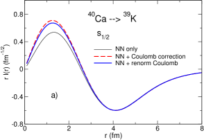
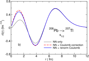
Figure 1: The overlap functions $rI_{lj}(r)$ for $s_{1/2}$ proton removal from ⁴⁰Ca ($a$) and ²⁰⁸Pb ($b$) targets calculated in the STA with nuclear NN interaction only (thin line) and with adding the original (dashed line) and renormalised (solid line) Coulomb corrections.

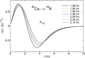
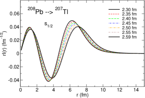
Figure 2: The overlap functions $rI_{lj}(r)$ for $s_{1/2}$ proton removal from ⁴⁰Ca ($a$) and ²⁰⁸Pb ($b$) targets calculated in the STA with NN interaction only for several values of the oscillator radius.

Another important input to the STA is the oscillator radius $b$ used to generate harmonic oscillator single-particle wave functions. In previous studies of light $0p$-shell nuclei [9, 10, 12] this radius has been taken from electron elastic scattering. Investigation of sensitivity of the overlap functions to the choice of $b$, carried out for ¹⁶O in [10], has shown that SFs and ANC can change within a factor of two when $1.5<b<2$ fm. No investigation of $b$-dependence was carried out for $A\geq 16$ nuclei in [11]. The oscillator radius $b$ used there was fixed by the $\hbar\omega=41A^{-1/3}-25A^{-2/3}$ relation proposed in [20] which claims that it reasonably reproduces nuclear charge radii. However, analysis of proton scattering on a wide range of nuclei [25, 24, 23, 22, 21] suggests that $b$ can be significantly smaller. For example, the $\hbar\omega=41A^{-1/3}-25A^{-2/3}$ formula gives 2.06 and 2.15 fm for ⁴⁰Ca and ⁴⁸Ca, respectively, while [21] suggests $b=1.9$ fm for both isotopes. A smaller value of $b=1.869$ fm was used in [25] for ⁴⁸Ca and a larger value of $b=2.0$ fm was used in [23] for ⁴⁰Ca. For ²⁰⁸Pb, the $\hbar\omega=41A^{-1/3}-25A^{-2/3}$ prescription gives $b=2.59$ fm while [25] and [24] recommend 2.326 fm and $b=A^{1/6}=2.434$ fm, respectively. Fig. 2 compares overlap functions for $s_{1/2}$ proton removal from ⁴⁰Ca and ²⁰⁸Pb, calculated using NN force only, as a function of oscillator radius. Since both these overlap functions have nodes they are sensitive to the choice of $b$. This can affect the spectroscopic factors and, most significantly, the ANCs, which is demonstrated in Fig. 3. While spectroscopic factors change within 30$\%$ and 24$\%$ for ⁴⁰Ca and ²⁰⁸Pb, respectively, the corresponding change in squared ANCs is within 87$\%$ and a factor of 4, which could be completely devastating for peripheral processes. The sensitivity of the r.m.s. radius of both overlap functions is much smaller.

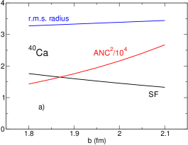
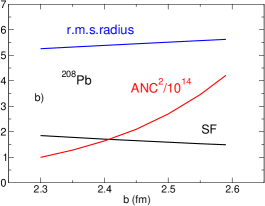
Figure 3: The spectroscopic factor (SF), ANC squared (in fm^-1) and r.m.s. radius (in fm) for $s_{1/2}$ proton removal from ⁴⁰Ca ($a$) and ²⁰⁸Pb ($b$) targets as a function of the oscillator radius $b$, calculated in the STA with NN interaction only.

5 Numerical calculations with 3N force

First of all, the dependence of the source term, and the corresponding contribution to the overlap function, on the choice of the range $\rho_{0}$ of the 3N force was investigated. Figure 4 shows this dependence for the case of the $s_{1/2}$ proton removal from ⁴⁰Ca and ²⁰⁸Pb, demonstrated for the contribution from the $W^{(0)}_{123}$ term only. The overlap functions calculated with different $\rho_{0}$ were normalized to have the same value in the first maximum. For both nuclei increasing $\rho_{0}$ leads to a larger second maximum and moves the position of the first node towards smaller $r$. For ²⁰⁸Pb, the third maximum first decreases at $0<\rho_{0}<0.5$ fm but then increases for $\rho_{0}>0.5$ fm. For both nuclei the nodes of $I_{lj}(r)$ are closer to the origin than those of the overlaps generated by the NN force only. This means that if the NN force does not reproduce the magnitude of the asymptotic part of $I_{lj}(r)$, corresponding to experimentally determined ANCs, the empirical 3N force needed to correct this magnitude would have a large range $\rho_{0}$.

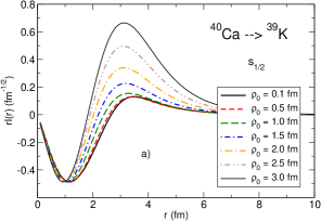
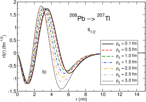
Figure 4: The contribution to the overlap function $rI_{lj}(r)$ corresponding to the 3N force $W^{(0)}_{123}$ calculated for $s_{1/2}$ proton removal from ⁴⁰Ca ($a$) and ²⁰⁸Pb ($b$) targets for several ranges $\rho_{0}$ of the 3N force. The depths $W_{0}$ are chosen to give the same value for the overlap function in the first maximum for each $\rho_{0}$.

Next, the relative contributions from different components of the 3N force have been studied. Figure 5 shows these contributions calculated for $s_{1/2}$ proton removal from ⁴⁰Ca and ²⁰⁸Pb using $\rho_{0}=2$ fm and the depth of 1 MeV for all four components of the 3N force. For ⁴⁰Ca the contributions from $W^{(\sigma)}$ and $W^{(\tau)}$ are the same, being exactly one-third of the contribution from $W^{(\sigma\tau)}$. The same has been observed for removals of nucleons with other $l$ and $j$ involving ¹⁶O and ⁴⁰Ca. These nuclei have a well defined value of the spin $S=0$ (associated with the operator $\vec{S}=\sum\limits_{i}\vec{s}_{i}$ and not to be confused with the total angular momentum $J$) and isospin $T=0$. For other double-closed shell nuclei considered here, where $S$ is not a good quantum number, such relations between the corresponding components do not hold any longer. For example, for ²⁰⁸Pb the proportions between the values of the first, second and third maximum are different for all four components of the 3N force, which could be helpful when fitting it to get the correct positions of the nodes of the overlap. In all cases considered the contribution from $W^{(0)}$ has a different sign to those coming from $W^{(\sigma)}$, $W^{(\tau)}$ and $W^{(\sigma\tau)}$ and is not proportional to them.

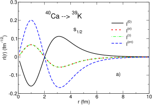
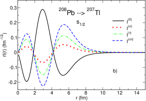
Figure 5: The contribution to the overlap function corresponding to the 3N force components $W^{(0)}$, $W^{(\sigma)}$, $W^{(\tau})$ and $W^{(\sigma\tau)}$, calculated for $s_{1/2}$ proton removal from the ⁴⁰Ca ($a$) and ²⁰⁸Pb ($b$) targets using $\rho_{0}$ = 2 fm. The oscillator radii employed are $b=$1.90 fm and 2.38 fm for ⁴⁰Ca and ²⁰⁸Pb, respectively.

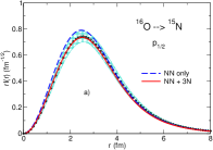
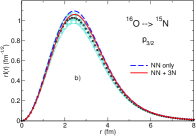
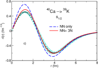
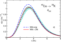
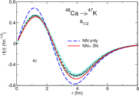
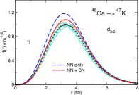
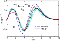
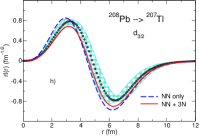
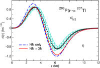
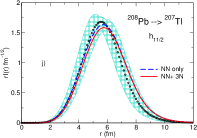
Figure 6: One-proton removal overlap functions for ⁴⁰Ca ($a,b)$, ⁴⁸Ca ($c,d$) and ²⁰⁸Pb $(e,f,g,h)$, calculated with NN force only and with including the 3N force having $W_{0}=1$ MeV and $\rho_{0}=2$ fm.

As a next step it was investigated how strong the 3N force should be to give reasonable predictions for the overlap functions for proton knockout from double-magic nuclei ¹⁶O, ^40,48Ca and ²⁰⁸Pb. Phenomenological overlaps determined from the $(e,e^{\prime}p)$ reactions on these targets are available in [26] where they are represented by the single-particle wave functions, satisfying two-body Schrödinger equation with experimental separation energies, times the spectroscopic amplitudes. Such a representation guarantees that the overlaps have a correct asymptotic decrease. The radius $r_{0}$ and diffuseness $a$ of the potential well used to calculate the single-particle wave functions are given in Tables 1 and 3 of [26], together with the spectroscopic factors $S_{lj}$. Both $r_{0}$ and $S_{lj}$ are given together with their uncertainty ranges. The corresponding overlaps also have uncertainties that can be large, as seen in figures 6a to 6h. In these figures the overlaps corresponding to the mean values of the parameters $r_{0}$ and $S_{lj}$ are shown by open circles while all other possible values are collected in a band.

In most cases shown in Fig. 6 the overlaps calculated with NN force only are outside the phenomenologically determined bands, which is partially due to the choice of the oscillator radius. The calculations with NN force used smaller oscillator radii than those employed in all previous STA publications and they were based on the proton scattering work of [25, 24, 23, 22, 21] being 1.8 fm for ¹⁶O, 1.90 fm for ^40,48Ca and 2.38 fm ²⁰⁸Pb. Larger oscillator radii lead to larger overlaps outside the nuclear interior so that unrealistically large ranges of the 3N force are needed to bring them down. It was found out that adding only one component of the 3N force, $W^{(0)}$, with a depth $W_{0}=1$ MeV and a range $\rho_{0}=2$ fm is sufficient to get an improved description of the phenomenological overlaps for all considered final states populated by proton knockout from ¹⁶O, ^40,48Ca and ²⁰⁸Pb, which is shown in Fig. 6. An alternative single-term 3N potential with $W^{\sigma\tau}_{0}=-0.9$ MeV and $\rho_{0}=2$ fm gives a similar quality (or slightly better) description of the phenomenological overlaps for ^40,48Ca and ²⁰⁸Pb but a worse description for ¹⁶O. It should be noticed that for any individual overlap function it is possible to tune the 3N force to locate $I_{lj}(r)$ within the limits of the phenomenological band. However, there is no point is making such an effort at present since the method itself would lose predictability. More important is to understand if a universal effective 3N force exists that would be applicable to all nuclei. However, this is a task for the future.

Table 1: The STA spectroscopic factors for the overlap functions $\langle A|A-1\rangle$ obtained with NN force only ($S_{lj}^{NN}$) and with including 3N force ( $S_{lj}^{(NN+3N)}$). The spectroscopic factors obtained from analysis of $(e,e^{\prime}p)$ reaction for ¹⁶O, ^40,48Ca and ²⁰⁸Pb are shown in the last column. Also shown are the quantum numbers $lj$ of the removed nucleon, the excitation energy $E_{x}$ of $A-1$, the separation energy $\varepsilon$ of the removed nucleon (both in MeV) and the spectroscopic factor $S^{\rm SM}_{lj}$ of the $0\hbar\omega$ shell model. For ^16,24O, ^40,48Ca, ⁵⁶Ni and proton removal from ¹³²Sn the shell model spectroscopic factors include correction for centre-of-mass motion.

$A$	$A$$-$1	$lj$	$E_{x}$	$\varepsilon$	$S^{\rm SM}_{lj}$	$S_{lj}^{(NN)}$	$S_{lj}^{(NN+3N)}$	$S_{lj}^{(e,e^{\prime}p)}$
16O	15N	$p_{1/2}$	0.0	12.13	2.133	1.42	1.23	1.27(13)
		$p_{3/2}$	6.32	18.45	4.267	2.56	2.40	2.25(22)
16O	15O	$p_{1/2}$	0.0	15.66	2.133	1.38	1.17
		$p_{3/2}$	6.18	21.84	4.267	2.53	2.35
24O	23N	$p_{1/2}$	0.0	26.6	2.087	1.29	1.04
24O	23O	$s_{1/2}$	0.0	3.6	2.177	1.67	1.28
40Ca	39K	$d_{3/2}$	0.0	8.33	4.208	3.12	2.63	2.58(19)
		$s_{1/2}$	2.52	10.85	2.104	1.53	1.12	1.03(7)
40Ca	39Ca	$d_{3/2}$	0.0	15.64	4.208	3.06	2.54
		$s_{1/2}$	2.47	18.11	2.104	1.58	1.05
48Ca	47K	$s_{1/2}$	0.0	15.81	2.086	1.68	1.18	1.07(7)
		$d_{3/2}$	0.36	16.17	4.172	3.18	2.64	2.26(16)
48Ca	47Ca	$f_{7/2}$	0.0	9.95	8.523	5.24	4.79
56Ni	55Co	$f_{7/2}$	0.0	7.17	8.444	5.44	5.00
56Ni	55Ni	$f_{7/2}$	0.0	16.64	8.444	5.31	4.83
132Sn	131In	$g_{9/2}$	0.0	15.71	8.247	6.76	6.16
132Sn	131Sn	$d_{3/2}$	0.0	7.31	4.0	3.73	2.52
208Pb	207Tl	$s_{1/2}$	0.0	8.00	2.0	1.64	1.04	0.98(9)
		$d_{3/2}$	0.35	8.35	4.0	3.28	2.52	2.31(22)
		$h_{11/2}$	1.35	9.35	12.	7.24	6.70	6.85(68)
		$d_{5/2}$	1.67	9.67	6.0	5.00	4.22	2.93(28)
		$g_{7/2}$	3.47	11.47	8.0	6.36	5.55	2.06(20)
208Pb	207Pb	$p_{1/2}$	0.0	7.37	2.0	1.79	0.83

The spectroscopic factors corresponding to the overlaps with NN force only and with added spin- and isospin-independent 3N contribution $W^{(0)}$ are shown in Table 1. For proton removal from ¹⁶O, ^40,48Ca and ²⁰⁸Pb, the spectroscopic factors either agree or are very close to those extracted from the $(e,e^{\prime}p)$ study, except for removing $g_{7/2}$ proton from ²⁰⁸Pb. They are reduced with respect to the $0\hbar\omega$ shell model values (see Table 1), which for double-magic nuclei are the same as those given by the independent particle model. To investigate if there is any asymmetry in the spectroscopic factor reductions the overlap functions for neutron removal were also calculated for the same targets. Three more cases involving unstable nuclei, ²⁴O, ⁵⁶Ni and ¹³²Sn, where the difference between the proton and neutron separation energies is larger, were added to this study. The oscillator radii for these nuclei were chosen to be 1.85, 1.92 and 2.15 fm, respectively. The ratio of the STA spectroscopic factors to those obtained in the $0\hbar\omega$ shell model is shown in Fig. 7 as a function of the difference between the proton and neutron (or neutron and proton for neutron removal) separation energies $\Delta S$. For ¹⁶O, ⁴⁰Ca and ⁵⁶Ni there is practically no asymmetry both with and without the 3N force. Strong and unusual asymmetry predicted for ⁴⁸Ca with NN force only disappears when the 3N force is added. For the case of ²⁴O, with the largest $\Delta S$, the asymmetry seen in $S_{\rm STA}/S_{\rm SM}$ calculated with NN force only also becomes smaller when 3N force is added. The case of ¹³²Sn is very unusual. Without 3N force, the reduction factor $S_{\rm STA}/S_{\rm SM}$ is 0.93 and 0.83 for neutron and a more strongly bound proton, respectively. However, the contribution from the 3N force is larger for neutron than for proton removal so that adding 3N force makes neutron spectroscopic strength reduction stronger than the one for proton. This conflicts with experimental observations made with knockout reactions in [15] suggesting that a different choice of 3N should take place. Indeed, with the second single-term 3N force choice mentioned above, $W^{(\sigma\tau)}_{0}=-0.9$ MeV and $\rho_{0}=2$ fm, the $S_{\rm STA}/S_{\rm SM}$ ratio becomes very similar for neutron and proton, being 0.73 and 0.76, respectively, suggesting no asymmetry in the spectroscopic strength reduction. Not shown in Fig. 7 is the ²⁰⁸Pb case where, as in the case of ¹³²Sn, the 3N contribution is much stronger than that in the proton case leading to the $S_{\rm STA}/S_{\rm SM}$ value of 0.41 which at first sight seems to be unrealistic. With the second choice of the 3N force, $W^{(\sigma\tau)}_{0}=-0.9$ MeV and $\rho_{0}=2$ fm, the spectroscopic factor is 1.08 and 1.09 for neutron and proton, respectively, with the same ratio $S_{\rm STA}/S_{\rm SM}=0.54$ for both.

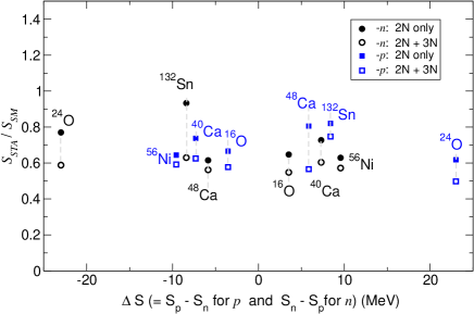
Figure 7: The ratio $S_{\rm STA}/S_{\rm SM}$ for neutron and proton removals from ^16,24O, ^40,48Ca, ⁵⁶Ni and ¹³²Sn, calculated with NN force only and with including the 3N force having $W_{0}=1$ MeV and $\rho_{0}=2$ fm. The ratios are shown as functions of difference $\Delta S$ between the proton ($S_{p}$) and neutron ($S_{n}$) separation energies.

The ANCs and r.m.s. radii for the overlaps from Table 1 are shown in Table 2. One can see that including the 3N force gives smaller values of the ANC $C_{lj}$ and larger radii. The single-particle ANCs $b_{lj}=C_{lj}/\sqrt{S_{lj}}$ can be either smaller of larger than those obtained without 3N force. The coefficients $b_{lj}$ give an idea about the width of the effective potential well that would be needed to generate the overlaps in a two-body model. Including 3N force does not have a unique effect on this width. There is not much information on experimental ANCs for the nuclei considered here, apart from the proton removal from ¹⁶O. The $(^{3}He,d)$ reaction study in [27] gives $C^{2}_{lj}=298(63)$ fm^-1 for the ground state of ¹⁵N while a corrected value of this ANC from Ref. [28], based on the updated value of the ANC for ³He, is $C^{2}_{lj}=175(29)$ fm^-1. The latter covers both the NN and NN+3N values of the ANC obtained in the STA. Also, the r.m.s. radius for the $\langle^{15}$N$|^{16}$O$\rangle$ overlap, calculated with NN+3N force, agrees with the experimental values 2.943(30) and 2.719(24) fm for $\frac{1}{2}^{-}$ and $\frac{3}{2}^{-}$ states, respectively, obtained in [29].

Table 2: The ANC $C_{lj}$, single-particle ANC $b_{lj}$ (both in fm^-1/2) and the r.m.s. radius (in fm) of the overlap functions $\langle A|A-1\rangle$ obtained in STA with NN force only and with including 3N force. The quantum numbers $lj$ of the removed nucleon are shown in the third column and eN denotes 10^N.

			NN			NN + 3N
$A$	$A$$-$1	$lj$	$C_{lj}$	$b_{lj}$	$\langle r^{2}\rangle^{1/2}$	$C_{lj}$	$b_{lj}$	$\langle r^{2}\rangle^{1/2}$
16O	15N	$p_{1/2}$	13.4	11.2	2.871	12.9	11.6	2.905
		$p_{3/2}$	35.6	22.2	2.774	33.1	21.4	2.791
16O	15O	$p_{1/2}$	10.7	9.11	2.823	10.2	9.43	2.866
		$p_{3/2}$	26.8	16.8	2.744	26.3	17.2	2.767
24O	23N	$p_{1/2}$	70.4	62.0	2.830	67.8	66.5	2.903
24O	23O	$s_{1/2}$	-3.51	-2.72	3.400	-3.15	-2.78	3.445
40Ca	39K	$d_{3/2}$	57.8	32.7	3.554	55.6	34.3	3.616
		$s_{1/2}$	-132.	-107.	3.392	-123.	-116.	3.527
40Ca	39Ca	$d_{3/2}$	22.8	13.0	3.482	21.9	13.7	3.551
		$s_{1/2}$	-48.6	-38.7	3.131	-45.1	-44.0	3.380
48Ca	47K	$s_{1/2}$	-258.	-199.	3.501	-242.	-222.	3.695
		$d_{3/2}$	162.	90.7	3.493	157.	96.4	3.567
48Ca	47Ca	$f_{7/2}$	7.69	3.36	3.934	7.53	3.44	3.966
56Ni	55Co	$f_{7/2}$	146.	62.7	3.978	144.	64.3	4.008
56Ni	55Ni	$f_{7/2}$	31.8	13.8	3.909	31.3	14.2	3.948
132Sn	131In	$g_{9/2}$	1.32e4	5.08e3	4.875	1.30e4	5.24e3	4.927
132Sn	131Sn	$d_{3/2}$	-24.5	-12.3	4.867	-22.3	-13.5	5.218
208Pb	207Tl	$s_{1/2}$	1.21e7	9.45e6	5.488	1.15e7	1.13e7	5.943
		$d_{3/2}$	-9.33e6	-5.15e6	5.507	-9.21e6	-5.80e6	5.785
		$h_{11/2}$	1.93e6	7.17e5	5.867	1.92e6	7.42e5	5.919
		$d_{5/2}$	-8.24e6	-3.69e6	5.481	-8.11e6	-3.95e6	5.674
		$g_{7/2}$	2.14e6	8.49e5	5.486	2.12e6	9.00e5	5.579
208Pb	207Pb	$p_{1/2}$	47.6	35.6	5.176	41.6	45.7	6.094

6 Summary and future perspectives

In this work, an effective 3N force has been introduced into the source term approach designed to generate one-nucleon overlap functions for various nucleon-removal reactions. This force acts between the removed nucleon and two nucleons of the residual nucleus and it arises because the STA uses nuclear wave functions calculated in a truncated model space, more specifically, the one given by the 0$\hbar\omega$ shell model. The 3N force in STA is not equal to the 3N force that could be employed in modelling many-body nuclear wave functions in exactly the same way as the 2N force between the removed nucleon and one nucleon in the residual nucleus in STA is not the same as the effective 2N force employed in the wave function calculations [9, 10]. Although, in principle, an STA-rated induced 3N force could be calculated in a microscopic approach such a task would require a major effort. Therefore, this paper adopts a phenomenological approach in choosing such a force assuming that it has four components determined by a different spin and isospin content and has a form given by a hypercentral gaussian potential.

The first application of the effective 3N force have been made here for one-proton removal from double-magic nuclei ¹⁶O, ^40,48Ca and ²⁰⁸Pb where phenomenological overlap functions are available from the $(e,e^{\prime}p)$ study. The calculations revealed that only one component, spin- and isospin-independent, with the hypercentral range of 2 fm and a depth of 1 MeV is sufficient to improve description of these phenomenological overlaps. The corresponding spectroscopic factors either agree with or are very close to the $(e,e^{\prime}p)$ values. These spectroscopic factors are reduced with respect to those given by the independent particle model, or the $0\hbar\omega$ shell model. Reduction is also predicted for one-neutron removal from the same double-magic nuclei and for ¹⁶O and ⁴⁰Ca it is in the same proportions both for neutrons and protons irrespective of the presence of the 3N force, which slightly decreases these spectroscopic factors. However, for ⁴⁸Ca a large asymmetry in reduction is seen with the 2N force only, which is removed when 3N force is included. Including spin- and isospin-independent 3N force leads to unusual $S_{\rm STA}/S_{\rm SM}$ results for heavier nuclei ¹³²Sn and ²⁰⁸Pb. A different choice of the 3N force, represented by a forth term in Eq. (11), suggests no asymmetry in spectroscopic factor reduction in these nuclei.

Whether the spectroscopic factor reduction in STA can be reliably studied for an arbitrary nucleus depends on the existence of a universal effective 3N force applicable to a wide range of atomic nuclei. No attempts to find such a force have been made here because of several reasons. 1) Better quality data on “experimental” overlap functions are needed. Currently, available phenomenological overlaps have large experimental and systematic uncertainties. However, reducing these uncertainties is a challenging task because the overlap functions are not observables and they can only be indirectly deduced from reaction data analysis. 2) The STA overlaps depend, in the first instance, on the effective 2N force and harmonic oscillator radius. Any attempts of fitting the 3N force should be accompanied by fitting 2N force as well. At the moment, in all previous publications the 2N force was fixed. However, it could be possible to find a better representation of this force, in particular, it could depend on oscillator radius as well so that the resulting overlaps would not be subjected to strong variations with this radius. 3) The hypercentral gaussian functional form used in this work for effective 3N force may not represent it in the most optimal way. Other options, such as a symmetrized product of two NN formfactors should also be explored together with other structures such as those mimicking double-pion exchange. Future work will tackle these issues.

Finally, going beyond the $0\hbar\omega$ approximation for nuclear models on $A$ and $A-1$ can be very important for the further development of the STA. It will allow the wave functions to be used which describe better the internal nuclear region, in particular, it can also reduce the dependence of the STA overlaps on the oscillator radius choices. While it could be difficult to do it for medium-mass nuclei, for light nuclei this is certainly possible. Having a good STA-rated 2N and 3N effective interactions consistent with extended model space will make it possible to predict the overlap functions between any nuclear states accessible to extended shell model studies.

Appendix A STA matrix elements of the 3N interaction.

A.1 Spatial part

We will first derive an expression to evaluate the spacial part

$$\langle\varphi_{n^{\prime}_{1}l^{\prime}_{1}m^{\prime}_{1}}(\mbox{\boldmath$r$}_{1})\varphi_{n^{\prime}_{2}l^{\prime}_{2}m^{\prime}_{2}}(\mbox{\boldmath$r$}_{2})e^{i\mbox{\boldmath$k$}\mbox{\boldmath$r$}_{3}}\mid W_{123}\mid\varphi_{n_{1}l_{1}m_{1}}(\mbox{\boldmath$r$}_{1})\varphi_{n_{2}l_{2}m_{2}}(\mbox{\boldmath$r$}_{2})\varphi_{n_{3}l_{3}m_{3}}(\mbox{\boldmath$r$}_{3})\rangle$$ (14)

of the matrix element (10) assuming that the 3N force $W_{123}$ has a hypercentral form given by Eq. (12). The matrix element (10) is evaluated in the harmonic oscillator basis defined by the single-particle wave functions $\varphi_{nlm}(\mbox{\boldmath$r$})=\varphi_{nl}(r)Y_{lm}(\hat{\mbox{\boldmath$r$}})$ with the radial part

$$\varphi_{nl}(r)=\frac{1}{b^{3/2}}\sqrt{\frac{2n!}{\Gamma\left(n+l+\frac{3}{2}\right)}}\left(\frac{r}{b}\right)^{l}e^{-\frac{r^{2}}{2b^{2}}}L_{n}^{l+1/2}\left(\frac{r^{2}}{b^{2}}\right),$$ (15)

where $b$ is the oscillator length. We will also need harmonic oscillator wave functions

$$\phi_{nlm}(\mbox{\boldmath$q$})=(-)^{n}i^{l}(2\pi)^{3/2}\phi_{nl}(q)Y_{lm}(\hat{\mbox{\boldmath$q$}})$$ (16)

in momentum space with $\phi_{nl}(q)$ given by Eq. (15) in which the substitution $b\rightarrow 1/b$ is made. As a first step to evaluate (14) we apply relation

$$\varphi^{*}_{n^{\prime}l^{\prime}m^{\prime}}(\mbox{\boldmath$r$})\varphi_{nlm}(\mbox{\boldmath$r$})=\sum_{\nu NLM}(-)^{m^{\prime}}(l^{\prime}-m^{\prime}lm|LM)\langle\nu 0NL:L|n^{\prime}l^{\prime}nl:L\rangle$$

$$\,\,\,\,\,\,\,\,\,\,\,\,\,\,\,\,\,\,\,\,\,\,\,\,\,\,\,\,\,\,\,\,\,\,\,\,\,\,\,\,\,\,\,\,\,\,\,\times\varphi_{\nu 00}(0)\varphi_{NLM}(\sqrt{2}\mbox{\boldmath$r$})$$ (17)

to the products of wave functions of the same coordinates, which are either $\mbox{\boldmath$r$}_{1}$ or $\mbox{\boldmath$r$}_{2}$. In Eq. (17) the $\langle\nu 0NL:L|n^{\prime}l^{\prime}nl:L\rangle$ is the Moshinsky bracket for particle with equal masses [30]. Introducing new variables, the normalized Jacobi coordinates $\mbox{\boldmath$\xi$}_{1}=(\mbox{\boldmath$r$}_{1}-\mbox{\boldmath$r$}_{2})/\sqrt{2}$ and $\mbox{\boldmath$\xi$}_{2}=\sqrt{\frac{2}{3}}\left(\frac{1}{\sqrt{2}}\mbox{\boldmath$X$}_{12}-\mbox{\boldmath$r$}_{3}\right)$, and applying the Moshinsky transformation again to the function of $\mbox{\boldmath$r$}_{1}$ and $\mbox{\boldmath$r$}_{2}$we get

$$\langle\varphi_{n^{\prime}_{1}l^{\prime}_{1}m^{\prime}_{1}}(\mbox{\boldmath$r$}_{1})\varphi_{n^{\prime}_{2}l^{\prime}_{2}m^{\prime}_{2}}(\mbox{\boldmath$r$}_{2})e^{i\mbox{\boldmath$k$}\mbox{\boldmath$r$}_{3}}\mid W_{123}\mid\varphi_{n_{1}l_{1}m_{1}}(\mbox{\boldmath$r$}_{1})\varphi_{n_{2}l_{2}m_{2}}(\mbox{\boldmath$r$}_{2})\varphi_{n_{3}l_{3}m_{3}}(\mbox{\boldmath$r$}_{3})\rangle$$

$$=\sum\,\,(-)^{m^{\prime}_{1}}(l^{\prime}_{1}-m^{\prime}_{1}l_{1}m_{1}|L_{1}M_{1})\,\langle\nu_{1}0N_{1}L_{1}:L_{1}|n^{\prime}_{1}l^{\prime}_{1}n_{1}l_{1}:L_{1}\rangle\,\varphi_{\nu_{1}00}(0)$$

$$\,\,\,\,\,\,\,\,\,\,\,\,\,\,\,\,\,\times(-)^{m^{\prime}_{2}}(l^{\prime}_{2}-m^{\prime}_{2}l_{2}m_{2}|L_{2}M_{2})\,\langle\nu_{2}0N_{2}L_{2}:L_{2}|n^{\prime}_{2}l^{\prime}_{2}n_{2}l_{2}:L_{2}\rangle\,\varphi_{\nu_{2}00}(0)$$

$$\,\,\,\,\,\,\,\,\,\,\,\,\,\,\,\,\,\times(L_{1}M_{1}L_{2}M_{2}|L_{12}M_{12})(\lambda\mu\,L_{3}M_{3}|L_{12}M_{12})\langle\nu\lambda N^{\prime}_{3}L_{3}:L_{12}|N_{1}L_{1}N_{2}L_{2}:L_{12}\rangle$$

$$\times{W}_{0}\int d\mbox{\boldmath$\xi$}_{1}d\mbox{\boldmath$X$}_{12}d\mbox{\boldmath$r$}_{3}\,e^{-i\mbox{\boldmath$k$}\mbox{\boldmath$r$}_{3}}e^{-\frac{\xi_{1}^{2}+\xi_{2}^{2}}{\rho_{0}^{2}}}\varphi_{\nu\lambda\mu}(\sqrt{2}\mbox{\boldmath$\xi$}_{1})\varphi_{N^{\prime}_{3}L_{3}M_{3}}(\sqrt{2}\mbox{\boldmath$X$}_{12})\varphi_{n_{3}l_{3}m_{3}}(\mbox{\boldmath$r$}_{3}),$$ (18)

where the sum runs over $\{\nu_{1}N_{1}L_{1}\nu_{2}N_{2}L_{2}\nu\lambda{\tilde{n}}^{\prime}_{3}l^{\prime}_{3}\}$ and $\{M_{1}M_{2}M_{3}\mu m^{\prime}_{3}\}$. We proceed with integrating over $d\mbox{\boldmath$\xi$}_{1}$ using

$$\int d\mbox{\boldmath$\xi$}_{1}e^{-\frac{\xi_{1}^{2}}{\rho_{0}^{2}}}\varphi_{\nu\lambda\mu}(\sqrt{2}\mbox{\boldmath$\xi$}_{1})=w_{\nu}\delta_{\lambda,0}\delta_{\mu,0}.$$ (19)

Then we aim to make an integration over $d\mbox{\boldmath$X$}_{12}$. For this purpose we note that $e^{-\xi^{2}_{2}/\rho_{0}^{2}}=\sqrt{2\pi\Gamma(\frac{3}{2})}\varphi_{000}\left(\frac{\sqrt{2}b}{\rho_{0}}\mbox{\boldmath$\xi$}_{2}\right)$. Introducing another variable change, $\mbox{\boldmath$y$}_{1}=\alpha\sqrt{2}\mbox{\boldmath$X$}_{12}-\beta\frac{\sqrt{2}b}{\rho_{0}}\mbox{\boldmath$\xi$}_{2}$ and $\mbox{\boldmath$y$}_{2}=\beta\sqrt{2}\mbox{\boldmath$X$}_{12}+\alpha\frac{\sqrt{2}b}{\rho_{0}}\mbox{\boldmath$\xi$}_{2}$ with $\alpha=(1+\frac{3\rho_{0}^{2}}{b^{2}})^{-1/2}$ and $\beta=(1+\frac{b^{2}}{3\rho_{0}^{2}})^{-1/2}$, we rearrange the product $e^{-\xi^{2}_{2}/\rho_{0}^{2}}\varphi_{N^{\prime}_{3}L_{3}M_{3}}(\sqrt{2}\mbox{\boldmath$X$}_{12})$ using Moshinsky technique for particle with different masses [31]

$$|\varphi_{N^{\prime}_{3}L_{3}}(\sqrt{2}\mbox{\boldmath$X$}_{12})\varphi_{00}\left(\frac{\sqrt{2}b}{\rho_{0}}\mbox{\boldmath$\xi$}_{2}\right):L_{3}M_{3}\rangle$$

$$=\sum_{N_{3}N}\langle N_{3}L_{3}NL:L_{3}|d_{1}|N^{\prime}_{3}L_{3}00:L_{3}\rangle|\varphi_{N_{3}L_{3}}(2\alpha\mbox{\boldmath$r$}_{3})\varphi_{NL}(\mbox{\boldmath$y$}_{2}):L_{3}M_{3}\rangle,$$ (20)

where $d_{1}=\frac{b^{2}}{3\rho_{0}^{2}}$. The numerical values of the Moshinsky brackets $\langle N_{3}L_{3}NL:L_{3}|d_{1}|00N^{\prime}_{3}L_{3}:L_{3}\rangle$ were calculated using the formalism and the Fortran code from [32]. After integration over $d\mbox{\boldmath$X$}_{12}$ we integrate over $d\mbox{\boldmath$r$}_{3}$ and obtain

$$\int d\mbox{\boldmath$r$}_{3}\,\varphi_{N_{3}L_{3}M_{3}}(2\alpha\mbox{\boldmath$r$}_{3})e^{-i\mbox{\boldmath$k$}\mbox{\boldmath$r$}_{3}}\varphi_{n_{3}l_{3}m_{3}}(\mbox{\boldmath$r$}_{3})=(-)^{l^{\prime}_{3}}\,\theta^{3}\sum_{\nu_{3}N_{3}L_{3}M_{3}n^{\prime}_{3}l^{\prime}_{3}m^{\prime}_{3}}(L_{3}M_{3}l_{3}m_{3}|l^{\prime}_{3}m^{\prime}_{3})$$

$$\times\langle\nu_{3}0n^{\prime}_{3}l^{\prime}_{3}:l^{\prime}_{3}|d_{2}|N_{3}L_{3}n_{3}l_{3}:l^{\prime}_{3}\rangle\varphi_{\nu_{3}00}(0)\phi_{n^{\prime}_{3}l^{\prime}_{3}m^{\prime}_{3}}\left(\theta\mbox{\boldmath$k$}\right),$$ (21)

where $d_{2}=(4\alpha^{2})^{-1}$, $\theta=(1+4\alpha^{2})^{-1/2}$. This leads to the final result for the matrix element (18),

$$\langle\varphi_{n^{\prime}_{1}l^{\prime}_{1}m^{\prime}_{1}}(\mbox{\boldmath$r$}_{1})\varphi_{n^{\prime}_{2}l^{\prime}_{2}m^{\prime}_{2}}(\mbox{\boldmath$r$}_{2})e^{i\mbox{\boldmath$k$}\mbox{\boldmath$r$}_{3}}\mid W_{123}\mid\varphi_{n_{1}l_{1}m_{1}}(\mbox{\boldmath$r$}_{1})\varphi_{n_{2}l_{2}m_{2}}(\mbox{\boldmath$r$}_{2})\varphi_{n_{3}l_{3}m_{3}}(\mbox{\boldmath$r$}_{3})\rangle$$

$$=\sum\,\,(-)^{m^{\prime}_{1}+m^{\prime}_{2}+m^{\prime}_{3}}(l^{\prime}_{1}-m^{\prime}_{1}l_{1}m_{1}|L_{1}M_{1})\,(l^{\prime}_{2}-m^{\prime}_{2}l_{2}m_{2}|L_{2}M_{2})\,(l^{\prime}_{3}-m^{\prime}_{3}l_{3}m_{3}|L_{3}M_{3})\,$$

$$\,\,\,\,\,\,\,\,\,\,\,\,\,\,\,\,\,\times(-)^{L_{3}+M_{3}}\hat{L}_{3}^{-1}(L_{1}M_{1}L_{2}M_{2}|L_{3}-M_{3})\,W_{\gamma_{1}\gamma_{2}\gamma_{3}}\,\phi_{n^{\prime}_{3}l^{\prime}_{3}m^{\prime}_{3}}\left(\theta\mbox{\boldmath$k$}\right),$$ (22)

where $\gamma_{i}=\{n^{\prime}_{i}l^{\prime}_{i}n_{i}l_{i}L_{i}\}$, $i=1,2,3$ and

$$W_{\gamma_{1}\gamma_{2}\gamma_{3}}=\left(\frac{\sqrt{\pi}}{2}\,b\beta^{2}\theta^{2}\right)^{\frac{3}{2}}\,\hat{l}^{\prime}_{3}{W}_{0}\sum_{N_{1}N_{2}N_{3}N^{\prime}_{3}N\nu_{1}\nu_{2}\nu_{3}\nu}w_{\nu}\phi_{N00}(0)\varphi_{\nu_{1}00}(0)\varphi_{\nu_{2}00}(0)\varphi_{\nu_{3}00}(0)$$

$$\times\langle\nu_{1}0N_{1}L_{1}{\rm:}L_{1}|n^{\prime}_{1}l^{\prime}_{1}n_{1}l_{1}{\rm:}L_{1}\rangle\,\langle\nu_{2}0N_{2}L_{2}{\rm:}L_{2}|n^{\prime}_{2}l^{\prime}_{2}n_{2}l_{2}{\rm:}L_{2}\rangle\,\langle\nu 0N^{\prime}_{3}L_{3}{\rm:}L_{3}|N_{1}L_{1}N_{2}L_{2}{\rm:}L_{3}\rangle\,$$

$$\times\langle N_{3}L_{3}N0{\rm:}L_{3}|d_{1}|N^{\prime}_{3}L_{3}00{\rm:}L_{3}\rangle\langle\nu_{3}0n^{\prime}_{3}l^{\prime}_{3}{\rm:}l^{\prime}_{3}|d_{2}|N_{3}L_{3}n_{3}l_{3}{\rm:}l^{\prime}_{3}\rangle.$$ (23)

The summation in (22) is performed over $\{n^{\prime}_{3}l^{\prime}_{3}m^{\prime}_{3}L_{1}L_{2}L_{3}\}$ while $M_{i}=m_{i}-m^{\prime}_{i}$ for all $i=1,2,3$. It should be noted that (22) is in fact an expansion over a finite number of single-particle harmonic oscillator wave functions $\phi_{n^{\prime}_{3}l^{\prime}_{3}m^{\prime}_{3}}$ of an argument $\theta\mbox{\boldmath$k$}$ that depends on the range of the 3N interaction. In Eq. (22) $2n^{\prime}_{3}+l^{\prime}_{3}$ changes from 0 to $2n_{1}+l_{1}+2n_{2}+l_{2}+2n_{3}+l_{3}+2n^{\prime}_{1}+l^{\prime}_{1}+2n^{\prime}_{2}+l^{\prime}_{2}$. In principle, the matrix element (18) could be sought for as an expansion over the basis $\phi_{n^{\prime}_{3}l^{\prime}_{3}m^{\prime}_{3}}(\mbox{\boldmath$q$})$ that does not depend on the choice of the 3N force. However, such an expansion would need an infinite sum over $n^{\prime}_{3}l^{\prime}_{3}$ so that convergence issue could slow the calculations.

A.2 Adding spin and isospin variables

To calculate the source term we will use the single-particle wave functions in the $j$-$j$ coupling:

$$\varphi_{\alpha_{j}}(\mbox{\boldmath$r$})=\sum_{m\sigma}(lm\mbox{$\frac{1}{2}$}\sigma|jm_{j})\varphi_{nlm}(\mbox{\boldmath$r$})\chi_{\sigma},$$ (24)

where $\alpha_{i}\equiv\{n_{i}l_{i}j_{i}m_{j_{i}}\}$ and $\chi_{\sigma}$ is the spin function of the nucleon. To calculate the matrix element

$$\langle\varphi_{\alpha^{\prime}_{1}}(\mbox{\boldmath$r$}_{1})\varphi_{\alpha^{\prime}_{2}}(\mbox{\boldmath$r$}_{2})e^{i\mbox{\boldmath$k$}\mbox{\boldmath$r$}_{3}}\mid W_{123}\mid\varphi_{\alpha_{1}}(\mbox{\boldmath$r$}_{1})\varphi_{\alpha_{2}}(\mbox{\boldmath$r$}_{2})\varphi_{\alpha_{3}}(\mbox{\boldmath$r$}_{3})\rangle$$ (25)

we need results (22) and (23) from previous subsection and the following summations over projections of angular momenta:

$$\sum_{m_{1}m^{\prime}_{1}\sigma_{1}}(-)^{m^{\prime}_{1}}(l^{\prime}_{1}-m^{\prime}_{1}l_{1}m_{1}|L_{1}M_{1})\,(l^{\prime}_{1}m^{\prime}_{1}\mbox{$\frac{1}{2}$}\sigma^{\prime}_{1}|j^{\prime}_{1}m^{\prime}_{j_{1}})(l_{1}m_{1}\mbox{$\frac{1}{2}$}\sigma_{1}|j_{1}m_{j_{1}})$$

$$=(-)^{l_{1}+j_{1}+m^{\prime}_{j_{1}}}\hat{j}_{1}\hat{j}^{\prime}_{1}(j^{\prime}_{1}-m^{\prime}_{J_{1}}j_{1}m_{j_{1}}|L_{1}M_{1})W(L_{1}l_{1}j^{\prime}_{1}\mbox{$\frac{1}{2}$};l^{\prime}_{1}j_{1})$$ (26)

and

$$\sum_{m_{3}m^{\prime}_{3}\sigma_{3}}(-)^{m_{3}}(l^{\prime}_{3}-m^{\prime}_{3}l_{3}m_{3}|L_{3}-M_{3})(l_{3}m_{3}\mbox{$\frac{1}{2}$}\sigma_{3}|j_{3}m_{j_{3}})\phi_{n^{\prime}_{3}l^{\prime}_{3}m^{\prime}_{3}}(\theta\mbox{\boldmath$k$})\chi_{\sigma_{3}}$$

$$=\sum_{j^{\prime}_{3}m^{\prime}_{j_{3}}}(-)^{l_{3}+j_{3}+m_{j_{3}}}\hat{j}_{3}\hat{j}^{\prime}_{3}(j^{\prime}_{3}-m^{\prime}_{j_{3}}j_{3}m_{j_{3}}|L_{3}-M_{3})W(L_{3}l_{3}j^{\prime}_{3}\mbox{$\frac{1}{2}$};l^{\prime}_{3}j_{3})\phi_{n^{\prime}_{3}l^{\prime}_{3}j^{\prime}_{3}m^{\prime}_{j_{3}}}(\theta\mbox{\boldmath$k$}).$$ (27)

It gives

$$\langle\varphi_{\alpha^{\prime}_{1}}(\mbox{\boldmath$r$}_{1})\varphi_{\alpha^{\prime}_{2}}(\mbox{\boldmath$r$}_{2})e^{i\mbox{\boldmath$k$}\mbox{\boldmath$r$}_{3}}\mid W_{123}\mid\varphi_{\alpha_{1}}(\mbox{\boldmath$r$}_{1})\varphi_{\alpha_{2}}(\mbox{\boldmath$r$}_{2})\varphi_{\alpha_{3}}(\mbox{\boldmath$r$}_{3})\rangle$$

$$=\sum_{\alpha^{\prime}_{3}}\phi_{\alpha^{\prime}_{3}}\left(\theta\mbox{\boldmath$k$}\right)\sum_{L_{1}L_{2}L_{3}}(-)^{L_{3}+M_{3}}\hat{L}_{3}^{-1}(L_{1}M_{1}L_{2}M_{2}|L_{3}-M_{3})W_{\gamma_{1}\gamma_{2}\gamma_{3}}$$

$$\times(-)^{l_{1}-j_{1}-m^{\prime}_{j_{1}}}\,\hat{j}_{1}\hat{j}^{\prime}_{1}(j^{\prime}_{1}-m^{\prime}_{j_{1}}j_{1}m_{j_{1}}|L_{1}M_{1})\,W(L_{1}l_{1}j^{\prime}_{1}\mbox{$\frac{1}{2}$};l^{\prime}_{1}j_{1})$$

$$\times(-)^{l_{2}-j^{\prime}_{2}-m^{\prime}_{j_{2}}}\,\hat{j}_{2}\hat{j}^{\prime}_{2}(j^{\prime}_{2}-m^{\prime}_{j_{2}}j_{2}m_{j_{2}}|L_{2}M_{2})\,W(L_{2}l_{2}j^{\prime}_{2}\mbox{$\frac{1}{2}$};l^{\prime}_{2}j_{2})$$

$$\times(-)^{l_{3}-j^{\prime}_{3}-m^{\prime}_{j_{3}}}\,\hat{j}_{3}\hat{j}^{\prime}_{3}(j^{\prime}_{3}-m^{\prime}_{j_{3}}j_{3}m_{j_{3}}|L_{3}M_{3})\,W(L_{3}l_{3}j^{\prime}_{3}\mbox{$\frac{1}{2}$};l^{\prime}_{3}j_{3}),$$ (28)

where $W_{\gamma_{1}\gamma_{2}\gamma_{3}}$ is given by Eq. (23). This resut was obtained using $(-)^{m^{\prime}_{j_{1}}+m^{\prime}_{j_{2}}+m_{j_{3}}}=(-)^{m^{\prime}_{j_{1}}+m^{\prime}_{j_{2}}+m^{\prime}_{j_{3}}+M_{3}}$ and $(-)^{l_{3}}=(-)^{L_{3}+l^{\prime}_{3}}$.

If nucleons carry isospin quantum numbers $\tau_{i}$ then the corresponding matrix elements of the hypercentral 3N force are expressed by Eq. (28) supplemented by $\delta_{\tau^{\prime}_{1}\tau_{1}}\delta_{\tau^{\prime}_{2}\tau_{2}}\chi_{\tau_{3}}$.

A.3 3N force containing the $(\mbox{\boldmath$\tau$}_{i}\cdot\mbox{\boldmath$\tau$}_{j})$ terms.

For hypercentral 3N force considered in this paper

$$W_{123}^{(\tau)}\equiv\sum_{i\neq k<j\neq k}(\mbox{\boldmath$\tau$}_{i}\cdot\mbox{\boldmath$\tau$}_{j})W_{k,ij}^{(\tau)}=\left[(\mbox{\boldmath$\tau$}_{1}\cdot\mbox{\boldmath$\tau$}_{2})+(\mbox{\boldmath$\tau$}_{1}\cdot\mbox{\boldmath$\tau$}_{3})+(\mbox{\boldmath$\tau$}_{2}\cdot\mbox{\boldmath$\tau$}_{3})\right]W_{123}^{(\tau)}(\rho_{123})$$ (29)

so that the matrix element $\langle\varphi_{\alpha^{\prime}_{1}}(\mbox{\boldmath$r$}_{1})\varphi_{\alpha^{\prime}_{2}}(\mbox{\boldmath$r$}_{2})e^{i\mbox{\boldmath$k$}\mbox{\boldmath$r$}_{3}}\chi_{\tau^{\prime}_{3}}\mid W^{(\tau)}_{123}\mid\varphi_{\alpha_{1}}(\mbox{\boldmath$r$}_{1})\varphi_{\alpha_{2}}(\mbox{\boldmath$r$}_{2})\varphi_{\alpha_{3}}(\mbox{\boldmath$r$}_{3})\rangle$, where $\alpha_{i}$ now includes the isospin projection variable $\tau_{i}$ as well, is equal to the matrix element given by Eq. (28) times

$$\Xi=\langle\chi_{\tau^{\prime}_{1}}\chi_{\tau^{\prime}_{2}}\chi_{\tau^{\prime}_{3}}\mid(\mbox{\boldmath$\tau$}_{1}\cdot\mbox{\boldmath$\tau$}_{2})+(\mbox{\boldmath$\tau$}_{1}\cdot\mbox{\boldmath$\tau$}_{3})+(\mbox{\boldmath$\tau$}_{2}\cdot\mbox{\boldmath$\tau$}_{3})\mid\chi_{\tau_{1}}\chi_{\tau_{2}}\chi_{\tau_{3}}\rangle$$ (30)

Using

$$\langle\chi_{\tau^{\prime}_{i}}\chi_{\tau^{\prime}_{j}}|\mbox{\boldmath$\tau$}_{i}\cdot\mbox{\boldmath$\tau$}_{j}|\chi_{\tau_{i}}\chi_{\tau_{j}}\rangle\equiv X_{\tau^{\prime}_{i}\tau^{\prime}_{j}\tau_{i}\tau_{j}}=2\sum_{t}(-)^{\tau_{i}+\tau_{j}+1+t}(\mbox{$\frac{1}{2}$}\tau^{\prime}_{i}\,\,\mbox{$\frac{1}{2}$}-\tau_{i}\mid 1-t)(\mbox{$\frac{1}{2}$}\tau^{\prime}_{j}\,\,\mbox{$\frac{1}{2}$}-\tau_{j}\mid 1t)$$

(31)

we obtain

$$\Xi=\delta_{\tau^{\prime}_{1}\tau_{1}}X_{\tau^{\prime}_{2}\tau^{\prime}_{3}\tau_{2}\tau_{3}}+\delta_{\tau^{\prime}_{2}\tau_{2}}X_{\tau^{\prime}_{1}\tau^{\prime}_{3}\tau_{1}\tau_{3}}+\delta_{\tau^{\prime}_{3}\tau_{3}}X_{\tau^{\prime}_{1}\tau^{\prime}_{2}\tau_{1}\tau_{2}}.$$ (32)

A.4 3N force containing the $(\mbox{\boldmath$\sigma$}_{i}\cdot\mbox{\boldmath$\sigma$}_{j})$ terms.

Here we will derive an expression for matrix element of spin-dependent hypercentral 3N force

$$W_{123}^{(\sigma)}\equiv\sum_{i\neq k<j\neq k}(\mbox{\boldmath$\sigma$}_{i}\cdot\mbox{\boldmath$\sigma$}_{j})W_{k,ij}^{(\sigma)}=\left[(\mbox{\boldmath$\sigma$}_{1}\cdot\mbox{\boldmath$\sigma$}_{2})+(\mbox{\boldmath$\sigma$}_{1}\cdot\mbox{\boldmath$\sigma$}_{3})+(\mbox{\boldmath$\sigma$}_{2}\cdot\mbox{\boldmath$\sigma$}_{3})\right]W_{123}^{(\sigma)}(\rho_{123}).$$ (33)

We will start with contribution from the $(\mbox{\boldmath$\sigma$}_{1}\cdot\mbox{\boldmath$\sigma$}_{2})W_{123}(\rho_{123})$ term. We will use Eq. (31), in which $\tau$ is replaced by $\sigma$, then Eq. (27). We also need to perform two other sums over angular momentum projections,

$$\sum_{\scriptsize{\begin{array}[]{ll}{m_{1}\sigma_{1}}\\ {m^{\prime}_{1}\sigma^{\prime}_{1}}\end{array}}}(-)^{m^{\prime}_{1}+\sigma_{1}+\mbox{$\frac{1}{2}$}}(l^{\prime}_{1}\,{\rm-}m^{\prime}_{1}l_{1}m_{1}|L_{1}M_{1})\,(l^{\prime}_{1}m^{\prime}_{1}\mbox{$\frac{1}{2}$}\sigma^{\prime}_{1}|j^{\prime}_{1}m^{\prime}_{j_{1}})(l_{1}m_{1}\mbox{$\frac{1}{2}$}\sigma_{1}|j_{1}m_{j_{1}})(\mbox{$\frac{1}{2}$}\sigma^{\prime}_{1}\,\,\mbox{$\frac{1}{2}$}\,{\rm-}\sigma_{1}\mid 1s)$$ (36)

$$=\sum_{J_{1}M_{J_{1}}}(-)^{l_{1}+j_{1}-m_{j_{1}}+J_{1}+1}\,\hat{j}_{1}\hat{j}^{\prime}_{1}\hat{L}_{1}\hat{J}_{1}(j^{\prime}_{1}\,{\rm-}m^{\prime}_{j_{1}}j_{1}m_{j_{1}}|J_{1}M_{J_{1}})$$

$$\,\,\,\,\,\,\,\,\,\,\,\,\,\,\,\,\times(J_{1}M_{J_{1}}L_{1}\,{\rm-}M_{1}|1\,{\rm-}s)\left\{\begin{array}[]{lll}{l_{1}}&{\frac{1}{2}}&{j_{1}}\\ {l^{\prime}_{1}}&{\frac{1}{2}}&{j^{\prime}_{1}}\\ {L_{1}}&{1}&{J_{1}}\end{array}\right\}$$ (40)

and

$$\sum_{M_{1}M_{2}s}(-)^{L_{1}+M_{1}+L_{2}+M_{2}+s}(J_{1}M_{J_{1}}L_{1}\,{\rm-}M_{1}|\lambda s)(J_{2}M_{J_{2}}L_{2}\,{\rm-}M_{2}|\lambda\,{\rm-}s)(L_{1}M_{1}L_{2}M_{2}|L_{3}M_{3})$$

$$=(-)^{\lambda+L_{1}+J_{1}+L_{2}+J_{2}}\,\hat{\lambda}^{2}(J_{1}M_{J_{1}}J_{2}M_{J_{2}}|L_{3}M_{3})W(J_{1}\lambda L_{3}L_{2};L_{1}J_{2}).$$ (41)

This results in

$$\langle\varphi_{\alpha^{\prime}_{1}}(\mbox{\boldmath$r$}_{1})\varphi_{\alpha^{\prime}_{2}}(\mbox{\boldmath$r$}_{2})e^{i\mbox{\boldmath$k$}\mbox{\boldmath$r$}_{3}}\chi_{\tau^{\prime}_{3}}\mid(\mbox{\boldmath$\sigma$}_{1}\cdot\mbox{\boldmath$\sigma$}_{2})W_{123}\mid\varphi_{\alpha_{1}}(\mbox{\boldmath$r$}_{1})\varphi_{\alpha_{2}}(\mbox{\boldmath$r$}_{2})\varphi_{\alpha_{3}}(\mbox{\boldmath$r$}_{3})\rangle=$$

$$=\delta_{\tau^{\prime}_{1}\tau_{1}}\delta_{\tau^{\prime}_{2}\tau_{2}}\delta_{\tau^{\prime}_{3}\tau_{3}}\sum_{n^{\prime}_{3}l^{\prime}_{3}j^{\prime}_{3}m^{\prime}_{j_{3}}}\varphi_{n^{\prime}_{3}l^{\prime}_{3}j^{\prime}_{3}m^{\prime}_{j_{3}}}(\theta\mbox{\boldmath$k$})\sum_{L_{1}L_{2}L_{3}}W^{(\sigma)}_{\gamma_{1}\gamma_{2}\gamma_{3}}S_{\eta_{1}\eta_{2}}^{(\eta_{3})},$$ (42)

where $\eta_{i}=\{l_{i}j_{i}m_{j_{i}}l^{\prime}_{i}j^{\prime}_{i}m^{\prime}_{j_{i}}L_{i}\}$ and

$$S_{\eta_{1}\eta_{2}}^{(\eta_{3})}=(-)^{l_{1}+j_{1}-m^{\prime}_{j_{1}}+l_{2}+j_{2}-m^{\prime}_{j_{2}}+l_{3}+j_{3}-m^{\prime}_{j_{3}}}(-)^{L_{3}+M_{3}}\,\,6\hat{j}_{1}\hat{j}^{\prime}_{1}\hat{j}_{2}\hat{j}^{\prime}_{2}\hat{j}_{3}\hat{j}^{\prime}_{3}\hat{L}_{1}\hat{L}_{2}\hat{L}_{3}^{-1}$$

$$\times\sum_{J_{1}J_{2}}\hat{J}_{1}\hat{J}_{2}(j^{\prime}_{1}-m^{\prime}_{j_{1}}j_{1}m_{j_{1}}\mid J_{1}M_{J_{1}})(j^{\prime}_{2}-m^{\prime}_{j_{2}}j_{2}m_{j_{2}}\mid J_{2}M_{J_{2}})(j^{\prime}_{3}-m^{\prime}_{j_{3}}j_{3}m_{j_{3}}\mid L_{3}M_{3})$$

$$\times\,\,\,\,\,\,\,\,\,\,\,\,\,\,\,(J_{1}M_{J_{1}}J_{2}M_{J_{2}}\mid L_{3}-M_{3})W(L_{3}l_{3}j^{\prime}_{3}\mbox{$\frac{1}{2}$};l^{\prime}_{3}j_{3})W(J_{1}1L_{3}L_{2}1;L_{1}J_{2})$$

$$\times\left\{\begin{array}[]{lll}{l_{1}}&{\frac{1}{2}}&{j_{1}}\\ {l^{\prime}_{1}}&{\frac{1}{2}}&{j^{\prime}_{1}}\\ {L_{1}}&{1}&{J_{1}}\end{array}\right\}\left\{\begin{array}[]{lll}{l_{2}}&{\frac{1}{2}}&{j_{2}}\\ {l^{\prime}_{2}}&{\frac{1}{2}}&{j^{\prime}_{2}}\\ {L_{2}}&{1}&{J_{2}}\end{array}\right\}.$$ (49)

To obtain this result we used $\lambda=1$, $m_{j_{1}}+m_{j_{2}}+m_{j_{3}}=m^{\prime}_{j_{1}}+m^{\prime}_{j_{2}}+m^{\prime}_{j_{3}}$ and that for a system of fermions relation $(-)^{2m_{j}+1}=1$ is valid for any angular momentum projection $m_{j}$. In the limit of $\lambda=0$ we recover results from previous subsection.

In a similar fashion we can get expressions for contributions from $(\mbox{\boldmath$\sigma$}_{1}\cdot\mbox{\boldmath$\sigma$}_{3})$ and $(\mbox{\boldmath$\sigma$}_{2}\cdot\mbox{\boldmath$\sigma$}_{3})$. Then the final expression for contribution from $W^{(\sigma)}_{123}$ is

$$\langle\varphi_{\alpha^{\prime}_{1}}(\mbox{\boldmath$r$}_{1})\varphi_{\alpha^{\prime}_{2}}(\mbox{\boldmath$r$}_{2})e^{i\mbox{\boldmath$k$}\mbox{\boldmath$r$}_{3}}\chi_{\tau^{\prime}_{3}}\mid W^{(\sigma)}_{123}\mid\varphi_{\alpha_{1}}(\mbox{\boldmath$r$}_{1})\varphi_{\alpha_{2}}(\mbox{\boldmath$r$}_{2})\varphi_{\alpha_{3}}(\mbox{\boldmath$r$}_{3})\rangle=$$

$$=\delta_{\tau^{\prime}_{1}\tau_{1}}\delta_{\tau^{\prime}_{2}\tau_{2}}\delta_{\tau^{\prime}_{3}\tau_{3}}\sum_{n^{\prime}_{3}l^{\prime}_{3}j^{\prime}_{3}m^{\prime}_{j_{3}}}\varphi_{n^{\prime}_{3}l^{\prime}_{3}j^{\prime}_{3}m^{\prime}_{j_{3}}}(\theta\mbox{\boldmath$k$})\sum_{L_{1}L_{2}L_{3}}W^{(\sigma)}_{\gamma_{1}\gamma_{2}\gamma_{3}}\left(S_{\eta_{1}\eta_{2}}^{(\eta_{3})}+S_{\eta_{1}\eta_{3}}^{(\eta_{2})}+S_{\eta_{2}\eta_{3}}^{(\eta_{1})}\right),$$ (50)

A.5 3N force containing the $(\mbox{\boldmath$\sigma$}_{i}\cdot\mbox{\boldmath$\sigma$}_{j})(\mbox{\boldmath$\tau$}_{i}\cdot\mbox{\boldmath$\tau$}_{j})$ terms.

Finally, using results from previous subsections it is easy to obtain expression for the matrix element of the spin- and isospin-dependent 3N force

$$W_{123}^{(\sigma\tau)}\equiv\sum_{i\neq k<j\neq k}(\mbox{\boldmath$\sigma$}_{i}\cdot\mbox{\boldmath$\sigma$}_{j})(\mbox{\boldmath$\tau$}_{i}\cdot\mbox{\boldmath$\tau$}_{j})W_{k,ij}^{(\sigma\tau)}$$

$$\,\,\,\,\,\,\,\,\,\,\,\,\,\,\,\,\,=\left[(\mbox{\boldmath$\sigma$}_{1}\cdot\mbox{\boldmath$\sigma$}_{2})(\mbox{\boldmath$\tau$}_{1}\cdot\mbox{\boldmath$\tau$}_{2})+(\mbox{\boldmath$\sigma$}_{1}\cdot\mbox{\boldmath$\sigma$}_{3})(\mbox{\boldmath$\tau$}_{1}\cdot\mbox{\boldmath$\tau$}_{3})+(\mbox{\boldmath$\sigma$}_{2}\cdot\mbox{\boldmath$\sigma$}_{3})(\mbox{\boldmath$\tau$}_{2}\cdot\mbox{\boldmath$\tau$}_{3})\right]W_{123}^{(\sigma\tau)}(\rho_{123}).$$ (51)

This expression is

$$\langle\varphi_{\alpha^{\prime}_{1}}(\mbox{\boldmath$r$}_{1})\varphi_{\alpha^{\prime}_{2}}(\mbox{\boldmath$r$}_{2})e^{i\mbox{\boldmath$k$}\mbox{\boldmath$r$}_{3}}\chi_{\tau^{\prime}_{3}}\mid W_{123}^{(\sigma\tau)}\mid\varphi_{\alpha_{1}}(\mbox{\boldmath$r$}_{1})\varphi_{\alpha_{2}}(\mbox{\boldmath$r$}_{2})\varphi_{\alpha_{3}}(\mbox{\boldmath$r$}_{3})\rangle=$$

$$=\sum_{n^{\prime}_{3}l^{\prime}_{3}j^{\prime}_{3}m^{\prime}_{j_{3}}}\varphi_{n^{\prime}_{3}l^{\prime}_{3}j^{\prime}_{3}m^{\prime}_{j_{3}}}(\theta\mbox{\boldmath$k$})\sum_{L_{1}L_{2}L_{3}}W_{\gamma_{1}\gamma_{2}\gamma_{3}}$$

$$\times\left(\delta_{\tau^{\prime}_{3}\tau_{3}}X_{\tau^{\prime}_{1}\tau^{\prime}_{2}\tau_{1}\tau_{2}}S_{\eta_{1}\eta_{2}}^{(\eta_{3})}+\delta_{\tau^{\prime}_{2}\tau_{2}}X_{\tau^{\prime}_{1}\tau^{\prime}_{3}\tau_{1}\tau_{3}}S_{\eta_{1}\eta_{3}}^{(\eta_{2})}+\delta_{\tau^{\prime}_{1}\tau_{1}}X_{\tau^{\prime}_{2}\tau^{\prime}_{3}\tau_{2}\tau_{3}}S_{\eta_{2}\eta_{3}}^{(\eta_{1})}\right).$$ (52)

References

References

• [1] Timofeyuk N K and Johnson R C 2020 Prog. Part. Nucl. Phys. 111 103738
• [2] Timofeyuk N K 2014 J.Phys.G: Nucl.Part.Phys. 41 094008
• [3] Navratil P, Roth R and Quaglioni S 2011 Phys. Lett.B 704 379
• [4] Calci A et al2016 Phys. Rev.C 117 42501
• [5] Pinkston W T and Satchler G R 1965 Nucl. Phys.72, 641
• [6] Philpott R J, Pinkston W T and Satchler G R, 1968 Nucl. Phys.A 119 241
• [7] Bang J M, Gareev F G, Pinkston W T and Vaagen J S, 1985, Phys Rep 125, 253
• [8] Timofeyuk N K 1998 Nucl. Phys.A 19 632
• [9] Timofeyuk N K 2009 Phys. Rev. Lett.103 242501
• [10] Timofeyuk N K 2010 Phys. Rev.C 81 064306
• [11] Timofeyuk N K 2011 Phys. Rev.C 84 054313
• [12] Timofeyuk N K 2013 Phys. Rev.C 88 044315
• [13] MacFarlaine M H and French J B 1960 Rev. Mod. Phys. 32 567
• [14] GΓ³mez-Ramos M, Moro A M 2018 Phys. Lett.B 785, 511
• [15] Vaquero V et al. 2020 Phys. Rev. Lett.124 022501
• [16] Feldemeier H, Neff T, Roth R, Schnack J 1998 Nucl. Phys.A 632 61
• [17] Furnstahl R J 2012 Nucl. Phys.B Proc. Suppl. 228 139
• [18] Bertsch G, Borysowicz J, McManus H and Love W G 1977 Nucl. Phys.A 284 399
• [19] Elliott J P, Jackson A D, Mavromatis H A, Sanderson E A, and Singh B 1968 Nucl. Phys.A 121 241
• [20] Blomqvist J and Molinari A 1968 Nucl. Phys. A 106, 545
• [21] Karataglidis S, Henninger K R, Richter W A, Amos K, 2010 Nucl. Phys.A 848 110
• [22] Karataglidis S, Amos K, Brown B A, Deb P K 2002 Phys. Rev.C 65 044306
• [23] Karataglidis S and Chadwick M B 2001 Phys. Rev.C 64, 064601
• [24] Dortmans P J, Amos K, Karataglidis S and Raynal J 1998 Phys. Rev.C 58 2249
• [25] Dortmans P J, Amos K, Karataglidis S 1997 J.Phys.(London) G23 183
• [26] Kramer G J, Blok H P and LapikΓ‘s L 2001 Nucl. Phys.A 679 267
• [27] Artemov S V, Zaparov E A, and Nie G K 2003 Bull. Rus. Acad. Sci., Phys. 67 1741
• [28] Mukhamedzhanov A M et al. 2008 Phys. Rev.C 78 015804
• [29] Leuschner M et al. 1994 Phys. Rev.C 49 955
• [30] Moshinsky M 1959 Nucl. Phys.13 104
• [31] Smirnov Yu F 1962 Nucl. Phys.39 346
• [32] Trlifaj L 1972 Phys. Rev.C 5 1534